Supplementary information – Experimental observations of bright dissipative Kerr cavity solitons and their collapsed snaking in a driven resonator with normal dispersion

Abstract

This article contains supplementary information to the manuscript entitled “Experimental observations of bright dissipative Kerr cavity solitons and their collapsed snaking in a driven resonator with normal dispersion”. We present the theoretical model used to obtain the simulation results presented in the main manuscript, and provide additional theoretical and experimental details pertinent to our study.

Theoretical model

The dynamics of dispersive, Kerr nonlinear ring resonators can be described in the high-finesse limit by a mean-field equation that describes the evolution of the slowly-varying electric field envelope inside the resonator over consecutive round trips haelterman_dissipative_1992 . The numerical simulations presented in our work were obtained from the following generalized mean-field equation that takes into account high-order dispersion and stimulated Raman scattering coen_modeling_2013 ; milian_solitons_2015 ; wang_stimulated_2018 ; hendry_impact_2019 :

$$\small\begin{split}t_{R}\frac{\partial E(t,\tau)}{\partial t}&=\left[-\alpha-i\delta_{\mathrm{0}}+iL\sum_{k\geq 2}\frac{\beta_{k}}{k!}\left(i\frac{\partial}{\partial\tau}\right)^{k}\right]E+\sqrt{\theta}E_{\text{in}}\\ &+i\gamma L\left[(1-f_{R})|E|^{2}+f_{R}h_{R}(\tau)*|E|^{2}\right]E.\end{split}$$ (S1)

Here, $t$ is a slow time variable that describes the evolution of the intracavity field envelope $E(t,\tau)$ [with units of $\mathrm{W^{1/2}}$] over consecutive round trips, $\tau$ is a corresponding fast time variable that describes the envelope’s temporal profile, $t_{\mathrm{R}}$ is the cavity round trip time, $\alpha$ corresponds to half the total power lost per round trip, $\delta_{\mathrm{0}}$ is the phase detuning of the driving field $E_{\mathrm{in}}$ from the closest cavity resonance, $L$ is the cavity round trip length, $\beta_{k}$ and $\gamma$ are the dispersion and Kerr nonlinearity coefficients at the pump frequency, respectively, and $\theta$ is the coupling power transmission coefficient. Finally, $h_{\mathrm{R}}(\tau)$ is the time-domain response function that characterizes the Raman nonlinearity of the resonator Stolen2 , with $f_{\mathrm{R}}$ the corresponding Raman fraction.

The simulations presented in our main manuscript assume a Raman fraction of $f_{\mathrm{R}}=0.18$ and a Raman response function $h_{\mathrm{R}}(\tau)$ obtained from the well-known multiple-vibrational-mode model Hollenbeck_multiple-vibrational-mode_2002 . Dispersion is included to fourth-order, with $\beta_{3,\text{ZDW}}=0.135~{}\mathrm{ps^{3}/km}$ and $\beta_{4,\text{ZDW}}=-9\times 10^{-4}~{}\mathrm{ps^{4}/km}$ at the zero-dispersion wavelength of $\lambda_{\mathrm{ZDW}}=1565.4~{}\mathrm{nm}$ corresponding to experimentally measured values (see discussion below). The nonlinearity coefficient we estimate to be $\gamma=1.5~{}\mathrm{W^{-1}km^{-1}}$, the resonator length $L=26~{}\mathrm{m}$, input coupling coefficient $\theta=0.05$ and cavity losses $\alpha=0.07$ (corresponding to the experimentally measured finesse of 45). Our experiments consider different values of cavity detunings $\delta_{0}$ and pump power $P_{\mathrm{in}}=|E_{\mathrm{in}}|^{2}$; these are quoted in our main manuscript and used in the corresponding simulations.

Before proceeding, we must emphasize that our numerical model includes fourth-order dispersion and stimulated Raman scattering solely for the sake of completeness. The existence of the bright solitons studied in our work, as well as their salient characteristics, can be well described even without the inclusion of these effects. As discussed below, the main impact of fourth-order dispersion is to facilitate the excitation of bright structures. The main impact of Raman scattering appears to be the extension of the range of soliton existence; detailed investigation of this phenomenon is left for future work.

Illustrative simulation results and Collapsed snaking

As described in detail in ref. parra-rivas_coexistence_2017 , both dark and bright localized structures in resonators with normal dispersion can be explained as interlocked switching waves (also called fronts or domain walls) that connect the lower and upper homogeneous states of the bistable cavity system. These localized structures are arranged in a bifurcation structure referred to as collapsed snaking, which is characterized by the partial coexistence of several structures with distinct widths. Here we present illustrative results pertaining to solitons and their collapsed snaking under conditions of normal dispersion driving ($\beta_{2}>0$) and in the presence of third-order dispersion ($\beta_{3}\neq 0$). For the sake of simplicity, we ignore fourth-order dispersion and stimulated Raman scattering ($\beta_{4}=f_{\mathrm{R}}=0$)

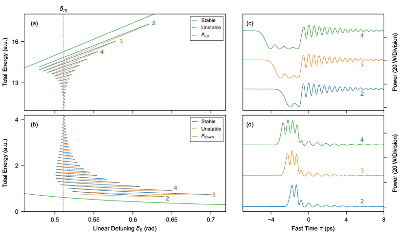
Figure S1: Numerically simulated collapsed snaking bifurcation structure. (a) and (b) show the bifurcation curves of dark and bright solitons under conditions of normal dispersion driving, respectively. Blue solid (dashed orange) curves correspond to stable (unstable) localized structures, whilst the green solid curves correspond to the upper and lower cw solutions of the system. (c) and (d) show examples of temporal profiles corresponding to dark and bright solitons, respectively. The simulation parameters are similar (albeit not identical) to the values used in our experiments: $L=26~{}\mathrm{m}$, $\mathcal{F}=45$, $\theta=0.05$, $\beta_{2}=0.5~{}\mathrm{ps^{2}/km}$, $\beta_{3}=0.2~{}\mathrm{ps^{3}/km}$, $\gamma=1.5~{}\mathrm{W^{-1}km^{-1}}$, $\theta=0.05$, $P_{\mathrm{in}}=2.9~{}\mathrm{W}$. The calculations ignore fourth-order dispersion and stimulated Raman scattering.

In Figs. S1(a) and (b), we show a typical collapsed snaking bifurcation structure, obtained by finding the localized steady-state solutions of Eq. (S1) under conditions of normal dispersion driving (see figure caption for parameters) using a Newton-Raphson continuation algorithm. Here we plot the integrated energy of the intracavity field as a function of the cavity detuning, with solid blue (dashed orange) curves corresponding to stable (unstable) solutions. Also shown as green solid curves are the energy levels corresponding to the homogeneous continuous wave (cw) steady-state solutions of the system, which map out an $S$-shaped profile characteristic of bistability.

As can be seen in Figs. S1(a) and (b), the bifurcation curve is composed of layers that fold on top of each other and that overlap over a finite range of detunings. Each layer corresponds to a localized structure characterized by a certain number of dips [for dark solitons (a)] or peaks [for bright solitons, (b)] in its temporal profile; Figs. S1(c) and (d) highlight that, moving vertically from one layer to another causes the number of peaks (or dips) to change by one. It is worth noting that, for parameters used in Fig. S1, the single-peak bright soliton does not exist (see also section “Bifurcation curve corresponding to experimental parameters” below).

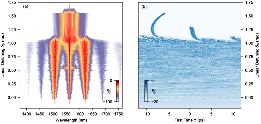
Figure S2: Numerically simulated results, showing the spontaneous excitation of bright localized structures via fourth-order modulation instability. Pseudo-color plots in (a) and (b) respectively show the spectral and temporal evolution of the intracavity field as the detuning is slowly increased. The temporal profiles are plotted in a reference frame that is close to the group velocity of the bright structures. Simulation parameters: $L=26~{}\mathrm{m}$, $\mathcal{F}=45$, $\theta=0.05$, $\beta_{2}=0.133~{}\mathrm{ps^{2}/km}$, $\beta_{3}=0.133~{}\mathrm{ps^{3}/km}$, $\beta_{4}=-9\times 10^{-4}~{}\mathrm{ps^{4}/km}$, $\gamma=1.5~{}\mathrm{W^{-1}km^{-1}}$, $\theta=0.05$, $P_{\mathrm{in}}=6.7~{}\mathrm{W}$. The calculations ignore stimulated Raman scattering.

A salient characteristic of the collapsed snaking bifurcation curve is that the range of existence of bright (dark) solitons tends to reduce as the number of peaks (dips) in its temporal profile increases. For very large number of peaks (or dips), the structures only exist over a narrow range around a particular detuning $\delta_{\mathrm{M}}$. This corresponds to the so-called Maxwell point: a unique point where fronts are motionless even without interacting, thus theoretically allowing dark or bright structures with arbitrary width.

I Impact of fourth-order dispersion

As mentioned in our main manuscript, the primary impact of fourth-order dispersion is that it renders the upper-state of the bistable cw cavity response unstable against modulation instability (MI). Ignoring SRS, the phase-matching condition for the four-wave mixing process that underpins MI can be written as sayson_octave-spanning_2019

$$\frac{\beta_{4}\Omega^{4}L}{24}+\frac{\beta_{2}\Omega^{2}L}{2}+2\gamma PL-\delta_{0}=0,$$ (S2)

where $\Omega=\omega-\omega_{\mathrm{p}}$ describes an (angular) frequency shift of a sideband at $\omega$ from the pump at $\omega_{\mathrm{p}}$, $P$ is the power level of the cw steady-state solution of Eq. (S1), and $\beta_{2}$ and $\beta_{4}$ are the second- and fourth-order dispersion coefficients at the pump frequency, respectively. It should be evident that a negative fourth-order dispersion coefficient can compensate for positive second-order dispersion at large frequency-shifts, thus enabling phase-matching and MI under conditions of normal dispersion driving.

Our experimental system exhibits a negative fourth-order dispersion coefficient, and so the upper cw state exhibits MI. As a consequence, it is not possible to sustain dark solitons in our system. (Since the cw state that surrounds them is unstable.) With regards to bright solitons, the main impact of fourth-order dispersion is to offer a convenient route to excite the solitons simply by scanning the laser frequency (detuning) across a cavity resonance. This is illustrated in Fig. S2, where we show an example of numerically simulated dynamics as the detuning is adiabatically scanned over a resonance, obtained by integrating Eq. (S1) with the split-step Fourier method [see figure caption for parameters]. As can be seen, the intracavity field initially corresponds to a cw state, but then undergoes MI at a detuning of about $\delta_{0}\approx-0.1~{}\mathrm{rad}$. As the detuning increases further beyond $\delta_{0}\approx 1.15~{}\mathrm{rad}$, we see the spontaneous emergence of bright localized structures characterized by different numbers of peaks that cease to exist at different detunings.

Figure S3: Theoretically predicted soliton spectrum in the presence ($\beta_{4}=-9\times 10^{-4}~{}\mathrm{ps^{2}/km}$, orange curve) and absence ($\beta_{4}=0$, blue curve) of fourth-order dispersion. The linear cavity detuning $\delta_{0}=0.7~{}\mathrm{rad}$ with all other parameters as in Fig. S2

We must emphasize that, other than facilitating their excitation, fourth-order dispersion does not significantly affect the characteristics of the bright solitons. This is illustrated in Fig. S3, where we plot spectra corresponding to steady-state soliton solutions of Eq. (S1) both in the presence and absence of fourth-order dispersion [other parameters as in Fig. S2]. Two important conclusions can be drawn: (i) the soliton indeed exists even without fourth-order dispersion, and (ii) fourth-order dispersion does not materially impact on the soliton characteristics. In this context, the fact that the soliton solutions exist even in the complete absence of fourth-order dispersion should make clear that the solitons do not correspond to localized elements of any $\beta_{4}$-induced MI pattern. This fact is also evidenced by the disparity between spectra in the MI and soliton regimes seen in Fig. S2(a). It appears that, whilst $\beta_{4}$ can facilitate the excitation of the normal-dispersion solitons, the origins of the two phenomena are dynamically distinct, one related to third-order dispersion (solitons) and the other related to fourth-order dispersion (MI).

II Bifurcation curve corresponding to experimental parameters

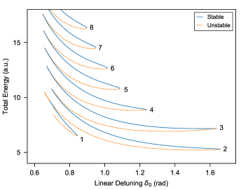
Figure S4: Theoretically predicted bifurcation curve of bright solitons corresponding to our experimental parameters. Numbers correspond to the number of peaks in the solitons’ temporal profile. The curves are somewhat different to those shown in Fig. 3 of our main manuscript as the total energy here includes the cw pump component.

For completeness, Fig. S4 shows the numerically computed bifurcation curve of bright solitons for our experimental parameters. (The curve is obtained from Eq. (S1) with both higher-order dispersion and stimulated Raman scattering included.) Theoretical results shown in Figs. 2–4 of our main manuscript are representative of this bifurcation curve.

It is worth noting that the bifurcation curve shown in Fig. S4 includes the single-peak soliton that is reminiscent of conventional cavity solitons in the anomalous dispersion regime. This should be contrasted with the illustrative results shown in Fig. S1: the parameters used in that case are such that single-peak solitons do not exist. Taken together, these results illustrate that (i) multi-peak bright structures can exist even for parameters for which single-peak solitons do not exist, and (ii) when single-peak solitons do exist, they are part of the same bifurcation curve as the multi-peak structures.

III measurement of resonator dispersion

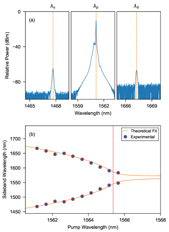
Figure S5: (a) Example of an MI spectrum recorded with driving wavelength $\lambda_{\mathrm{P}}=1561$ nm. The entire spectrum is divided into three panels for clarity: one for each sideband (left and right) and one for the pump (middle). (b) Solid dots show experimentally measured sideband wavelengths for a range of pump wavelengths. Solid curves show theoretical fit as explained in the text. The location of the zero-dispersion wavelength is indicated by the dashed red line.

To measure the dispersion of the resonator used in our experiments, we record the MI sidebands at various pump wavelengths, and fit Eq. (S2) to the experimentally observed tuning curve. To facilitate the analysis of the results, the cavity detuning is stabilized at zero, and the input power is kept as low as possible (whilst still observing MI). Thanks to these procedures, the two last terms in Eq. (S2) can be ignored.

Figure S5(a) shows an illustrative spectrum measured for a pump wavelength of $\lambda_{\mathrm{P}}=1561$ nm, which lies in the normal dispersion regime. We observe widely detuned sidebands at $\lambda_{\mathrm{u}}=1467.68$ and $\lambda_{\mathrm{d}}=1667.26$ nm. By measuring such spectra for a range of pump wavelengths, we obtain the tuning graph shown by the solid circles in Fig. S5(b). We then extract the dispersion characteristics of the resonator by fitting Eq. (S2) into the measured data. More specifically, there are three fitting parameters: the zero-dispersion wavelength $\lambda_{\mathrm{ZDW}}$ and the third- and fourth-order dispersion coefficients $\beta_{3,\mathrm{ZDW}}$ and $\beta_{4,\mathrm{ZDW}}$ at the ZDW, respectively. These parameters define the dispersion coefficients $\beta_{2}$ and $\beta_{4}$ appearing in Eq. (S2) at different pump wavelengths $\lambda_{\mathrm{P}}$ viz.

$$\beta_{2} =\beta_{3,\text{ZDW}}\Omega+\frac{\beta_{4,\text{ZDW}}}{2}\Omega^{2},$$

$$\beta_{4} =\beta_{4,\text{ZDW}},$$

where $\Omega=2\pi c\left[\lambda_{\mathrm{P}}^{-1}-\lambda_{\mathrm{ZDW}}^{-1}\right]$ with $c$ the speed of light in vacuum.

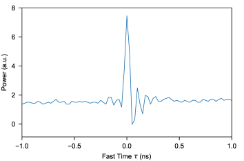
Figure S6: Typical photodetector trace measured at the 1% output port of our cavity, providing direct evidence of a bright localized structure.

One caveat with the method described above is that, due to the presence of three unknowns, an accurate fit to the equation using sideband data alone is relatively difficult, especially if the driving wavelength range is limited. In particular, we find that multiple combinations of parameters can yield reasonably good agreement with the experimental data. In order to reduce ambiguity, in addition to fitting Eq. S2, we also compare the experimentally measured spectra of normal-dispersion solitons with the spectra predicted by the theory for the dispersion coefficients that provide a reasonable fit to the phase matching curve. This two-step procedure yields the following parameters: $\lambda_{\mathrm{ZDW}}=1565.37$ nm, $\beta_{2,\mathrm{ZDW}}=0~{}\mathrm{ps}^{2}/\mathrm{km}$ (by definition), $\beta_{3,\mathrm{ZDW}}=0.135~{}\mathrm{ps}^{2}/\mathrm{km}$ and $\beta_{4,\mathrm{ZDW}}=-9\times 10^{-4}~{}\mathrm{ps}^{4}/\mathrm{km}$. The solid curves in Fig. S5 show the corresponding fit, and we see very good agreement. We believe these dispersion parameters obtained are very accurate, as they are capable of producing theoretical predictions of normal-dispersion solitons that agree with our experimental observations across a range of wavelengths, pump powers, linear detuning, and soliton types (as demonstrated in the main text).

IV Evidence of bright structures

All of the localized structures studied in our work correspond to bright structures, i.e., pulses of light that sit atop a low-intensity background. This fact can be observed directly from the photodetector signals measured at the 1% output port of our cavity. Figure S6 shows a typical example of such a photodetector signal, and indeed, we see a pulse that sits atop a background. We must emphasize that the 80 ps response time of our detection system is far too slow to resolve the soliton’s temporal profile, yet nevertheless, the signal shown in Fig. S6 provides unequivocal evidence of the structure’s bright (rather than dark) character.

References

- (1) M. Haelterman, S. Trillo, and S. Wabnitz, “Dissipative modulation instability in a nonlinear dispersive ring cavity,” Opt. Commun. 91, 401 (1992).
- (2) S. Coen, H. G. Randle, T. Sylvestre, and M. Erkintalo, “Modeling of octave-spanning Kerr frequency combs using a generalized mean-field Lugiato–Lefever model,” Opt. Lett. 38, 37 (2013).
- (3) C. Milián, A. V. Gorbach, M. Taki, A. V. Yulin, and D. V. Skryabin, “Solitons and frequency combs in silica microring resonators: Interplay of the Raman and higher-order dispersion effects,” Phys. Rev. A 92, 033851 (2015).
- (4) Y. Wang, M. Anderson, S. Coen, S. G. Murdoch, and M. Erkintalo, “Stimulated Raman Scattering Imposes Fundamental Limits to the Duration and Bandwidth of Temporal Cavity Solitons,” Phys. Rev. Lett. 120, 053902 (2018).
- (5) I. Hendry, B. Garbin, S. G. Murdoch, S. Coen, and M. Erkintalo, “Impact of de-synchronization and drift on soliton-based Kerr frequency combs in the presence of pulsed driving fields,” Phys. Rev. A 100, 023829 (2019).
- (6) R. H. Stolen, J. P. Gordon, W. J. Tomlinson, and H. A. Haus, “Raman response function of silica-core fibers,” J. Opt. Soc. Am. B 6, 1159–1166 (1989).
- (7) D. Hollenbeck and C. D. Cantrell, “Multiple-vibrational-mode model for fiber-optic Raman gain spectrum and response function,” J. Opt. Soc. Am. B 19, 2886–2892 (2002).
- (8) P. Parra-Rivas, D. Gomila, and L. Gelens, “Coexistence of stable dark- and bright-soliton Kerr combs in normal-dispersion resonators,” Phys. Rev. A 95, 053863 (2017).
- (9) N. L. B. Sayson, T. Bi, V. Ng, H. Pham, L. S. Trainor, H. G. L. Schwefel, S. Coen, M. Erkintalo, and S. G. Murdoch, “Octave-spanning tunable parametric oscillation in crystalline Kerr microresonators,” Nat. Photonics 13, 701–706 (2019).