The More the Merrier?! Evaluating the Effect of Landmark Extraction Algorithms on Landmark-Based Goal Recognition

Abstract

Recent approaches to goal and plan recognition using classical planning domains have achieved state of the art results in terms of both recognition time and accuracy by using heuristics based on planning landmarks. To achieve such fast recognition time these approaches use efficient, but incomplete, algorithms to extract only a subset of landmarks for planning domains and problems, at the cost of some accuracy. In this paper, we investigate the impact and effect of using various landmark extraction algorithms capable of extracting a larger proportion of the landmarks for each given planning problem, up to exhaustive landmark extraction. We perform an extensive empirical evaluation of various landmark-based heuristics when using different percentages of the full set of landmarks. Results show that having more landmarks does not necessarily mean achieving higher accuracy and lower spread, as the additional extracted landmarks may not necessarily increase be helpful towards the goal recognition task.

1 Introduction

Anticipating and recognizing correctly the intended goal that an observed agent aims to achieve based on its interactions in an environment is an important task for several real-world applications (?), such as intent recognition for elder-care (?), exploratory domain models (?; ?), offline and online goal recognition in latent space (?; ?; ?), and others. Most approaches to goal and plan recognition rely on either plan libraries (?; ?; ?; ?) or planning domain theory (?; ?; ?; ?; ?; ?). Recent work on goal recognition as planning has avoided running a full-fledged planner for recognizing goals, and recent approaches in the literature have successfully exploited the use of well-known automated planning techniques, such as planning graphs (?) and landmarks (?; ?; ?). Thus, as a result of exploiting planning techniques, such approaches have shown that it is possible to recognize goals and plans not only accurately, but also very quickly.

In this paper, we investigate the effect of using various landmark extraction algorithms over the landmark-based heuristic to goal recognition proposed by Pereira, Oren, and Meneguzzi (?). For extracting landmarks, we use five landmark extraction algorithms (?; ?; ?; ?) from the planning literature. To do so, we use an exhaustive extraction algorithm (i.e., an extraction approach that exhaustively checks if all facts are landmark by using a relaxed planning graph), and use other extraction algorithms that extract only a subset of landmarks (?; ?; ?; ?). Thus, the main contribution of this paper is investigating the real impact of using more or fewer landmarks in the landmark-based goal recognition heuristics.

We conduct extensive experiments to empirically evaluate the impact and effect of using a variety different landmark extraction algorithms over landmark-based recognition heuristics using well-known recognition datasets (?) with missing and full observations, and noisy, missing, and full observations. Results show that using more landmarks does not necessarily lead to improved precision and accuracy of the landmark-based heuristics, as the quality of the extracted landmarks is generally more important than the quantity.

The remainder of this paper is organized as follows. Section 2 provides essential background on planning, goal recognition, and landmarks. We review the landmark-based heuristic approaches we use along with various landmark extraction algorithms in Section 3. In Section 4, we proceed to evaluate empirically the recognition heuristics we review. Finally, in Section 5, we conclude this paper by discussing the real impact of using more or fewer landmarks in the heuristics, and provide future directions of how such heuristics could be improved by taking advantage of more landmarks.

2 Background

2.1 Planning

Planning is the problem of finding a sequence of actions (i.e., a plan) that achieves a goal from an initial state (?). A state is a finite set of facts that represent logical values according to some interpretation. Facts can be either positive, or negated ground predicates. A predicate is denoted by an n-ary predicate symbol $p$ applied to a sequence of zero or more terms ($\tau_{1}$, $\tau_{2}$, …, $\tau_{n}$). An operator is represented by a triple $a$ $=$ $\langle$name($a$), pre($a$), eff($a$)$\rangle$ where name($a$) represents the description or signature of $a$; pre($a$) describes the preconditions of $a$ — a set of facts or predicates that must exist in the current state for $a$ to be executed; $\mathit{eff}($a$)=\mathit{eff}(a)^{+}\cup\mathit{eff}(a)^{-}$ represents the effects of $a$, with eff($a$)⁺ an add-list of positive facts or predicates, and eff($a$)^- a delete-list of negative facts or predicates. When we instantiate an operator over its free variables, we call the resulting ground operator an action. A planning instance is represented by a triple $\Pi=\langle\Xi,\mathcal{I},G\rangle$, in which $\Xi=\langle\Sigma,\mathcal{A}\rangle$ is a planning domain definition; $\Sigma$ consists of a finite set of facts and $\mathcal{A}$ a finite set of actions; $\mathcal{I}$ $\subseteq$ $\Sigma$ is the initial state; and $G$ $\subseteq$ $\Sigma$ is the goal state. A plan is a sequence of actions $\pi=\langle a_{1},a_{2},...,a_{n}\rangle$ that modifies the initial state $\mathcal{I}$ into one in which the goal state $G$ holds by the successive execution of actions in a plan $\pi$. While actions have an associated cost, as in classical planning, in this paper we assume that this cost is 1 for all actions. A plan $\pi$ is considered optimal if its cost, and thus length, is minimal.

2.2 Goal Recognition

Goal recognition is the task of discerning the intended goal of autonomous agents or humans by observing their interactions in a particular environment (?, Chapter 1). Such observed interactions are defined as available evidence that can be used to recognize goals. We formally define the problem of goal recognition over planning domain theory by adopting the formalism proposed by Ramírez and Geffner (?; ?), as follows in Definition 1.

Definition 1 (Goal Recognition Problem).

A goal recognition problem is a tuple $T_{GR}$ $=$ $\langle\Xi,\mathcal{I},\mathcal{G},O\rangle$, in which $\Xi=\langle\Sigma,\mathcal{A}\rangle$ is a planning domain definition; $\mathcal{I}$ is the initial state; $\mathcal{G}$ is the set of possible goals, which include the correct intended goal $G^{*}$ (i.e., $G^{*}$ $\in$ $\mathcal{G}$); and $O$ $=$ $\langle$$o_{1}$, $o_{2}$, …, $o_{n}$$\rangle$ is an observation sequence of executed actions, with each observation $o_{i}\in\mathcal{A}$.

The ideal solution for a goal recognition problem is finding the correct intended goal $G^{*}\in\mathcal{G}$ that the observation sequence $O$ of a plan execution achieves. An observation sequence can be full or partial — in a full observation sequence we observe all actions of an agent’s plan; in a partial observation sequence, only a sub-sequence of actions are observed. A noisy observation sequence contains one or more actions (or a set of facts) that might not be part of a plan that achieves a particular goal, e.g., when a sensor fails and generates abnormal or spurious readings.

2.3 Landmarks

In the planning literature, landmarks are defined as necessary fact (or actions) that must be true (or executed) at some point along all valid plans that achieve a particular goal from an initial state. Landmarks are often partially ordered based on the sequence in which they must be achieved. Hoffman et al. (?) define fact landmarks as follows:

Definition 2 (Fact Landmark).

Given a planning instance $\Pi=\langle\Xi,\mathcal{I},G\rangle$, a formula $L$ is a fact landmark in $\Pi$ iff $L$ is true at some point along all valid plans that achieve $G$ from $\mathcal{I}$. A landmark is a type of formula (e.g., a conjunctive or disjunctive formula) over a set of facts that must be satisfied at some point along all valid plan executions.

Hoffman et al. (?) proves that the process of generating all landmarks and deciding their ordering is PSPACE-complete, which is exactly the same complexity as deciding plan existence (?). Thus, to operate efficiently, most landmark extraction algorithms extract only a subset of landmarks for a given planning instance.

2.4 Landmark Extraction Algorithms

In this paper, we use the following landmark extraction algorithms to investigate how the number of landmarks impacts on the recognition accuracy of landmark-based heuristics for goal recognition.

Exhaust: The first algorithm is an exhaustive extraction approach, its name says for itself, and we denote this algorithm as Exhaust. This algorithm exhaustively extracts landmarks for a given planning instance. Namely, this algorithm uses a Relaxed Planning Graph (RPG) and exhaustively checks every fact in the RPG for if it is a landmark or not. This is done by removing the fact from the RPG and checking if the goal is still reachable without the given fact, and if not, such fact is considered as a landmark. The number of landmarks extracted by this algorithm is used as a baseline in our experiments, as it can extract all landmarks for a planning instance.

$h^{m}$: ? (?) developed a landmark extraction algorithm that performs a transformation of the original problem $\Pi$, originating a new problem $\Pi^{m}$, in which each fact is a set of facts of size $m$, originated from the original problem’s facts. The actions are obtained by adding facts that are not required or caused by any action but might be true during plan development, to the action’s preconditions and effects. The result is a problem without delete effects that yet has information on the delete effects of the original problem, hence allowing the extraction of landmarks that take delete effects into count. This extraction algorithm is denoted as $h^{m}$.

RHW: In (?), ? (?) develop a landmark extraction algorithm that starts the process by selecting an initial fact landmark, and from this initial landmark, it creates disjunctive sets from the preconditions of the actions that are first achievers of the initial landmark. Each disjunctive set is then recorded as a landmark, and ordered before the initial landmark. This extraction process is then repeated for all recorded landmarks. We denote this algorithm as RHW.

Zhu & Givan: Zhu and Givan (?) developed a landmark extraction algorithm that works differently than the ones mentioned above. This algorithm works by propagating labels across the planning graph, where each label is a fact or an action. A fact or action at a level $i$ must be labeled with any fact or action that must occur in any $i$-step plan that reaches it. It starts by labeling each action in the first action level with itself. Every subsequent action level is then labeled with the union of the labels on its precondition fact nodes, while every subsequent fact node is labeled with the intersection of the labels on the action nodes that reach it. At the last level, every label on a goal node is considered a landmark. This algorithm is denoted as Zhu & Givan.

Hoffmann et al.: The extraction algorithm originally used by (?) is the landmark extraction algorithm of Hoffman et al. (?). Initially, this algorithm builds an RPG (ignoring all delete effects of all actions) from the initial state to the goal state, and starts selecting all facts in goal state as candidate landmarks. Afterward, it selects the preconditions for all actions that achieve each candidate landmark, checking if those are landmarks by removing them from the graph and checking the reachability of the goal. After, it records as landmarks all preconditions that passed this check and then repeats the process for every fact level on the graph back to the initial state. Similar to the Exhaust method, this algorithm evaluates whether a candidate landmark is indeed a landmark by testing the solvability of the problem by removing all actions that achieve such candidate landmark, and if the problem is unsolvable, then this candidate landmark is indeed a landmark. We denote this algorithm as Hoffmann et al.

3 Landmark-Based Goal Recognition

We now describe the goal recognition heuristics that rely on planning landmarks that we use to evaluate the effect of using different landmark extraction algorithms. Such heuristics have proved to be accurate and very quick for recognizing goals over a variety of domain models (?; ?).

The first landmark-based heuristic proposed by Pereira, Oren, and Meneguzzi (?) is called goal completion heuristic, and denoted as $\mathit{h}_{gc}$. Basically, this heuristic computes a score for a goal $G$ by calculating the ratio between the number achieved landmarks for $G$ and the total number of extracted landmarks for $G$. This score represents the percentage of completion of goal based on the ratio of achieved landmarks and the total number of landmarks.

As an extension of $\mathit{h}_{gc}$, the second heuristic developed by Pereira, Oren, and Meneguzzi (?) exploits the concept of landmark uniqueness value (?), which is a value that represents how unique a landmark is among the set of landmarks for all possible goals. This heuristic is called landmark uniqueness heuristic, and denoted as $\mathit{h}_{uniq}$. Thus, by using this uniqueness value, $\mathit{h}_{uniq}$ estimates which possible goal is most likely the intended one by summing the uniqueness values of the landmarks achieved in the observations.

4 Experiments and Evaluation

In this section, we present the experiments and evaluations we carried out from using various extraction algorithms over the landmark-based goal recognition heuristics.

4.1 Domains and Setup

For evaluating each one of the landmark extraction algorithms using both recognition heuristics, we executed several tests using datasets created by Pereira and Meneguzzi (?), containing several non-trivial recognition problems. These datasets contain goal recognition problems from 15 classical planning domains and include problems with noisy observations. The domains we used are: Blocks World, Campus, Depots, Dock Worker Robots, Driverlog, Easy IPC Grid, Ferry, Intrusion Detection, Logistics, Miconic, Rovers, Satellite, Sokoban and Zeno Travel. The Kitchen domain has been removed from our evaluation, as it is an adaptation of an HTN planning domain and it caused some issues when using some of the landmark extractors.

Each domain in these datasets includes recognition problems with partial and full observations. Partial observations vary the level (percentage) of observability between 10%, 30%, 50% and 70% of actions observed for missing observations, and 100% for full observations. For problems with noisy observations, the level (percentage) of observability varies between 25%, 50% and 75% of observed actions for missing observations, and consequently 100% for full observations.

4.2 Evaluation Metrics

To evaluate the recognition heuristics, we use three metrics: recognition time (Time), accuracy (Acc%) and Spread in $\mathcal{G}$ (S in $\mathcal{G}$). The recognition time metric is simply the time in seconds that the algorithm took to return the set of recognized goals, including the time for extracting the landmarks. Accuracy is a percentage that represents the average number of problems in which the correct goal was among the recognized goals list. Finally, Spread in $\mathcal{G}$ is the average number of returned goals, when multiple goal hypotheses were tied in the recognition algorithm. To have a concise precision metric of the approach, we combine accuracy and Spread in $\mathcal{G}$ to obtain a third metric. This metric can be considered as a precision metric and is obtained by calculating the ratio between accuracy and Spread in $\mathcal{G}$.

Since our goal is to find out if there is a relation between the number of extracted landmarks and the effectiveness of a landmark-based goal recognition technique, we also use a metric to evaluate the extraction capability of each landmark extraction algorithm. We do this by calculating the ratio between the number of landmarks extracted by each algorithm and the number of landmarks extracted by the Exhaust algorithm, since it can extract all landmarks in the planning instance. The result is the percentage of extracted landmarks.

4.3 Results: Missing and Full Observations

We now present the results for datasets with missing and full observations. Table 1 shows the results comparing the use of the five different extraction algorithms along with the landmark-based heuristics. We can see the average number of landmarks extracted, represented by $\mathcal{L}$, average recognition time in seconds, average accuracy (Acc%) and average Spread in $\mathcal{G}$ (S in $\mathcal{G}$) for each combination of extraction algorithm and threshold used for heuristics $h_{gc}$ and $h_{uniq}$. Columns represent different levels of observability.

		10%			30%			50%			70%			100%
Approach	$|\mathcal{L}|$	Time	Acc %	S in $\mathcal{G}$	Time	Acc %	S in $\mathcal{G}$	Time	Acc %	S in $\mathcal{G}$	Time	Acc %	S in $\mathcal{G}$	Time	Acc %	S in $\mathcal{G}$
$\mathit{h_{gc}}$ (Exhaust $\theta=0$)	36.9	5.848	63.4%	1.598	5.565	84.2%	1.259	6.708	89.9%	1.114	6.403	96.4%	1.048	6.874	99.6%	1.025
$\mathit{h_{gc}}$ (Exhaust $\theta=10$)	36.9	5.855	88.7%	3.378	5.558	96.9%	2.740	6.724	98.9%	2.421	6.377	99.6%	2.170	6.894	100.0%	1.869
$\mathit{h_{gc}}$ ($h^{m}$ $\theta=0$)	20.6	19.575	66.7%	1.634	19.844	83.2%	1.249	23.836	89.7%	1.143	21.725	96.5%	1.054	24.013	99.7%	1.046
$\mathit{h_{gc}}$ ($h^{m}$ $\theta=10$)	20.6	19.540	83.6%	2.819	19.860	92.8%	2.177	23.774	97.1%	1.930	21.677	99.2%	1.736	24.220	100.0%	1.474
$\mathit{h_{gc}}$ (RHW $\theta=0$)	23.5	5.793	64.8%	1.637	5.521	81.6%	1.251	6.664	89.1%	1.137	6.342	96.3%	1.062	6.872	99.5%	1.051
$\mathit{h_{gc}}$ (RHW $\theta=10$)	23.5	5.785	80.0%	2.735	5.536	91.2%	2.215	6.650	96.3%	2.000	6.328	98.6%	1.787	6.870	100.0%	1.509
$\mathit{h_{gc}}$ (Zhu & Givan $\theta=0$)	19.9	5.798	66.4%	1.657	5.523	83.1%	1.262	6.683	89.7%	1.147	6.338	96.4%	1.060	6.871	99.7%	1.054
$\mathit{h_{gc}}$ (Zhu & Givan $\theta=10$)	19.9	5.812	81.9%	2.768	5.534	92.6%	2.213	6.679	96.5%	1.947	6.331	98.6%	1.747	6.886	100.0%	1.483
$\mathit{h_{gc}}$ (Hoffmann $\theta=0$)	18.8	11.283	61.3%	1.630	10.648	77.1%	1.268	13.259	86.1%	1.149	12.500	94.1%	1.072	13.691	99.5%	1.056
$\mathit{h_{gc}}$ (Hoffmann $\theta=10$)	18.8	11.259	77.8%	2.743	10.721	87.4%	2.141	13.280	92.5%	1.850	12.509	96.5%	1.679	13.702	100.0%	1.454
$\mathit{h_{uniq}}$ (Exhaust $\theta=0$)	36.9	6.094	56.7%	1.153	5.681	76.8%	1.070	6.366	84.7%	1.035	5.938	93.4%	1.022	6.874	99.2%	1.025
$\mathit{h_{uniq}}$ (Exhaust $\theta=10$)	36.9	6.086	71.3%	1.881	5.696	87.1%	1.537	6.358	91.0%	1.325	5.909	97.2%	1.244	6.895	100.0%	1.130
$\mathit{h_{uniq}}$ ($h^{m}$ $\theta=0$)	20.6	20.892	58.0%	1.218	19.494	76.0%	1.071	22.266	85.3%	1.040	20.448	94.2%	1.028	23.853	99.7%	1.046
$\mathit{h_{uniq}}$ ($h^{m}$ $\theta=10$)	20.6	20.880	69.7%	1.772	19.467	84.6%	1.429	22.237	90.9%	1.287	20.408	97.1%	1.203	24.033	100.0%	1.112
$\mathit{h_{uniq}}$ (RHW $\theta=0$)	23.5	6.033	56.4%	1.214	5.665	74.8%	1.067	6.313	85.1%	1.039	5.854	93.8%	1.029	6.802	99.5%	1.051
$\mathit{h_{uniq}}$ (RHW $\theta=10$)	23.5	6.025	69.3%	1.815	5.639	84.1%	1.453	6.301	90.4%	1.306	5.871	96.7%	1.216	6.774	100.0%	1.121
$\mathit{h_{uniq}}$ (Zhu & Givan $\theta=0$)	19.9	6.031	56.8%	1.212	5.668	75.7%	1.070	6.315	85.0%	1.042	5.891	93.9%	1.031	6.785	99.7%	1.054
$\mathit{h_{uniq}}$ (Zhu & Givan $\theta=10$)	19.9	6.028	69.3%	1.788	5.647	84.9%	1.441	6.284	90.7%	1.291	5.882	96.8%	1.201	6.836	100.0%	1.112
$\mathit{h_{uniq}}$ (Hoffmann $\theta=0$)	18.8	11.903	53.4%	1.308	11.076	70.8%	1.117	12.383	80.2%	1.039	11.460	90.8%	1.032	13.610	98.5%	1.043
$\mathit{h_{uniq}}$ (Hoffmann $\theta=10$)	18.8	11.915	65.3%	1.868	11.044	79.9%	1.486	12.379	86.9%	1.328	11.422	93.9%	1.236	13.715	99.2%	1.120

Table 1: Experiments and evaluations with missing and full observations.

We can see that even with 100% of actions being observed, the heuristic recognition algorithms do not yield 100% accuracy. There are some cases, for instance, in Driverlog and Logistics for $\mathit{h_{gc}}$, in which the real goal had more total landmarks than a wrong candidate goal, but only a few extra achieved landmarks than the wrong one. As a result, the heuristic chooses the wrong goal instead the correct one, especially with lower threshold values.

We can also see that the extraction $h^{m}$ algorithm has the highest recognition time in comparison to all algorithms. Hoffmann et al. has the second highest recognition time, while other algorithms come in third with similar recognition time.

Figure 1 shows the average percentage of extracted landmarks by each extraction algorithm we used in our experiments for Table 1. Note that, after Exhaust, RHW was the extraction algorithm that managed to extract the highest number of landmarks, on average, followed by $h^{m}$, Zhu & Givan, and finally Hoffman et al..

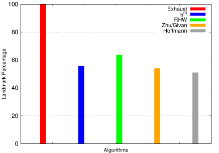
Figure 1: Percentage of extracted landmarks by algorithm with missing and full observations.

Figures 2 and 3 show the average Accuracy/Spread in $\mathcal{G}$ ratio with a threshold $\theta$ value of 10 for each combination of heuristic, extraction algorithm, and the level of observability. Although Exhaust and RHW managed to extract the highest number of landmarks, $h^{m}$ was the algorithm that led both heuristics to the highest Accuracy/Spread in $\mathcal{G}$ ratio, leaving even Exhaust behind.

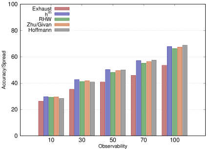
Figure 2: Accuracy/Spread in $\mathcal{G}$ ratio for $\mathit{h_{gc}}$ with missing and full observations.

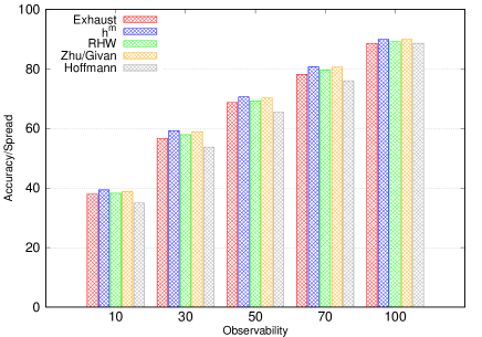
Figure 3: Accuracy/Spread in $\mathcal{G}$ ratio for $\mathit{h_{uniq}}$ with missing and full observations.

Based on the results of Figures 2 and 3, we can see that that the amount of extracted landmarks is not the only factor that affects the effectiveness for recognition using landmarks. We note that the quality of the extracted landmarks and how well they inform the heuristics cause real impact in the recognition process. We believe this is the reason $\mathit{h_{uniq}}$ yields a higher Accuracy/Spread ratio in the datasets with missing and full observations when compared to $\mathit{h_{gc}}$. The $\mathit{h_{uniq}}$ heuristic considers the degree of information provided by a landmark (i.e., landmark uniqueness values), instead of just estimating using the amount of landmarks, as $\mathit{h_{gc}}$ does. The $\mathit{h_{uniq}}$ heuristic can filter relatively uninformative landmarks, assigning a greater landmark uniqueness value for those that are found in fewer goals, hence better informing the heuristic.

Figures 4 and 5, show how the recognition time varies with the growth of observation length for $\mathit{h_{gc}}$ and $\mathit{h_{uniq}}$, respectively. We can see that all algorithms provide a close to constant recognition time, except for $h^{m}$, in which we see the recognition time grows as the observation grows in length. Note that some curves are overlaid by others, causing them to not appear.

Note that the sequence of observations does not have a direct impact on the landmark extraction algorithms since they are not provided to the algorithms. However, longer observations generally translate to more complex problems, resulting in the increasing recognition time.

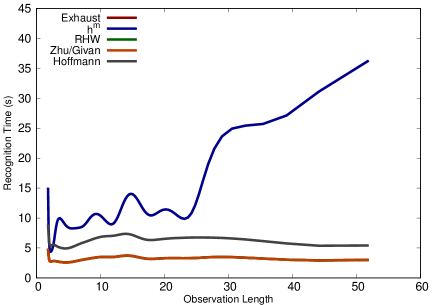
Figure 4: Recognition time for $\mathit{h_{gc}}$ with missing and full observations.

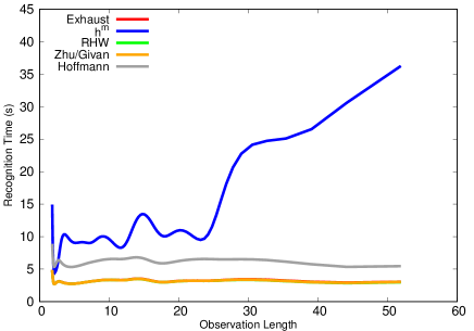
Figure 5: Recognition time for $\mathit{h_{uniq}}$ with missing and full observations.

4.4 Results: Noisy, Missing, and Full Observations

In this section, we present and analyze the results obtained by experimenting the different recognition approaches in problems under noisy observations. We refer to noisy observations as a set of observed actions in which some of the actions are spurious actions. As mentioned before, for the datasets with noisy observations, we have 4 levels of observability, as follows: 25%, 50%, 75%, and 100%.

We can see the results for both recognition heuristics in Table 2. This table has the same format as the one presented in the previous section, for missing and full observations, the only difference is the number of columns, as now we have four observability levels instead of five.

		25%			50%			75%			100%
Approach	$|\mathcal{L}|$	Time	Acc %	S in $\mathcal{G}$	Time	Acc %	S in $\mathcal{G}$	Time	Acc %	S in $\mathcal{G}$	Time	Acc %	S in $\mathcal{G}$
$\mathit{h_{gc}}$ (Exhaust $\theta=0$)	29.8	4.823	47.5%	1.421	5.787	73.5%	1.237	5.148	87.3%	1.111	5.924	95.7%	1.085
$\mathit{h_{gc}}$ (Exhaust $\theta=10$)	29.8	4.829	72.2%	3.149	5.759	90.7%	2.832	5.174	96.8%	2.356	5.947	99.7%	2.171
$\mathit{h_{gc}}$ ($h^{m}$ $\theta=0$)	17.5	10.702	49.5%	1.526	12.531	73.4%	1.272	11.316	86.9%	1.121	13.648	95.7%	1.125
$\mathit{h_{gc}}$ ($h^{m}$ $\theta=10$)	17.5	10.685	65.7%	2.693	12.483	85.6%	2.326	11.351	95.3%	1.944	13.680	98.7%	1.752
$\mathit{h_{gc}}$ (RHW $\theta=0$)	19.7	4.778	48.8%	1.504	5.726	72.9%	1.284	5.126	86.8%	1.140	5.895	95.1%	1.129
$\mathit{h_{gc}}$ (RHW $\theta=10$)	19.7	4.771	64.1%	2.535	5.707	84.4%	2.244	5.098	94.4%	1.926	5.909	98.3%	1.692
$\mathit{h_{gc}}$ (Zhu & Givan $\theta=0$)	16.8	4.814	48.3%	1.520	5.737	73.4%	1.280	5.116	86.9%	1.131	5.921	94.7%	1.131
$\mathit{h_{gc}}$ (Zhu & Givan $\theta=10$)	16.8	4.793	65.7%	2.655	5.726	84.8%	2.330	5.111	94.3%	1.966	5.931	98.1%	1.700
$\mathit{h_{gc}}$ (Hoffmann $\theta=0$)	16.3	9.267	44.9%	1.465	11.572	68.8%	1.282	10.069	82.4%	1.185	12.068	91.3%	1.153
$\mathit{h_{gc}}$ (Hoffmann $\theta=10$)	16.3	9.181	61.2%	2.462	11.602	81.2%	2.256	9.976	90.1%	1.965	12.047	95.9%	1.748
$\mathit{h_{uniq}}$ (Exhaust $\theta=0$)	29.8	4.280	38.5%	1.098	5.546	62.4%	1.069	4.510	82.1%	1.050	6.149	93.8%	1.050
$\mathit{h_{uniq}}$ (Exhaust $\theta=10$)	29.8	4.270	52.6%	1.768	5.501	75.6%	1.612	4.500	88.7%	1.369	6.210	96.7%	1.337
$\mathit{h_{uniq}}$ ($h^{m}$ $\theta=0$)	17.5	9.050	39.1%	1.164	11.096	62.7%	1.062	9.407	82.3%	1.054	12.711	94.2%	1.093
$\mathit{h_{uniq}}$ ($h^{m}$ $\theta=10$)	17.5	9.053	50.9%	1.734	11.095	74.1%	1.598	9.386	88.7%	1.354	12.836	97.0%	1.293
$\mathit{h_{uniq}}$ (RHW $\theta=0$)	19.7	4.254	38.7%	1.152	5.509	62.8%	1.064	4.501	81.3%	1.059	6.175	94.2%	1.095
$\mathit{h_{uniq}}$ (RHW $\theta=10$)	19.7	4.246	51.0%	1.747	5.495	75.1%	1.609	4.494	87.5%	1.354	6.169	96.5%	1.303
$\mathit{h_{uniq}}$ (Zhu & Givan $\theta=0$)	16.8	4.259	39.5%	1.172	5.484	62.7%	1.063	4.500	82.7%	1.062	6.191	94.2%	1.101
$\mathit{h_{uniq}}$ (Zhu & Givan $\theta=10$)	16.8	4.256	51.1%	1.756	5.503	74.7%	1.606	4.498	88.1%	1.364	6.200	96.7%	1.301
$\mathit{h_{uniq}}$ (Hoffmann $\theta=0$)	16.3	7.903	36.4%	1.138	11.022	59.7%	1.069	8.500	77.0%	1.065	12.859	88.3%	1.077
$\mathit{h_{uniq}}$ (Hoffmann $\theta=10$)	16.3	7.900	48.1%	1.742	11.104	70.7%	1.612	8.507	83.2%	1.419	12.951	92.7%	1.346

Table 2: Experiments and evaluations with missing, noisy and full observations.

We notice a drop in the accuracy metric by comparing the results in Tables 1 and 2 and argue that it is an expected behavior, as the noise within the observations tends to mislead the recognition heuristics into recognizing the wrong goals as correct. Also, as expected, the recognition time is unaffected with relation to noiseless observations, with $h^{m}$ having the longest recognition times, followed by Hoffmann et al. and the other algorithms. We can see that in noisy experiments, there is less difference between Hoffmann et al. and $h^{m}$ recognition times.

Figure 6 shows the average percentage of landmarks extracted by each algorithm for the datasets with noisy observations. This metric has to be recalculated for noisy observations, as the goal recognition problems with noisy observations are different from the ones without noise. We can see all algorithms, except for Exhaust, managed to achieve a higher percentage of achieved landmarks in comparison to noiseless experiments, as the number of landmarks extracted by Exhaust dropped. Yet, the algorithm ranking for the percentage of landmarks extracted remains similar to the noiseless experiments.

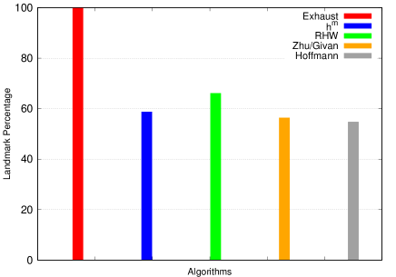
Figure 6: Percentage of extracted landmarks by algorithm with missing, noisy and full observations.

Figures 7 and 8 show the Accuracy/Spread in $\mathit{G}$ ratio for each algorithm and observability degree for a threshold value of 10, for $\mathit{h_{gc}}$ and $\mathit{h_{uniq}}$ respectively.

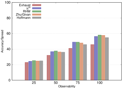
Figure 7: Accuracy/Spread in $\mathcal{G}$ ratio for $\mathit{h_{gc}}$ with missing, noisy and full observations.

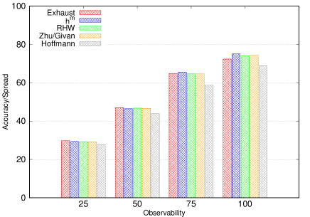
Figure 8: Accuracy/Spread in $\mathcal{G}$ ratio for $\mathit{h_{uniq}}$ with missing, noisy and full observations.

As for the results using the $\mathit{h_{gc}}$ heuristic, we can see a different scenario when comparing to noiseless experiments. With noisy observations, the extraction algorithm that had the best overall performance in Accuracy/Spread in $\mathcal{G}$ was RHW, which also extracted the most landmarks after Exhaust. RHW dominated the score for 25% and 50% observability levels, only being beaten by $h^{m}$ in 75% and Zhu & Givan in 100%.

With respect to the results of the $\mathit{h_{uniq}}$ heuristic results, we see the same behavior in noiseless experiments. Algorithms that extract a larger number of landmarks yielded better results in comparison to $\mathit{h_{gc}}$, as we can see from Exhaust results in 25% and 50% observability levels, only being beaten by $h^{m}$ in 75% and 100%.

From these results, we can see how the presence of noise in observations really affects the recognition with different landmark extraction algorithms. When we work with noisy observations, the number of landmarks extracted seems have a stronger impact. This can be explained by the fact that having irrelevant actions within the observations makes so that having more landmarks may help the heuristic while comparing them against the relevant observations, as noisy actions are unlikely to coincide within the landmarks for the correct goal.

Finally, in Figures 9 and 10, we can see the recognition time variation as observation length grows for $\mathit{h_{gc}}$ and $\mathit{h_{uniq}}$, respectively. A similar time marks can be seen without noisy observations, with $h^{m}$’s running time growing with observation length, while the other algorithms remain almost constant, with minor differences. We also see the same curve overlay effect that causes some curves to not appear.

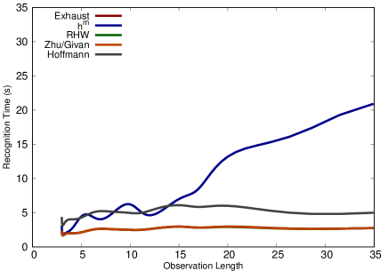
Figure 9: Recognition time for $\mathit{h_{gc}}$ with missing, noisy and full observations.

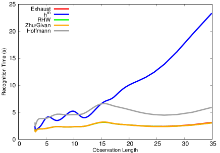
Figure 10: Recognition time for $\mathit{h_{uniq}}$ with missing, noisy and full observations.

5 Conclusions

We have presented an extensive empirical evaluation of how different landmark extraction algorithms affect the performance of landmark-based goal recognition approaches. After analyzing the results in the experiments, we conclude that the number of extracted landmarks does not tell us all about the quality or utility of a landmark when using it in landmark-based goal recognition. We can see from the results that having more landmarks is not necessarily more important than having informative landmarks.

As future work, we intend to perform a more qualitative analysis of the landmark extraction algorithms, analyzing not only the amount of extracted landmarks, but also the information level of the landmarks themselves. This ought to provide even more answers on what kind of extraction algorithm is best suited for landmark-based goal recognition, and consequently enabling us to fine-tune solutions to maximize the effectiveness of the goal recognition process. Finally, we aim to conduct a similar extensive empirical evaluation by using some of the landmark extraction algorithms over the landmark-based approaches under incomplete domain information (?; ?).

References

- [Amado et al. 2018a] Amado, L.; Aires, J. P.; Pereira, R. F.; Magnaguagno, M. C.; Granada, R.; and Meneguzzi, F. 2018a. Lstm-based goal recognition in latent space. CoRR abs/1808.05249.
- [Amado et al. 2018b] Amado, L.; Pereira, R. F.; Aires, J. P.; Magnaguagno, M.; Granada, R.; and Meneguzzi, F. 2018b. Goal recognition in latent space. In Proceedings of the 2018 International Joint Conference on Neural Networks (IJCNN).
- [Amado et al. 2019] Amado, L.; ao Paulo Aires, J.; Pereira, R. F.; Magnaguagno, M. C.; Granada, R.; Licks, G. P.; and Meneguzzi, F. 2019. LatRec: Recognizing Goals in Latent Space (Demo). In Proceedings of the 29th International Conference on Automated Planning and Scheduling (ICAPS).
- [Amir and Gal 2013] Amir, O., and Gal, Y. K. 2013. Plan Recognition and Visualization in Exploratory Learning Environments. ACM Transactions on Interactive Intelligent Systems 3(3):16:1–16:23.
- [Avrahami-Zilberbrand and Kaminka 2005] Avrahami-Zilberbrand, D., and Kaminka, G. A. 2005. Fast and Complete Symbolic Plan Recognition. In Proceedings of the International Joint Conference on Artificial Intelligence (IJCAI), 653–658.
- [Bylander 1994] Bylander, T. 1994. The Computational Complexity of Propositional STRIPS Planning. Journal of Artificial Intelligence Research (JAIR) 69:165–204.
- [E-Martín, R.-Moreno, and Smith 2015] E-Martín, Y.; R.-Moreno, M. D.; and Smith, D. E. 2015. A fast goal recognition technique based on interaction estimates. In Proceedings of the International Joint Conference on Artificial Intelligence (IJCAI), 761–768.
- [Geib and Goldman 2009] Geib, C. W., and Goldman, R. P. 2009. A Probabilistic Plan Recognition Algorithm Based on Plan Tree Grammars. Artificial Intelligence 173(11):1101–1132.
- [Geib 2002] Geib, C. W. 2002. Problems with Intent Recognition for Elder Care. In Proceedings of the Conference of the Association for the Advancement of Artificial Intelligence (AAAI), 13–17.
- [Ghallab, Nau, and Traverso 2004] Ghallab, M.; Nau, D. S.; and Traverso, P. 2004. Automated Planning - Theory and Practice. Elsevier.
- [Hoffmann, Porteous, and Sebastia 2004] Hoffmann, J.; Porteous, J.; and Sebastia, L. 2004. Ordered Landmarks in Planning. Journal of Artificial Intelligence Research (JAIR) 22(1):215–278.
- [Keren, Gal, and Karpas 2014] Keren, S.; Gal, A.; and Karpas, E. 2014. Goal Recognition Design. In Proceedings of the International Conference on Automated Planning and Scheduling (ICAPS).
- [Keyder, Richter, and Helmert 2010] Keyder, E.; Richter, S.; and Helmert, M. 2010. Sound and complete landmarks for and/or graphs. In ECAI.
- [Masters and Sardiña 2017] Masters, P., and Sardiña, S. 2017. Cost-Based Goal Recognition for Path-Planning. In Proceedings of the International Conference on Autonomous Agents and Multiagent Systems (AAMAS), 750–758.
- [Mirsky et al. 2017] Mirsky, R.; Stern, R.; Ya’akov (Kobi) Gal, M. K.; and Kalech, M. 2017. Plan Recognition Design. In Proceedings of the Conference of the Association for the Advancement of Artificial Intelligence (AAAI), 4971–4972.
- [Mirsky, Gal, and Shieber 2017] Mirsky, R.; Gal, Y. K.; and Shieber, S. M. 2017. CRADLE: An Online Plan Recognition Algorithm for Exploratory Domains. ACM Transactions on Intelligent Systems and Technology (TIST) 8(3):45:1–45:22.
- [Oh et al. 2013] Oh, J.; Meneguzzi, F.; Sycara, K.; and Norman, T. J. 2013. Prognostic normative reasoning. Engineering Applications of Artificial Intelligence 26(2):863 – 872.
- [Oh, Meneguzzi, and Sycara 2014] Oh, J.; Meneguzzi, F.; and Sycara, K. 2014. Probabilistic plan recognition for proactive assistant agents. In Sukthankar, G.; Goldman, R. P.; Geib, C.; Pynadath, D. V.; and Bui, H. H., eds., Plan, Activity, and Intent Recognition: Theory and Practice. Elsevier. 275–288.
- [Pattison and Long 2010] Pattison, D., and Long, D. 2010. Domain Independent Goal Recognition. In Starting AI Researcher Symposium (STAIRS).
- [Pereira and Meneguzzi 2016] Pereira, R. F., and Meneguzzi, F. 2016. Landmark-Based Plan Recognition. In Proceedings of the European Conference on Artificial Intelligence (ECAI).
- [Pereira and Meneguzzi 2017] Pereira, R. F., and Meneguzzi, F. 2017. Goal and Plan Recognition Datasets using Classical Planning Domains. At the data repository Zenodo.
- [Pereira and Meneguzzi 2018] Pereira, R. F., and Meneguzzi, F. 2018. Goal Recognition in Incomplete Domain Models. In Proceedings of the Conference of the Association for the Advancement of Artificial Intelligence (AAAI).
- [Pereira, Oren, and Meneguzzi 2017a] Pereira, R. F.; Oren, N.; and Meneguzzi, F. 2017a. Detecting Commitment Abandonment by Monitoring Sub-Optimal Steps During Plan Execution. In Proceedings of the 16th Conference on Autonomous Agents and MultiAgent Systems (AAMAS).
- [Pereira, Oren, and Meneguzzi 2017b] Pereira, R. F.; Oren, N.; and Meneguzzi, F. 2017b. Landmark-Based Heuristics for Goal Recognition. In Proceedings of the Conference of the Association for the Advancement of Artificial Intelligence (AAAI).
- [Pereira, Oren, and Meneguzzi 2017c] Pereira, R. F.; Oren, N.; and Meneguzzi, F. 2017c. Monitoring Plan Optimality using Landmarks and Domain-Independent Heuristics. In The AAAI 2017 Workshop on Plan, Activity, and Intent Recognition.
- [Pereira, Pereira, and Meneguzzi 2019] Pereira, R. F.; Pereira, A. G.; and Meneguzzi, F. 2019. Landmark-enhanced heuristics for goal recognition in incomplete domain models. In Proceedings of the Twenty-Ninth International Conference on Automated Planning and Scheduling ICAPS.
- [Ramírez and Geffner 2009] Ramírez, M., and Geffner, H. 2009. Plan Recognition as Planning. In Proceedings of the International Joint Conference on Artificial Intelligence (IJCAI).
- [Ramírez and Geffner 2010] Ramírez, M., and Geffner, H. 2010. Probabilistic Plan Recognition Using Off-the-Shelf Classical Planners. In Proceedings of the Conference of the Association for the Advancement of Artificial Intelligence (AAAI).
- [Silvia Richter 2008] Silvia Richter, M. H. e. M. W. 2008. Landmarks revisited. In Proceedings of the Twenty-Third AAAI Conference on Artificial Intelligence (2008).
- [Sohrabi, Riabov, and Udrea 2016] Sohrabi, S.; Riabov, A. V.; and Udrea, O. 2016. Plan Recognition as Planning Revisited. In Proceedings of the International Joint Conference on Artificial Intelligence (IJCAI).
- [Sukthankar et al. 2014] Sukthankar, G.; Goldman, R. P.; Geib, C.; Pynadath, D. V.; and Bui, H. H. 2014. Plan, Activity, and Intent Recognition: Theory and Practice. Elsevier.
- [Zhu and Givan 2003] Zhu, L., and Givan, R. 2003. Landmark extraction via planning graph propagation. In In ICAPS Doctoral Consortium.