Renormalization group theory of percolation on pseudo-fractal
simplicial and cell complexes

Abstract

Simplicial complexes are gaining increasing scientific attention as they are generalized network structures that can represent the many-body interactions existing in complex systems raging from the brain to high-order social networks. Simplicial complexes are formed by simplicies, such as nodes, links, triangles and so on. Cell complexes further extend these generalized network structures as they are formed by regular polytopes such as squares, pentagons etc. Pseudo-fractal simplicial and cell complexes are a major example of generalized network structures and they can be obtained by gluing $2$-dimensional $m$-polygons ($m=2$ triangles, $m=4$ squares, $m=5$ pentagons, etc.) along their links according to a simple iterative rule. Here we investigate the interplay between the topology of pseudo-fractal simplicial and cell complexes and their dynamics by characterizing the critical properties of link percolation defined on these structures. By using the renormalization group we show that the pseudo-fractal simplicial and cell complexes have a continuous percolation threshold at $p_{c}=0$. When the pseudo-fractal structure is formed by polygons of the same size $m$, the transition is characterized by an exponential suppression of the order parameter $P_{\infty}$ that depends on the number of sides $m$ of the polygons forming the pseudo-fractal cell complex, i.e., $P_{\infty}\propto p\exp(-\alpha/p^{m-2})$. Here these results are also generalized to random pseudo-fractal cell-complexes formed by polygons of different number of sides $m$.

I Introduction

Simplicial and cell complexes Bianconi (2015); Salnikov et al. (2018) are generalized network structures capturing the many-body interactions existing in complex systems such as brain networks Giusti et al. (2016); Petri et al. (2014); Reimann et al. (2017), social networks Petri and Barrat (2018); Iacopini et al. (2019); Alvarez-Rodriguez et al. (2020), and complex materials Papadopoulos et al. (2018); Šuvakov et al. (2018). Simplicial and cell complexes are not only formed by nodes and links like networks, but they are also formed by higher dimensional simplexes and polytopes such as triangles, squares, pentagons, etc. Being formed by geometrical and topological building blocks simplicial complexes are ideal structures to study network geometry Bianconi and Rahmede (2017a, b); Mulder and Bianconi (2018). Moreover, simplicial complexes are key to investigate the role that network geometry and many-body interactions have on dynamics. Among the vast variety of dynamical processes that are starting to be investigated on simplicial complexes we mention percolation Bianconi and Ziff (2018); Kryven et al. (2019); Bianconi et al. (2019); Hasegawa and Nemoto (2013), synchronization Skardal and Arenas (2019); Millán et al. (2020); Gambuzza et al. (2020); Lucas et al. (2020); Millán et al. (2018, 2019), epidemic spreading Iacopini et al. (2019); St-Onge et al. (2020), Gaussian models Bianconi and Dorogovstev (2020); Reitz and Bianconi (2020); Šuvakov et al. (2018), and random walks Torres and Bianconi (2020); Carletti et al. (2020). The vast majority of hierarchical networks studied in statistical mechanics and network theory literature is formed by the skeleton of simplicial and cell complexes (i.e., the network formed by its nodes and links). Examples range from the diamond network of Migdal and Kadanoff Migdal (1976); Kadanoff (1976) to the hyperbolic Farey graphs that have been shown to display a discontinuous percolation phase transition in Ref.  Boettcher et al. (2012). These networks are well suited to perform exact real-space renormalization group (RG) calculations. Using RG theory there has been very important progress in characterizing the critical properties of percolation Boettcher et al. (2012, 2009); Nogawa (2018); Hasegawa et al. (2010); Nogawa and Hasegawa (2014); Kryven et al. (2019); Bianconi and Ziff (2018); Bianconi et al. (2019); Auto et al. (2008), spin (Ising and Potts) models Boettcher and Brunson (2015); Singh et al. (2014); Boettcher and Brunson (2011); Hinczewski and Berker (2006), and Gaussian models Bianconi and Dorogovstev (2020); Reitz and Bianconi (2020) in these structures. In particular in Refs. Kryven et al. (2019); Bianconi et al. (2019) the robustness of the result obtained by Boettcher, Singh and Ziff in Ref.  Boettcher et al. (2012) has been investigated by considering more general simplicial and cell complexes. It has been found that two-dimensional simplicial and cell complexes, i.e., simplicial and cell complexes build by gluing two-dimensional polygons along their links, can display a large variety of critical behaviors for the order parameter of link percolation. Here we extend this line of research and we characterize the link percolation transition to random pseudo-fractal simplicial and cell complexes. Pseudo-fractal simplicial complexes have been originally proposed as deterministic model for complex networks in Ref.  Dorogovtsev et al. (2002). Link percolation on these deterministic pseudo-fractal networks has been discussed previously in Ref.  Dorogovtsev (2003). Here however we provide a more extensive treatment of the problem and are able to show that the critical percolation properties of the deterministic pseudo-fractal simplicial complex differs from the percolation properties of the deterministic pseudo-fractal cell complex and the random pseudo-fractal simplicial complexes. Indeed our work shows that for the deterministic pseudo-fractal simplicial complexes formed by $m$-polygons, the phase transition is at $p_{c}=0$ and the order parameter behaves as

$$P_{\infty}\propto p\exp(-\alpha/p^{m-2})$$ (1)

where $\alpha$ is a constant. Therefore the exponential suppression goes like $1/p$ for $m=3$ as obtained by Ref. Dorogovtsev (2003) but goes like $1/p^{m-2}$ for $m>3$. On a side note we mention also that our derivation also captures the factor $p$ in Eq. (1) not discussed in Ref.  Dorogovtsev et al. (2002). Finally for random pseudo-fractal simplicial complexes we show that the critical behavior is dictated by the smaller value of $m$ of the polygons of the cell complex.

The paper is structured as follows: in Sec.  II we describe the main properties of the random pseudo-fractal cell complexes studied in this work; in Sec.  III we introduce link percolation on pseudo-fractal cell complexes, we derive the iterative equations for the linking probability defining the RG equations, and we derive the expression for the generating functions and the for the order parameter in terms of the linking probability, in Sec.  IV we discuss the RG flow, in Sec. V we derive the critical behavior of the order parameter, finally in Sec.  VI we provide the conclusions.

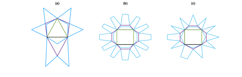
Figure 1: (Color online) Examples of pseudo-fractal simplicial and cell complexes represented at iteration $n=3$. Panel (a) shows a deterministic pseudo-fractal simplicial complex with $m=3$, panel (b) shows a deterministic pseudo-fractal cell complex with $m=4$, panel (c) shows a random pseudo-fractal cell complex with $q_{3}=q_{4}=1/2$. The different colors indicate the different iterations: $n=0$ (black), $n=1$ (green) $n=2$ (purple), $n=3$ (cyan).

II Random pseudo-fractal simplicial and cell complexes

The pseudo-fractal simplicial complex Dorogovtsev et al. (2002) is constructed iteratively starting at iteration $n=0$ from a single link. At each time $n\geq 1$ we attach a triangle to every link introduced at iteration $0\leq n^{\prime}<n$. This construction can be generalized by considering a random cell complex formed by regular $m$-polygons with different $m\geq 3$. We start at iteration $n=0$ from an initial link. At each iteration $n\geq 1$ we glue a $m$-polygon to every link of the cell complex introduced at iteration $0\leq n^{\prime}<n$ with $m\geq 3$ drawn from a $q_{m}$ distribution. Is is easy to show that at iteration $n$ the expected number of nodes $\overline{N}_{n}$ and links $\overline{L}_{n}$ are given by

$$\overline{N}_{n} = 2+\frac{\langle{m}\rangle-2}{\langle{m}\rangle-1}(\langle{m}\rangle^{n}-1),$$

$$\overline{L}_{n} = \langle{m}\rangle^{n},$$ (2)

where $\langle{m}\rangle=\sum_{m\geq 3}mq_{m}$. In the following we will refer to these generalized network structures as random cell complexes. However for $q_{m}=\delta_{m,3}$ the random pseudo-fractal cell complex reduces to the pseudo-fractal simplicial complex (see Fig.  1a). Moreover for $q_{m^{\prime}}=\delta_{m^{\prime},m}$ and $m>3$ we obtain a deterministic cell complex formed by gluing only $m$-polygons. (see Fig.  1b for an example of a deterministic cell complex with $m=4$). Only if the distribution $q_{m}$ is not a Kronecker delta, the model reduces to a genuine random cell complex (see Fig.  1b for an example of a random cell complex with $q_{3}=q_{4}=1/2$).

III Link percolation on pseudo-fractal simplicial and cell complexes

III.1 Link probability

In this paper we investigate the critical properties of link percolation on pseudo-fractal cell complexes. We assume that each link is retained with probability $p$. It follows that each link is removed with probability $q=1-p$. In order to study link percolation on pseudo-fractal cell complexes we first derive the RG equations for the linking probability $T_{n}$ that the two initial nodes of the pseudo-fractal cell complex are linked at iteration $n$. At iteration $n=0$ the two initial nodes are connected if the link between them is present, therefore $T_{0}=p$. At iteration $n\geq 0$ the two initial nodes are connected by a path except if the initial link is not present and the two nodes are not connected by any path passing through any of the $m$-polygons glued to initial link at different iterations. Therefore for a deterministic pseudo-fractal cell complex with $q_{m^{\prime}}=\delta_{m^{\prime},m}$ we obtain

$$T_{n+1}=1-(1-p)\prod_{j=0}^{n}(1-T_{j}^{m-1})$$ (3)

with initial condition $T_{0}=p$. For the random pseudo-fractal cell complexes the iterative equations determining $\{T_{n}\}_{n\geq 0}$ needs to take into account the randomness of $m$. It is therefore immediate to show that we have

$$T_{n+1}=1-(1-p)\left[\prod_{j=0}^{n}(1-Q(T_{j}))\right],$$ (4)

where $Q(T)$ is given by

$$Q(T)=\sum_{m\geq 3}q_{m}T^{m-1},$$ (5)

with $T_{0}=p$. This recursive set of equations can be also written as

$$T_{n+1}=1-(1-T_{n})(1-Q(T_{n})),$$ (6)

with $T_{0}=p$. This equation can be also derived directly, without making use of Eq. (4) as it implies that the two initial nodes are connected at iteration $n+1$ unless they are not connected at iteration $n$ (that happens with probability $1-T_{n}$) and they are neither connected by the polygon added at iteration $n=1$ (that happens with probability $1-Q(T_{n})$). The fixed point solutions are only

$$T^{\star}=0,\ \ \ T^{\star}=1.$$ (7)

For any $p>0$ the recursive equations go to the fixed point $T^{\star}=1$. Instead exactly at $p=0$ the steady state solution is $T^{\star}=0$. Therefore for any link probability $p>0$ the percolation probability of an infinite network is $T^{\star}=1$. Indeed the RG flow described by Eq. (6) starts with $T_{0}=p$ and in the limit $n\to\infty$ reaches

$$\lim_{n\to\infty}T_{n}=T^{\star}=\left\{\begin{array}[]{cll}1&\mbox{if}&p>0,\\ 0&\mbox{if}&p=0.\\ \end{array}.\right.$$ (10)

Therefore the (upper) percolation threshold is

$$p_{c}=0.$$ (11)

At $p=p_{c}=0$ the percolation probability is

$$T_{c}=0.$$ (12)

III.2 Generating function

In this paragraph we derive the expression for the generating function $\hat{T}_{n}(x)$ and $\hat{S}_{n}(x,y)$ which are key to determine the properties of the link percolation in the pseudo-fractal cell complexes. The function $\hat{T}_{n}(x)$ is the generating function of the number of nodes in the connected component linked to both initial nodes of the considered random branching network. The function $\hat{S}_{n}(x,y)$ is the generating function of the sizes of the two connected components linked exclusively to one of the two initial nodes of the same network. These generating functions are defined as

$$\hat{T}_{n}(x) = \sum_{\ell=0}^{\infty}t_{n}(\ell)x^{\ell},$$

$$\hat{S}_{n}(x,y) = \sum_{\ell,\overline{\ell}}s_{n}(\ell,\overline{\ell})x^{\ell}y^{\overline{\ell}},$$ (13)

where $t_{n}(\ell)$ indicates the probability that $\ell$ nodes are connected to the two initial nodes and $s_{n}(\ell,\overline{\ell})$ indicates the joint probability that $\ell$ nodes are connected exclusively to one initial node and $\overline{\ell}$ nodes are connected exclusively to other initial node. Therefore for every value of $n$, $t_{n}(\ell)$ and $s_{n}(\ell,\overline{\ell})$ obey the normalization condition

$$\sum_{\ell=0}^{\infty}t_{n}(\ell)+\sum_{\ell=0}^{\infty}\sum_{\overline{\ell}=0}^{\infty}s_{n}(\ell,\overline{\ell})=1,$$ (14)

which implies

$$\hat{T}_{n}(1)+\hat{S}_{n}(1,1)=1.$$ (15)

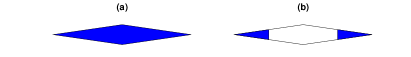
Figure 2: (Color online) Diagrammatic representation of generating functions $\hat{T}_{n}(x)$ (a) and $\hat{S}_{n}(x,y$) (b). Filled areas indicate connected components that either connect to both end nodes [$\hat{T}_{n}(x)$] or connect to a single end node [$\hat{S}_{n}(x,y)$].

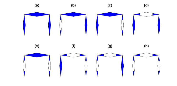
Figure 3: (Color online) The diagrams coming from a single $m$-polygon added at iteration $n+1-j$ with $m=4$ are shown. These diagrams represent terms that contribute to $\hat{T}_{n+1}(x)$ and $\hat{S}_{n+1}(x,y)$. Diagram (a) contributes exclusively to $\hat{T}_{n+1}(x)$ with a term $x^{2}\hat{T}^{3}_{j}$, diagrams (b)-(h) contribute both to $\hat{T}_{n+1}(x)$ and $\hat{S}_{n+1}(x,y)$. The diagrams (b)-(h) contribute to $\hat{T}_{n+1}(x)$ under the assumption that both initial nodes are connected either by the initial link or by polygons added at different generations. The contribution of the diagrams (b)-(h) to $\hat{T}_{n+1}(x)$ are: (b), (c) and (d) $x^{2}\hat{T}^{2}_{j}(x)\hat{S}_{n}(x,x)$; (e) and (h) $\hat{S}^{2}_{j}(x,1)$; (f) and (g) $x\hat{T}_{j}(x)\hat{S}^{2}_{j}(x,1)$. The diagrams (b)-(h) contribute to $\hat{S}_{n+1}(x,y)$ under the assumption that the two initial nodes not connected by the initial link and by any other polygon added at different generations. The contribution of the diagrams (b)-(h) to $\hat{S}_{n+1}(x,y)$ are: (b) $y^{2}\hat{T}^{2}_{j}(y)\hat{S}_{n}(x,y)$; (c) $x^{2}\hat{T}^{2}_{j}(x)\hat{S}_{n}(x,y)$; (d) $xy\hat{T}_{j}(x)\hat{T}_{j}(y)\hat{S}_{n}(x,y)$; (e) and (h) $\hat{S}_{j}(x,1)\hat{S}_{j}(y,1)$; (f),$x\hat{T}_{j}(x)\hat{S}_{j}(x,1)\hat{S}_{j}(y,1)$; (g) $y\hat{T}_{j}(y)\hat{S}_{j}(x,1)\hat{S}_{j}(y,1)$.

The generating functions at iteration $n=0$ are given by

$$\hat{T}_{0}(x) = p$$

$$\hat{S}_{0}(x,y) = 1-p,$$ (16)

because initially the two nodes can be either connected by a link (which occurs with probability $p$) or not connected by a link (which occurs with probability $1-p$). In both cases the two initial nodes are not connected to any other node so $t_{n}(0)=p$, and $t_{n}(\ell)=0,$ for all $\ell>0$; similarly $s_{n}({0,0})=1-p$ and $s_{n}(\ell,\overline{\ell})=0$ for all $(\ell,\overline{\ell})\neq(0,0)$.

Our aim is to write a set of recursive equations for $\hat{T}_{n+1}(x)$ and $\hat{S}_{n+1}(x,y)$ expressing the generating functions at iteration $n+1$ given the expression of the generating functions at previous generations. To this end we follow the diagrammatic representation of the generating functions $\hat{T}_{n}(x)$ and $\hat{S}_{n}(x,y)$, already introduced in Refs.  Boettcher et al. (2012); Kryven et al. (2019); Bianconi et al. (2019). In particular we represent $\hat{T}_{n}(x)$ and $\hat{S}_{n}(x,y)$ with the diagrams presented in Fig.  2.

At iteration $n+1$ the initial link will be incident to $n+1$ polygons added subsequently at each iteration. The polygon added at iteration $n+1-j$ with $0\leq j\leq n$ has links whose statistical properties are equivalent to the one of the initial link at iteration $j$. If we consider a single polygon added at iteration $n+1-j$, its links will connect the two initial nodes to other nodes of the cell complex added at later generations, and these nodes will not be reachable by following links that branch out from other polygons. The polygon added at iteration $n+1-j$ will contribute to the generating functions $\hat{T}_{n+1}(x)$ and $\hat{S}_{n+1}(x,y)$ with terms that can be expressed diagrammatically as described in Fig.  $\ref{Fig:diagram}(a)$ for a $m$-polygon with $m=4$. Only one of these diagrams, i.e., the diagram corresponding to $x^{m-2}T_{j}^{m-1}$ (diagram (a) in Fig.  3) will guarantee connectivity of the two end nodes. Therefore the diagram in Fig.  $\ref{Fig:diagram}(a)$ and its counterpart diagrams for polygons of different number of sides, cannot contribute to $\hat{S}_{n}(x,y)$. However since the initial link at iteration $n$ is connected to $n$ polygons and connectivity can be guaranteed by the initial link or, when this link is removed, by any one of the polygons connected to the initial link, all diagrams contribute to $\hat{T}_{n+1}(x)$.

In order to calculate the generating function $\hat{S}_{n}(x,y)$ we need to impose that the initial nodes are not directly connected, i.e., for every polygons we need to consider only the contributions from diagrams that do not guarantee connectivity (diagrams (b)-(h) of Fig.  3). In this way, for a deterministic pseudo-fractal cell complex we obtain

$$\hat{S}_{n+1}(x,y)=(1-p)\prod_{j=0}^{n}\left[\sum_{r=0}^{m-2}x^{r}y^{m-2-r}\hat{T}_{j}^{r}(x)\hat{S}_{j}(x,y)\hat{T}_{j}^{m-2-r}(y)+\sum_{s=0}^{m-3}\sum_{r=0}^{s}x^{r}y^{s-r}\hat{T}_{j}^{r}(x)\hat{S}_{j}(x,1)\hat{S}_{j}(y,1)\hat{T}_{j}^{s-r}(y)\right].$$ (17)

The derivation of the recursive equation for $\hat{T}_{n+1}(x)$ is slightly more complex. In fact, in order to guarantee that $\hat{T}_{n+1}(x)$ is the generating function of the connected component connected to both initial nodes, we need to impose connectivity. As noted before, it is sufficient that the initial link guarantees connectedness or, when this link is removed, it is sufficient that a single polygon contributes for the connectedness of the two initial nodes. Therefore we express $T_{n+1}(x)$ as the difference between two terms. The first term considers, for each polygon the contribution of all diagrams (the one that guarantee connectedness and the one that do not). The second term considers for each polygons only the terms that do not guarantee connectedness, i.e. removes from the first term the contribution coming from disconnected configurations. In this way for a deterministic pseudo-fractal cell complex we obtain,

$$\hat{T}_{n+1}(x)=\prod_{j=0}^{n}\left[x^{m-2}\hat{T}_{j}^{m-1}(x)+(m-1)x^{m-2}\hat{T}_{j}^{m-2}(x)S_{j}(x,x)+\sum_{s=0}^{m-3}(s+1)x^{s}\hat{T}_{j}^{s}(x)\hat{S}_{j}(x,1)\hat{S}_{n}(1,x)\right]$$

$$\hskip 25.60747pt-(1-p)\prod_{j=0}^{n}\left[(m-1)x^{m-2}\hat{T}_{j}^{m-2}(x)S_{j}(x,x)+\sum_{s=0}^{m-3}(s+1)x^{s}\hat{T}_{j}^{s}(x)\hat{S}_{j}(x,1)\hat{S}_{j}(1,x)\right].$$

For a random pseudo-fractal cell-complex we can generalize these equations obtaining for $\hat{T}_{n}(x)$ and $\hat{S}_{n}(x,y)$ the recursion

$$\hat{S}_{n+1}(x,y)=(1-p)\prod_{j=0}^{n}\left\{\sum_{m\geq 3}q_{m}\left[\sum_{r=0}^{m-2}x^{r}y^{m-2-r}\hat{T}_{j}^{r}(x)\hat{S}_{j}(x,y)\hat{T}_{j}^{m-2-r}(y)+\sum_{s=0}^{m-3}\sum_{r=0}^{s}x^{r}y^{s-r}\hat{T}_{j}^{r}(x)\hat{S}_{j}(x,1)\hat{S}_{j}(y,1)\hat{T}_{j}^{s-r}(y)\right]\right\},$$

$$\hat{T}_{n+1}(x)=\prod_{j=0}^{n}\left\{\sum_{m\geq 3}q_{m}\left[x^{m-2}\hat{T}_{j}^{m-1}(x)+(m-1)x^{m-2}\hat{T}_{j}^{m-2}(x)S_{j}(x,x)+\sum_{s=0}^{m-3}(s+1)x^{s}\hat{T}_{j}^{s}(x)\hat{S}_{j}(x,1)\hat{S}_{n}(1,x)\right]\right\}$$

$$\hskip 25.60747pt-(1-p)\prod_{j=0}^{n}\left\{\sum_{m\geq 3}q_{m}\left[(m-1)x^{m-2}\hat{T}_{j}^{m-2}(x)S_{j}(x,x)+\sum_{s=0}^{m-3}(s+1)x^{s}\hat{T}_{j}^{s}(x)\hat{S}_{j}(x,1)\hat{S}_{j}(1,x)\right]\right\},$$

with initial conditions $\hat{T}_{0}(x)=1-\hat{S}_{0}(x,y)=p$.

We are particularly interested in the generating function $\hat{T}_{n}(x)$ whose derivative calculated for $x=1$ gives the expected size of the giant component. The generating function $\hat{T}_{n+1}(x)$ depends on the generating functions $\hat{T}_{j}(x)$ and the functions $\hat{\Sigma}_{j}(x)=\hat{S}_{j}(x,x)$, and $\hat{S}_{j}(x)=\hat{S}_{j}(1,x)$ at iterations $0\leq j\leq n$. From the above equations for $\hat{T}_{n+1}(x)$ and $S_{n+1}(x,y)$ we can deduce directly the set of recursive equations for $\hat{T}_{n+1}(x)$, $\hat{\Sigma}_{n+1}(x)$, and $\hat{S}_{n+1}(x)$ which read

$$\hat{T}_{n+1}(x) = \prod_{j=0}^{n}\left\{\sum_{m\geq 3}q_{m}\left[x^{m-2}\hat{T}_{j}^{m-1}(x)+(m-1)x^{m-2}\hat{T}^{m-2}_{j}(x)\Sigma_{j}(x)+\left(\sum_{i=0}^{m-3}(i+1)x^{i}\hat{T}_{j}^{i}(x)\right)S_{j}^{2}(x)\right]\right\}$$

$$-(1-p)\prod_{j=0}^{n}\left\{\sum_{m\geq 3}q_{m}\left[(m-1)x^{m-2}\hat{T}_{j}^{m-2}(x)\Sigma_{j}(x)+\left(\sum_{i=0}^{m-3}(i+1)x^{i}\hat{T}_{j}^{i}(x)\right)S^{2}_{j}(x)\right]\right\},$$

$$\hat{\Sigma}_{n+1}(x) = (1-p)\prod_{j=0}^{n}\left\{\sum_{m\geq 3}q_{m}\left[(m-1)x^{m-2}\hat{T}_{j}^{m-2}(x)\Sigma_{j}(x)+\left(\sum_{i=0}^{m-3}(i+1)x^{i}\hat{T}_{j}^{i}(x)\right)S^{2}_{j}(x)\right]\right\},$$

$$\hat{S}_{n+1}(x) = (1-p)\prod_{j=0}^{n}\left\{\sum_{m\geq 3}q_{m}\left[\left(\sum_{i=0}^{m-2}x^{i}\hat{T}_{j}^{i}(x)\right)S_{j}(x)\right]\right\}.$$ (18)

These equations differ significantly from the corresponding equations valid for two-dimensional hyperbolic manifolds Boettcher et al. (2012); Kryven et al. (2019) and for branched simplicial complexes Bianconi et al. (2019). In fact these equations for $\hat{T}_{n+1}(x),\hat{\Sigma}_{n+1}(x)$ and $\hat{S}_{n+1}(x)$ depend on the entire RG flow of the process, i.e., their left hand side if a function of all $\hat{T}_{j}(x)$, $\hat{\Sigma}_{j}(x)$ and $\hat{S}_{j}(x)$ all previous iterations $j$ with $0\leq j\leq n$.

This apparent complication of the obtained equations can be removed by introducing an auxiliary function $K_{n+1}(x)$ (see for instance a similar trick used for the Gaussian model in Refs. Bianconi and Dorogovstev (2020); Reitz and Bianconi (2020)). In order to show this let us rewrite the Eqs. (18) as

$$\hat{T}_{n+1}(x) = \hat{K}_{n+1}(x)-\hat{\Sigma}_{n+1}(x)$$

$$\hat{K}_{n+1}(x) = \prod_{j=0}^{n}\left\{\sum_{m\geq 3}q_{m}\left[x^{m-2}\hat{T}_{j}^{m-1}(x)+(m-1)x^{m-2}\hat{T}^{m-2}_{j}(x)\Sigma_{j}(x)+\left(\sum_{i=0}^{m-3}(i+1)x^{i}\hat{T}_{j}^{i}(x)\right)S_{j}^{2}(x)\right]\right\}$$

$$\Sigma_{n+1}(x) = (1-p)\prod_{j=0}^{n}\left\{\sum_{m\geq 3}q_{m}\left[(m-1)x^{m-2}\hat{T}_{j}^{m-2}(x)\Sigma_{j}(x)+\left(\sum_{i=0}^{m-3}(i+1)x^{i}\hat{T}_{j}^{i}(x)\right)S^{2}_{j}(x)\right]\right\},$$

$$S_{n+1}(x) = (1-p)\prod_{j=0}^{n}\left\{\sum_{m\geq 3}q_{m}\left[\left(\sum_{i=0}^{m-2}x^{i}\hat{T}_{j}^{i}(x)\right)S_{j}(x)\right]\right\},$$ (19)

with initial conditions $\hat{T}_{0}(x)=p,\hat{\Sigma}_{0}(x)=\hat{S}_{0}(x)=1-p,\hat{K}_{0}(x)=1$. This latter system of equations can be expressed by a set of iterative equations between the variables at iteration $n$ and the variable at iteration $n+1$, i.e.,

$$\hat{T}_{n+1}(x) = \hat{K}_{n+1}(x)-\hat{\Sigma}_{n+1}(x)$$

$$\hat{K}_{n+1}(x) = \hat{K}_{n}(x)\left\{\sum_{m\geq 3}q_{m}\left[x^{m-2}\hat{T}_{n}^{m-1}(x)+(m-1)x^{m-2}\hat{T}^{m-2}_{n}(x)\Sigma_{n}(x)+\left(\sum_{i=0}^{m-3}(i+1)x^{i}\hat{T}_{n}^{i}(x)\right)S_{n}^{2}(x)\right]\right\}$$

$$\Sigma_{n+1}(x) = \Sigma_{n}(x)\left\{\sum_{m\geq 3}q_{m}\left[(m-1)x^{m-2}\hat{T}_{n}^{m-2}(x)\Sigma_{n}(x)+\left(\sum_{i=0}^{m-3}(i+1)x^{i}\hat{T}_{n}^{i}(x)\right)S^{2}_{n}(x)\right]\right\},$$

$$S_{n+1}(x) = S_{n}(x)\left\{\sum_{m\geq 3}q_{m}\left[\left(\sum_{i=0}^{m-2}x^{i}\hat{T}_{n}^{i}(x)\right)S_{n}(x)\right]\right\}.$$ (20)

As we will see in the next section, this recursive set of equations will turn out to be particular useful for evaluating the expected size of the giant component.

III.3 Order parameter

The order parameter of link percolation is the fraction of nodes $P_{\infty}$ that in thermodynamic limit belongs to the giant component, i.e.,

$$P_{\infty} = \lim_{n\to\infty}\frac{M_{n}}{\overline{N}_{n}}.$$ (21)

where $M_{n}$ is the expected size of the giant component connected to the two initial nodes of the cell complex. The value of $M_{n}$ can be derived from the generating function $\hat{T}_{n}(x)$ by derivation, i. e.,

$$M_{n}=\left.\frac{d\hat{T}_{n}(x)}{dx}\right|_{x=1}.$$ (22)

In order to obtain $M_{n}$ we rewrite Eqs. (20) in terms of the vector

$${\bf V}_{n}(x) = \left(V_{n}^{1}(x),V_{n}^{2}(x),V_{n}^{3}(x),V^{4}_{n}(x)\right)^{\top}$$ (23)

$$= \left(\hat{T}_{n}(x),\hat{K}_{n}(x),\hat{\Sigma}_{n}(x),\hat{S}_{n}(x)\right)^{\top},$$

as

$${\mathbf{V}}_{n+1}^{s}(x)={\mathbf{F}_{n}}(\{\mathbf{V}_{n}(x)\},x).$$ (24)

By using this notation, we note that the derivative of ${\bf V}_{n+1}(x)$ calculated at $x=1$ follows

$$\left.\frac{d{\mathbf{V}}_{n+1}(x)}{dx}\right|_{x=1}={\bf J}_{n}\left.\frac{d{\bf V}_{n}^{p}(x)}{dx}\right|_{x=1}+\left.\frac{\partial{\bf F}_{n}^{s}}{\partial x}\right|_{x=1},$$ (25)

where ${\bf J}_{n}$ indicates the Jacobian matrix of the system of Eqs. (24). The initial condition of Eq. (25) is ${\dot{\bf V}}_{0}={\bf 0}$ obtained by taking into consideration that the initial nodes are not counted. In order to evaluate Eqs. (24) we need to provide an explicit expression of the Jacobian matrix ${\bf J}_{n}$ whose elements are given by

$$[\left.{\bf J}_{n}]_{ij}=\frac{\partial{F}_{n+1}^{i}}{\partial{V}_{n}^{j}(x)}\right|_{x=1}.$$ (26)

Let us we indicate with $T_{n}=\hat{T}_{n}(1)$, $\Sigma_{n}=\Sigma_{n}(1)$ $S_{n}=\hat{S}_{n}(1)$ and $K_{n}=\hat{K}_{n}(1)$ that by definition satisfy $T_{n}=1-S_{n}=1-\Sigma_{n}$ and ${K}_{n}=1$.

By direct calculation of the Jacobian ${\bf J}_{n}$ we notice that ${\bf J}_{n}$ can be expressed as a function of $Q(T_{n})$ and $H(T_{n})$ with $Q(T)$ given by Eq.  (5) and $H(T)$ given by

$$H(T) = \sum_{m\geq 3}q_{m}\sum_{i=0}^{m-2}T^{i}.$$ (27)

In fact, by using the following two relations

$$\left(1-T_{n}\right)\sum_{i=0}^{m-3}i(i+1)T_{n}^{i-1}=$$

$$2\sum_{i=0}^{m-3}(i+1)T_{n}^{i}-(m-1)(m-2)T_{n}^{m-3},$$ (28)

and

$$\left(1-T_{n}\right)\sum_{i=0}^{m-3}(i+1)T_{n}^{i}=\sum_{i=0}^{m-2}T_{n}^{i}-(m-1)T_{n}^{m-2},\$$

and using $T_{n}=1-S_{n}=1-\Sigma_{n}$, $K_{n}=1$, a direct calculation show that ${\bf J}_{n}$ is given by

$${\bf J}_{n}=\left(\begin{array}[]{cccc}Q^{\prime}(T_{n})+2T_{n}[H(T_{n})-Q^{\prime}(T_{n})]&1&T_{n}Q^{\prime}(T_{n})-S_{n}H(T_{n})&2T_{n}[H(T_{n})-Q^{\prime}(T_{n})]\\ Q^{\prime}(T_{n})+2[H(T_{n})-Q^{\prime}(T_{n})]&1&Q^{\prime}(T_{n})&2[H(T_{n})-Q^{\prime}(T_{n})]\\ 2S_{n}[H(T_{n})-Q^{\prime}(T_{n})]&0&S_{n}[H(T_{n})+Q^{\prime}(T_{n})]&2S_{n}[H(T_{n})-Q^{\prime}(T_{n})]\\ S_{n}[H(T_{n})-Q^{\prime}(T_{n})]&0&0&2S_{n}H(T_{n})\end{array}\right).$$ (33)

Similarly the inhomogeneous term can be expressed as

$$\frac{\partial{\bf F}_{n}}{\partial x}=\left(\begin{array}[]{c}(m-2)Q(T_{n})+2T_{n}^{2}(H(T_{n})-Q^{\prime}(T_{n}))\\ (m-2)Q(T_{n})+2T_{n}[H(T_{n})-Q^{\prime}(T_{n})]\\ 2T_{n}S_{n}[H(T_{n})-Q^{\prime}(T_{n})]\\ T_{n}S_{n}[H(T_{n})-Q^{\prime}(T_{n})]\end{array}\right).$$ (38)

Since we have now an explicit expression for both ${\bf J}_{n}$ and ${\partial{\bf F}_{n}}/{\partial x}$, we can numerically integrate Eq. (24) finding the number of nodes $M_{n}$ in the giant component of pseudo-fractal cell complexes for any value of $n$ (numerical precision permitting). However we also want to have some analytical predictions of the critical properties of link percolation. To this end we notice that for $n>0$ and $T_{n}<1$ the non-homogeneous term ${\partial{\bf F}_{n}}/{\partial x}$ is subleading with respect to the homogeneous one in Eq.  (24). However for $n=0$ the homogeneous term vanishes due to the initial condition $\dot{\bf V}_{0}={\bf 0}$ so therefore the non-homogeneous term cannot be neglected. Therefore we can express $\dot{\bf V}_{n+1}$ as

$$\dot{\bf V}_{n+1}\simeq{\mathcal{A}}_{n}\prod_{n^{\prime}=1}^{n}\lambda_{n^{\prime}}{\bf u}_{n},$$ (39)

where $\lambda_{n}$ and ${\bf u}_{n}$ are the largest eigenvalue and the corresponding left eigenvector of the Jacobian matrix ${\mathbf{J}}_{n}$ and ${\mathcal{A}}_{n}$ is given by

$${\mathcal{A}}_{n}=\left(\prod_{n^{\prime}=2}^{n}\braket{{\bf v}_{n^{\prime}}}{{\bf u}_{n^{\prime}-1}}\right)\braket{{\bf v}_{1}}{\dot{\bf V}_{1}},$$ (40)

with $\dot{\bf V}_{0}={\partial{\bf F}_{0}}/{\partial x}$ and ${\bf v}_{n}$, indicating the right eigenvector corresponding to the largest eigenvalue of the Jacobian ${\bf J}_{n}$.

Using Eq.  (33) we can directly calculate the largest eigenvalue $\lambda_{n}$ of the Jacobian matrix ${\bf J}_{n}$ which is given by

$$\lambda_{n}=\frac{1}{2}\left[\hat{K}(T_{n})+\sqrt{\hat{\Delta}(T_{n})}\right],$$ (41)

where $\hat{\Delta}(T_{n})$ and $\hat{K}(T_{n})$ are given by

$$\hat{K}(T_{n}) = (1-2T)Q^{\prime}(T_{n})+2H(T_{n})+1,$$ (42)

$$\hat{\Delta}(T_{n}) = \left[\hat{K}(T_{n})\right]^{2}+8(T-1)\left[H^{2}(T_{n})+Q^{\prime}(T_{n})\right].$$

Note that for $T_{n}\to 1$ then $\lambda_{n}\to\langle{m}\rangle$.

The right eigenvector $\bf v_{n}$ corresponding to the largest eigenvalue of ${\bf J}_{n}$ is given by:

$${\bf v}_{n}=\frac{1}{\mathcal{C}^{R}}\left(\begin{array}[]{c}{\hat{K(T_{n})}-4H(T_{n})(1-T_{n})+\sqrt{\hat{\Delta}(T_{n})}}{2(H(T_{n})-Q^{\prime}(T_{n}))(T_{n}-1)}\\ {\hat{K(T_{n})}-4Q^{\prime}(T_{n})(1-T_{n})+\sqrt{\hat{\Delta}(T_{n})}}\\ -{4(H(T_{n})-Q^{\prime}(T_{n}))(T_{n}-1)}\\ -{2(H(T_{n})-Q^{\prime}(T_{n}))(T_{n}-1)}\end{array}\right)$$ (47)

and the corresponding left eigenvector ${\bf u}_{n}$ is given by:

$${\bf u}_{n}^{L}=\frac{1}{\mathcal{C}^{L}}\left(\begin{array}[]{c}{2H^{3}(T_{n})+4H(T_{n})Q^{\prime}(T_{n})-2Q^{\prime 2}(T_{n})+H^{2}(T_{n})\left[-1-3Q^{\prime}(T_{n})+2T_{n}Q^{\prime}(T_{n})+\sqrt{\hat{\Delta}(T_{n})}\right]}\\ {2H^{2}(T_{n})-2H(T_{n})Q^{\prime}(T_{n})+Q^{\prime}(T_{n})\left[1-Q^{\prime}(T_{n})+2T_{n}Q^{\prime}(T_{n})+\sqrt{\hat{\Delta}(T_{n})}\right]}\\ {-2H^{3}(T_{n})+2Q^{\prime 2}(T_{n})+H^{2}(T_{n})\left[-1+Q^{\prime}(T_{n})+2T_{n}Q^{\prime}(T_{n})+\sqrt{\hat{\Delta}(T_{n})}\right]}\\ 4(\left[H(T_{n})-Q^{\prime}(T_{n})\right]\left[H^{2}(T_{n})+Q^{\prime}(T_{n})\right]\end{array}\right),$$ (52)

where $\mathcal{C}^{R}$ and $\mathcal{C}^{L}$ are normalization constants which guarantee that the right and left eigenvectors have absolute value one. Note that the right and left eigenvectors of ${\bf v}_{n}$ and ${\bf u}_{n}$ satisfy by definition

$$\langle{\bf v}_{n}|{\bf u}_{n}\rangle=1.$$ (53)

From Eqs.  (39) and (22) it follows that the expected number of nodes $M_{n+1}$ in the giant component can be expressed as

$${M}_{n+1}\simeq{\mathcal{A}}_{n}\prod_{n^{\prime}=1}^{n}\lambda_{n^{\prime}}{u}_{n}^{1},$$ (54)

where $u_{n}^{1}$ indicates the first element of the vector ${\bf u}_{n}$.

In Sec.  V we will use Eq.  (54) to derive the critical properties of link percolation on the pseudo-fractal cell complexes.

IV RG flow

In this section we study the RG flow described by Eq. (6) that we rewrite here for convenience

$$T_{n+1}=1-(1-T_{n})(1-Q(T_{n})),$$ (55)

with initial condition $T_{0}=p$. By defining the auxiliary variable

$$y_{n}=-\ln(1-T_{n})$$ (56)

the RG flow described by Eq.  (55) can be written as

$$y_{n+1}=G(y_{n})=y_{n}-\ln(1-Q(1-e^{-y_{n}})).$$ (57)

For $p\ll 1$, i.e., close to $p_{c}=0$ we can develop Eq. (57) close to $T=T_{c}=0$, $y_{c}=0$. Stopping at the first relevant term in the expansion of $y_{n+1}-y_{n}$ we obtain

$$y_{n+1}-y_{n}=q_{\overline{m}}y_{n}^{\overline{m}-1},$$ (58)

with initial condition $y_{0}=-\ln(1-p)$. Note that in Eq.  (58), $\overline{m}$ indicates the minimum value of $m$ for which $q_{m}>0$. By going in the continuous limit and substituting $y_{n}$ with a function $y(n)$, Eq. (58) can be written as

$$\frac{dy}{dn}=q_{\overline{m}}y^{\overline{m}-1}.$$ (59)

By integrating this equation from $0$ up to $n$ we get

$$y=y_{0}\left[1-n/n_{c}\right]^{-1/(\overline{m}-2)},$$ (60)

with

$$n_{c}=\left[(\overline{m}-2)|\ln(1-p)|^{\overline{m}-2}q_{\overline{m}}\right]^{-1}.$$ (61)

In particular $y$ diverges at a finite value of $n=n_{c}$.

From Eq.  (60) using

$$1-T_{n}\simeq e^{-y_{n}}$$ (62)

we get the the asymptotic scaling valid for $y\ll 1$ and $p\ll 1$

$$1-T_{n}=(1-p)^{\theta_{n}}$$ (63)

with

$$\theta_{n} = \left[1-(\overline{m}-2)|\ln(1-p)|^{\overline{m}-2}q_{\overline{m}}n\right]^{-1/(\overline{m}-2)}.$$ (64)

For $n\ll n_{c}$ we can made a further approximation and express $\theta_{n}$ as

$$\theta_{n}\simeq\exp\left[q_{\overline{m}}p^{\overline{m}-2}n\right].$$ (65)

Therefore for $n\ll n_{c}$

$$y_{n}=y_{0}\exp\left[q_{\overline{m}}p^{\overline{m}-2}n\right],$$ (66)

with $y_{0}=|\ln(1-p)|$.

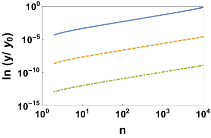
Figure 4: (Color online) The RG flow is represented by plotting $\ln(y/y_{0})$ (where $y_{0}=-\ln(1-p)$) versus $n$ for $p=5\times 10^{-5}$ with $m=3$ (blue solid line) $m=4$ (orange dashed line) and $m=5$ (green dot-dashed line).

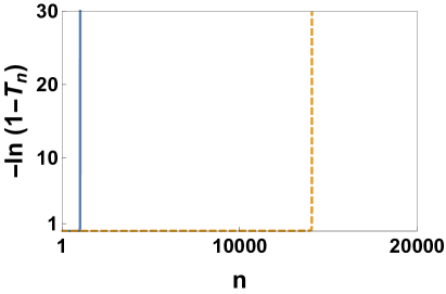
Figure 5: (Color online) The RG flow is shown by plotting the value $y_{n}=-\ln(1-T_{n})$ where $T_{n}$ is the percolation probability, versus $n$ for fixed value of $p$. The solid (blue) line indicates the RG flow for the deterministic pseudo-fractal simplicial complex with $m=3$ and $p=10^{-3}$, the dashed (orange) line indicates the RG flow for the deterministic pseudo-fractal cell complex with $m=4$ and $p=6\times 10^{-3}$. The divergence of $y_{n}$ occurring at a value of $n$ of the order of magnitude of $n_{c}$ is clearly noticeable, indicating a discontinuity of $T_{n}$ reaching the value $T_{n}=1$ discontinuously.

In Fig.  4 we show the very good agreement between the numerically integrated value of $y_{n}$ and the expression given by Eq.  (66) for $n\ll n_{c}$.

Finally we notice that although Eq.  (60) is obtained in the limit $y\ll 1$ we can see from numerical integration of the RG flow that $y$ retains the structure

$$y=y_{0}f(n/n_{c}).$$ (67)

Although the functional form of $f(n/n_{c})$ obtained in the expansion for $0<y\ll 1$ (which can be deducted from Eq.  (60)) is not exact close to $n\simeq n_{c}$, from this expansion we can deduce that $y$ diverges for a finite value of $n$ of the order of $n_{c}$. In correspondence of this divergence the linking probability $T_{n}$ jumps to $T_{n}=1$ (see Fig.  5).

V Critical properties of the order parameter

V.1 Critical region

We are interested in characterizing the properties of the order parameter

$$P_{\infty} = \lim_{n\to\infty}\frac{M_{n}}{\overline{N}_{n}}.$$ (68)

in the critical region, i.e., close to the percolation threshold $p_{c}=0$ taking $0<p\ll 1$. To this end we first discuss the properties of the expected number of nodes $M_{n}$ in the giant component when the pseudo-fractal cell complex has evolved up to iteration $n$. According to the derivation obtained in Sec.  III.3, using Eq.  (54), $M_{n}$ can be approximated as

$$M_{n}\simeq{\mathcal{A}}_{n-1}\prod_{n^{\prime}=1}^{n-1}\lambda_{n^{\prime}}{u}_{n}^{1},$$ (69)

where ${\mathcal{A}}_{n}$ is given by Eq.  (40), which can be written also as

$${\mathcal{A}}_{n}={\mathcal{D}}_{n}\braket{{\bf v}_{1}}{\dot{\bf V}_{1}},$$ (70)

where ${\mathcal{D}}_{n}$ is given by

$${\mathcal{D}}_{n}=\prod_{n^{\prime}=2}^{n}\braket{{\bf v}_{n^{\prime}}}{{\bf u}_{n^{\prime}-1}}$$ (71)

For $p\simeq p_{c}$, ${\mathcal{D}}_{n}$ is in first approximation independent of $n$ and approximately equal to one, as the right and left eigenvectors will change slowly with $n$ and by definition Eq.  (53) is satisfied. Therefore Eq.  (69) can be written as

$$M_{n}\simeq\braket{{\bf v}_{1}}{\dot{\bf V}_{1}}\prod_{n^{\prime}=1}^{n-1}\lambda_{n^{\prime}}{u}_{n}^{1}.$$ (72)

V.2 Critical expansions

Our major goal is to study the critical behavior of the order parameter $P_{\infty}$ (given by Eq.  (68)) depending on the scaling of the expected number of of nodes $M_{n}$ (whose leading behavior is given by Eq. (72)) in the pseudo-fractal simplicial complex with the number of iterations $n$.

To this end in this paragraph we will investigate the scaling of $\lambda_{n}$ with $n$ for $0<p\ll 1$ and we will investigate the scaling of the other factors $\braket{{\bf v}_{1}}{\dot{\bf V}_{1}}$ and ${u}_{n}^{1}$ present in Eq.  (72) with $p$.

The leading eigenvalues $\lambda_{n}$ of the Jacobian matrix ${\bf J}_{n}$ is expressed according to Eq.  (41) as a function of $H(T_{n})$ and $Q(T_{n})$. For $y_{n}=-\ln(1-T_{n})\ll 1$ we can expand both $H(T_{n})=H(1-e^{-y_{n}})$ and $Q^{\prime}(T_{n})=Q^{\prime}(1-e^{-y_{n}})$ getting

$$Q^{\prime}(1-e^{-y_{n}}) = q_{\overline{m}}(\overline{m}-1)y_{n}^{\overline{m}-2}+\mathcal{O}(y^{\overline{m}-1}_{n},)$$

$$H(1-e^{-y_{n}}) = 1+y_{n}+O(y_{n}^{2}).$$ (73)

where $\overline{m}$ indicates the smaller value of $m$ for which $q_{m}>0$. Using this expansion in the Eq.  (41) for the maximum eigenvalue $\lambda_{n}$ of the Jacobian matrix, we get

$$\lambda_{n}=2(1+y_{n})+O(y_{n}^{2})$$ (74)

For $y_{n}\ll 1$ also the inhomogeneous term $\partial{\bf F}_{n}/{\partial x}$ can be expanded to give

$$\frac{\partial{\bf F}_{n}}{\partial x}\simeq\left(\begin{array}[]{c}(2+q_{3})y_{n}^{2}\\ 2y_{n}\\ 2y_{n}\\ y_{n}\end{array}\right),$$ (79)

For $n=0$ where the homogeneous term vanishes due to the trivial initial condition $\dot{\bf V}_{0}={\bf 0}$ and the inhomogeneous term has the leading behavior

$$\dot{\bf V}_{1}=\frac{\partial{\bf F}_{0}}{\partial x}\simeq\left(\begin{array}[]{c}(2+q_{3})p^{2}\\ 2p\\ 2p\\ p\end{array}\right).$$ (84)

Moreover the leading term of ${\bf v}_{1}$ is

$${\bf v}_{1}\simeq\frac{1}{6-4p/3}((1+p),(1-p),(-1+p),2).$$ (85)

Therefore for $p\ll 1$ we have that $\braket{{\bf v_{1}}}{\dot{\bf V}_{1}}$ scales linearly with $p$. In particular

$$\braket{{\bf v_{1}}}{\dot{\bf V}_{1}}\simeq\frac{p}{3}.$$ (86)

Finally we observe that for $n\gg 1$ we have $T_{n}\simeq 1$ and the right eigenvector corresponding to the largest eigenvalue scales like

$${\bf u}_{n}=(1,1,0,0)^{\top}.$$ (87)

By considering the scaling relations determined by Eq.  (86) and Eq.  (87) in Eq.  (72) we obtain that for $n\gg 1$ the fraction of nodes $M_{n}$ in the giant component obeys

$$M_{n}\propto p\prod_{n^{\prime}=1}^{n-1}\lambda_{n^{\prime}}.$$ (88)

with $\lambda_{n}$ following Eq. (74) for $y_{n}\ll 1$.

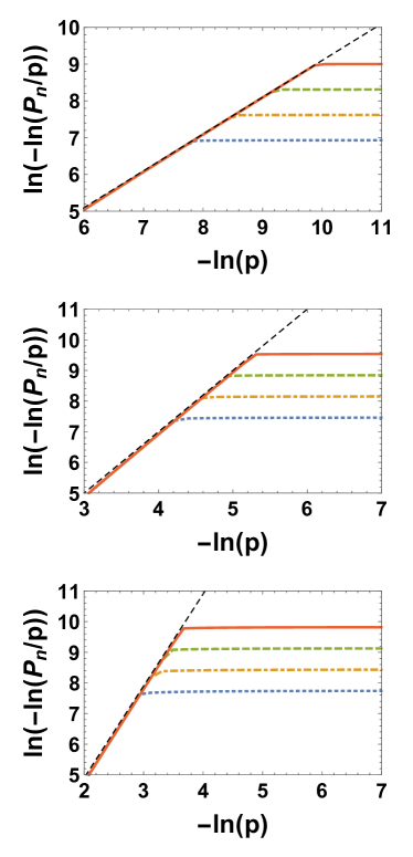
Figure 6: (Color online) The scaling of the order parameter $P_{n}$ is shown a as function of $p$ for the deterministic pseudo-fractal simplicial and cell complexes with $m=3$ (top panel), $m=4$ (central panel) and $m=5$ (bottom panel). The order parameter $P_{n}$ is shown for different values of $n=20000,10000,5000,2500$ indicated with solid (red), dashed (green) dot-dashed (orange) and dotted (blue) thick lines. The predicted scaling of the order parameter in the infinite network limit is indicated with the thin dashed (black) line.

V.3 Critical scaling of the order parameter

In this paragraph we derive the asymptotic behavior of the order parameter $P_{\infty}$ given by Eq.  (68) close to the percolation threshold $p_{c}=0$. By approximating $M_{n}$ with Eq. (88) the order parameter $P_{\infty}$ given by Eq.  (68) can be easily shown to obey for $0<p\ll 1$

$$P_{\infty} \propto p\lim_{n\to\infty}\frac{1}{\overline{N}_{n}}\prod_{n^{\prime}=1}^{n}\lambda_{n^{\prime}}$$ (89)

$$= p\exp\left[-\ln\langle{m}\rangle\int_{0}^{\infty}dn(1-\psi_{n})\right]$$

where $\psi_{n}$ is defined as

$$\psi_{n}=\frac{\ln\lambda_{n}}{\ln\langle{m}\rangle}.$$ (90)

Using for $\lambda_{n}$ the expansion given by Eq. (74) $\psi_{n}$ can be expanded to give

$$\psi_{n}=\frac{\ln\lambda_{n}}{\ln\langle{m}\rangle}=\frac{\ln 2}{\ln\langle{m}\rangle}+\frac{y_{n}}{\ln\langle{m}\rangle}+O(y_{n}^{2}).$$ (91)

Therefore in the continuous limit for $n$ we get

$$1-\psi\simeq 1-\frac{\ln 2}{\ln\langle{m}\rangle}-\frac{y}{\ln m}$$ (92)

with the function $y(n)$ given by the scaling function Eq.  (67) and diverging for $n={n_{c}}$. At a value of $n\sim n_{c}$, $T_{n}$ jumps to $T_{n}=1$, $\lambda_{n}=\left\langle{m}\right\rangle$. Consequently we have that $1-\psi_{n}$ will also have a discontinuity at $n_{c}$, i.e.,

$$1-\psi_{n}=\left\{\begin{array}[]{ccc}f_{\psi}(\hat{n}/n_{c})&\mbox{for}&n<n_{c}\\ 0&\mbox{for}&n>n_{c}\end{array}.\right.$$ (95)

where $f_{\psi}(x)$ is a scaling function. Using this expression in Eq.  (89) we obtain

$$P_{\infty} \propto p\exp\left[-\ln\langle{m}\rangle\int_{0}^{\infty}dn(1-\psi_{n})\right]$$ (96)

$$= p\exp\left[-\ln\langle{m}\rangle\int_{0}^{\hat{n}_{c}}d\hat{n}f_{\psi}(\hat{n}/n_{c})\right]$$

By changing the variable of integration from $n$ to $x=n/n_{c}$ we obtain

$$P_{\infty} \propto p\exp\left[-{n_{c}}\ln\langle{m}\rangle\int_{0}^{1}dxf_{\psi}(x)\right]$$ (97)

Finally using the expression for $n_{c}$ given by Eq.  (61), by indicating with $\alpha$ the constant

$$\alpha=\frac{\ln\langle{m}\rangle}{(\overline{m}-2)q_{\overline{m}}}\int_{0}^{1}f_{\psi}(x)dx,$$ (98)

we obtain

$$P_{\infty}\propto p\exp\left(-\frac{\alpha}{|\ln(1-p)|^{\overline{m}-2}}\right).$$ (99)

Because in the critical region $p\ll 1$, it follows that $P_{\infty}$ follows the asymptotic scaling

$$P_{\infty}\propto p\exp(-{\alpha}/{p^{\overline{m}-2}}).$$ (100)

This scaling can be validated by numerically integrating Eq.  (25) and using the finite size scaling of $P_{n}$ defined as the fraction of nodes in the giant component of a pseudo-fractal cell complexes evolved up to iteration $n$, i.e.,

$$P_{n}=\frac{M_{n}}{\overline{N}_{n}}.$$ (101)

Our numerical results shown in Fig.  6 clearly demonstrates that if $n>n_{c}$ (where $n_{c}$ is a function of $p$ defined by Eq.  (61)) then $P_{n}$ follows the asymptotic scaling defined in Eq.  (100). However if $n<n_{c}$, then $P_{n}$ saturates to a constant value. This phenomenology is in perfect agreement with our theoretical understanding of the critical properties of link percolation on pseudo-fractal cell complexes.

VI Conclusions

In this work we have studied the nature of the link percolation transition in pseudo-fractal simplicial and cell complexes. The pseudo-fractal generalized networks under study include deterministic and random cell complexes, made by gluing together $m$-polygons with the same number of sides $m$ or with random number of sides $m$ drawn from a $q_{m}$ distribution. All these generalized network topologies display a link percolation transition at $p_{c}=0$. However the critical behavior of the order parameter depends on the topology of the generalized network structure. For deterministic pseudo-fractal simplicial complexes ($m=3$) we confirm the results of Ref.  Dorogovtsev (2003) showing that the order parameter is exponentially suppressed by a term $1/p$ and we predict an additional modulation of the order parameter by a factor $p$. For deterministic pseudo-fractal cell complexes with $m>3$ we show that the exponential suppression is more severe than for simplicial complexes and decays as $1/p^{m-2}$. Finally for random cell complexes we show that the critical behavior is dominated by the smallest value of $m$, $\overline{m}$ for which $q_{m}>0$. This work shows clearly that the dynamical processes defined on simplicial complexes and their cell complex counterpart might be significantly different, emphasizing the important role that network topology and geometry have on dynamical processes.

References

- Bianconi (2015) G. Bianconi, EPL (Europhys. Lett.) 111, 56001 (2015).
- Salnikov et al. (2018) V. Salnikov, D. Cassese, and R. Lambiotte, Euro. J. Phys. 40, 014001 (2018).
- Giusti et al. (2016) C. Giusti, R. Ghrist, and D. S. Bassett, J. Computational Neuroscience 41, 1 (2016).
- Petri et al. (2014) G. Petri, P. Expert, F. Turkheimer, R. Carhart-Harris, D. Nutt, P. J. Hellyer, and F. Vaccarino, J. Royal Society Interface 11, 20140873 (2014).
- Reimann et al. (2017) M. W. Reimann, M. Nolte, M. Scolamiero, K. Turner, R. Perin, G. Chindemi, P. Dłotko, R. Levi, K. Hess, and H. Markram, Frontiers in Computational Neuroscience 11, 48 (2017).
- Petri and Barrat (2018) G. Petri and A. Barrat, Phys. Rev. Lett. 121, 228301 (2018).
- Iacopini et al. (2019) I. Iacopini, G. Petri, A. Barrat, and V. Latora, Nat. Comm. 10, 2485 (2019).
- Alvarez-Rodriguez et al. (2020) U. Alvarez-Rodriguez, F. Battiston, G. F. de Arruda, Y. Moreno, M. Perc, and V. Latora, arXiv preprint arXiv:2001.10313 (2020).
- Papadopoulos et al. (2018) L. Papadopoulos, M. A. Porter, K. E. Daniels, and D. S. Bassett, Journal of Complex Networks 6, 485 (2018).
- Šuvakov et al. (2018) M. Šuvakov, M. Andjelković, and B. Tadić, Scientific Reports 8, 1 (2018).
- Bianconi and Rahmede (2017a) G. Bianconi and C. Rahmede, Scientific Reports 7, 41974 (2017a).
- Bianconi and Rahmede (2017b) G. Bianconi and C. Rahmede, Scientific Reports 7, 41974 (2017b).
- Mulder and Bianconi (2018) D. Mulder and G. Bianconi, J. Stat. Phys. 173, 783 (2018).
- Bianconi and Ziff (2018) G. Bianconi and R. M. Ziff, Phys. Rev. E 98, 052308 (2018).
- Kryven et al. (2019) I. Kryven, R. M. Ziff, and G. Bianconi, Physical Review E 100, 022306 (2019).
- Bianconi et al. (2019) G. Bianconi, I. Kryven, and R. M. Ziff, Phys. Rev. E 100, 062311 (2019).
- Hasegawa and Nemoto (2013) T. Hasegawa and K. Nemoto, Phys. Rev. E 88, 062807 (2013).
- Skardal and Arenas (2019) P. S. Skardal and A. Arenas, arXiv preprint arXiv:1903.12131 (2019).
- Millán et al. (2020) A. P. Millán, J. J. Torres, and G. Bianconi, Phys. Rev. Lett. 124, 218301 (2020).
- Gambuzza et al. (2020) L. Gambuzza, F. Di Patti, L. Gallo, S. Lepri, M. Romance, R. Criado, M. Frasca, V. Latora, and S. Boccaletti, arXiv preprint arXiv:2004.03913 (2020).
- Lucas et al. (2020) M. Lucas, G. Cencetti, and F. Battiston, arXiv preprint arXiv:2003.09734 (2020).
- Millán et al. (2018) A. P. Millán, J. J. Torres, and G. Bianconi, Scientific Reports 8, 9910 (2018).
- Millán et al. (2019) A. P. Millán, J. J. Torres, and G. Bianconi, Phys. Rev. E 99, 022307 (2019).
- St-Onge et al. (2020) G. St-Onge, V. Thibeault, A. Allard, L. J. Dub ’e, and Hébert-Dufresne, arXiv preprint arXiv:2004.10203 (2020).
- Bianconi and Dorogovstev (2020) G. Bianconi and S. N. Dorogovstev, J. Stat. Mech.: Th. Exp. 2020, 014005 (2020).
- Reitz and Bianconi (2020) M. Reitz and G. Bianconi, arXiv preprint arXiv:2003.09143 (2020).
- Torres and Bianconi (2020) J. J. Torres and G. Bianconi, JPhys. Complexity 1, 015002 (2020).
- Carletti et al. (2020) T. Carletti, F. Battiston, G. Cencetti, and D. Fanelli, Phys. Rev. E 101, 022308 (2020).
- Migdal (1976) A. A. Migdal, Soviet Journal of Experimental and Theoretical Physics 42, 743 (1976).
- Kadanoff (1976) L. P. Kadanoff, Annals of Physics 100, 359 (1976).
- Boettcher et al. (2012) S. Boettcher, V. Singh, and R. M. Ziff, Nat. Comm. 3, 787 (2012).
- Boettcher et al. (2009) S. Boettcher, J. L. Cook, and R. M. Ziff, Phys. Rev. E 80, 041115 (2009).
- Nogawa (2018) T. Nogawa, J. Phys. A: Math. Gen. 51, 505003 (2018).
- Hasegawa et al. (2010) T. Hasegawa, M. Sato, and K. Nemoto, Phys. Rev. E 82, 046101 (2010).
- Nogawa and Hasegawa (2014) T. Nogawa and T. Hasegawa, Phys. Rev. E 89, 042803 (2014).
- Auto et al. (2008) D. M. Auto, A. A. Moreira, H. J. Herrmann, and J. S. Andrade Jr., Phys. Rev. E 78, 066112 (2008).
- Boettcher and Brunson (2015) S. Boettcher and C. T. Brunson, EPL (Europhysics Lett.) 110, 26005 (2015).
- Singh et al. (2014) V. Singh, C. T. Brunson, and S. Boettcher, Phys. Rev. E 90, 052119 (2014).
- Boettcher and Brunson (2011) S. Boettcher and C. T. Brunson, Phys. Rev. E 83, 021103 (2011).
- Hinczewski and Berker (2006) M. Hinczewski and A. N. Berker, Phys. Rev. E 73, 066126 (2006).
- Dorogovtsev et al. (2002) S. N. Dorogovtsev, A. V. Goltsev, and J. F. F. Mendes, Phys. Rev. E 65, 066122 (2002).
- Dorogovtsev (2003) S. N. Dorogovtsev, Phys. Rev. E 67, 045102 (2003).