The Pricing of Quanto Options
 
An empirical copula approach

Abstract

The quanto option is a cross-currency derivative in which the pay-off is given in foreign currency and then converted to domestic currency, through a constant exchange rate, used for the conversion and determined at contract inception. Hence, the dependence relation between the option underlying asset price and the exchange rate plays an important role in quanto option pricing.

In this work, we suggest to use empirical copulas to price quanto options. Numerical illustrations show that the flexibility provided by this approach, concerning the dependence relation of the two underlying stochastic processes, results in non-negligible pricing differences when contrasted to other models.

1 Introduction

The quanto option is a cross-currency contract. The payoff is defined with respect to an underlying asset or index in one currency, but for payment, the payoff is converted to another currency. The constant exchange rate is established at contract inception. Hence, the modelling of the dependence relation between the underlying asset and the exchange rate (which are both market observable variables), is mandatory for quanto options pricing. In this work, we propose a new approach, based on empirical copula, to price quanto options. We compare this approach with what is hereafter named the practitioners model (based on the Black-Scholes framework) and the Dimitroff-Szimayer-Wagner (DSW) framework [1]. Without loss of generality, only call options are analysed, with the dividend yield of the underlying asset set to zero.

The practitioners’ approach is based on the assumptions that “asset prices follow a geometric Brownian motion” and “volatility is constant”. Stochastic volatility models, such as the one proposed in [1], relax the “volatility is constant” assumption. In the quanto option context, the dependences among the relevant variables can considerably impact the pricing. Both the practitioners’ approach and the DSW model [1] use a constant correlation in order to address this issue. However, financial quantities (including the underlying asset and the exchange rate) can be related in a non-linear way (see, e.g., Teng et al. [4]). Hence a simple constant correlation cannot fully represent the dependence relation between the relevant variables.

The copulas framework, which we propose, intends to provide a more flexible framework to set the dependence relation between the market variables used in the pricing of quanto options. Besides, the empirical copula model (just like the DSW model) can adapt to a non-constant volatility smile. Before we start our discussion, we would like to note that we are aware of the shortcomings of our approach: it is computationally expensive and does not offer analytical tractability.

2 The quanto process

A quanto call option is a financial instrument that gives the holder the right, but not the obligation, to buy an underlying asset $S_{f}$, quoted in a foreign currency (FOR), at a predetermined price $K$ (given in units of FOR currency), at maturity time $T$. The payoff amount, if positive, is converted to the domestic currency (DOM) at an exchange rate $q(\equiv\frac{DOM}{FOR})$. The latter is predetermined at the contract inception. Hence, the payoff, at maturity time $T$, is

$$C_{q}(T)=\max\bigl{\{}q(S_{f}(T)-K),0\bigr{\}}\;.$$ (1)

2.1 The practitioners approach

From the risk-neutral pricing formula it follows that the price $c_{q}$ of a quanto call option at time $t=0$ is

$$c_{q}(0)={\rm e}^{-rT}\;\mathbb{E}_{\mathbb{Q}}\Bigl{[}\max\{q(S_{f}(T)-K),0\}\Bigr{]}\;,$$ (2)

where $\mathbb{Q}$ is the domestic risk-neutral measure and $\mathbb{E}_{\mathbb{Q}}$ denotes the associated expectation value.

We now derive the stochastic differential equation for $S_{f}(T)$ under $\mathbb{Q}$. We assume that, under the domestic risk-neutral measure,

$${\rm d}S_{f}(t)=\mu_{S_{f}}{\rm d}t+\sqrt{V_{1}}~\,S(t)\,{\rm d}W_{\mathbb{Q}_{1}}(t)\;,$$ (3)

where $\mu_{S_{f}}$ is the (unknown) drift of $S_{f}(t)$ and $W_{\mathbb{Q}_{1}}$ represents a Brownian motion. The volatility is denoted by $\sqrt{V_{1}}$.

The stochastic process of the exchange rate $Q(t)(\equiv\frac{DOM}{FOR})$ under the domestic risk neutral measure is

$${\rm d}Q(t)=Q(t)\Bigl{[}(r-r_{f}){\rm d}t+\sqrt{V_{2}}\;{\rm d}W_{\mathbb{Q}_{2}}(t)\Bigr{]}\;,$$ (4)

with

$$W_{\mathbb{Q}_{2}}(t)=\rho(S_{f},Q)W_{\mathbb{Q}_{1}}(t)+\sqrt{1-\rho(S_{f},Q)^{2}}\,\;W_{\mathbb{Q}_{3}}(t)\;,$$ (5)

a second Brownian motion, correlated with the Brownian motion $W_{\mathbb{Q}_{1}}$. On the other hand, $W_{\mathbb{Q}_{3}}$ is a Brownian motion, which is independent from $W_{\mathbb{Q}_{1}}$. As can be read off from (5), the infinitesimal correlation between the increments of $S_{f}$ and $Q$ is denoted by $\rho(S_{f},Q)$.

In order to derive the drift $\mu_{S_{f}}$, we express $S_{f}(t)$ in the domestic currency: we multiply $S_{f}(t)$ by $Q(t)$, setting

$$S_{d}(t)\doteq Q(t)S_{f}(t)\;.$$

From Itø’s product rule it now follows that

$${\rm d}\bigl{(}S_{d}(t)\bigr{)} =Q(t)S_{f}(t)\left[\;\mu_{S_{f}}+r-r_{f}+\rho(S_{f},Q)\sqrt{V_{1}V_{2}}\;\right]{\rm d}t$$

$$\qquad\qquad\qquad\qquad\qquad+\sqrt{V_{1}}\,{\rm d}W_{\mathbb{Q}_{1}}(t)+\sqrt{V_{2}}\,{\rm d}W_{\mathbb{Q}_{2}}(t)\;.$$

Under the domestic risk neutral measure, the drift of $S_{d}(t)$ is equal to $r$. Thus, it follows that

$$\mu_{S_{f}} =r-\left[\,r-r_{f}+\rho(S_{f},Q)\sqrt{V_{1}V_{2}}\;\right]\;.$$

Inserting this expression into (3), we find

$${\rm d}S_{f}(t)=r-\left[r-r_{f}+\rho(S_{f},Q)\sqrt{V_{1}V_{2}}\;\right]{\rm d}t+\sqrt{V_{1}}\,S(t)\,{\rm d}W_{\mathbb{Q}_{1}}(t)\;.$$

Since we know the dynamics of $S_{f}(t)$, we are now able to compute the expectation (2). In fact, the diffusion of $S_{f}$ is of the same form as the diffusion process for a dividend paying stock, with dividend rate

$$q=r-r_{f}+\rho(S_{f},Q)\sqrt{V_{1}V_{2}}\;.$$

Whence, the computation of expectation (2) gives the price of the vanilla call option on a dividend-paying stock:

$$c^{q}(0)=q\cdot BS\left(S_{f}(0){\rm e}^{-(r-r_{f}+\rho(S_{f},Q)\sqrt{V_{1}V_{2}})T},K,\sqrt{V_{1}},T,r\right)\;.$$

Here $BS(a,b,c,d,e)$ stands for the traditional Black-Scholes formula, with $a$ the underlying asset spot price, $b$ the strike value, $c$ the volatility, $d$ the time to maturity, and $e$ the risk-free interest rate.

The final step in the practitioners approach is to replace the constant volatilities, $\sqrt{V_{1}}$ and $\sqrt{V_{2}}$, by at the money or at the strike values:

$$c^{q}_{p}(0)=q\cdot BS\left(S_{f}(0){\rm e}^{-T\left(r-r_{f}+\rho(S_{f},Q)\sqrt{V_{1}^{atm}V_{2}^{atm}}\,\right)},K,\sqrt{V_{1}^{strike}},T,r\right)\;.$$ (6)

Equation (6) is the $V^{d}_{black}$ approximation from Le Floc’h [3]; in fact, it is one of the three approximations studied within [3]. Note that $V^{atm}_{i}$, $i=1,2$, in $\rho(S_{f},Q)\sqrt{V^{atm}_{1}V^{atm}_{2}}$, must be the at-the-money value (not the at the strike value $V^{strike}_{i}$, $i=1,2$), as otherwise the price of the quanto forward contract would depend on the option strike (an exogenous factor).

2.2 The Dimitroff-Szimayer-Wagner (DSW) framework

The DSW approach consists in the use of the following diffusion processes to simulate values of $S_{f}(t)$ (named $S(T)$ in their work) and $Q^{-1}(T)$ (named $C(T)$ in their work), in order to compute expectation (7) below and to obtain the quanto option price value:

$$\begin{pmatrix}{\rm d}S_{f}(t)\\ {\rm d}V_{1}(t)\\ {\rm d}Q^{-1}(t)\\ {\rm d}V_{2}(t)\end{pmatrix} =\begin{pmatrix}(r_{f}(t)-d(t))S_{f}(t)\\ \kappa_{1}(\overline{V_{1}}-V_{1}(t))\\ (r_{f}(t)-r(t))Q^{-1}(t)\\ \kappa_{2}(\overline{V_{2}}-V_{2}(t))\end{pmatrix}{\rm d}t$$

$$\quad+\begin{pmatrix}\sqrt{V_{1}(t)}\,S_{f}(t)&0&0&0\\ 0&\eta_{1}\sqrt{V_{1}(t)}&0&0\\ 0&0&\sqrt{V_{2}(t)}\,Q^{-1}(t)&0\\ 0&0&0&\eta_{2}\sqrt{V_{2}(t)}\end{pmatrix}$$

$$\qquad\times\begin{pmatrix}1&0&0&0\\ \rho_{1}&\sqrt{1-{\rho_{1}}^{2}}&0&0\\ \rho&0&\sqrt{1-\rho^{2}}&0\\ \rho\rho_{2}&0&\rho_{2}\sqrt{1-\rho^{2}}&\sqrt{1-{\rho_{2}}^{2}}\end{pmatrix}\begin{pmatrix}\overline{{\rm d}W_{1}}(t)\\ \overline{{\rm d}W_{2}}(t)\\ \overline{{\rm d}W_{3}}(t)\\ \overline{{\rm d}W_{4}}(t)\end{pmatrix}$$

where $(S_{f}(t),V_{1}(t))$ models the stock price and its variance, and $(Q^{-1}(t),V_{2}(t))$ the foreign exchange rate and its variance with correlation $\rho_{1}$ and $\rho_{2}$, respectively. The correlation between the Brownian motions of the $S_{f}(t)$ and $Q^{-1}(t)$ diffusions is denoted by $\rho\equiv\rho(S_{f},Q^{-1})$. The domestic risk-free interest rate is denoted by $r(t)$, the foreign risk free interest rate by $r_{f}(t)$, and the continuous dividend yield of the stock by $d(t)$. As the Heston model is one of the main building blocks of the DSW approach, the constants $\overline{V_{i}}$, $\kappa_{i}$ and $\eta_{i}$ have the traditional meaning, i.e., $\overline{V_{i}}$ is the long run variance, $\kappa_{i}$ is the rate at which $V_{i}(t)$ reverts to $\overline{V_{i}}$, and $\eta_{i}$ determines the variance of the process $V_{i}(t)$, $i=1,2$.

Besides, it is necessary to set $V_{i}(0)$, which is the initial variance, in order to get the full representation of the DSW approach in the risk-neutral format. Finally, the parameters in the equations above can be compiled in the Heston vector of parameters $\varphi_{S_{f}}$ and $\varphi_{Q^{-1}}$, with

$$\varphi_{S_{f}}=\bigl{(}\rho_{1},\kappa_{1},\overline{V_{1}},V_{1}(0),\eta_{1}\bigr{)}\quad\text{and}\quad\varphi_{Q^{-1}}=\bigl{(}\rho_{2},\kappa_{2},\overline{V_{2}},V_{2}(0),\eta_{2}\bigr{)}\;.$$

These Heston vectors of parameters are calibrated with market data in order to take into account the respective market volatility smiles.

2.3 Risk neutral pricing from a foreign investor’s perspective

Our new framework (as well as the DSW model) bases the quanto option pricing on the diffusion processes of $S_{f}(t)$ and $Q^{-1}(t)$, $0\leq t\leq T$, under the foreign risk neutral measure $\mathbb{Q}_{f}$. From a foreign investor’s perspective, the payoff, given in FOR currency, is

$$C^{f}_{q}(T)=Q^{-1}(T)\max\bigl{\{}q(S_{f}(T)-K),0\bigr{\}}\;.$$

Here $Q^{-1}(t)(\equiv\frac{FOR}{DOM})$ is the exchange rate quoted as foreign currency per unit of domestic currency.

From the risk neutral pricing formula, the option value (in FOR currency) is given by

$$c_{q}^{f}(0)={\rm e}^{-r_{f}T}\,\mathbb{E}_{\mathbb{Q}_{f}}\;\Bigl{[}Q^{-1}(T)\max\bigl{\{}q(S_{f}(T)-K),0\bigr{\}}\Bigr{]}\;.$$

A non-arbitrage argument can be used to value the option in DOM currency:

$$c_{q}(0)=Q(0)\,{\rm e}^{-r_{f}T}\mathbb{E}_{\mathbb{Q}_{f}}\Bigl{[}Q^{-1}(T)\max\bigl{\{}q(S_{f}(T)-K),0\bigr{\}}\Bigr{]}\;.$$ (7)

Equation (7) sets a starting point for quanto option pricing.

3 The quanto option pricing under the empirical copula approach

A variety of methodologies can be used in order to compute the expectation in (7). We like to make the pricing of quanto options as adaptable as possible to the dependence relation between $S_{f}(T)$ and $Q^{-1}(T)$. At the same time, our approach is capable to adapt to the market volatility smiles.

The expectation in equation (7) involves two random variables, namely $S_{f}(T)$ and $Q^{-1}(T)$, hence, one approach to solve it, is to estimate the bi-variate cumulative distribution function (CDF) of these random variables, under the probability measure $\mathbb{Q}_{f}$, and to compute the expectation based on simulations of this CDF. We denote the CDF by $H(s_{f}(T),q^{-1}(T))$ in this text, where $s_{f}(T)$ and $q^{-1}(T)$ are the possible outcomes of the random variables $S_{f}(T)$ and $Q^{-1}(T)$, respectively. The main ingredient in our analysis is Sklar’s Theorem. It ensures the existence of a copula, i.e., a function $C\colon[0,1]^{d}\to\mathbb{R}^{+}$ with the following properties [2]:

• if at least one coordinates $u_{j}=0$, then $C(u)=0$;

• $C$ is $d$-increasing, i.e., for every $a=(a_{1},\ldots,a_{d})$ and $b=(b_{1},\ldots,b_{d})$ in $[0,1]^{d}$ such that $a_{i}\leq b_{i}$, $i=1,\ldots,d$, the $C$-volume $V_{C}([a,b])$ of the box $[a,b]=[a_{1},b_{1}]\times\cdot\times[a_{d},b_{d}]$ is positive.

• if $u_{j}=1$ for all $j\neq k$ for some fixed $k$, then $C(u)=u_{k}$.

We can now state Sklar’s result.

Theorem 3.1 (Sklar’s Theorem).

Every multivariate cumulative distribution function (CDF),

$$H(x_{1},\ldots,x_{d})=P\bigl{\{}X_{1}\leq x_{1},\ldots,X_{d}\leq x_{d}\bigr{\}}\;,$$

can be expressed in terms of its marginals $F_{i}(x_{i})=P\bigl{\{}X_{i}\leq x_{i}\bigr{\}}$, $i=\{1,\ldots,d\}$, and a copula $C$, such that

$$H(x_{1},\ldots,x_{d})=C\bigl{(}F_{1}(x_{1}),\ldots,F_{d}(x_{d})\bigr{)}\;.$$

Using this result, the problem of estimating a bivariate distribution function $H(s_{f}(T),q^{-1}(T))$ can be divided into two independent problems:

• Estimating the marginal distributions. The marginals are the market implied cumulative distribution functions of $S_{f}(T)$ and $Q^{-1}(T)$. We denote them by $F_{S_{f}(T)}$ and $F_{Q^{-1}(T)}$; and

• estimating a copula

  $$C=C\Bigl{(}F_{S_{f}(T)}\bigl{(}s_{f}(T)\bigr{)}\,,\,F_{Q^{-1}(T)}\bigl{(}q^{-1}(T)\bigr{)}\Bigr{)}\;,$$

  which specifies the dependence relation between $S_{f}(T)$ and $Q^{-1}(T)$. The existence of such a copula is guaranteed by Sklar’s Theorem.

It follows from point $i.)$ that, as the market implied cumulative distribution functions are used, our model duly adapts to the observed volatility smile.

We will address item $i.)$ in Section 3.1 and item $ii.)$ in Section 3.2.

3.1 The marginals

In order to estimate the marginal distributions, the strategy adopted by DSW is to calibrate the parameters of a single Heston model on the market data of plain vanilla option prices, for both $S_{f}$ and $Q^{-1}$. The vectors of parameters for each Heston model are denoted by $\varphi_{S_{f}}$ and $\varphi_{Q^{-1}}$, for $S_{f}$ and $Q^{-1}$, respectively. We will simply take over this first step from DSW and consider it as part of our own approach.

However, for the purpose of illustration only, we will use hypothetical data in Section 4 and the parameters of the $\varphi_{S_{f}}$ and $\varphi_{Q^{-1}}$ vectors will be set directly, i.e., without a calibration to real market data.

3.2 The copula

According to Theorem 3.1, an estimate for $H\bigl{(}s_{f}(T),q^{-1}(T)\bigr{)}$ can be provided once a copula $C$ linking the random variables $S_{f}(T)$ and $Q^{-1}(T)$ is identified.

Our approach is to calibrate the copula $C$ using data provided by an expert. The data are represented by a $(N\times 2)$ matrix $\mathbb{A}$, the first column contains data of $S_{f}(T)$, and the second column contains data of $Q^{-1}(T)$. By $\mathbb{A}(n)$, $n=\{1,\ldots,N\}$, we denote the $n$-th line of $\mathbb{A}$. $N$ is the number of ordered pairs provided by the expert.

In order to build a copula based on the matrix $\mathbb{A}$, we make use of kernel estimators, following the methodology proposed by Scaillet and Fermanian [2, Section 3.1]. The role of the kernels is to smoothen the data. In case there are sufficient data, the obtained bivariate CDF does not depend on the choice of a particular Kernel estimator. Hence, we work with $d$-dimensional Gaussian Kernel functions of the form

$$K(x)=(2\pi)^{-\frac{d}{2}}\;{\rm e}^{-\frac{1}{2}x^{T}x}\;,\qquad x=(x_{1},\ldots,x_{d})\;.$$

As one may expect, the probability density function related to our empirical CDF places more probability mass where there are more ordered pairs, and less probability mass where there are less ordered pairs.

The estimated bivariate cumulative distribution function (CDF) of the two dependent random variables $S_{f}$ and $Q^{-1}$, denoted by $\widehat{F}$, is given by

$$\widehat{F}(s_{f},q^{-1}) =\int_{-\infty}^{s_{f}}{\rm d}s\int_{-\infty}^{q^{-1}}{\rm d}r\;\;\widehat{f}(s,r)\;,$$

with $\widehat{f}(s,r)=\frac{1}{Nh^{2}}\sum_{n=1}^{N}K\left(\tfrac{(s,r)-\mathbb{A}(n)}{h}\right)$ the Kernel estimator of $f(s,r)$.

We are now able to define the copula which will allow us to compute the price of a quanto option.

Definition 3.2.

A copula $C$ is obtained by setting

$$C(u_{1},u_{2})\equiv\widehat{F}\bigl{(}\xi_{1}(u_{1}),\xi_{2}(u_{2})\bigr{)}\;,$$ (8)

where $\xi_{1}(u_{1})=\inf\,\bigl{\{}y_{1}\mid\widehat{F}_{S_{f}}(y_{1})\geq u_{1}\bigr{\}}$ and $\xi_{2}(u_{2})=\inf\,\bigl{\{}y_{2}\mid\widehat{F}_{Q^{-1}}(y_{2})\geq u_{2}\bigr{\}}$.

Remark 3.3.

One easily verifies that the greater the number $N$ of ordered pairs provided by the expert, the lower the impact of the choice of the kernel function $K$ and the bandwidth $h$, on the copula estimation.

We now state the relation between $\rho(S_{f},Q)$ (the correlation between the infinitesimal increments of $S_{f}$ and $Q$) and $\rho(S_{f},Q^{-1})$ (the correlation between the infinitesimal increments of $S_{f}$ and $Q^{-1}$). This information will be used in the numerical illustration section, in order to allow the three approaches to be compared, as the practitioners approach is based on the relation between $S_{f}$ and $Q$, while the DSW approach and our approach are based on the relation between $S_{f}$ and $Q^{-1}$.

Proposition 3.4.

$\rho(S_{f},Q)=-\rho(S_{f},Q^{-1})$.

Proof.

Without loss of generality, only stochastic terms shall be considered. From (4), it follows that

$${\rm d}Q(t)=Q(t)\sqrt{V_{2}}\,{\rm d}W_{\mathbb{Q}_{2}}(t)\;.$$

The difference between the $Q(t)$ diffusion, under the domestic and the foreign risk-neutral measure, lies in the drift term. The format of the Brownian motion part remains unaltered. Thus, under the foreign risk-neutral measure $W_{\mathbb{Q}_{f_{2}}}$,

$${\rm d}Q(t)=Q(t)\sqrt{V_{2}}\,{\rm d}W_{\mathbb{Q}_{f_{2}}}(t)\;.$$

We apply Itø’s Lemma to $Q^{-1}$. We find

$${\rm d}Q^{-1}(t)=Q^{-1}(t)\left(-\sqrt{V_{2}}\right)\,{\rm d}W_{\mathbb{Q}_{f_{2}}}(t).$$

Inspecting equation (5), we get, under the foreign risk neutral measure,

$${\rm d}Q^{-1}(t)=Q^{-1}(t)\sqrt{V_{2}}\left(-\rho(S_{f},Q){\rm d}W_{\mathbb{Q}_{f_{1}}}-\sqrt{1-\rho^{2}(S_{f},Q)}\;{\rm d}W_{\mathbb{Q}_{f_{3}}}\right)\;,$$

where $W_{\mathbb{Q}_{f_{1}}}$ and $W_{\mathbb{Q}_{f_{3}}}$ are independent Brownian motions. Under the foreign risk-neutral measure, the stochastic process $S_{f}$ satisfies

$${\rm d}S_{f}(t)=r_{f}S_{f}(t){\rm d}t+\sqrt{V_{1}(t)}\,S_{f}(t){\rm d}W_{\mathbb{Q}_{f_{1}}}(t)\;.$$

Hence,

$$\rho(S_{f},Q^{-1}) =\operatorname{Cor}\;\left[~{\rm d}W_{\mathbb{Q}_{f_{1}}}(t),\left(-\rho(S_{f},Q){\rm d}W_{\mathbb{Q}_{f_{1}}}-\sqrt{1-\rho^{2}(S_{f},Q)}\;{\rm d}W_{\mathbb{Q}_{f_{3}}}\right)\right]$$

$$=-\operatorname{Cor}\;\left[~{\rm d}W_{\mathbb{Q}_{f_{1}}}(t),\left(\rho(S_{f},Q){\rm d}W_{\mathbb{Q}_{f_{1}}}+\sqrt{1-\rho^{2}(S_{f},Q)}\;{\rm d}W_{\mathbb{Q}_{f_{3}}}\right)\right]\;;$$

thus $\rho(S_{f},Q^{-1})=-\rho(S_{f},Q)$. ∎

4 Numerical illustration

In order to analyse the pricing differences among the practitioners’ framework, the DSW framework, and our approach based on empirical copulas, we proceed as follows: we set numerical values displayed in the following table. They are used in all the cases we will discuss.

correlation	initial	initial asset	domestic	foreign risk	constant
$\rho(S_{f},Q^{-1})$	exchange	value $S_{f}(0)$	risk free	free interest	exchange
	rate $Q(0)$		interest $r$	rate $r_{f}$	rate $q$
			rate $r$
- 0.7	3.1	2500	0.1	0.01	3

We will vary

• the Heston vector parameters $\varphi_{S_{f}}$ and $\varphi_{Q^{-1}}$; and

• the time to maturity $T$.

We also set to zero the continuous dividend yield $d(t)$, from the DSW approach depicted in Section 2.2.

These choices allow us to compute the prices of foreign vanilla call options on both DOM currency and on $S_{f}$, and to derive the implied volatility smiles of these options:

• We compute the quanto option prices in the practitioners’ framework, using equation (6) and $\rho(S_{f},Q)=-\rho(S_{f},Q^{-1})$;

• We evaluate the quanto option prices using the DSW framework outlined in Section 2.2;

• We compute the proposed quanto option prices in our new copula approach:

  • We numerically derive the marginal cumulative distribution functions $F_{S_{f}}\bigl{(}s_{f}(T)\bigr{)}$ and $F_{Q^{-1}}\bigl{(}q^{-1}(T)\bigr{)}$, respectively, from the Heston model with parameters $\varphi_{S_{f}}$ and $\varphi_{Q^{-1}}$;

  • We compute the copula $C(u_{1},u_{2})$ form the matrix $\mathbb{A}$ (provided by an external expert), using equation (8). Sampling from the copula $C(u_{1},u_{2})$, we obtain ordered pairs of quantiles $(v_{1},v_{2})$;

  • The ordered pairs of quantiles $(v_{1},v_{2})$ are transformed into $S_{f}$ and $Q^{-1}$ outcomes, by setting

    $$\Bigl{(}s_{f}(T),q^{-1}(T)\Bigr{)}=\left(F^{-1}_{S_{f}}(v_{1}),F_{Q^{-1}}^{-1}(v_{2})\right)\;.$$

  • For each obtained ordered pair $\bigl{(}s_{f}(T),q^{-1}(T)\bigr{)}$, equation (7) yields

    $$C^{q}(0)=Q(0){\rm e}^{-r_{f}T}q^{-1}(T)\max\bigl{\{}q(s_{f}(T)-K),0\bigr{\}}\;.$$

  The average of the numerous obtained values of $C^{q}(0)$ is the price we propose for of the quanto option in the empirical copula dependence relation framework.

We now discuss the outcome of these three procedures for different volatility smiles and dependence relation fashions between $S_{f}$ and $Q^{-1}$, in a case by case analysis.

4.1 Case I: Gaussian copula, constant volatility

The matrix $\mathbb{A}$ is set such that the obtained copula $C$ is Gaussian with correlation $\rho(S_{f},Q^{-1})$ and the parameters $\varphi_{S_{f}}$ and $\varphi_{Q^{-1}}$ are set to

$$\varphi_{S_{f}}=\varphi_{Q^{-1}}=(0,0,0,0.2,0)$$

(whence no volatility smile is present for both $S_{f}$ and $Q^{-1}$). The time to maturity is $T=3$.

The DSW [1] and the empirical copula approaches are capable of adapting to the imposed constant volatility smile, as these approaches can even adapt to non-constant volatility smiles. Since the $S_{f}$ and $Q^{-1}$ diffusions are correlated by a simple constant correlation $\rho(S_{f},Q^{-1})$, the basic assumption of the practitioners’ framework is satisfied. The DSW framework and the empirical copula approach are capable of adapting to this condition as well: the DSW model directly uses $\rho(S_{f},Q^{-1})$ to correlate $S_{f}$ and $Q^{-1}$ diffusions, and the empirical copula approach simply reproduces the Gaussian copula dependence relation with correlation $\rho(S_{f},Q^{-1})$ from the data given by the matrix $\mathbb{A}$. Hence, no pricing differences are observed amongst the three approaches, despite minor differences due to simulation imprecisions.

4.2 Case II: Gaussian copula, co-inclining volatility smile

The matrix $\mathbb{A}$ is set such that the obtained copula is Gaussian, and

$$\varphi_{S_{f}}=\varphi_{Q^{-1}}=\bigl{(}-0.7,1,0.1,0.2,0.5\bigr{)}\;,$$

whence a co-inclining volatility smile is obtained for $S_{f}$ and $Q^{-1}$ (as can be seen from their vectors of parameters $\varphi_{S_{f}}$ and $\varphi_{Q^{-1}}$, and Figure 1). The time to maturity is $T=3$.

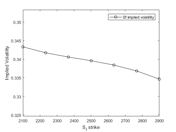
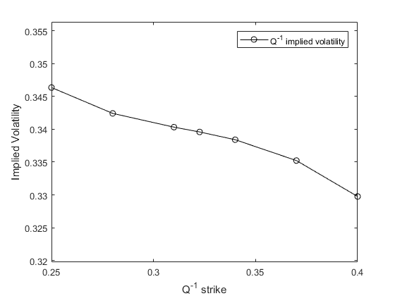
Figure 1: Implied volatilities for $S_{f}$ and $Q^{-1}$, as a function of strike, subject to a co-inclining volatility smile.

Both the DSW approach and the empirical copula approach adapt to the volatility smiles, while the practitioners’ approach does not, because of its “volatility is constant” assumption. Concerning the dependence relation between $S_{f}$ and $Q^{-1}$, the analysis is the same as in case I. Hence, no pricing differences should be observed between the DSW and the empirical copula frameworks (see Fig. 2). The minor differences observed between these two approaches are due to simulation imprecisions.

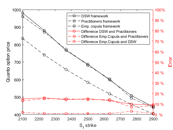
Figure 2: Pricing differences, Gaussian copula, co-inclining volatility smile.

4.3 Case III: $t$-student copula, long term option

In Cases III and IV, the matrix $\mathbb{A}$ is set such that the obtained copula is a $t$-copula with $3$ degrees of freedom and correlation $\rho(S_{f},Q^{-1})$,

$$\varphi_{S_{f}}=\varphi_{Q^{-1}}=(-0.7,1,0.1,0.2,0.5)$$

(whence a co-inclining volatility smile is obtained for $S_{f}$ and $Q^{-1}$, which is displayed in Figure 1). The time to maturity is $T=3$.

The practitioners’ framework is not capable of adapting to this case, because of the imposed volatility smile; and the DSW framework is not capable to adapt to this case either: while it is capable to adapt to the volatility smile, it is not able to adapt to the $t$-copula between $S_{f}$ and $Q^{-1}$. The latter presents more tail dependence than the Gaussian copula, which is intrinsic to the DSW framework. Hence, pricing differences are observed amongst all the three frameworks (see Figure 3). The slight difference between the DSW framework and our framework is attributed to the difference between a $t$-copula (with 3 degrees of freedom) and a Gaussian copula, with the same correlation parameter.

Figure 3: Pricing differences, $t$-student copula, long term option.

4.4 Case IV: $t$-student copula, short term option

In Case IV, the conditions are exactly the same as in Case III, except that $T=0.25$ instead of $T=3$.

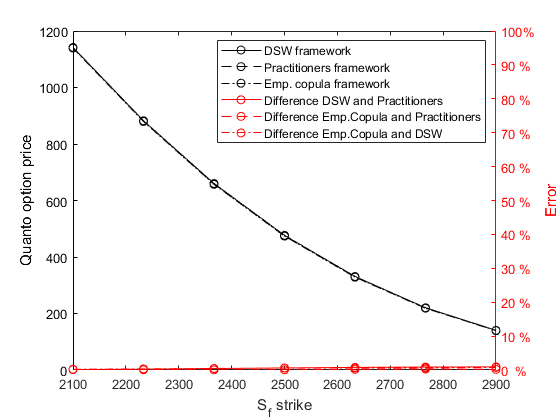
Figure 4: Pricing differences, $t$-student copula, short term option.

Figure 4 shows that no pricing differences are observed. We conclude that neither the dependence relation between $S_{f}$ and $Q^{-1}$ nor the volatility smile play a major role in the pricing of quanto options, if the contract is a short-term call option.

4.5 Case V: Frank copula, long term option

In this case, the same simple conditions as in Case $I$ are imposed, except that $\mathbb{A}$ is set such that the obtained copula is a Frank copula with parameter $\alpha$. The ordered pairs of quantiles generated by this copula, when converted to ordered pairs of normal random variables, induce a correlation $\rho(S_{f},Q^{-1})$. A Frank copula is less similar to a Gaussian copula than a $t$-copula is. Whence, this case stresses the modelling of the dependence relation more than Case $III$ does.

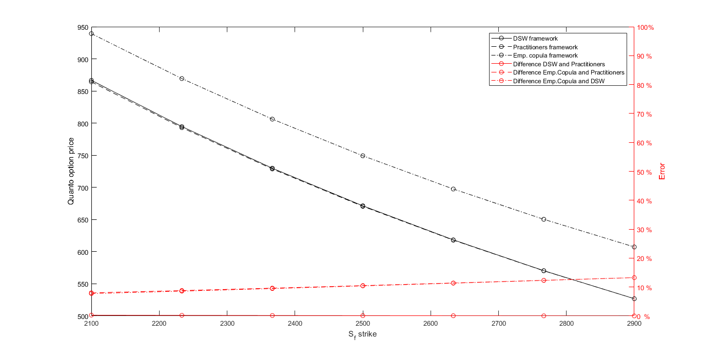
Figure 5: Pricing differences, Frank copula, long term option.

The DSW and the practitioners’ frameworks yield similar results, as no volatility smile is imposed and both approaches adapt to the imposed Frank copula dependence relation the same way, i.e., by considering solely its induced correlation. The empirical copula framework gives pricing figures considerably different from the other approaches as it takes into account the full dependence relation provided by the imposed Frank copula. Figure 5 illustrates these results.

4.6 Case VI: Frank copula, short term option

The conditions are the same as in Case V, except that now $T=0,25$. As a consequence, major pricing differences among the three models are not identified, even though slight pricing differences for deep out-of-the money options exist.

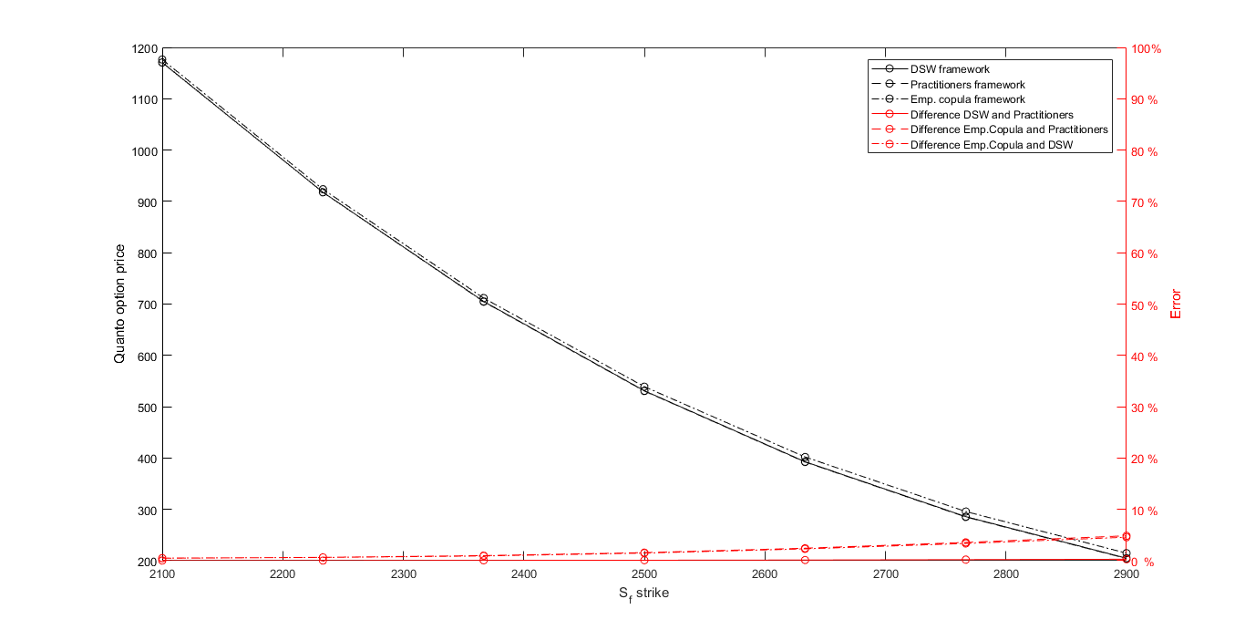
Figure 6: Pricing differences, Frank copula, short term option

Figure 6 illustrates the pricing differences. Whence, even in a stressed dependence relation context, the dependence relation does not play a major role in the pricing of short-term quanto options.

5 Summary

We have proposed a framework based on empirical copulas for quanto option pricing. We have given numerical examples in order to illustrate the pricing differences among our approach and the practitioners as well as the DSW model [1]. Looking at the results, we conclude that:

• the quanto option requires explicit modelling for accurate pricing, with the exception of short duration contracts;

• the flexibility provided by the empirical copula approach results in pricing differences when compared to the other two approaches.

On the proposed empirical copula dependence relation framework, we conclude that:

• it provides a flexible framework to define the dependence relation between the market variables used in quanto option pricing, by taking into account non-linear dependence relations, through the matrix $\mathbb{A}$ and the related empirical copula estimation framework;

• it can adapt to the observed volatility smiles from the relevant market variables, as the marginals of $S_{f}$ and $Q^{-1}$ shall be calibrated based on plain vanilla options market prices; and finally

• a drawback of the proposed model is that it is computationally more expensive than the other models it was compared to.

References

- [1] Dimitroff G., Szimayer A. and Wagner A., Quanto option pricing in the parsimonious Heston model, Berichte des Fraunhofer ITWM (2009) 1–24; Available at SSRN: http:// dx.doi.org/10.2139/ssrn.1477387.
- [2] Scaillet, O., and Fermanian, J.-D., Non-parametric estimation of copulas for time series (November 2002). FAME Research Paper No. 57. Available at SSRN: https://ssrn.com/abstract=372142 or http://dx.doi.org/10.2139/ssrn.372142.
- [3] Le Floc’h, F., On the simulation of a quanto process under local volatility (Sept. 2, 2011). Available at SSRN: https://ssrn.com/abstract=2097921; see also http://dx.doi.org/10.2139/ssrn.2097921.
- [4] Teng, L., Ehrhardt, M. and Günther, M., The pricing of quanto options under dynamic correlation, J. Computational and Applied Math. 275, February (2015) 304–310; https://doi.org/10.1016/j.cam.2014.07.017.r
- [5] Gramacki, A., Nonparametric Kernel Density Estimation and Its Computational Aspects, Springer 2018. Springer