Characterizing nonlocality of pure symmetric three-qubit states

Abstract

We explore nonlocality of three-qubit pure symmetric states shared between Alice, Bob and Charlie using the Clauser-Horne-Shimony-Holt (CHSH) inequality. We make use of the elegant parametrization in the canonical form of these states, proposed by Meill and Meyer (Phys. Rev. A 96, 062310 (2017)) based on Majorana geometric representation. The reduced two-qubit states, extracted from an arbitrary pure entangled symmetric three-qubit state do not violate the CHSH inequality and hence they are CHSH-local. However, when Alice and Bob perform a CHSH test, after conditioning over measurement results of Charlie, nonlocality of the state is revealed. We have also shown that two different families of three-qubit pure symmetric states, consisting of two and three distinct spinors (qubits) respectively, can be distinguished based on the strength of violation in the conditional CHSH nonlocality test. Furthermore, we identify six of the 46 classes of tight Bell inequalities in the three-party, two-setting, two-outcome i.e., (3,2,2) scenario (Phys. Rev. A 94, 062121 (2016)). Among the two inequivalent families of three-qubit pure symmetric states, only the states belonging to three distinct spinor class show maximum violations of these six tight Bell inequalities.

1 Introduction

Correlations arising from local measurements made on a spatially separated composite quantum system are nonlocal if the underlying measurement statistics cannot be reproduced using classical strategies. Violation of Bell inequalities bell1 ; chsh certifies the presence of nonlocality. There has been a growing demand for more general ways of characterizing nonlocality and over the years different theoretical formulations of Bell inequalities have been proposed cavalcanti ; rchaves ; rmp ; lewenstein1 ; lewenstein2 to capture nonlocality exhibited by shared multipartite quantum states. Composite quantum states which violate Bell inequality are necessarily entangled but the converse is not necessarily true. Characterization of entanglement and nonlocality of multipartite quantum systems has gained growing importance as they play a key role in several quantum information processing tasks rmp .

Multiqubit states which respect exchange symmetry form an important class of composite quantum systems. Examples of these states are the well known GHZ and W states aditimark ; bastin ; aru . Permutation symmetric multiqubit states have attracted much attention in view of their applications in quantum information processing. Entanglement properties of symmetric multiqubit states have been studied extensively aditimark ; bastin ; markham ; aru ; toth ; aru1 ; aru2 ; aru3 . Confining to the special class of permutation symmetric states leads to reduction in the number of parameters and this in turn helps in simplifying evaluations in an explicit manner. Moreover, nonlocality of multiqubit states obeying exchange symmetry have been investigated using experimentalist-friendly Bell inequalities involving multiqubit observables exhibiting one and two qubit correlations only lewenstein1 ; lewenstein2 .

Recently Meill and Meyer meyer employed a canonical form for permutation symmetric pure entangled three-qubit states based on the Majorana geometric representation bastin ; aru ; majorana and evaluated the algebraically independent local unitary invariant quantities. Majorana geometric representation offers a natural classification of entangled pure symmetric three-qubit states, consisting of two and three distinct spinors (qubits), which can be represented by distinct points on the Bloch sphere. This structure leads to an elegant parametrization for the entangled pure symmetric three-qubit states meyer and facilitates explicit evaluation of local unitary invariants viz., the pairwise concurrence $C$, the three-tangle $\tau$ and the Kempe invariant $\kappa$. It would be interesting to explore nonlocality features of the entire family of entangled pure permutation symmetric three-qubit states using their canonical structure – equipped with a neat parametrization, resulting from the Majorana geometric representation. We focus here on investigating nonlocality of entangled pure symmetric three-qubit states using conditional CHSH inequality cavalcanti ; rchaves and the tight Bell inequalities of the (3,2,2) scenario (i.e., Bell tests in the three-party, two-setting, two-outcome scenario) pit01 ; silwa ; cab1 ; cab2 .

We begin by verifying that the reduced two-qubit density matrices – extracted from the entangled pure symmetric three-qubit states – are CHSH-local. It is pertinent to recall here that Popescu and Rohrlich had shown PR that a bipartite system prepared by carrying out projective measurements on the $N-2$ parties of any pure entangled $N$-party state is nonlocal. This prompts us to study violation of the conditional CHSH inequality cavalcanti ; rchaves by two-qubit states obtained after an outcome of a projective measurement on the third qubit is recorded. This provides a succinct illustration that non locality of the reduced two-qubit state indeed gets activated by conditioning over the outcomes of measurement made on the third qubit, thereby offering a preview of the nonlocality content of the global pure entangled symmetric three-qubit state. We show that the optimal violation of conditional CHSH inequality is different for the classes of entangled pure symmetric three-qubit states, consisting of two and three distinct spinors respectively. Furthermore, we show that six of the 46 classes of tight Bell inequalities in the (3,2,2) scenario get violated maximally by pure symmetric three-qubit states belonging to the three distinct spinor Majorana class.

This paper is organized as follows: Section 2 gives a brief introduction of the Majorana geometric representation bastin ; aru ; meyer ; majorana of pure entangled three-qubit symmetric states and their classification under stochastic local operations and classical communications (SLOCC) into two different classes. We employ the parametrization given in Ref. meyer to characterize these two SLOCC inequivalent classes. In Section 3, optimal expectation values of the Bell-CHSH operator are explicitly evaluated (in terms of the eigenvalues of the two-qubit correlation matrices horodecki95 ) for the SLOCC inequivalent classes of pure symmetric three-qubit states. It is demonstrated that the CHSH inequality is not violated by any pairs of qubits extracted from an entangled pure three-qubit symmetric state. In Section 4, violation of conditional CHSH inequality by the states under consideration is illustrated. Bell inequalities of the (3,2,2) scenario are discussed in Section 5 and a concise summary of our results is given in Section 6.

2 Three-qubit pure symmetric states: SLOCC inequivalent classes

An arbitrary pure symmetric three-qubit state can be expressed in the Majorana geometric representation bastin ; aru ; majorana by

$$|\Psi_{\rm sym}\rangle = {\cal N}\sum_{P}\hat{P}\{|\alpha_{1},\beta_{1}\,\rangle\otimes|\alpha_{2},\beta_{2}\rangle\otimes|\alpha_{3},\beta_{3}\rangle\}$$ (1)

where,

$$|\alpha_{k},\beta_{k}\rangle\equiv\cos\frac{\beta_{k}}{2}\,|0\rangle+e^{i\alpha_{k}}\,\sin\frac{\beta_{k}}{2}\,|1\rangle,\ \ k=1,\,2,\,3,$$ (2)

denote qubit states where $0\leq\alpha_{k}\leq 2\pi,$ $0\leq\beta_{k}\leq\pi$. Here $\hat{P}$ corresponds to the set of all permutations on the constituent qubits and ${\cal N}$ denotes the normalization factor.

Depending on the number of distinct spinor states $\{|\alpha_{k},\beta_{k}\,\rangle,\,k=1,2,3\}$ there arise two different classes of entangled pure symmetric states of three qubits aru :

1. Two distinct spinor class: $|\alpha_{1},\beta_{1}\rangle=|\alpha_{2},\beta_{2}\rangle\neq|\alpha_{3},\beta_{3}\rangle$

2. Three distinct spinor class: $|\alpha_{1},\beta_{1}\rangle\neq|\alpha_{2},\beta_{2}\rangle\neq|\alpha_{3},\beta_{3}\rangle$.

It may be noted that when the constituent qubit states are all identically equal i.e., $|\alpha_{1},\beta_{1}\rangle=|\alpha_{2},\beta_{2}\rangle=|\alpha_{3},\beta_{3}\rangle=|\alpha,\beta\rangle$ the pure state $|\Psi_{\rm sym}\rangle$ reduces to a separable (product) form $|\,\alpha,\beta\rangle^{\otimes\,3}$.

Let us denote the two distinct spinor class of pure three-qubit states by $\{{\cal{D}}_{3,2}\}$ and the three distinct spinor class by $\{{\cal{D}}_{3,3}\}$. These two classes are evidently inequivalent under SLOCC aru . Examples of three-qubit states of the class $\{{\cal{D}}_{3,2}\}$ are

$$|{\rm W}\rangle = {\cal N}\,\sum_{P}\hat{P}\{|0\,\rangle\otimes|0\,\rangle\otimes|1\,\rangle\}$$ (3)

$$= \frac{1}{\sqrt{3}}\,\left(|0\,0\,1\rangle+|0\,1\,0\rangle+|1\,0\,0\rangle\right)$$

and its obverse state $|\bar{{\rm W}}\rangle=\frac{1}{\sqrt{3}}\,\left(|1\,1\,0\rangle+|1\,0\,1\rangle+|0\,1\,1\rangle\right)$. A paradigmatic example of the three-qubit symmetric state belonging to the SLOCC class $\{{\cal{D}}_{3,3}\}$ is the GHZ state GHZ :

$$|{\rm GHZ}\rangle = {\cal N}\,\sum_{P}\hat{P}\{|\,\phi\rangle_{1}\,\otimes|\,\phi\rangle_{2}\otimes|\phi\rangle_{3}\}$$ (4)

$$= \frac{1}{\sqrt{2}}\,\left(|0\,0\,0\rangle+|1\,1\,1\rangle\right)$$

where $|\phi\rangle_{p}=\frac{1}{\sqrt{2}}(|0\rangle+\omega^{p}\,|1\rangle),p=1,2,3$ are the constituent qubit states and $\omega$ denotes cube root of unity. Another illustrated example of three-qubit state belonging to the class $\{{\cal{D}}_{3,3}\}$ is the superposition of $|{\rm W}\rangle$ and $|\bar{{\rm W}}\rangle$ states aditimark ; aru :

$$|{\rm W}\,\bar{{\rm W}}\rangle = {\cal N}\,\sum_{P}\hat{P}\{|0\,\rangle\otimes|1\,\rangle\otimes|+\rangle\}$$ (5)

where $|+\rangle=\frac{1}{\sqrt{2}}(|0\rangle+|1\rangle)$.

It has been shown that any arbitrary three-qubit pure state of two distinct spinor class $\{{\cal{D}}_{3,2}\}$ takes the following simple form with the help of local unitary operations meyer :

$$|\Psi_{3,\,2}\rangle = {\cal N}\sum_{P}\hat{P}\{|0\rangle\otimes|0\rangle\otimes|\beta\rangle\}$$ (6)

where

$$|\beta\rangle=\cos\,\frac{\beta}{2}\,|0\rangle+\sin\,\frac{\beta}{2}\,|1\rangle$$ (7)

Thus the states belonging to the class $\{{\cal{D}}_{3,2}\}$ are characterized by one real parameter specified by $0<\beta\leq\pi$. Note that the state $|\Psi_{3,\,2}\rangle$ reduces to the three-qubit $W$ state when $\beta=\pi$.

An arbitrary three-qubit pure symmetric state belonging to the class $\{{\cal{D}}_{3,3}\}$ of three distinct spinor is shown meyer to be characterized by three real parameters:

$$|\Psi_{3,3}\rangle = {\cal N}\left(|0\,\rangle^{\otimes\,3}+y\,e^{i\,\alpha}\,|\beta\rangle^{\otimes\,3}\right)$$ (8)

where the qubit state $|\beta\rangle$ is given by (7); the real parameters $y$ and $\alpha$ are bounded by $0<y\leq 1,\ 0\leq\alpha\leq 2\pi$. We make use of this explicit parametrization of three-qubit symmetric states for exploring their nonlocality.

3 Bell-CHSH nonlocality test

Consider the reduced two-qubit density matrix of a pure symmetric three-qubit state $|\Psi\rangle_{\rm sym}$ shared by Alice, Bob and Charlie:

$$\rho_{\rm R} = {\rm Tr}_{A}\,\left(|\Psi\rangle_{\rm sym}\langle\Psi|\right)={\rm Tr}_{B}\,\left(|\Psi\rangle_{\rm sym}\langle\Psi|\right)$$

$$= {\rm Tr}_{C}\,\left(|\Psi\rangle_{\rm sym}\langle\Psi|\right)$$

In the Hilbert-Schmidt basis we express

$$\rho_{\rm R} = \frac{1}{4}\left[I\otimes I+\sum_{i=1}^{3}\,s_{i}\left(\sigma_{i}\otimes I+I\otimes\sigma_{i}\right)\right.$$ (9)

$$\left.+\sum_{i,j=1}^{3}\,t_{ij}\,(\sigma_{i}\otimes\sigma_{j})\right]$$

where $\sigma_{i}$, $i=1,\,2,\,3$ are the Pauli matrices; $I$ denotes $2\times 2$ identity matrix and the real parameters $s_{i}$, $t_{ij}$ are given by

$$s_{i} = {\rm Tr}\left[\rho_{R}\,(\sigma_{i}\otimes I)\right]={\rm Tr}\left[\rho_{R}\,(I\otimes\sigma_{i})\right]$$

$$t_{ij} = {\rm Tr}\left[\rho_{R}\,(\sigma_{i}\otimes\sigma_{j})\right]=t_{ji}.$$ (10)

The correlation matrix $T=(t_{ij})$ of the permutation symmetric density matrix $\rho_{R}$ is a $3\times 3$ real symmetric matrix satisfying the condition aru1 ; aru2 ${\rm Tr}(T)=1$.

We consider the CHSH inequality chsh given by

$$\langle{\rm CHSH}\rangle=|\langle A_{1}\,B_{1}+A_{1}\,B_{2}+A_{2}\,B_{1}-A_{2}\,B_{2}\rangle|\leq 2$$ (11)

where

$$\langle A_{i}\,B_{j}\rangle=\sum_{a_{i},b_{j}=\pm 1}\,a_{i}\,b_{j}\ p(a_{i},b_{j}|A_{i},B_{j}),\ \ i,\,j=1,\,2.$$ (12)

Here $p(a_{i},\,b_{j}|A_{i},B_{j})$, $i,\,j=1,2$, denote the correlation probabilities evaluated based on the outcomes $a_{i}$, $b_{j}$ of the observables $A_{i}$, $B_{j}$ of Alice and Bob respectively.

Maximum value $\langle{\rm CHSH}\rangle_{\rm opt}$ achievable by any arbitrary two-qubit state is given by horodecki95

$$\langle{\rm CHSH}\rangle_{\rm opt}=2\sqrt{t_{1}^{2}+t_{2}^{2}}$$ (13)

where $t_{1}^{2}$, $t_{2}^{2}$ denote two largest eigenvalues of $T^{\dagger}\,T$.

The parametrization (6), (8) of the pure three-qubit symmetric states facilitates evaluation of the correlation matrix $T$ of the reduced two-qubit state $\rho_{R}$ belonging to the SLOCC inequivalent classes $\{{\cal D}_{3,2}\}$, $\{{\cal D}_{3,3}\}$. Utilizing this structure one may compute the optimal CHSH value to test nonlocality. We carry out such an analysis in the following subsections.

3.1 Bell-CHSH test on the two-qubit states of the SLOCC class $\{{\cal D}_{3,2}\}$

We evaluate the correlation matrix $T$ (see (10)) of the two-qubit reduced density matrix $\rho_{R}$ associated with the one-parameter family (6) of pure symmetric states belonging to the SLOCC class $\{{\cal D}_{3,\,2}\}$ explicitly:

$$T=\frac{1}{3(2+\cos\beta)}\left(\begin{array}[]{cccc}1-\cos\beta&0&3\sin\beta\\ 0&1-\cos\beta&0\\ 3\sin\beta&0&4+5\cos\beta\end{array}\right)$$ (14)

and obtain its eigenvalues 

$$t_{1} = \frac{5+4\cos\beta+3\sqrt{5+4\cos\beta}}{6(2+\cos\beta)}$$

$$t_{2} = \frac{1-\cos\beta}{3(2+\cos\beta)}$$ (15)

$$t_{3} = \frac{5+4\cos\beta-3\sqrt{5+4\cos\beta}}{6(2+\cos\beta)}.$$

We have plotted the absolute values of $t_{1},t_{2}$ and $t_{3}$ in Figure 1 from which it is readily seen that $|t_{1}|\geq|t_{2}|\geq|t_{3}|$.

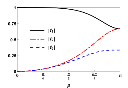
Figure 1: (Color online) Absolute values of $t_{1}$ (black,solid), $t_{2}$ (red, dot-dashed) and $t_{3}$ (blue, dashed) (see (3.1)) as a function of the parameter $\beta$

.

Figure 2: Optimal value $\langle{\rm CHSH}\rangle_{\rm opt}$ achievable in the two-qubit reduced state, associated with the class $\{{\cal{D}}_{3,2}\}$ of entangled pure symmetric three-qubit states, as a function of $\beta$.

Figure 2 depicts a plot of $\langle{\rm CHSH}\rangle_{\rm opt}$ (See (13)) as a function of $\beta$. Evidently, $\langle{\rm CHSH}\rangle_{\rm opt}\leq 2$ in the entire range of the parameter $\beta$. This leads to an explicit verification of the result that reduced two-qubit states of entangled pure symmetric three-qubit states belonging to the class $\{{\cal{D}}_{3,2}\}$ are CHSH-local.

3.2 Bell-CHSH test on the two qubit states of $\{{\cal D}_{3,3}\}$

We now proceed to study the Bell-CHSH nonlocality exhibited by a pair of qubits extracted from the three-qubit states belonging to the SLOCC class $\{{\cal D}_{3,3}\}$. Towards this end, we proceed to evaluate the eigenvalues $|t_{1}|\geq|t_{2}|\geq|t_{3}|$ of the correlation matrix $T$ (see (10)) so as to compute the optimal CHSH value $\langle{\rm CHSH}\rangle_{\rm opt}=2\sqrt{t_{1}^{2}+t_{2}^{2}}$.

The state $|\Psi_{3,\,3}\rangle\in\{{\cal D}_{3,3}\}$ (see (8)) is characterized by three real independent parameters: $0<\beta\leq\pi$, $0<y\leq 1$, $0\leq\alpha\leq 2\pi$. We have verified numerically that the two-qubit states $\rho_{R}$ extracted from $|\Psi_{3,\,3}\rangle\in\{{\cal D}_{3,3}\}$ are all local. We choose two specific sets of parameters $(y,\alpha,\beta)$ for the purpose of explicit demonstration.

Listed below are two specific choices of parameters $(\alpha,\beta)$ and two largest eigen values $t_{1},t_{2}$ of the correlation matrix $T$ of the associated reduced two-qubit states:

• $\beta=\pi/2$, $\alpha=\pi$

  $$t_{1} = \frac{1-\sqrt{2}y+y^{2}+\sqrt{1+y^{4}}}{2-\sqrt{2}y+2y^{2}},$$

  $$t_{2} = \frac{y}{\sqrt{2}(1+y^{2})-y}$$ (16)

• $\beta=\pi/3$, $\alpha=0$

  $$t_{1,\,2}=\frac{2(1+\sqrt{3}y+y^{2}\pm\sqrt{1+\sqrt{3}y+2y^{2}+\sqrt{3}y^{3}+y^{4}})}{4+3\sqrt{3}y+4y^{2}}$$ (17)

We have plotted $\langle{\rm CHSH}\rangle_{\rm opt}=2\,\sqrt{t_{1}^{2}+t_{2}^{2}}$ as a function of the state parameter $y$ in the cases (i) $\beta=\pi/2$, $\alpha=\pi$ and (ii) $\beta=\pi/3$, $\alpha=0$ in Figure 3.

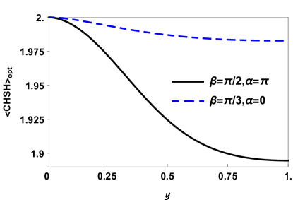
Figure 3: (Color online) Optimal CHSH value $\langle{\rm CHSH}\rangle_{\rm opt}$ that can be realized in the two-qubit reduced state of $|\Psi_{3,3}\rangle$ (see (8)) belonging to the three distinct spinor class $\{{\cal{D}}_{3,3}\}$ as a function of the parameter $y$ for specific cases of parameters (i) $\beta=\pi/2,\,\alpha=\pi$ (black, solid) and (ii) $\beta=\pi/3,\,\alpha=0$ (blue, dashed)

This demonstrates that the maximum CHSH value $\langle{\rm CHSH}\rangle_{\rm opt}$ evaluated in a reduced two-qubit state drawn from three-qubit states $|\Psi_{3,3}\rangle$ (see (8)) of the three distinct spinor class $\{{\cal{D}}_{3,3}\}$ is less than or equal to 2 and thus the state is local.

4 Conditional CHSH test

In Ref. PR Popescu and Rohrlich considered a generalized CHSH inequaltiy involving correlations between two systems, conditioned on a particular measurement outcome registered by the $N-2$ systems. They proved that any bipartite system prepared by carrying out an optimal projective measurements on the $N-2$ parties of any pure entangled $N$-party state violated the conditional CHSH inequality. More recently, the CHSH violation of two out of the $N$ qubits conditioned on a measurement outcome of all other $N-2$ qubits has been employed cavalcanti ; rchaves to certify the nonlocality of multipartite quantum states. In this section we investigate the violation of the conditional CHSH inequality by entangled pure symmetric three-qubit states.

Let us consider an entangled pure symmetric three-qubit state, shared by Alice, Bob and Charlie. Charlie performs a projective measurement $P_{c}$ on his qubit, which yields a particular outcome $c=\pm 1$ (with probability $p(c)$). Conditioned on Charlie’s outcome, Alice and Bob perform local measurements (two settings each) of the observables $A_{i},\,B_{j},\,i,j=1,2$ on their respective qubits and get dichotomic outcomes $a_{i},b_{j}=\pm 1$. The conditional CHSH inequality is given by cavalcanti ; rchaves

$$\left|\langle\,A_{1}\,B_{1}\rangle_{c}+\langle\,A_{1}\,B_{2}\rangle_{c}+\langle\,A_{2}\,B_{1}\rangle_{c}-\langle\,A_{2}\,B_{2}\rangle_{c}\right|\leq 2\,p(c)$$ (18)

where

$$\langle A_{i}\,B_{j}\rangle_{c}=p(c)\,\sum_{a_{i},b_{j}=\pm 1}\,a_{i}\,b_{j}\,p(a_{i},b_{j}|A_{i},B_{j},c).$$ (19)

Summation over $c=\pm 1$ leads to the following inequality (see Eq. (14) of Ref.rchaves ):

$$\sum_{c=\pm 1}\,\left|\langle\,A_{1}\,B_{1}\rangle_{c}+\langle\,A_{1}\,B_{2}\rangle_{c}+\langle\,A_{2}\,B_{1}\rangle_{c}-\langle\,A_{2}\,B_{2}\rangle_{c}\right|\leq 2\,$$ (20)

In a given pure entangled three qubit symmetric state $|\Psi_{\rm sym}\rangle$, Charlie chooses a suitable local measurement $P_{c}$ and performs a projective measurement on his qubit to obtain a particular outcome $c=\pm 1$. Charlie’s measurement, in turn, projects the two-qubit state of Alice & Bob such that the conditional CHSH inequality given by (20) gets violated. Such violation clearly demonstrates activation of hidden-nonlocality gisin .

In order to verify optimal violation of the conditional CHSH inequalities (18) and (20) we need to compute two largest eigenvalues $t_{1}^{c},t_{2}^{c}$ of the two-qubit conditional correlation matrix $T^{c},\,c=\pm 1,$ so that

$$\langle{\rm CHSH}\rangle_{c,\rm opt} = 2\,\sqrt{(t^{c}_{1})^{2}+(t^{c}_{2})^{2}}>2$$ (21)

$$\langle{\rm CHSH}\rangle^{\rm con}_{\rm opt} = 2\,\sum_{c=\pm 1}\,p(c)\,\langle{\rm CHSH}\rangle_{c,\rm opt}$$ (22)

$$= 2\,\sum_{c=\pm 1}\,p(c)\,\sqrt{(t^{c}_{1})^{2}+(t^{c}_{2})^{2}}>2$$

where

$$p(c)=\langle\Psi_{\rm sym}|\,(I\otimes I\otimes P_{c})\,|\Psi_{\rm sym}\rangle$$ (23)

denotes probability of obtaining the outcome $c=\pm 1$ by Charlie for his local projective measurement $P_{c}$.

Note that the matrix elements $t^{c}_{ij}$ of the two-qubit correlation matrix $T^{c}$ are given by

$$t^{c}_{ij}=\langle\Psi_{\rm sym}|\sigma_{i}\otimes\sigma_{j}\otimes P_{c}\,|\Psi_{\rm sym}\rangle,\ \ i,j=1,2,3.$$ (24)

We denote Charlie’s projective measurement by

$$P_{c}(\theta,\phi) = \frac{1}{2}\,\left(I+c\ \vec{\sigma}\cdot\hat{n}(\theta,\phi)\,\right),$$ (25)

where $\hat{n}(\theta,\phi)~{}=~{}(\sin\,\theta\cos\,\phi,\,\sin\,\theta\sin\,\phi,\,\cos\,\theta)$, $0~{}\leq~{}\theta~{}\leq~{}\pi,\ \ 0~{}\leq~{}\phi~{}\leq~{}2\pi$ denotes a unit vector corresponding to the measurement setting of Charlie.

4.1 Violation of the conditional CHSH inequality by states of the SLOCC class $\{{\cal{D}}_{3,2}\}$

We proceed to compute optimal conditional CHSH values $\langle{\rm CHSH}\rangle_{c,{\rm opt}},\,\langle{\rm CHSH}\rangle^{\rm con}_{\rm opt}$ (see (21),(22)) in the one parameter family of states $|\Psi_{3,2}\rangle$ given by (6) which belong to the two distinct spinor SLOCC class $\{{\cal{D}}_{3,2}\}$.

On explicit evaluation, elements of the conditional correlation matrix $T^{c}$ (See (24)) corresponding to states $|\Psi_{3,2}\rangle$ are obtained as

$$t^{c}_{11} = \left[(1+c\,\cos\theta)(1-\cos\beta)\right]/\mu_{c}=t^{c}_{22}\$$

$$t^{c}_{12} = t^{c}_{21}=0$$

$$t^{c}_{13} = \left[3(1+c\cos\theta)\sin\beta+c\,\cos\phi\sin\theta(1-\cos\beta)\right]/\mu_{c}=t^{c}_{31}$$

$$t^{c}_{23} = \left[c\,\sin\theta\,\sin\phi\,(1-\cos\beta)\right]/\mu_{c}=t^{c}_{32},\ \$$

$$t^{c}_{33} = 1-2\,t^{c}_{11}$$ (26)

where we have denoted

$$\mu_{c} = 6+5\,c\,\cos\theta+(3+4\,c\,\cos\theta)\,\cos\beta+3\,c\,\cos\phi\,\sin\beta\,\sin\theta.$$ (27)

Substituting (25) and (6) in (23) we obtain Charlie’s probability of getting the measurement outcome $c=\pm 1$ in the state $|\Psi_{3,2}\rangle$:

$$p(c)=\frac{\mu_{c}}{6(2+\cos\beta)}$$ (28)

Eigenvalues of the correlation matrix $T^{c}$ are given by

$$t^{c}_{1}=1,\ t^{c}_{2}=\frac{(1+c\cos\theta)(1-\,\cos\beta)}{\mu_{c}}=-t^{c}_{3}$$ (29)

Figure 4: (Colour online) Slice contour plots of the optimal value $\langle{\rm CHSH}\rangle_{c=1,{\rm opt}}$ as a function of the state parameter $\beta$ and Charlie’s projective measurement orientation angles $(\theta,\,\phi)$ evaluated in the state $|\Psi_{3,2}\rangle$ [see (6)] of the SLOCC class $\{{\cal{D}}_{3,2}\}$. It is evident that the inequality (18) gets violated in the entire parameter range $0<\beta\leq\pi$ in the state $|\Psi_{3,2}\rangle\in\{{\cal{D}}_{3,2}\}$, when a conditioning over Charlie’s measurement outcomes is done. It is also seen that $\langle{\rm CHSH}\rangle_{c=1,{\rm opt}}$ approaches the allowed maximal value of $2\sqrt{2}$ for a specific range of values of the state parameter $\beta$ and for the orientations $(\theta,\phi)$ of Charlie’s measurement.

In Figure 4 we have presented a slice contour plot of the optimal value $\langle{\rm CHSH}\rangle_{c=1,{\rm opt}}=2\,\sqrt{(t^{c=1}_{1})^{2}+(t^{c=1}_{2})^{2}}$ evaluated in the two distinct spinor states $|\Psi_{3,2}\rangle$ given by (6) as a function of the state parameter $\beta$ and Charlie’s measurement settings $\theta$, $\phi$. It is evident that the one parameter family of states $|\Psi_{3,2}\rangle\in\{{\cal{D}}_{3,2}\}$ violate the conditional CHSH inequality (18) in the entire range of the parameter $0<\beta\leq\pi$. In particular, by conditioning on Charlie’s measurement outcome $c=1$ in the $|{\rm W}\rangle$ state, obtained by substituting $\beta=\pi$ in $|\Psi_{3,2}\rangle$ (see (3) and (6)), it is possible to witness maximum violation $\langle{\rm CHSH}\rangle_{c=1,{\rm opt}}=2\sqrt{2}\approx 2.828$.

A plot of the optimal value $\langle{\rm CHSH}\rangle^{\rm con}_{\rm opt}=2\,\sum_{c=\pm 1}\,p(c)\,\sqrt{(t^{c}_{1})^{2}+(t^{c}_{2})^{2}}$, as a function of the state parameter $\beta$ and Charlie’s projective measurement settings $\theta$, $\phi$ is given in Figure 5. It is seen that the maximum value of $\langle{\rm CHSH}\rangle^{\rm con}_{\rm opt}$ in the one-parameter family of states $|\Psi_{3,2}\rangle$ belonging to the SLOCC class $\{{\cal{D}}_{3,2}\}$ can atmost be equal to 2.55 and does not attain the largest possible value $2\sqrt{2}\approx 2.828$.

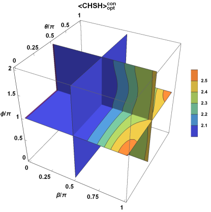
Figure 5: (Colour online) Slice contour plot of the optimal value $\langle{\rm CHSH}\rangle^{\rm con}_{\rm opt}$ in the one parameter family of states $|\Psi_{3,2}\rangle$ (see (6)) of the SLOCC class $\{{\cal{D}}_{3,2}\}$ as a function of the state parameter $\beta$ and Charlie’s measurement orientation angles $\theta$, $\phi$. Note that the largest value $\langle{\rm CHSH}\rangle^{\rm con}_{\rm opt}$ achievable in the one-parameter family of states $|\Psi_{3,2}\rangle$ belonging to the SLOCC class $\{{\cal{D}}_{3,2}\}$ is  2.55.

4.2 Conditional CHSH nonlocality test on the SLOCC class $\{{\cal{D}}_{3,3}\}$

We continue to carry out conditional CHSH nonlocality test on the states $|\Psi_{3,3}\rangle$ belonging to the three distinct spinor SLOCC class $\{{\cal{D}}_{3,3}\}$. The states defined in (8) are characterized by three real parameters. The conditional correlation matrix $T^{c}$ depends on the state parameters $y,\alpha,\,\beta\,$ and Charlie’s measurement orientations $\theta,\phi$. For the sake of illustration we fix $y=1$, $\alpha=0$. With this choice of parameters the following eigenvalues $t^{c}_{1},\,t^{c}_{2},t^{c}_{3}$ of the conditional correlation matrix $T^{c}$ are obtained:

$$t^{c}_{1} = 1,$$

$$t^{c}_{2} = \frac{1}{\nu_{c}}\,\left[2\,\left(1+c\,\cos\theta\right)\,\left(1-\,\cos\beta\right)^{3}\,\left(1+c\,\cos\theta\,\cos\beta+c\,\cos\phi\,\sin\theta\,\sin\beta\right)\right]^{1/2}\,$$ (30)

$$= \,-t^{c}_{3},$$

where

$$\nu_{c} = \cos\phi\sin\theta\sin\beta\,(1+\sin\beta)+2\sin\left(\frac{\beta}{2}\right)\left[2\,c\left(1+\cos^{3}\left(\frac{\beta}{2}\right)\right)\right.$$ (31)

$$\left.+\cos\theta\left(1+2\cos^{3}\left(\frac{\beta}{2}\right)+\cos\beta\right)\right].$$

Probability of the measurement outcome $c=\pm 1$ when Charlie performs projective measurement $P_{c}(\theta,\phi)$ (see (25)) on his qubit is given by

$$p(c) = \frac{2+c\,\cos\theta(1+\cos\beta)}{4\,\left[1+\cos^{3}\left(\frac{\beta}{2}\right)\right]}$$

$$+ \frac{2\,\cos^{3}\left(\frac{\beta}{2}\right)(1+c\,\cos\theta)+c\,\cos\phi\,\sin\theta\,\sin\beta\,\left(1+\cos\left(\frac{\beta}{2}\right)\right)}{4\,\left[1+\cos^{3}\left(\frac{\beta}{2}\right)\right]}$$

In Figure 6 we present plots of the optimal values $\langle{\rm CHSH}\rangle_{c=1,{\rm opt}}=2\sqrt{(t^{c}_{1})^{2}+(t^{c}_{2})^{2}}$, evaluated in the entangled pure symmetric three-qubit state $|\Psi_{3,3}\rangle$ (see (8)) as a function of Charlie’s projective measurement orientations $(\theta,\,\phi)$ and one of the state parameters $0<\beta\leq\pi$ – for the specific choices $y=1,\,\alpha=0$. (The parameters $y$ and $\alpha$ are chosen in order to witness largest possible violation in this SLOCC class of states).

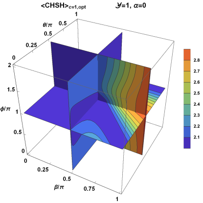
Figure 6: (Colour online) Slice contour plot of $\langle{\rm CHSH}\rangle_{c=1,{\rm opt}}~{}=~{}2\sqrt{(t^{c=1}_{1})^{2}+(t^{c=1}_{2})^{2}}$ for $c=1$, in the state $|\Psi_{3,3}\rangle$ (see (8)) of the SLOCC class $\{{\cal{D}}_{3,3}\}$ as a function of one of the state parameter $\beta$ and Charlie’s projective measurement settings $\theta$, $\phi$. Here we have fixed the values $y=1,\,\alpha=0$ of the other two parameters characterizing the state. It is seen that the conditional CHSH inequality (18) gets violated upto the allowed maximum value $2\sqrt{2}$ for some specific values of the parameter $\beta$ and Charlie’s measurement orientations $\theta$, $\phi$.

It can be seen that for some specific values of $\beta,\theta$ and $\phi$, $\langle{\rm CHSH}\rangle_{c=1,{\rm max}}=2\sqrt{2}$ implying maximum violation of conditional CHSH inequality (18). In particular, GHZ state (obtained by substituting $\beta=\pi$ in $|\Psi_{3,3}\rangle$ of (8)) violates (18) (as well as (20)) maximally.

We also present contour plot of the optimal conditional CHSH value (see (22))

$$\langle{\rm CHSH}\rangle^{\rm con}_{\rm opt}=2\,\sum_{c=\pm 1}\,p(c)\,\sqrt{(t^{c}_{1})^{2}+(t^{c}_{2})^{2}}$$

in Figure 7. It is seen that there exist three qubit states belonging to the three distinct spinor SLOCC class $\{{\cal{D}}_{3,3}\}$ which violate the conditional CHSH inequality (20) all the way up to the maximum possible value $2\sqrt{2}$.

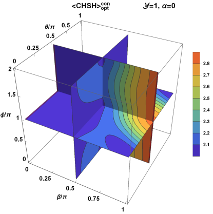
Figure 7: (Colour online) Slice contour plot of $\langle{\rm CHSH}\rangle^{\rm con}_{\rm opt}$ in the three parameter family of states $|\Psi_{3,3}\rangle$ (see (8)) of the three distinct spinor SLOCC class $\{{\cal{D}}_{3,3}\}$, as a function of one of the state parameters $\beta$ and Charlie’s measurement direction $\theta$ and $\phi$ – for the specific choice $y=1$, $\alpha=0$. It is clearly seen that the conditional CHSH value $\langle{\rm CHSH}\rangle^{\rm con}_{\rm opt}$ approaches its allowed maximum value $2\sqrt{2}\approx 2.828$ for specific range of the state parameter $\beta$ and Chalie’s measurement orientations $\theta,\,\phi$.

While we have seen from Figure 5 that the maximal value of $\langle{\rm CHSH}\rangle^{\rm con}_{\rm opt}$ achieved in the one parameter family of states $|\Psi_{3,\,2}\rangle$ belonging to the two distinct spinor SLOCC class $\{{\cal D}_{3,2}\}$ is $~{}2.55$, from Figure 7 it is evident that the largest value of $\langle{\rm CHSH}\rangle^{\rm con}_{\rm opt}$ for the states $|\Psi_{3,\,3}\rangle$ of the class $\{{\cal D}_{3,3}\}$ goes up to the largest possible value $2\sqrt{2}$. This prompts us to quantify the nonlocality of entangled three-qubit symmetric states by defining the quantity ${\cal Q}$

$${\cal Q}={\rm max}\left\{0,\,\frac{\langle{\rm CHSH}\rangle^{\rm con}_{\rm opt}-2}{2\sqrt{2}-2}\right\}$$ (32)

which increases from 0 to 1 as $\langle{\rm CHSH}\rangle^{\rm con}_{\rm opt}$ changes from $2$ to $2\sqrt{2}.$ Based on numerical evaluations it is found that the nonlocality quantifier ${\cal Q}$ does not vanish in the entire range of parameters of the three-qubit states $|\Psi_{3,\,2}\rangle,\ |\Psi_{3,\,3}\rangle$. While it is seen that a maximum of ${\cal Q}\approx 0.66$ is obtained for $\beta=\pi$ and for Charlie’s measurement orientations $\theta=0,\,\pi,\ \phi=0$ in $|\Psi_{3,\,2}\rangle\in\{{\cal D}_{3,2}\}$, one obtains ${\cal Q}=1$ when $y=1,\beta=\pi,\,\alpha=0$, for measurement angles $\theta=\pi/2,\,\phi=0$ in $|\Psi_{3,\,3}\rangle\in\{{\cal D}_{3,3}\}.$ In other words, the conditional CHSH nonlocality test (see (20), (22)), quantified via ${\cal Q}$ serves as a witness for discriminating entangled pure symmetric three-qubit states belonging to the inequivalent SLOCC classes $\{{\cal{D}}_{3,2}\},\ \{{\cal{D}}_{3,3}\}$. We have plotted ${\cal Q}$ in Figures 8 and 9 for both the SLOCC classes $\{{\cal D}_{3,2}\}$, $\{{\cal D}_{3,3}\}$ (in Figure 9, we have fixed the parameters $y=1,\ \alpha=0$ in $|\Psi_{3,\,3}\rangle$ and orientation angle $\phi$ of Charlie’s measurement is chosen to be zero for the purpose of illustration).

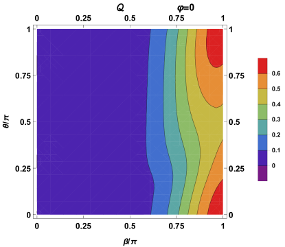
Figure 8: (Colour online) Plot of the nonlocality quantifier ${\cal Q}$ evaluated in the state $|\Psi_{3,2}\rangle$ of the SLOCC class $\{{\cal{D}}_{3,2}\}$, as a function of one of the state parameters $\beta$ and Charlie’s measurement orientations $\theta$. Here we have fixed $\phi=0$. It is seen that ${\cal Q}$ is non-zero in the entire range of the state parameter $0<\beta\leq\pi$ and reaches a maximum value $\approx 0.66$, when $\beta=\pi$ (which corresponds to the W state), $\theta=0,\pi$.

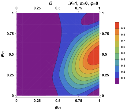
Figure 9: (Colour online) Plot of the nonlocality quantifier ${\cal Q}$ evaluated in the state $|\Psi_{3,3}\rangle\in\{{\cal{D}}_{3,3}\}$, as a function of $\beta$ and Charlie’s measurement orientations $\theta$; we have fixed the parameters $y=1,\alpha=0$ and chosen the measurement angle $\phi=0$. We find that ${\cal Q}$ is non-zero for the entire SLOCC class $\{{\cal{D}}_{3,3}\}$ and the maximum value ${\cal Q}=1$ is obtained when the parameter $\beta=\pi$ (which corresponds to the GHZ state) for the measurement angle $\theta=\pi/2$.

Recall that entanglement of the three qubit states belonging to the three distinct spinor SLOCC class $\{{\cal{D}}_{3,3}\}$ (see (8)) is characterized by the three-tangle $\tau$ and the pairwise concurrence $C$, expressed in terms of the state parameters $0<y\leq 1,0\leq\alpha\leq 2\pi,0<\beta\leq\pi$ as meyer

$$\tau=\frac{2y\sin^{3}(\beta/2)}{1+y^{2}+2y\,\cos^{3}(\beta/2)\cos\alpha}$$ (33)

$$C=\frac{y\sin(\beta)\,\sin(\beta/2)}{1+y^{2}+2y\,\cos^{3}(\beta/2)\cos\alpha}.$$ (34)

However, the three-tangle vanishes for the three qubit states belonging to the two distinct spinor class $\{{\cal{D}}_{3,2}\}$ and the pairwise concurrence is given by meyer

$$C=\frac{2-2\cos^{2}(\beta/2)}{3+6\cos^{2}(\beta/2)}.$$ (35)

Note that the nonlocality quantifier ${\cal Q}$ of the class $\{{\cal{D}}_{3,3}\}$ assumes its largest possible value in the GHZ state, characterized by the state parameters $y=1,\,\beta=\pi,\alpha=0$, (see (8)) for which the three-tangle attains its maximum value $\tau=1$ and the pairwise concurrence $C$ vanishes (see (33) and (34)). This indicates that the three-tangle $\tau$ plays a significant role in characterizing the non-locality of three qubit states of the SLOCC family $\{{\cal{D}}_{3,3}\}$ under the conditional-CHSH test. On the other hand, the the non-locality quantifier ${\cal Q}$ associated with the SLOCC class $\{{\cal{D}}_{3,2}\}$ attains its maximum value in the W state, governed by the state parameter $\beta=\pi$ for which the pairwise concurrence $C$ (see (35)) approaches its highest possible value. In other words, the conditional CHSH test indicates that genuine tripartite non-local correlations characterized by non-zero tangle are stronger than those characterized by pairwise concurrence. In the next section we proceed to explore non-locality of pure permutation symmetric three-qubit states using tight Bell inequalities in the (3,2,2) scenario.

5 Nonlocality of pure symmetric three-qubit states via tight Bell inequalities in the (3,2,2) scenario

In this section we discuss maximum nonlocality of pure entangled symmetric three-qubit states using the tight Bell inequalities in the (3,2,2) i.e., three-party, two-setting, two-outcome scenario pit01 ; silwa ; cab1 . Pitowsky and Svozil pit01 , Sliwa silwa had identified that there are exactly 46 inequivalent classes of tight Bell inequalities in the (3,2,2) scenario, which get maximally violated by entangled three-qubit states, when suitable local measurements are carried out. These 46 classes of tight Bell inequalities and their local maximum value have been listed in Table 1 of Ref. cab1 . It has been shown LMas that maximum violations of the tight Bell inequalities are attained by three-qubit pure states when local projective measurements are employed. In Ref. cab1 , explicit structure of the set of all entangled pure three-qubit states along with the optimal local observables and the corresponding quantum maximum value achievable in these states has been tabulated. We observe that six classes of these tight Bell inequalities i.e., 2, 5, 22, 26, 33 and 39 (see Table 2 of Ref. cab1 ) are maximally violated by pure permutation symmetric three-qubit states . We have listed these six classes of tight Bell inequalities, the optimal local dichotomic measurement settings $A_{i},\,B_{i},\,C_{i},i=1,2$ of Alice, Bob and Charlie, the three-qubit pure state $|\psi^{(k)}_{\rm ABC}\rangle,\ k=2,5,22,26,33,39$ in which maximum violation is witnessed are given in Table 1.

Table 1: A list of six different classes of tight Bell inequalities, labeled by 2, 5, 22, 26, 33 and 39, [see Tables I, IV and  V of Ref. cab1 for details on the 46 classes of tight Bell inequalities of the (3,2,2) scenario], corresponding local dichotomic observables $A_{i},\,B_{i},\,C_{i},i=1,2$ of Alice, Bob, Charlie, pure three-qubit states $|\psi^{(k)}_{\rm ABC}\rangle$ which maximally violate the inequalities, & the maximum quantum violation.

Class	Tight Bell inequality	State	Quantum
			maximum
2	$\left\langle(A_{1}\,B_{1}+A_{2}\,B_{2})\,C_{1}+(A_{2}\,B_{1}-A_{1}\,B_{2})\,C_{2}\right\rangle\leq 2,$ $A_{1}=\sigma_{3}\otimes I\otimes I,\,A_{2}=\sigma_{1}\otimes I\otimes I$ $B_{1}=I\otimes\sigma_{3}\otimes I,\,B_{2}=I\otimes\sigma_{1}\otimes I$ $C_{1}=I\otimes I\otimes\sigma_{3},\,C_{2}=I\otimes I\otimes\sigma_{1}$	$|\psi_{\rm ABC}^{(2)}\rangle=\frac{1}{\sqrt{2}}\left(|\tilde{+}\tilde{-}\tilde{-}\rangle+|\tilde{-}\tilde{+}\tilde{+}\rangle\right)$ $|\tilde{\pm}\rangle=\frac{1}{\sqrt{2}}(|0\rangle\pm i|1\rangle)$	4
5	$\left\langle(A_{1}+B_{1}+C_{1})+B_{1}\,C_{2}+B_{2}\,(C_{1}-C_{2})\right.$ $+A_{1}\,(B_{2}+C_{2}-B_{1}\,C_{1}-B_{1}\,C_{2}-B_{2}\,C_{1})$ $\left.+A_{2}\,(B_{1}+C_{1}-B_{2}-C_{2}-B_{1}\,C_{1}+B_{2}\,C_{2})\right\rangle\leq 3$ $A_{1}=o^{(5)}_{1}\otimes I\otimes I,\,A_{2}=\sigma_{1}\otimes I\otimes I$ $B_{1}=I\otimes o^{(5)}_{1}\otimes I,\,B_{2}=I\otimes\sigma_{1}\otimes I$ $C_{1}=I\otimes I\otimes o^{(5)}_{1},\,C_{2}=I\otimes I\otimes\sigma_{1}$ $o^{(5)}_{1}=\sqrt{-2+\sqrt{5}}\,(2\,\sigma_{3}+\sigma_{1})$	$|\psi_{\rm ABC}^{(5)}\rangle=a^{(5)}\,|\bar{+}\bar{+}\bar{+}\rangle+b^{(5)}\,|\bar{-}\bar{-}\bar{-}\rangle$            $+c^{(5)}\,|\bar{+}\bar{+}\bar{-}\rangle+d^{(5)}\,|\bar{+}\bar{-}\bar{+}\rangle+e^{(5)}\,|\bar{-}\bar{+}\bar{+}\rangle$ $a^{(5)}=-\left(-\frac{3}{2}+\frac{7}{2\,\sqrt{5}}\right)^{1/2},\,b^{(5)}=-\left(1-\frac{2}{\sqrt{5}}\right)^{1/2}$ $c^{(5)}=d^{(5)}=e^{(5)}=\left(\frac{1}{2}-\frac{1}{2\,\sqrt{5}}\right)^{1/2}$ $|\bar{\pm}\rangle=\frac{1}{\sqrt{2}}(-|0\rangle\pm|1\rangle)$	$8\sqrt{5}-13$
22	$\left\langle(A_{1}+B_{1}+C_{1})+(A_{2}+B_{2}+C_{2})+B_{1}\,C_{1}-B_{2}\,C_{2}\right.$ $+A_{1}\,(B_{1}+C_{1}-2\,B_{1}\,C_{1}-B_{2}\,C_{1}-B_{1}\,C_{2}+B_{2}\,C_{2})$ $\left.-A_{2}(B_{2}+C_{2}+B_{1}\,C_{1}-B_{1}\,C_{2}-B_{2}\,C_{1})\right\rangle\leq 4$ $A_{1}=o^{(22)}_{1}\otimes I\otimes I,\,A_{2}=o^{(22)}_{2}\otimes I\otimes I$ $B_{1}=I\otimes o^{(22)}_{1}\otimes I,\,B_{2}=I\otimes o^{(22)}_{2}\otimes I$ $C_{1}=I\otimes I\otimes o^{(22)}_{1},\,C_{2}=I\otimes I\otimes o^{(22)}_{2}$ $o^{(22)}_{1}=-0.25333\,\sigma_{1}+0.96738\,\sigma_{3}$ $o^{(22)}_{2}=0.99937\,\sigma_{1}+0.03540\,\sigma_{3}$	$|\psi_{\rm ABC}^{(22)}\rangle=a^{(22)}\,|000\rangle+b^{(22)}\,|111\rangle$ $\hskip 36.135pt+c^{(22)}\,|001\rangle+d^{(5)}\,|100\rangle+\rangle+e^{(5)}\,|010\rangle$ $a^{(22)}=0.161337,\,b^{(22)}=-0.664411$ $c^{(22)}=d^{(22)}=e^{(22)}=0.421319$	6.19794
26	$\left\langle(A_{1}+B_{1}+C_{1})+A_{1}(B_{1}+C_{1}-B_{1}\,C_{1}+2\,B_{2}\,C_{2})\right.$ $+2A_{2}\,(B_{2}+C_{2}-B_{1}\,C_{2}-B_{2}\,C_{1})$ $\left.+B_{1}\,C_{1}-2\,B_{2}\,C_{2}\right\rangle\leq 5$ $A_{1}=\sigma_{3}\otimes I\otimes I,\,A_{2}=\sigma_{1}\otimes I\otimes I$ $B_{1}=I\otimes\sigma_{3}\otimes I,\,B_{2}=I\otimes\sigma_{1}\otimes I$ $C_{1}=I\otimes I\otimes\sigma_{3},\,C_{2}=I\otimes I\otimes\sigma_{1}$	$|\psi_{\rm ABC}^{(26)}\rangle=\frac{1}{\sqrt{6}}\,(|001\rangle+|010\rangle)-|100\rangle)+\frac{1}{\sqrt{2}}|111\rangle$	$1+4\sqrt{3}$
33	$\left\langle(A_{1}+B_{1}+C_{1})+(A_{2}+B_{2}+C_{2})-B_{1}\,C_{2}-B_{2}\,C_{1}\right.$ $-A_{2}\,(B_{1}+C_{1}-B_{1}\,C_{2}-2\,B_{1}\,C_{1}-B_{2}\,C_{1}+3\,B_{2}\,C_{2})$ $\left.-A_{1}\,(B_{2}+C_{2}-2\,B_{1}\,C_{2}-2\,B_{2}\,C_{1}-B_{2}\,C_{2})\right\rangle\leq 6$ $A_{1}=o^{(33)}_{1}\otimes I\otimes I,\,A_{2}=o^{(33)}_{2}\otimes I\otimes I$ $B_{1}=I\otimes o^{(33)}_{1}\otimes I,\,B_{2}=I\otimes o^{(33)}_{2}\otimes I$ $C_{1}=I\otimes I\otimes o^{(33)}_{1},\,C_{2}=I\otimes I\otimes o^{(33)}_{2}$ $o^{(33)}_{1}=0.48263\,\sigma_{1}+0.87582\,\sigma_{3}$ $o^{(33)}_{2}=0.92087\,\sigma_{1}-0.38987\,\sigma_{3}$	$|\psi_{\rm ABC}^{(33)}\rangle=a^{(33)}\,|000\rangle+b^{(33)}\,|111\rangle$ $\hskip 36.135pt+c^{(33)}\,|001\rangle+d^{(33)}\,|100\rangle+e^{(33)}\,|010\rangle$ $a^{(33)}=-0.024223,\,b^{(33)}=-0.621262$, $c^{(33)}=d^{(33)}=e^{(33)}=0.452197$	9.78988
39	$\left\langle 2\,(A_{1}+B_{1}+C_{1})+B_{1}\,(C_{2}-C_{1})+B_{2}(C_{1}+C_{2})\right.$ $-A_{1}\,(B_{1}+C_{1}-B_{2}-C_{2})+A_{2}\,(B_{1}+C_{1}+B_{2}+C_{2})$ $+A_{1}(2\,B_{1}\,C_{1}-B_{1}\,C_{2}-\,B_{2}\,C_{1}-2\,B_{2}\,C_{2})$ $\left.-A_{2}\,(B_{1}\,C_{1}+2\,B_{1}\,C_{2}+2\,B_{2}\,C_{1}-B_{2}\,C_{2})\right\rangle\leq 6$ $A_{1}=o^{(39)}_{1}\otimes I\otimes I,\,A_{2}=o^{(39)}_{2}\otimes I\otimes I$ $B_{1}=I\otimes o^{(39)}_{1}\otimes I,\,B_{2}=I\otimes o^{(39)}_{2}\otimes I$ $C_{1}=I\otimes I\otimes o^{(39)}_{1},\,C_{2}=I\otimes I\otimes o^{(39)}_{2}$ $o^{(39)}_{1}=-0.04834\,\sigma_{1}-0.99883\,\sigma_{3}$ $o^{(39)}_{2}=-0.99683,\sigma_{1}+0.07953\,\sigma_{3}$	$|\psi_{\rm ABC}^{(39)}\rangle=a^{(39)}\,|000\rangle+b^{(39)}\,111\rangle$ $+c^{(39)}\,|001\rangle+d^{(39)}\,|100\rangle+e^{(39)}\,|010\rangle$ $a^{(39)}=0.177347,\,b^{(39)}=-0.386311,$ $c^{(39)}=d^{(39)}=e^{(39)}=0.522594$	9.32530

It is readily identified that the states $\psi^{(k)}_{\rm ABC}\rangle,\,k=2,5,22,26,33,39$ are local unitary equivalent to permutation symmetric states $|\psi^{(k)}_{\rm sym}\rangle$:

$${\cal U}^{(2)}\,|\psi^{(2)}_{\rm ABC}\rangle = |\psi^{(2)}_{\rm sym}\rangle=|{\rm GHZ}\rangle$$

$${\cal U}^{(5)}\,|\psi^{(5)}_{\rm ABC}\rangle = |\psi^{(5)}_{\rm sym}\rangle$$

$$= a^{(5)}\,|000\rangle+b^{(5)}\,|111\rangle+\sqrt{3}\,c^{(5)}\,|{\rm W}\rangle$$

$${\cal U}^{(0)}|\psi^{(22)}_{\rm ABC}\rangle = |\psi^{(22)}_{\rm sym}\rangle$$

$$= a^{(22)}\,|000\rangle+b^{(22)}\,|111\rangle+\sqrt{3}\,c^{(22)}\,|{\rm W}\rangle$$

$${\cal U}^{(26)}\,|\psi^{(26)}_{\rm ABC}\rangle = |\psi^{(26)}_{\rm sym}\rangle=-\frac{1}{\sqrt{2}}(|111\rangle+|{\rm W}\rangle)$$

$${\cal U}^{(0)}|\psi^{(33)}_{\rm ABC}\rangle = |\psi^{(33)}_{\rm sym}\rangle$$

$$= a^{(33)}\,|000\rangle+b^{(33)}\,|111\rangle+\sqrt{3}\,c^{(33)}\,|{\rm W}\rangle$$

$${\cal U}^{(0)}\,|\psi^{(39)}_{\rm ABC}\rangle = |\psi^{(39)}_{\rm sym}\rangle$$

$$= a^{(39)}\,|000\rangle+b^{(39)}\,|111\rangle+\sqrt{3}\,c^{(39)}\,|{\rm W}\rangle$$

where

$${\cal U}^{(0)} = I\otimes I\otimes I$$

$${\cal U}^{(2)} = U_{-}^{(2)}\otimes U_{+}^{(2)}\otimes U_{+}^{(2)};\ \ U_{\pm}^{(2)}=\frac{1}{\sqrt{2}}\left(\begin{array}[]{cc}1&\pm i\\ 1&\mp i\end{array}\right)$$

$${\cal U}^{(5)} = U^{(5)}\otimes U^{(5)}\otimes U^{(5)},\ U^{(5)}=\frac{1}{\sqrt{2}}\left(\begin{array}[]{cc}-1&1\\ -1&-1\end{array}\right)$$

$${\cal U}^{(26)} = \sigma_{3}\otimes I\otimes I$$

In Table 2 we have displayed the explicit forms of the distinct constituent spinors of the pure three-qubit symmetric states  $|\psi^{(k)}_{\rm sym}\rangle$, $k=2,\,5,\,22,\,26,\,33,\,39$. All these states belong to the three distinct spinor SLOCC class $\{{\cal{D}}_{3,3}\}.$ None of the tight Bell inequalities of the (3,2,2) scenario are maximally violated by permutations symmetric three-qubit pure states of the two distinct spinor class $\{{\cal{D}}_{3,2}\}$. On the other hand, there are six three-qubit pure symmetric states $|\psi^{(k)}_{\rm sym}\rangle$ $k=2,\,5,\,22,\,26,\,33,\,39$ of the SLOCC class $\{{\cal D}_{3,3}\}$, which maximally violate six classes of tight Bell inequalities (see Table 1). Violation of the tight Bell inequality ‘26’ by the three-qubit state $|\psi^{(26)}_{\rm ABC}\rangle$ has been experimentally verified recently cab2 .

Table 2: Three distinct spinors constituting the pure three-qubit symmetric states $|\psi^{(k)}_{\rm sym}\rangle$. The states $|\psi^{(k)}_{\rm sym}\rangle$ belong to the SLOCC class $\{{\cal D}_{3,3}\}$ of three distinct spinors and they maximally violate the tight Bell inequalities $k=2,\,5,\,22,\,26,\,33,\,39$ of the (3,2,2) scenario cab1 ).

Class	Three-qubit symmetric states $|\psi^{(k)}_{\rm sym}\rangle$ &
	the associated constituent spinors
2	$|\psi^{(2)}_{\rm sym}\rangle={\cal N}^{(2)}\,\sum_{P}\hat{P}\{|\,\phi\rangle_{1}\,\otimes|\,\phi\rangle_{2}\otimes|\phi\rangle_{3}\}=|{\rm GHZ}\rangle$
	$|\phi\rangle_{p}=\frac{1}{\sqrt{2}}(|0\rangle+\omega^{p}\,|1\rangle),p=1,2,3$ where $\omega^{3}=1$
	$|\psi^{(5)}_{\rm sym}\rangle={\cal N}^{(5)}\,\sum_{P}\hat{P}\{|\,\beta\rangle_{1}\,\otimes|\,\beta\rangle_{2}\otimes|\beta\rangle_{3}\}$
5	$|\beta\rangle_{1}=0.916\,|0\rangle+0.402\,|1\rangle,$ $|\beta\rangle_{2}=0.904\,|0\rangle-0.427\,|1\rangle$
	$|\beta\rangle_{3}=0.161\,|0\rangle-0.987\,|1\rangle$
	$|\psi^{(22)}_{\rm sym}\rangle={\cal N}^{(22)}\,\sum_{P}\hat{P}\{|\,\beta\rangle_{1}\,\otimes|\,\beta\rangle_{2}\otimes|\beta\rangle_{3}\}$
22	$|\beta\rangle_{1}=\,0.795|0\rangle+0.607\,|1\rangle,$ $|\beta\rangle_{3}=\,0.821|0\rangle-0.571\,|1\rangle$
	$|\beta\rangle_{2}=\,0.128|0\rangle+0.992\,|1\rangle$
	$|\psi^{(26)}_{\rm sym}\rangle={\cal N}^{(26)}\,\sum_{P}\hat{P}\{|\,\beta\rangle_{1}\,\otimes|\,\beta\rangle_{2}\otimes|\beta\rangle_{3}\}$
26	$|\beta\rangle_{1}=\,0.796|0\rangle+0.605\,|1\rangle$, $|\beta\rangle_{2}=\,0.796|0\rangle-0.605\,|1\rangle$
	$|\beta\rangle_{3}=|1\rangle$
	$|\psi^{(33)}_{\rm sym}\rangle={\cal N}^{(33)}\,\sum_{P}\hat{P}\{|\,\beta\rangle_{1}\,\otimes|\,\beta\rangle_{2}\otimes|\beta\rangle_{3}\}$
33	$|\beta\rangle_{1}=0.830\,|0\rangle+0.558\,|1\rangle$, $|\beta\rangle_{2}=0.826\,|0\rangle-0.562\,|1\rangle$
	$|\beta\rangle_{3}=0.0018\,|0\rangle-0.998\,|1\rangle$
	$|\psi^{(39)}_{\rm sym}\rangle={\cal N}^{(39)}\,\sum_{P}\hat{P}\{|\,\beta\rangle_{1}\,\otimes|\,\beta\rangle_{2}\otimes|\beta\rangle_{3}\}$
39	$|\beta\rangle_{1}=0.890\,|0\rangle+0.455\,|1\rangle$, $|\beta\rangle_{2}=0.900\,|0\rangle-0.435\,|1\rangle$
	$|\beta\rangle_{3}=0.113\,|0\rangle+0.994\,|1\rangle$

6 Summary

Different forms of Bell inequalities have been proposed for studying nonlocality of permutation symmetric multiqubit states lewenstein1 ; lewenstein2 . In this work, we have focused on the CHSH chsh and the conditional CHSH inequalities cavalcanti ; rchaves to investigate nonlocal features of pure three-qubit symmetric states. These states admit an elegant parametrization for different SLOCC classes based on Majorana geometric representation meyer . Making use of the explicit parametrization we prove that pairs of qubits drawn from a pure entangled three-qubit symmetric state (shared by Alice, Bob and Charlie) are CHSH local. In fact this property can be attributed to monogamy of CHSH-nonlocality Qin15 ; Hall17 . Our explicit verification $\langle{\rm CHSH}\rangle_{\rm opt}\leq 2$ by two-qubit correlations of the entire class of entangled pure symmetric three qubit states thus upholds CHSH monogamy property.

Continuing further we have shown that conditional CHSH inequalities cavalcanti ; rchaves are useful in activating nonlocality hidden in two-qubit correlations recorded by Alice and Bob, when they are conditioned by the dichotomic outcomes of Charlie’s measurement on his qubit. We have explicitly demonstrated that the permutation symmetric three qubit states belonging to both the two and three distinct spinor SLOCC classes $\{{\cal D}_{3,2}\}$, $\{{\cal D}_{3,3}\}$, violate the conditional CHSH inequalities $\langle{\rm CHSH}\rangle^{\rm con}_{c=1\,\rm opt}\leq 2$ and $\langle{\rm CHSH}\rangle^{\rm con}_{\rm opt}\leq 2$. We also illustrate that while states belonging to both $\{{\cal D}_{3,2}\}$, $\{{\cal D}_{3,3}\}$ can attain the maximum value $2\sqrt{2}$ for $\langle{\rm CHSH}\rangle^{\rm con}_{c=1\,\rm opt}$, the maximum value for $\langle{\rm CHSH}\rangle^{\rm con}_{\rm opt}$ achievable by the states belonging to $\{{\cal D}_{3,2}\}$, $\{{\cal D}_{3,3}\}$ are $2.552$ and $2\sqrt{2}$ respectively. This observation lead us to define a quantity $\cal Q$ which quantifies nonlocality in pure symmetric states belonging to $\{{\cal D}_{3,2}\}$ and $\{{\cal D}_{3,3}\}$. Three-qubit GHZ state belonging to $\{{\cal D}_{3,3}\}$ is seen to have ${\cal Q}=1$ thereby exhibiting maximum nonlocality. On the same token, we have shown ${\cal Q}\approx 0.66$ for three-qubit W state belonging to $\{{\cal D}_{3,2}\}$. Furthermore, we have shown that symmetric three-qubit states belonging to the three distinct spinor class $\{{\cal D}_{3,3}\}$ maximally violate six of the 46 classes of tight Bell inequalities in the (3,2,2) scenario. There are no tight Bell inequalities in the (3,2,2) scenario that are maximally violated by the two distinct spinor class $\{{\cal D}_{3,2}\}$. The nonlocality tests discussed here offer useful signatures to distinguish the quantum states belonging to the inequivalent SLOCC classes $\{{\cal D}_{3,2}\}$ and $\{{\cal D}_{3,3}\}$. We believe that our work motivates experimental tests on the violations of nonlocality by pure three-qubit symmetric states in different physical platforms.

References

• (1) Bell, J.S.: On the Einstein-Podolsky-Rosen Paradox. Physics 1, 195 (1964)
• (2) Clauser, J.F., Horne, M.A., Shimony, A., Holt, R.A.: Proposed Experiment to Test Local Hidden-Variable Theories, Phys. Rev. Lett. 23, 880 (1969)
• (3) Cavalcanti, D., Almeida, M.L., Scarani, V., Acin, A.: Quantum networks reveal quantum nonlocality. Nat. Commun. 2, 1 (2011)
• (4) Chaves, R., Acin, A., Aolita, L., Cavalcanti, D.: Detecting nonlocality of noisy multipartite states with the Clauser-Horne-Shimony-Holt inequality. Phys. Rev. A. 89, 042106 (2014)
• (5) Brunner, N., Cavalcanti, D., Pironio, S., Scarani, V., Wehner, S.: Bell nonlocality. Rev. Mod. Phys. 86, 419 (2014)
• (6) Tura, J., Augusiak, R., Sainz, A.B., Vértesi, T., Lewenstein M., Acin A.: Detecting non-locality in multipartite quantum systems with two-body correlation functions, Science 344, 1256 (2014)
• (7) Tura, J., Augusiak, R., Sainz, A.B., Lücke B., Klempt, C., Lewenstein, M., Acin A.: Nonlocality in many-body quantum systems detected with two-body correlators. Ann. Phys. 362, 370 (2015)
• (8) Sen (De) A., Sen, U., Wieśniak, M., Kaszlikowski, D., Żukowski, M.: Multiqubit W states lead to stronger nonclassicality than Greenberger-Horne-Zeilinger states. Phys. Rev. A 68, 062306 (2003)
• (9) Bastin, T., Krins, S., Mathonet, P., Godefroid, M., Lamata, L. Solano, F.: Operational Families of Entanglement Classes for Symmetric $N$-Qubit States. Phys. Rev. Lett., 103, 070503 (2009)
• (10) Usha Devi, A.R., Sudha, Rajagopal, A.K.: Majorana representation of symmetric multiqubit states, Quantum Inf. Proc. 11 685 (2012).
• (11) Wang, Z., Markham, D.: Nonlocality of Symmetric States. Phys. Rev. Lett. 108, 210407 (2012)
• (12) Korbicz, J.K., Gühne, O., Lewenstein, M., Haffner, H., Roos, C. F., Blatt, R.: Generalized spin-squeezing inequalities in $N$-qubit systems: Theory and experiment. Phys. Rev. A. 74, 052319 (2006)
• (13) Usha Devi, A.R., Uma, M.S., Prabhu, R., Sudha: Local Invariants and Pairwise Entanglement in Symmetric Multi-qubit System. Int. J. Mod. Phys. B. 20, 1917 (2006)
• (14) Usha Devi, A.R., Prabhu, R., Rajagopal, A.K.: Characterizing Multiparticle Entanglement in Symmetric $N$-Qubit States via Negativity of Covariance Matrices. Phys. Rev. Lett. 98, 060501 (2007)
• (15) Usha Devi, A.R., Prabhu, R., Rajagopal, A.K.: Collective multipolelike signatures of entanglement in symmetric $N$-qubit systems. Phys. Rev. A. 76, 012322 (2007)
• (16) Meill, A., Meyer, D.A.: Symmetric three-qubit-state invariants. Phys. Rev. A. 96, 062310 (2017)
• (17) Majorana, E.: Atomi Orientati in Campo Magnetico Variabile. Nuovo Cimento 9, 43 (1932)
• (18) Pitowsky, I., Svozil, K.: Optimal tests of quantum nonlocality. Phys. Rev. A. 64, 014102 (2001)
• (19) Śliwa, C.: Symmetries of the Bell correlation inequalities. Phys. Lett. A. 317, 165 (2003).
• (20) López-Rosa, S., Xu, Z.-P., Cabello, A.: Maximum nonlocality in the $(3,\,2,\,2)$ scenario. Phys. Rev. A. 94, 062121 (2016)
• (21) Anwer, H., Nawareg, M., Cabello, A., Bourennane, M.: Experimental test of maximal tripartite nonlocality using an entangled state and local measurements that are maximally incompatible. Phys. Rev. A. 100, 022104 (2019)
• (22) Popescu, S., Rohrlich, D.: Genuine quantum non-locality, Phys. Lett. A. 166, 293 (1992)
• (23) Horodecki, R., Horodecki, P., Horodecki, M.: Violating Bell inequality by mixed spin-12 states: necessary and sufficient condition. Phys. Lett. A. 200, 340 (1995)
• (24) Greenberger, D. M., Horne, M. A., Zeilinger A., in Bell’s Theorem, Quantum Theory, and Conceptions of the Universe, edited by M. Kafatos (Kluwer, Dordrecht, 1989)
• (25) Gisin, N.: Bell’s inequality holds for all non-product states, Phys. Lett. A. 154, 201 (1991).
• (26) Masanes, L.: Extremal quantum correlations for N parties with two dichotomic observables per site, arXiv:quant-ph/0512100
• (27) Qin, H.-H., Fei, S.-M., Li-Jost, X.: Trade-off relations of Bell violations among pairwise qubit systems. Phys. Rev. A. 92, 062339 (2015).
• (28) Cheng, S., Hall, M.J.W.: Anisotropic Invariance and the Distribution of Quantum Correlations. Phys. Rev. Lett. 118, 010401 (2017)