Groupwise Multimodal Image Registration
using Joint Total Variation

Abstract

In medical imaging it is common practice to acquire a wide range of modalities (MRI, CT, PET, etc.), to highlight different structures or pathologies. As patient movement between scans or scanning session is unavoidable, registration is often an essential step before any subsequent image analysis. In this paper, we introduce a cost function based on joint total variation for such multimodal image registration. This cost function has the advantage of enabling principled, groupwise alignment of multiple images, whilst being insensitive to strong intensity non-uniformities. We evaluate our algorithm on rigidly aligning both simulated and real 3D brain scans. This validation shows robustness to strong intensity non-uniformities and low registration errors for CT/PET to MRI alignment. Our implementation is publicly available at https://github.com/brudfors/coregistration-njtv.

1 Introduction

This paper concerns a fundamental task in medical image analysis: intermodal image registration. Its aim is to align scans that represent the same object, but have been acquired with different modalities (e.g., multiple repeats of the same MRI sequence, CT, PET). For intramodal registration (e.g., MRIs of the same sequence), the difference between scans can be assumed to be independent with Gaussian noise, so that the cost function reduces to the sum of squared differences [1, 2]. In contrast, the challenge in intermodal alignment comes from the fact that the scans are now no longer repeated measures of the same signal, precluding the use of a simple model of ‘measurement error’. However, the complementarity of the information in multimodal data are of crucial importance in a wide array of applications, from medical diagnosis to radiotherapy planning. Over the years, many automated registration algorithms have therefore been developed to tackle the problem of automated intermodal image alignment [3, 4].

Automated registration methods often optimise a transformation parameter of some cost function. The challenge lies in finding a cost function that has its optimum when images are perfectly aligned. The most commonly used cost functions are based on intensity cross-correlation [5, 6, 7], intensity differences [8, 9, 10] and information theory. The most popular functional from information theory is mutual information (MI; [11, 12, 13]), which considers voxels as independent conditioned on a joint intensity distribution. This distribution is often encoded non-parametrically from the joint image intensity histogram [11], but parametric Gaussian mixture models have also been used [14]. Normalised mutual information (NMI; [15]) was introduced to remove the dependency of MI to the size of the overlap between field-of-views (FOV). MI-based cost-functions have been shown to be robust and accurate for medical image registration [16]. However, they can fail in the face of large intensity inconsistencies [17, 18], which can be caused, e.g., by non-homogeneous transmission or reception of the MR signal. To reduce the dependency on the image intensities, registration approaches based on aligning edges have been investigated, which include gradient magnitude correlation [19], Canny filters [20] and normalised gradients dot product [21, 22].

In this paper we propose an edge-based cost function that is groupwise, finding its optimum when several gradient magnitude images are in alignment. In contrast to pairwise methods, groupwise registration defines a cost function over all images to be aligned. Such an approach should, in principle, lead to more optimal alignment due to reduced bias and increased number of registration features [23, 24, 25]. Our cost function introduces the joint total variation (JTV) functional in the context of image registration. This functional has previously been used for image reconstruction, first in computer vision [26, 27] and then in medical imaging [28, 29]. We evaluate our method on both simulated and real brain scans. This validation shows robustness to strong intensity non-uniformities (INUs) and low registration errors for groupwise, multimodal alignment.

2 Methods

Total Variation. The total variation (TV) of a differentiable function $f:\Omega\subset\mathbb{R}^{D}\rightarrow\mathbb{R}$ is the integral of the $\ell_{2}$-norm of its gradient:

$$\textstyle\small\operatorname{TV}(f)=\lambda\int_{\Omega}\left\lVert\bm{\nabla}f({\bf x})\right\rVert_{2}\mathrm{d}{\bf x},$$ (1)

where $\lambda$ is a scaling parameter that relates to the Laplace distribution, and $D=3$ for volumetric medical images. Patient images of different modalities can be conceptualised as a multi-channel acquisition. For such a vector-valued function, where the value domain is $\mathbb{R}^{C}$, two TV functionals that can be devised are:

$$\textstyle\small\operatorname{CTV}({\bf f}) =\sum_{c=1}^{C}\lambda_{c}\operatorname{TV}(f_{c}),$$ (2)

$$\operatorname{JTV}({\bf f}) =\int_{\Omega}\left\lVert\left(\lambda_{c}\bm{\nabla}f_{c}({\bf x})\right)_{1\leqslant c\leqslant C}\right\rVert_{2}\mathrm{d}{\bf x}.$$ (3)

Here, CTV denotes colour total variation, which considers channels independently [30], whereas JTV denotes joint total variation that applies the norm to the joint gradients over all channels [31]. By assuming that each channel is composed with a rigid transformation ${\bf R}_{c}:\Omega\rightarrow\Omega$, it can be shown that CTV is unsuitable as a cost function for image registration. Defining ${\bf u}={\bf R}_{c}{\bf x}$, integration by substitution gives:

$$\textstyle\small\int_{\Omega_{x}}f_{c}({\bf x})\mathrm{d}{\bf x}=\int_{\Omega_{u}}f_{c}({\bf u})|{\bf J}|\mathrm{d}{\bf u},$$ (4)

where $|{\bf J}|$ is the absolute value of the determinant of the Jacobian matrix of ${\bf u}$. As the determinant of a rigid transformation is one, we get $|{\bf J}|=1$. Hence, the value of an individual TV term does not change with the application of a rigid transformation, and therefore neither does the CTV term.

Normalised Joint Total Variation. Images are not continuous but discrete, and can be defined on non-overlapping domains. Let $\mathcal{F}=\{{\bf f}_{1},\dots,{\bf f}_{C}\}$ be a set of discrete images representing the same object, which may have different FOV and numbers of voxels. These images are made to represent continuous vector-valued signals by interpolation. An arbitrary image is chosen as fixed (e.g., $c=1$), and a mapping from the moving images to the fixed is given by:

$$\textstyle\small\bm{\xi}_{c}({\bf x})={\bf I}_{3,4}{\bf M}_{1}^{-1}{\bf R}_{c}{\bf M}_{c}\begin{bmatrix}{\bf x}\\ 1\end{bmatrix},\quad c=2,\ldots,C,\quad{\bf I}_{3,4}=\begin{bmatrix}1&0&0&0\\ 0&1&0&0\\ 0&0&1&0\end{bmatrix},$$ (5)

where ${\bf M}_{c}$ is the $c$th image’s subject voxel-to-world mapping (read from the scan’s NIfTI header). The JTV of the aligned signal can then be written as:

$$\textstyle\small\operatorname{JTV}(\mathcal{F},\mathcal{R})=\int_{\Omega}\left\lVert\left(\lambda_{c}\bm{\nabla}f_{c}\left(\bm{\xi}_{c}^{-1}({\bf y})\right)\right)_{1\leqslant c\leqslant C}\right\rVert_{2}\mathrm{d}{\bf y},$$ (6)

where $\mathcal{R}=({\bf R}_{1},\dots,{\bf R}_{C})$ are the set of rigid-body transformations to be estimated (except ${\bf R}_{1}={\bf I}$) and $\Omega_{f_{1}}$ is the domain of the fixed image. Values outside of the fixed image’s FOV are nulled, so that the JTV term only involves observed voxels. As interpolation has a significant impact on the gradients shape, it is prevented from biasing the optimum by removing the individual TV terms from the cost function in (3), arriving at the proposed, normalised joint total variation (NJTV) cost function:

$$\textstyle\small\operatorname{NJTV}({\mathcal{F},\mathcal{R}})=\sqrt{C}\times\operatorname{JTV}(\mathcal{F},\mathcal{R})-\operatorname{CTV}(\mathcal{F},\mathcal{R}).$$ (7)

Note that the JTV term has been modulated with the square root of the number of channels. This modulation is necessary for the cost function to find its optimum when all gradient magnitudes are in alignment (more details in Fig. 1); that is, to be applicable to image registration.

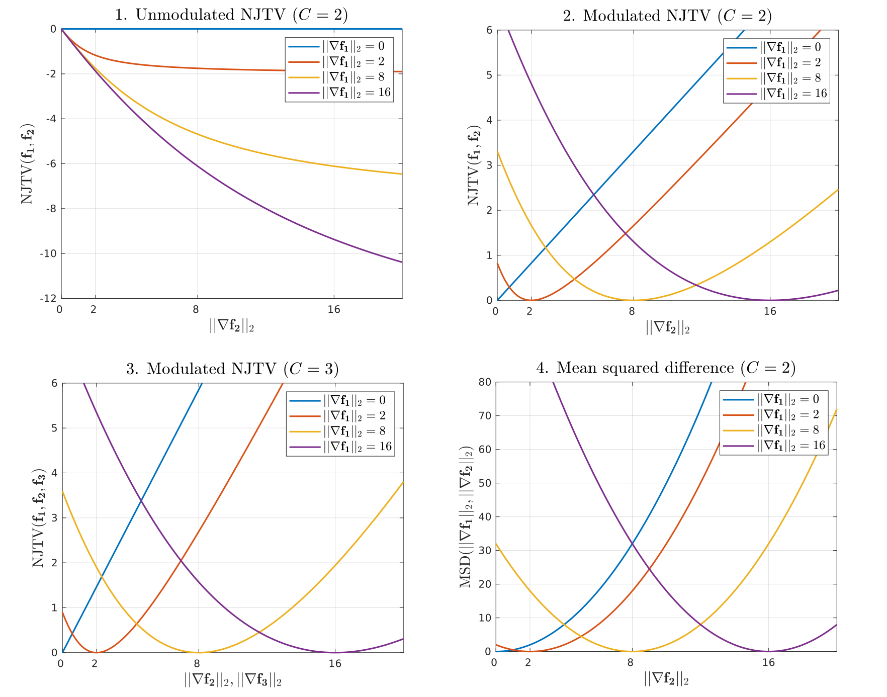
Figure 1: Behaviour of the NJTV cost function in (7). (1) By computing the NJTV for two voxels (${\bf f}_{1}$, ${\bf f}_{2}$) and changing the value of ${\bf f}_{2}$, whilst keeping the gradient magnitude ($||\nabla{\bf f_{1}}||_{2}$) fixed (for different values: $0,2,8,16$), it can be seen that NJTV it not minimised for the correct $||\nabla{\bf f_{1}}||_{2}$. (2) If we instead modulate by the square root of $C$, the correct minimum is reached. (3) Furthermore, computing modulated NJTV in a groupwise setting ($C=3$) also finds the correct minimum. (4) Mean squared difference between $||\nabla{\bf f_{1}}||_{2}$ and $||\nabla{\bf f_{2}}||_{2}$ is also minimised, but the curvatures are all the same. For NJTV, the curvatures vary: for values further from zero, the algorithm has more flexibility in the gradient magnitudes it matches with (an edge should match with an edge, but it matters less how strong the matching edges are); in contrast, if there is no gradient magnitude at a voxel (no edge), it reverts to a regular $\ell_{1}$ type penalty.

Lie Groups and Rigid-Body Transformations. We here consider rigid-body transforms in terms of their membership of the special Euclidean group in three dimensions SE(3). This group is a Lie group and can be equivalently encoded by its Lie algebra $\mathfrak{se}(3)$ [32]. Working with the Lie group representation of SE(3) gives a lower-dimensional, linear representation for rigid body motion. An orthonormal basis of the Lie algebra $\mathfrak{se}(3)$ is:

$$\textstyle\scriptsize\mathcal{B}=\begin{Bmatrix}&\begin{pmatrix}0&0&0&1\\ 0&0&0&0\\ 0&0&0&0\\ 0&0&0&0\end{pmatrix},&\begin{pmatrix}0&0&0&0\\ 0&0&0&1\\ 0&0&0&0\\ 0&0&0&0\end{pmatrix},&\begin{pmatrix}0&0&0&0\\ 0&0&0&0\\ 0&0&0&1\\ 0&0&0&0\end{pmatrix},&\frac{1}{2}\begin{pmatrix}0&1&0&0\\ \text{-}1&0&0&0\\ 0&0&0&0\\ 0&0&0&0\end{pmatrix},&\frac{1}{2}\begin{pmatrix}0&0&1&0\\ 0&0&0&0\\ \text{-}1&0&0&0\\ 0&0&0&0\end{pmatrix},&\frac{1}{2}\begin{pmatrix}0&0&0&0\\ 0&0&1&0\\ 0&\text{-}1&0&0\\ 0&0&0&0\end{pmatrix}\end{Bmatrix}.$$

A 3D rigid-body transform can be encoded by a vector ${\bf q}_{c}\in\mathbb{R}^{6}$ and recovered by matrix exponentiating the Lie algebra representation:

$$\textstyle\small{\bf R}_{{}_{c}}=\exp\left(\sum_{i=1}^{6}q_{ci}\mathcal{B}_{i}\right).$$ (8)

Conversely, by using a matrix logarithm, the encoding of a rigid-body matrix can be obtained by projecting it on the algebra:

$$\textstyle\small q_{i}=\operatorname{Tr}\left(\mathcal{B}_{i}\log({\bf R}_{c})^{\mathrm{T}}\right).$$ (9)

Implementation Details. The NJTV cost function in (7) is optimised using Powell’s method [33]. Powell’s method is an algorithm for finding a local minimum of a function by repeated 1D line-searches, where the function need not be differentiable, and no derivatives are taken. For improved runtime we compute the gradient magnitudes in (7) at the start of the algorithm, and interpolate them using second order b-splines. To avoid local optima and further improve runtime, a two-step coarse-to-fine scheme is used. The images are initially downsampled by a factor of eight and then registered. The algorithm is then run again using the parameters estimated from the previous registration (a warm start). The variable voxel size of the input images are accounted for in the computation of the gradients, by dividing each gradient direction with its voxel width. The scaling parameters, $\lambda_{1},\ldots,\lambda_{C}$, which normalise the cost function across modalities, are estimated from each individual image’s intensity histogram. If an image contains only positive values (e.g., an MR image), a two-class Rician mixture model is used and the scaling parameter is set as the mean of the non-background class. If an image also contains negative values (e.g., a CT image), a Gaussian mixture model is used instead. In order for the gradient magnitude to be independent from the data unit, the scaling parameter is set as the absolute difference between the mean of the background class and the mean of the foreground class. A random jitter is also introduced to the sampling grid of the fixed image to reduce interpolation artefacts [34].

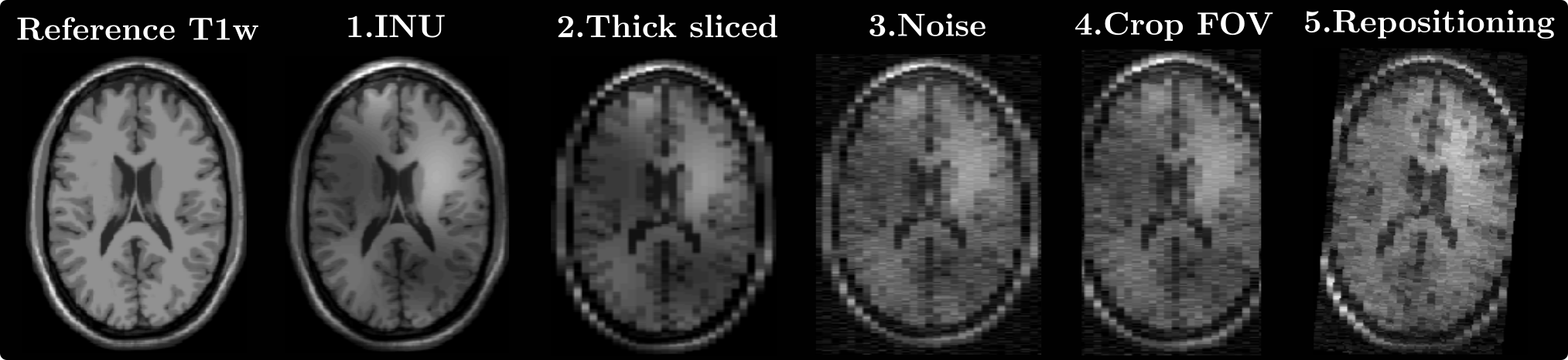
Figure 2: The BrainWeb simulation process, where one simulation includes a T1w, T2w and PDw scan. (1) Intensity non-uniformity (INU) is simulated by sampling smooth multiplicative scalar fields from a multivariate Gaussian distribution. (2) Thick-sliced data is simulated by downsampling the images, in one direction, by a factor 1 to 6. (3) A percentage of Rician noise is added, chosen uniformly between 0% and 50% of the maximum image intensity. (4) Partial brain coverage is simulated by cropping 20 mm on both sides in a randomly chosen anatomical direction. (5) Rigid repositioning is applied by uniformly sampled $x$-, $y$-, $z$-translations (between -50 and 50 mm) and $x$-, $y$-, $z$-rotations (between -15 and 15 degrees).

3 Validation

Registering BrainWeb Simulations. This section compares NJTV against other common cost functions, using non-degraded 1 mm isotropic T1-weighted (T1w), T2-weighted (T2w) and PD-weighted (PDw) images from the BrainWeb simulator [35]. A series of random degradations are applied to these reference scans, in order to make them more similar to clinical-grade data. These degradations are followed by a known rigid repositioning, which allows for a ground-truth comparison. Figure 2 details this process. The comparison includes the cost functions implemented in the co-registration routine of SPM12: MI [13, 36], NMI [15], entropy correlation coefficient (ECC; [36]), and normalised cross correlation (NCC; [5]). For NJTV, the alignment is optimised in a groupwise setting, whilst for the rest, one image is set as reference and all other images are aligned with this fixed reference. All cost functions use the the same optimisation stopping criteria and coarse-to-fine scheme (the defaults in SPM12). Each transform is encoded by three translations (in mm) and three Euler angles (in degrees). In total, $2,000$ simulations were performed. For each simulation, the error was computed between the estimated transformation parameters and the known ground-truths. The geometric mean and geometric standard deviation of absolute errors were then computed for each cost function. To evaluate the impact of different corruption parameters, a linear model was fitted to the log of the absolute translation errors generated by each method; with noise level, downsampling factor, INU magnitude and simulated offset as regressors. The corresponding maximum-likelihood slopes are written as $\beta_{n}$, $\beta_{d}$, $\beta_{i}$ and $\beta_{o}$.

The distribution of absolute errors is shown in Fig. 3. NJTV does consistently better ($\mu_{t}=0.048$ mm, $\mu_{r}=0.019$°), and NCC consistently worse ($\mu_{t}=0.69$ mm, $\mu_{r}=0.40$°), than all other approaches (MI: $\mu_{t}=0.12$ mm, $\mu_{r}=0.042$°; NMI: $\mu_{t}=0.12$ mm, $\mu_{r}=0.042$°; ECC: $\mu_{t}=0.12$ mm, $\mu_{r}=0.042$°), which are indistinguishable. Additionally, there are far fewer outliers with NJTV: a cut-off at 1 mm gives $97\%$ success for NJTV vs. 85% for MI, NMI and ECC and 60% for NCC. The slopes and intercepts of the log-linear fits are provided in Table 3, and illustrated for NJTV and MI in Fig. 4. NJTV is the method most impacted by noise ($\beta_{n}=2.91$, compared to MI’s $\beta_{n}=1.80$) and downsampling ($\beta_{d}=0.50$, compared to MI’s $\beta_{d}=0.31$), but the most robust to INUs ($\beta_{i}=0.059$, compared to MI’s $\beta_{i}=0.50$) and to original misalignment ($\beta_{o}=0.0044$, compared to MI’s $\beta_{o}=0.041$).

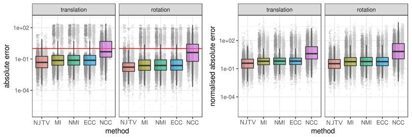
Figure 3: Absolute translation (mm) and rotation (deg) errors obtained from 2,000 BrainWeb simulations. Individual errors along the x, y, and z directions are plotted in different shades of grey, whereas the boxplot was computed from the pooled data. The vertical axis is in log-scale, so that higher points represent a greater error. The plot on the left shows absolute errors: errors below the red horizontal line are less than 1 mm or 1 deg. The plot on the right shows errors after normalisation by the geometric mean across methods.

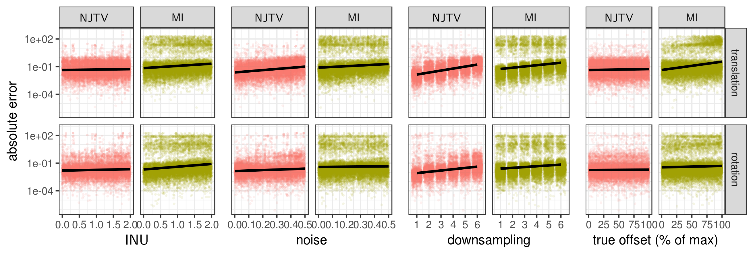
Figure 4: Absolute translation (mm) and rotation (deg) errors vs. INU strength, noise level, downsampling factor and true offset. Offsets are defined as percentages of the maximum simulated shift (50 mm / 15 deg). The vertical axis is in log-scale. Errors along each dimension are considered to be independent, and a regression line is plotted in black. NJTV, in contrast to MI, is immune to bias field and offset.

Table 1: Linear model fit to the results of the BrainWeb simulations. Shown are, for each method, the geometric mean (s.d.) of absolute translation and rotation errors (columns 2 and 3), as well as the coefficients of the linear fit log(abs(error)) $\scriptstyle\mathtt{\sim}$ 1 + INU + noise + downsampling + offset applied to translation errors (columns 4 to 7).

c — c c — c c c c c Method Tr. [mm] Rot. [deg] 1 INU Noise DS Offset
NJTV 0.048 (6.20) 0.019 (6.64) -5.68 0.059 2.91 0.50 0.0044
MI 0.12 (14.4) 0.042 (16.0) -5.18 0.50 1.80 0.31 0.041
NMI 0.12 (14.5) 0.042 (15.8) -5.22 0.53 1.76 0.33 0.040
ECC 0.12 (14.6) 0.042 (15.5) -5.19 0.45 2.12 0.33 0.041
NCC 0.69 (9.5) 0.40 (12.6) -1.47 0.21 0.13 0.14 0.015

Registering CT/PET to MRIs. The seminal RIRE multimodal registration challenge [37] compared a wide number of methods at rigidly registering CT/PET to MR scans (T1w, T2w, PDw). Among these were cost functions, such as normalised mutual information, that are still considered state-of-the-art over two decades later. In this section, NJTV is used to register the training patient of the RIRE dataset. In the original challenge, the algorithms were compared on scans from 18 held-out test patients. We here use the training patient’s scans, with known ground-truth corners, as it is currently not possible to submit new methods to the RIRE website (to obtain results on the test data). Ideally the testing data should have been used; however, this validation still gives an idea how NJTV performs on a multimodal registration task. Furthermore, as the algorithm does no learning, no such parameter optimisation can be done on the training patient. The results of the groupwise alignment is shown in Table 3. For CT/PET to MRI registration, the average of the median errors for all combinations of registrations was 2.0 mm, when all images were included in the groupwise registration. This alignment took less than 8 minutes on a modern workstation. When the groupwise alignment used only CT and MRIs, the error was 0.8 mm, whilst when only PET and MRIs were used it was 2.0 mm. The errors were computed as in [37]. The best methods from that paper achieved, on the test patients’ scans, a CT to MRI error below 2 mm, and a PET to MRI error of about 3 mm.

Table 2: NJTV registration errors for the RIRE training patient. Five scans (T1w, T2w, PDw, CT, PET) were groupwise aligned, rigidly, using three different combinations of scans: (top) all, (middle) CT and MRIs, (bottom) PET and MRIs. The median and maximum error were calculated from the difference between the eight estimated and ground-truth corner locations from the CT and PET scans, to the MRIs (in the $x$, $y$, $z$ directions, in mm).

c—ccc—ccc Error Median   Max
From/To T1w T2w PDw T1w T2w PDw
CT 2.2 1.7 2.3 8.5 7.2 9.6
PET 1.9 1.5 2.0 6.5 8.6 11.3
CT 1.4 0.4 0.7 3.3 2.3 3.5
PET 1.9 1.7 2.3 9.6 8.8 11.1

4 Conclusion

This paper introduced NJTV as a cost function for image registration. NJTV provides a principled method for performing accurate groupwise alignment. We show that NJTV is robust to strong INUs, and fails less often when faced with large misalignments. Powell’s method was here used to perform the NJTV optimisation. This method has the advantage of not requiring computing derivatives, but is therefore an inefficient optimisation scheme. Furthermore, it only works for cost functions with a small number of transformation parameters, such as affine registration. Future work will therefore investigate more efficient, derivative-based optimisation techniques, which could allow for groupwise nonlinear alignment using NJTV.

Acknowledgements:

MB was funded by the EPSRC-funded UCL Centre for Doctoral Training in Medical Imaging (EP/L016478/1) and the Department of Health’s NIHR-funded Biomedical Research Centre at University College London Hospitals. YB was funded by the MRC and Spinal Research Charity through the ERA-NET Neuron joint call (MR/R000050/1). MB and JA were funded by the EU Human Brain Project’s Grant Agreement No 785907 (SGA2).

References

- [1] P. Gerlot-Chiron and Y. Bizais, “Registration of multimodality medical images using a region overlap criterion,” Graphical Models and Image Processing, vol. 54, no. 5, pp. 396–406, 1992.
- [2] J. Ashburner, P. Neelin, D. Collins, A. Evans, and K. Friston, “Incorporating prior knowledge into image registration,” NeuroImage, vol. 6, no. 4, pp. 344–352, 1997.
- [3] D. L. Hill, P. G. Batchelor, M. Holden, and D. J. Hawkes, “Medical image registration,” Physics in medicine & biology, vol. 46, no. 3, p. R1, 2001.
- [4] F. P. Oliveira and J. M. R. Tavares, “Medical image registration: a review,” Computer methods in biomechanics and biomedical engineering, vol. 17, no. 2, pp. 73–93, 2014.
- [5] J. P. Lewis, “Fast template matching,” in Vision Interface, vol. 95, pp. 15–19, 1995.
- [6] A. V. Cideciyan, “Registration of ocular fundus images: an algorithm using cross-correlation of triple invariant image descriptors,” IEEE Engineering in Medicine and Biology Magazine, vol. 14, no. 1, pp. 52–58, 1995.
- [7] A. Roche, G. Malandain, X. Pennec, and N. Ayache, “The correlation ratio as a new similarity measure for multimodal image registration,” in MICCAI, vol. 1496, pp. 1115–1124, 1998.
- [8] J. V. Hajnal, N. Saeed, A. Oatridge, E. J. Williams, I. R. Young, and G. M. Bydder, “Detection of subtle brain changes using subvoxel registration and subtraction of serial MR images,” Journal of Computer Assisted Tomography, vol. 19, no. 5, pp. 677–691, 1995.
- [9] R. P. Woods, S. T. Grafton, C. J. Holmes, S. R. Cherry, and J. C. Mazziotta, “Automated image registration: I. general methods and intrasubject, intramodality validation,” Journal of Computer Assisted Tomography, vol. 22, no. 1, pp. 139–152, 1998.
- [10] A. Myronenko and X. Song, “Intensity-based image registration by minimizing residual complexity,” IEEE Transactions on Medical Imaging, vol. 29, no. 11, pp. 1882–1891, 2010.
- [11] A. Collignon, F. Maes, D. Delaere, D. Vandermeulen, P. Suetens, and G. Marchal, “Automated multi-modality image registration based on information theory,” in IPMI, vol. 3, pp. 263–274, 1995.
- [12] P. Viola and W. M. Wells III, “Alignment by maximization of mutual information,” International Journal of Computer Vision, vol. 24, no. 2, pp. 137–154, 1997.
- [13] W. M. Wells III, P. Viola, H. Atsumi, S. Nakajima, and R. Kikinis, “Multi-modal volume registration by maximization of mutual information,” Medical Image Analysis, vol. 1, no. 1, pp. 35–51, 1996.
- [14] J. Orchard and R. Mann, “Registering a multisensor ensemble of images,” IEEE Transactions on Image Processing, vol. 19, no. 5, pp. 1236–1247, 2009.
- [15] C. Studholme, D. L. Hill, and D. J. Hawkes, “An overlap invariant entropy measure of 3d medical image alignment,” Pattern recognition, vol. 32, no. 1, pp. 71–86, 1999.
- [16] J. P. Pluim, J. A. Maintz, and M. A. Viergever, “Mutual-information-based registration of medical images: a survey,” IEEE Transactions on Medical Imaging, vol. 22, no. 8, pp. 986–1004, 2003.
- [17] Z. S. Saad, D. R. Glen, G. Chen, M. S. Beauchamp, R. Desai, and R. W. Cox, “A new method for improving functional-to-structural MRI alignment using local Pearson correlation,” Neuroimage, vol. 44, no. 3, pp. 839–848, 2009.
- [18] D. N. Greve and B. Fischl, “Accurate and robust brain image alignment using boundary-based registration,” Neuroimage, vol. 48, no. 1, pp. 63–72, 2009.
- [19] J. B. A. Maintz, P. A. van den Elsen, and M. A. Viergever, “Comparison of edge-based and ridge-based registration of CT and MR brain images,” Medical Image Analysis, vol. 1, no. 2, pp. 151–161, 1996.
- [20] J. Orchard, “Globally optimal multimodal rigid registration: an analytic solution using edge information,” in IEEE International Conference on Image Processing, vol. 1, pp. I–485, IEEE, 2007.
- [21] E. Haber and J. Modersitzki, “Intensity gradient based registration and fusion of multi-modal images,” in MICCAI, pp. 726–733, Springer, 2006.
- [22] P. Snape, S. Pszczolkowski, S. Zafeiriou, G. Tzimiropoulos, C. Ledig, and D. Rueckert, “A robust similarity measure for volumetric image registration with outliers,” Image Vision Computing, vol. 52, pp. 97–113, 2016.
- [23] C. Wachinger, W. Wein, and N. Navab, “Three-dimensional ultrasound mosaicing,” in International Conference on Medical Image Computing and Computer-Assisted Intervention, pp. 327–335, Springer, 2007.
- [24] Ž. Spiclin, B. Likar, and F. Pernus, “Groupwise registration of multimodal images by an efficient joint entropy minimization scheme,” IEEE Transactions on Image Processing, vol. 21, no. 5, pp. 2546–2558, 2012.
- [25] M. Polfliet, S. Klein, W. Huizinga, M. M. Paulides, W. J. Niessen, and J. Vandemeulebroucke, “Intrasubject multimodal groupwise registration with the conditional template entropy,” Medical Image Analysis, vol. 46, pp. 15–25, 2018.
- [26] X. Bresson and T. F. Chan, “Fast dual minimization of the vectorial total variation norm and applications to color image processing,” Inverse problems and imaging, vol. 2, no. 4, pp. 455–484, 2008.
- [27] C. Wu and X.-C. Tai, “Augmented Lagrangian method, dual methods, and split Bregman iteration for ROF, vectorial TV, and high order models,” SIAM Journal on Imaging Sciences, vol. 3, no. 3, pp. 300–339, 2010.
- [28] J. Huang, C. Chen, and L. Axel, “Fast multi-contrast MRI reconstruction,” Magnetic resonance imaging, vol. 32, no. 10, pp. 1344–1352, 2014.
- [29] M. Brudfors, Y. Balbastre, P. Nachev, and J. Ashburner, “MRI super-resolution using multi-channel total variation,” in MIUA, pp. 217–228, Springer, 2018.
- [30] P. Blomgren and T. F. Chan, “Color tv: total variation methods for restoration of vector-valued images,” IEEE transactions on image processing, vol. 7, no. 3, pp. 304–309, 1998.
- [31] G. Sapiro and D. L. Ringach, “Anisotropic diffusion of multivalued images with applications to color filtering,” IEEE Transactions on Image Processing, vol. 5, no. 11, pp. 1582–1586, 1996.
- [32] R. P. Woods, “Characterizing volume and surface deformations in an atlas framework: theory, applications, and implementation,” NeuroImage, vol. 18, no. 3, pp. 769–788, 2003.
- [33] W. H. Press, S. A. Teukolsky, W. T. Vetterling, and B. P. Flannery, Numerical recipes 3rd edition: the art of scientific computing. Cambridge university press, 2007.
- [34] M. Unser and P. Thévenaz, “Stochastic sampling for computing the mutual information of two images,” in Proceedings of the 5th International Workshop on Sampling Theory and Applications (SampTA’03), pp. 102–109, 2003.
- [35] C. A. Cocosco, V. Kollokian, R. K.-S. Kwan, G. B. Pike, and A. C. Evans, “BrainWeb: online interface to a 3D MRI simulated brain database,” in NeuroImage, Citeseer, 1997.
- [36] F. Maes, A. Collignon, D. Vandermeulen, G. Marchal, and P. Suetens, “Multimodality image registration by maximization of mutual information,” IEEE Transactions on Medical Imaging, vol. 16, no. 2, pp. 187–198, 1997.
- [37] J. B. West, , and R. P. Woods, “Comparison and evaluation of retrospective intermodality image registration techniques,” in Medical Imaging 1996: Image Processing, vol. 2710, pp. 332–348, SPIE, 1996.