Green functions and propagation in the Bopp-Podolsky electrodynamics

Abstract

In this paper, we investigate the so-called Bopp-Podolsky electrodynamics. The Bopp-Podolsky electrodynamics is a prototypical gradient field theory with weak nonlocality in space and time. The Bopp-Podolsky electrodynamics is a Lorentz and gauge invariant generalization of the Maxwell electrodynamics. We derive the retarded Green functions, first derivatives of the retarded Green functions, retarded potentials, retarded electromagnetic field strengths, generalized Liénard-Wiechert potentials and the corresponding electromagnetic field strengths in the framework of the Bopp-Podolsky electrodynamics for three, two and one spatial dimensions. We investigate the behaviour of these electromagnetic fields in the neighbourhood of the light cone. In the Bopp-Podolsky electrodynamics, the retarded Green functions and their first derivatives show fast decreasing oscillations inside the forward light cone.

Keywords: Bopp-Podolsky electrodynamics; Green function; propagation; retardation; retarded potentials; Liénard-Wiechert potentials

Wave Motion 91 (2019), 102388; https://doi.org/10.1016/j.wavemoti.2019.102388

1 Introduction

Generalized continuum theories such as gradient theories and nonlocal theories are exciting and challenging research fields in physics, applied mathematics, material science and engineering science (see, e.g., [1, 2, 3, 4, 6, 5, 7, 8, 9, 10]). Gradient theories and nonlocal theories possess characteristic internal length scales in order to describe size-effects. Such generalized continuum theories are able to provide a regularization of the singularities present in classical continuum theories which are not valid at short distances. Generalized continuum theories are continuum theories valid at small scales.

In physics, an important and useful gradient theory is the so-called Bopp-Podolsky electrodynamics, which is the gradient theory of electrodynamics containing one length scale parameter, $\ell$, the so-called Bopp-Podolsky parameter. Bopp [1] and Podolsky [3] have proposed such a gradient theory representing a classical generalization of the Maxwell electrodynamics towards a generalized electrodynamics with linear field equations of fourth order in order to avoid singularities in the electromagnetic fields and to have a finite and positive self-energy of point charges (see also [4, 11, 12]). Due to its simplicity, the Bopp-Podolsky theory can be considered as the prototype of a gradient theory. Therefore, the Bopp-Podolsky electrodynamics represents the simplest, physical gradient field theory with weak nonlocality in space and time.

Nowadays there is a renewed interest in the Bopp-Podolsky electrodynamics (e.g., [13, 14]), in particular to solve the long-outstanding problem of the electromagnetic self-force of a charged particle present in the classical Maxwell electrodynamics which goes back to Lorentz, Abraham and Dirac trying to formulate a classical theory of the electron. The equation of motion in the classical theory of the electron, often called the Lorentz-Dirac equation, is of third order in the time-derivative of the particle position, and as result it shows unphysical behaviour such as run-away solutions and pre-acceleration (see, e.g., the books by Rohrlich [15] and Spohn [16]). Therefore, the classical Maxwell electrodynamics in vacuum does not lead to a consistent equation of motion of charged point particles and a generalized electrodynamics could solve this problem.

In the static case, gradient electrostatics with generalized Coulomb law was given by Bopp [1], Podolsky [3], Landé and Thomas [12] and gradient magnetostatics including the generalized Biot-Savart law was given by Lazar [17]. Such generalized electrostatics and generalized magnetostatics have a physical meaning if the classical electric and magnetic fields are recovered in the limit $\ell\rightarrow 0$. In gradient electrostatics, for a point charge the electric potential is finite and non-singular, but the electric field strength is finite and discontinuous at the position of the point charge.

The Bopp-Podolsky theory has many interesting features. It solves the problem of infinite self-energy in the electrostatic case, and it gives the correct expression for the self-force of charged particles at short distances eliminating the singularity when $r\rightarrow 0$ as shown by  Frenkel [18], Zayats [13], Gratus et al. [14]. In this manner, the Bopp-Podolsky electrodynamics is free of classical divergences. Using the Bopp-Podolsky electrodynamics, Frenkel [18] solved the so-called $4/3$ problem of the electromagnetic mass in the Abraham-Lorentz theory, and Frenkel and Santos [19] eliminated runaway solutions from the Lorentz-Dirac equation of motion. These features allow experiments that could test the generalized electrodynamics as a viable effective field theory (e.g., [20]) and the Bopp-Podolsky electrodynamics offers the possibilities of the physical modeling at small scales. Iwanenko and Sokolow [11], Kvasnica [21] and Cuzinatto et al. [20] argued that the Bopp-Podolsky length scale parameter $\ell$ is in the order of $\sim 10^{-15}$  m, that means femtometre (fm), or even smaller. From the mathematical point of view, the length parameter $\ell$ plays the role of the regularization parameter in the Bopp-Podolsky electrodynamics. This length scale is associated to the massive mode, $m_{\text{BP}}$, of the Bopp-Podolsky electrodynamics through $m_{\text{BP}}=\hbar/(c\ell)$. Moreover, it is interesting to note that the Bopp-Podolsky electrodynamics is the only linear generalization of the Maxwell electrodynamics whose Lagrangian, containing second order derivatives of the electromagnetic gauge potentials, is both Lorentz and $U(1)$-gauge invariant [22].

The Bopp-Podolsky electrodynamics is akin to the Pauli-Villars regularization procedure used in quantum electrodynamics (see, e.g., [21, 23, 13, 24]). Therefore, the Bopp-Podolsky electrodynamics provides a regularization of the Maxwell electrodynamics based on higher order partial differential equations. On the other hand, Santos [25] analyzed the wave propagation in the vacuum of the Bopp-Podolsky electrodynamics and two kinds of waves were found: the classical non-dispersive wave of the Maxwell electrodynamics, and a dispersive wave reminiscent of wave propagation in a collisionless plasma with plasma (angular) frequency $\omega_{p}=c/\ell$, described by a Klein-Gordon equation.

In the Maxwell electrodynamics, quantities like the retarded potentials, the retarded electromagnetic field strengths, the Liénard-Wiechert potentials and the electromagnetic field strengths in the Liénard-Wiechert form are the basic fields and quantities for the classical electromagnetic radiation (see, e.g., [26, 27, 28]). In particular, the Liénard-Wiechert form of the electromagnetic field strengths is important for the calculation of the self-force of a charged point particle. In the Bopp-Podolsky electrodynamics, only a little is known for such fields necessary for the electromagnetic radiation and radiation reaction in the generalized electrodynamics of Bopp and Podolsky and their behaviour on the light cone (see, e.g., [29, 13, 14]). Only, the three-dimensional generalized Liénard-Wiechert potentials were given by Landé and Thomas [29] and the corresponding three-dimensional electromagnetic fields of a point charge have been recently given by Gratus et al. [14], for the first time. The aim of the present work is to close this gap and to give a systematic derivation and presentation of all important quantities in three, two and one spatial dimensions (3D, 2D, 1D). In particular, this work gives, for the first time, the analytical expressions for the retarded potentials and retarded electromagnetic fields in 2D and 1D, and for the generalized Liénard-Wiechert potentials and corresponding electromagnetic fields of a non-uniformly moving charge in 2D and 1D in the framework of the Bopp-Podolsky electrodynamics. This completes the library of all important field solutions needed in the Bopp-Podolsky electrodynamics in 3D, 2D, and 1D, which is a necessary step towards completing the study of the Bopp-Podolsky electrodynamics. In particular, we investigate the behaviour of these fields near and on the light cone.

The purpose of this paper is to add relevant results of the Green functions, retardation and wave propagation in the Bopp-Podolsky electrodynamics. In Section 2, we review the basic equations of the Bopp-Podolsky electrodynamics. In Section 3, we give a systematic derivation and collection of the (dynamical) Bopp-Podolsky Green function and its first derivatives in 3D, 2D and 1D in the framework of generalized functions. The retarded potentials and retarded electromagnetic field strengths are given in Section 4 for 3D, 2D and 1D. In Section 5, we present the generalized Liénard-Wiechert potentials and electromagnetic field strengths in generalized Liénard-Wiechert form. The paper closes with the conclusion in Section 6.

2 Basic framework of the Bopp-Podolsky electrodynamics

In the Bopp-Podolsky electrodynamics [1, 3], the electromagnetic fields are described by the Lagrangian density

$${\cal L_{\text{BP}}} =\frac{\varepsilon_{0}}{2}\,\Big{(}\bm{E}\cdot\bm{E}+\ell^{2}\nabla\bm{E}:\nabla\bm{E}-\frac{\ell^{2}}{c^{2}}\,\partial_{t}\bm{E}\cdot\partial_{t}\bm{E}\Big{)}$$

$$\ -\frac{1}{2\mu_{0}}\,\Big{(}\bm{B}\cdot\bm{B}+\ell^{2}\nabla\bm{B}:\nabla\bm{B}-\frac{\ell^{2}}{c^{2}}\,\partial_{t}\bm{B}\cdot\partial_{t}\bm{B}\Big{)}-\rho\phi+\bm{J}\cdot\bm{A}\,,$$ (1)

with the notation $\nabla\bm{E}:\nabla\bm{E}=\partial_{j}E_{i}\partial_{j}E_{i}$ and $\bm{E}\cdot\bm{E}=E_{i}E_{i}$. Eq. (2) corresponds to Bopp’s form of the Lagrangian [1]. Here $\phi$ and ${\bm{A}}$ are the electromagnetic gauge potentials, ${\bm{E}}$ is the electric field strength vector, ${\bm{B}}$ is the magnetic field strength vector, $\rho$ is the electric charge density, and ${\bm{J}}$ is the electric current density vector. $\varepsilon_{0}$ is the electric constant and $\mu_{0}$ is the magnetic constant (also called permittivity of vacuum and permeability of vacuum, respectively). The speed of light in vacuum is given by

$$c=\frac{1}{\sqrt{\varepsilon_{0}\mu_{0}}}\,.$$ (2)

Moreover, $\ell$ is the characteristic length scale parameter in the Bopp-Podolsky electrodynamics, $\partial_{t}$ denotes the differentiation with respect to the time $t$ and $\nabla$ is the Nabla operator. From the mathematical point of view, the characteristic length parameter $\ell$ plays the role of a regularization parameter in the Bopp-Podolsky theory. In addition to the classical terms, first spatial- and time-derivatives of the electromagnetic field strengths (${\bm{E}}$, ${\bm{B}}$) multiplied by the characteristic length $\ell$ and a characteristic time $T=\ell/c$, respectively, appear in Eq. (2) which describe a weak nonlocality in space and time. The limit $\ell\rightarrow 0$ is the limit from the Bopp-Podolsky electrodynamics to the Maxwell electrodynamics.

The electromagnetic field strengths (${\bm{E}}$, ${\bm{B}}$) can be expressed in terms of the electromagnetic gauge potentials (scalar potential $\phi$, vector potential ${\bm{A}}$)

$${\bm{E}} =-\nabla\phi-\partial_{t}\bm{A}\,,$$ (3)

$${\bm{B}} =\nabla\times\bm{A}\,.$$ (4)

Due to their mathematical structure, the electromagnetic field strengths (3) and (4) satisfy the two electromagnetic Bianchi identities (or electromagnetic compatibility conditions)

$$\nabla\times{\bm{E}}+\partial_{t}{\bm{B}} =0\,,$$ (5)

$$\nabla\cdot{\bm{B}} =0\,,$$ (6)

which are known as homogeneous Maxwell equations.

The Euler-Lagrange equations of the Lagrangian (2) with respect to the scalar potential $\phi$ and the vector potential $\bm{A}$ give the electromagnetic field equations

$$\big{[}1+\ell^{2}\square\big{]}\,\nabla\cdot\bm{E}=\frac{1}{\varepsilon_{0}}\,\rho\,,$$ (7)

$$\big{[}1+\ell^{2}\square\big{]}\Big{(}\nabla\times\bm{B}-\frac{1}{c^{2}}\,\partial_{t}\bm{E}\Big{)}=\mu_{0}\,{\bm{J}}\,,$$ (8)

respectively. The d’Alembert operator is defined as

$$\square:=\frac{1}{c^{2}}\,\partial_{tt}-\Delta\,,$$ (9)

where $\Delta$ is the Laplace operator. Eqs. (7) and (8) represent the generalized inhomogeneous Maxwell equations in the Bopp-Podolsky electrodynamics. In addition, the electric current density vector and the electric charge density fulfill the continuity equation

$$\nabla\cdot{\bm{J}}+\partial_{t}\rho=0\,.$$ (10)

If we use the variational derivative with respect to the electromagnetic fields ($\bm{E}$, $\bm{B}$), we obtain the constitutive relations in the Bopp-Podolsky electrodynamics for the response quantities ($\bm{D}$, $\bm{H}$) in vacuum

$${\bm{D}} :=\frac{\delta{\cal L_{\text{BP}}}}{\delta{\bm{E}}}=\varepsilon_{0}\,\big{[}1+\ell^{2}\square\big{]}{\bm{E}}\,,$$ (11)

$${\bm{H}} :=-\frac{\delta{\cal L_{\text{BP}}}}{\delta{\bm{B}}}=\frac{1}{\mu_{0}}\,\big{[}1+\ell^{2}\square\big{]}{\bm{B}}\,,$$ (12)

where ${\bm{D}}$ is the electric displacement vector (electric excitation), ${\bm{H}}$ is the magnetic excitation vector. The second terms in Eqs. (11) and (12) describe the polarization of the vacuum present in the Bopp-Podolsky electrodynamics. The vacuum in the Bopp-Podolsky electrodynamics is a classical vacuum plus vacuum polarization that behaves like a plasma-like vacuum [25].

Using the constitutive relations (11) and (12), the Euler-Lagrange equations (7) and (8) can be rewritten in the form of inhomogeneous Maxwell equations

$$\nabla\cdot{\bm{D}} =\rho\,,$$ (13)

$$\nabla\times{\bm{H}}-\partial_{t}{\bm{D}} ={\bm{J}}\,.$$ (14)

From Eqs. (7) and (8), inhomogeneous Bopp-Podolsky equations, being partial differential equations of fourth order, follow for the electromagnetic field strengths

$$\big{[}1+\ell^{2}\square\big{]}\square\,{\bm{E}} =-\frac{1}{\varepsilon_{0}}\Big{(}\nabla\rho+\frac{1}{c^{2}}\,\partial_{t}{\bm{J}}\Big{)}\,,$$ (15)

$$\big{[}1+\ell^{2}\square\big{]}\square\,{\bm{B}} =\mu_{0}\,\nabla\times{\bm{J}}\,.$$ (16)

Using the generalized Lorentz gauge condition [30]

$$\big{[}1+\ell^{2}\square\big{]}\left(\frac{1}{c^{2}}\,\partial_{t}\phi+\nabla\cdot\bm{A}\right)=0\,,$$ (17)

the electromagnetic gauge potentials fulfill the following inhomogeneous Bopp-Podolsky equations

$$\big{[}1+\ell^{2}\square\big{]}\square\,\phi =\frac{1}{\varepsilon_{0}}\,\rho\,,$$ (18)

$$\big{[}1+\ell^{2}\square\big{]}\square\,\bm{A} =\mu_{0}\,{\bm{J}}\,.$$ (19)

Note that the generalized Lorentz gauge condition (17) is as natural in the Bopp-Podolsky electrodynamics as the Lorentz gauge condition is in the Maxwell electrodynamics [30]. As shown by Galvão and Pimentel [30], the usual Lorentz gauge condition, $\frac{1}{c^{2}}\,\partial_{t}\phi+\nabla\cdot\bm{A}=0$, does not satisfy the necessary requirements for a consistent gauge in the Bopp-Podolsky electrodynamics: it does not fix the gauge, it is not preserved by the equations of motion, and it is not attainable. The generalized Lorentz gauge condition is also necessary in the quantization of the Bopp-Podolsky electrodynamics leading to a generalized quantum electrodynamics [31, 32]. Bufalo et al. [31] found that in such a generalized quantum electrodynamics, using the one-loop approximation, the electron self-energy and the vertex function are both ultraviolet finite.

3 Green function of the Bopp-Podolsky equation

The Bopp-Podolsky electrodynamics is a linear theory with partial differential equations of fourth order. Therefore, the powerful method of Green functions (fundamental solutions) can be used to construct exact analytical solutions.

The Green function $G^{\rm BP}$ of the Bopp-Podolsky equation, which is a partial differential equation of fourth order, is defined by

$$\big{[}1+\ell^{2}\square\big{]}\square\,G^{\rm BP}(\bm{R},\tau)=\delta(\tau)\delta(\bm{R})\,,$$ (20)

where $\tau=t-t^{\prime}$, $\bm{R}=\bm{r}-\bm{r}^{\prime}$ and $\delta$ is the Dirac $\delta$-function. Therefore, the Green function, $G^{\rm BP}$, is the fundamental solution of the linear hyperbolic differential operator of fourth order, $[1+\ell^{2}\square\big{]}\square$, in the sense of Schwartz’ distributions (or generalized functions) [33]. Because we are only interested in the retarded Green function, the causality constraint must be fulfilled

$$G^{\rm BP}(\bm{R},\tau)=0\qquad\text{for}\quad\tau<0\,.$$ (21)

As always for hyperbolic operators, the Green function $G^{\rm BP}(\bm{R},\tau)$ is the only fundamental solution of the (hyperbolic) Bopp-Podolsky operator with support in the half-space $\tau\geq 0$ (see, e.g., [34]).

The Bopp-Podolsky equation (20) can be written as an equivalent system of partial differential equations of second order

$$\big{[}1+\ell^{2}\square\big{]}G^{\rm BP}(\bm{R},\tau) =G^{\square}(\bm{R},\tau)\,,$$ (22)

$$\square\,G^{\rm BP}(\bm{R},\tau) =G^{\rm KG}(\bm{R},\tau)\,,$$ (23)

$$\square\,G^{\square}(\bm{R},\tau) =\delta(\tau)\delta(\bm{R})\,,$$ (24)

$$\big{[}1+\ell^{2}\square\big{]}G^{\rm KG}(\bm{R},\tau) =\delta(\tau)\delta(\bm{R})\,,$$ (25)

where $G^{\square}$ is the Green function of the d’Alembert equation (24) and $G^{\rm KG}$ is the Green function of the Klein-Gordon equation (25). It can be seen that the Bopp-Podolsky equation (20) is a Klein-Gordon-d’Alembert equation. Finally, the Green function $G^{\rm BP}$ of the Bopp-Podolsky equation can be written in terms of the Green function $G^{\square}$ of the d’Alembert equation and the Green function $G^{\rm KG}$ of the Klein-Gordon equation (see also [35])

$$G^{\rm BP}=G^{\square}-\ell^{2}G^{\rm KG}\,,$$ (26)

or in the (formal) operator notation using the partial fraction decomposition

$$\big{[}\big{(}1+\ell^{2}\square\big{)}\square\big{]}^{-1}=\square^{-1}-\ell^{2}\big{[}1+\ell^{2}\square\big{]}^{-1}\,.$$ (27)

Using Eq. (26), the Green function of the Bopp-Podolsky equation can be derived by means of the expressions of the Green function of the d’Alembert equation (see, e.g., [36, 37, 38, 39]) and the Green function of the Klein-Gordon equation (see, e.g., [11, 39, 40]). Therefore, the Bopp-Podolsky field is a superposition of the Maxwell field and the Klein-Gordon field. On the other hand, the Green function of the Bopp-Podolsky equation can be written as convolution of the Green function of the d’Alembert operator and the Green function of the Klein-Gordon operator

$$G^{\rm BP}=G^{\square}*G^{\rm KG}\,,$$ (28)

satisfying Eqs. (20), (22) and (23). The symbol $*$ denotes the convolution in space and time. It can be seen in Eq. (28) that the Green function $G^{\rm KG}$ of the Klein-Gordon operator plays the role of the regularization function in the Bopp-Podolsky electrodynamics, regularizing the Green function $G^{\square}$ of the d’Alembert operator towards the Green function $G^{\rm BP}$ of the Bopp-Podolsky operator. On the other hand, the limit of $G^{\rm BP}$ as $\ell$ tends to zero reads (see Eq. (26))

$$\lim_{\ell\to 0}G^{\rm BP}=G^{\square}\,.$$ (29)

In this work, we only consider the retarded Green functions which are zero for $\tau<0$.

3.1 3D Green functions

The three-dimensional Green functions (fundamental solutions) of the wave (d’Alembert) operator (24), the Klein-Gordon operator (25) and the Bopp-Podolsky (Klein-Gordon-d’Alembert) operator are the (generalized) functions ($\tau>0$):

$$G_{(3)}^{\square}(\bm{R},\tau) =\frac{1}{4\pi R}\,\delta\big{(}\tau-R/c\big{)}\,,$$ (30)

$$G_{(3)}^{\rm KG}(\bm{R},\tau) =\frac{1}{4\pi\ell^{2}}\,\bigg{[}\frac{1}{R}\,\delta\big{(}\tau-R/c\big{)}-\frac{c}{\ell}\,\frac{H\big{(}c\tau-R\big{)}}{\sqrt{c^{2}\tau^{2}-R^{2}}}\,J_{1}\bigg{(}\frac{\sqrt{c^{2}\tau^{2}-R^{2}}}{\ell}\bigg{)}\bigg{]}\,,$$ (31)

$$G_{(3)}^{\rm BP}(\bm{R},\tau) =\frac{c}{4\pi\ell}\,\frac{H\big{(}c\tau-R\big{)}}{\sqrt{c^{2}\tau^{2}-R^{2}}}\,J_{1}\bigg{(}\frac{\sqrt{c^{2}\tau^{2}-R^{2}}}{\ell}\bigg{)}\,,$$ (32)

where $R=\sqrt{(x-x^{\prime})^{2}+(y-y^{\prime})^{2}+(z-z^{\prime})^{2}}$, $H$ is the Heaviside step function and $J_{1}$ is the Bessel function of the first kind of order one. Eq. (32) is obtained from Eq. (26) using the Green functions (30) and (31). The Green function (32) is in agreement with the expression given earlier in [41, 18, 19].

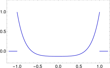
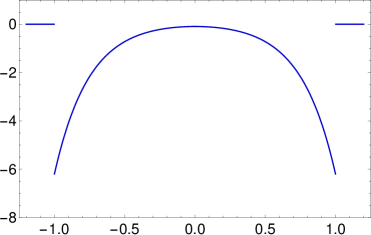
Figure 1: Plots of the three-dimensional Bopp-Podolsky Green function for $c=1$, $\ell=0.2$: (a) $G^{\text{BP}}_{(3)}(\bm{R},\tau=1)$ for $Y=Z=0$, (b) $G^{\text{BP}}_{(3)}(\bm{R}=0,\tau)$, (c) regular part of $\partial_{\tau}G^{\text{BP}}_{(3)}(\bm{R},\tau=1)$ for $Y=Z=0$, (d) regular part of $\partial_{\tau}G^{\text{BP}}_{(3)}(\bm{R}=0,\tau)$.

Using

$$\lim_{z\to 0}\,\frac{1}{z}\,J_{1}(z)=\frac{1}{2}\,,$$ (33)

on the light cone, $c\tau=R$, the Green function (32) is discontinuous (see Fig. 1a) and reads as

$$G_{(3)}^{\rm BP}(\bm{R},\tau)\simeq\frac{c}{8\pi\ell^{2}}\,H\big{(}c\tau-R)\,.$$ (34)

Furthermore, the Green function (32) shows a decreasing oscillation (see Fig. 1b) and does not have a $\delta$-singularity unlike the Green function (30). One can say, Eq. (32) describes a wake in a plasma-like vacuum.

3.2 2D Green functions

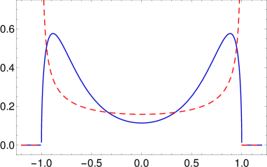
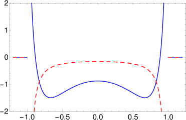
Figure 2: Plots of the two-dimensional Bopp-Podolsky Green function for $c=1$, $\ell=0.2$: (a) $G^{\text{BP}}_{(2)}(\bm{R},\tau=1)$ for $Y=0$, (b) $G^{\text{BP}}_{(2)}(\bm{R}=0,\tau)$, (c) $\partial_{\tau}G^{\text{BP}}_{(2)}(\bm{R},\tau=1)$ for $Y=0$, (d) $\partial_{\tau}G^{\text{BP}}_{(2)}(\bm{R}=0,\tau)$ (red dashed curves are the classical Green function $G_{(2)}^{\square}$ and $\partial_{\tau}G_{(2)}^{\square}$).

The two-dimensional Green functions (fundamental solutions) of the wave (d’Alembert) operator (24), the Klein-Gordon operator (25) and the Bopp-Podolsky (Klein-Gordon-d’Alembert) operator are the (generalized) functions ($\tau>0$):

$$G_{(2)}^{\square}(\bm{R},\tau) =\frac{c}{2\pi}\,\frac{H\big{(}c\tau-R\big{)}}{\sqrt{c^{2}\tau^{2}-R^{2}}}\,,$$ (35)

$$G_{(2)}^{\rm KG}(\bm{R},\tau) =\frac{c}{2\pi\ell^{2}}\,\frac{H\big{(}c\tau-R\big{)}}{\sqrt{c^{2}\tau^{2}-R^{2}}}\,\cos\bigg{(}\frac{\sqrt{c^{2}\tau^{2}-R^{2}}}{\ell}\bigg{)}\,,$$ (36)

$$G_{(2)}^{\rm BP}(\bm{R},\tau) =\frac{c}{2\pi}\,\frac{H\big{(}c\tau-R\big{)}}{\sqrt{c^{2}\tau^{2}-R^{2}}}\,\bigg{[}1-\cos\bigg{(}\frac{\sqrt{c^{2}\tau^{2}-R^{2}}}{\ell}\bigg{)}\bigg{]}\,,$$ (37)

where $R=\sqrt{(x-x^{\prime})^{2}+(y-y^{\prime})^{2}}$. Eq. (37) is obtained from Eq. (26) using the Green functions (35) and (36). The Green function (37) has been derived by Lazar [35] in the framework of dislocation gauge theory. The Green function (37) of the Bopp-Podolsky operator is zero on the light cone (see Fig. 2a), since

$$\lim_{z\to 0}\,\frac{1}{z}\,\cos(z)=\frac{1}{z}\,.$$ (38)

Furthermore, the Green function (37) shows a decreasing oscillation around the classical Green function (35) (see Fig. 2b).

3.3 1D Green functions

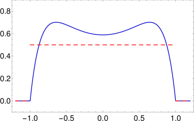
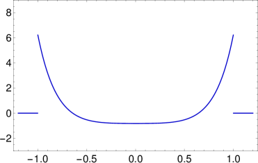
Figure 3: Plots of the one-dimensional Bopp-Podolsky Green function for $c=1$, $\ell=0.2$: (a) $G^{\text{BP}}_{(1)}(X,\tau=1)$, (b) $G^{\text{BP}}_{(1)}(X=0,\tau)$, (c) $\partial_{\tau}G^{\text{BP}}_{(1)}(X,\tau=1)$, (d) $\partial_{\tau}G^{\text{BP}}_{(1)}(X=0,\tau)$ (red dashed curves are the classical Green function $G_{(1)}^{\square}$).

The one-dimensional Green functions (fundamental solutions) of the wave (d’Alembert) operator (24), the Klein-Gordon operator (25) and the Bopp-Podolsky (Klein-Gordon-d’Alembert) operator are the (generalized) functions ($\tau>0$):

$$G_{(1)}^{\square}(X,\tau) =\frac{c}{2}\,H\big{(}c\tau-|X|)\,,$$ (39)

$$G_{(1)}^{\rm KG}(X,\tau) =\frac{c}{2\ell^{2}}\,H\big{(}c\tau-|X|\big{)}\,J_{0}\bigg{(}\frac{\sqrt{c^{2}\tau^{2}-X^{2}}}{\ell}\bigg{)}\,,$$ (40)

$$G_{(1)}^{\rm BP}(X,\tau) =\frac{c}{2}\,H\big{(}c\tau-|X|)\,\bigg{[}1-J_{0}\bigg{(}\frac{\sqrt{c^{2}\tau^{2}-X^{2}}}{\ell}\bigg{)}\bigg{]}\,,$$ (41)

where $X=x-x^{\prime}$ and $J_{0}$ is the Bessel function of the first kind of order zero. Eq. (41) is obtained from Eq. (26) using the Green functions (39) and (40). The Green function (41) of the Bopp-Podolsky operator approaches zero on the light cone (see Fig. 3a), since

$$\lim_{z\to 0}J_{0}(z)=1\,.$$ (42)

Due to the Bessel function term $J_{0}$, the Green function (41) shows a decreasing oscillation around the classical Green function (39) (see Fig. 3b).

3.4 Derivatives of the Bopp-Podolsky Green function

In this subsection, we derive the first time-derivative and first gradient of the Bopp-Podolsky Green function.

3.4.1 3D

The first time-derivative and first gradient of the three-dimensional Bopp-Podolsky Green function (32) read for $\tau>0$:

$$\partial_{\tau}G_{(3)}^{\rm BP}(\bm{R},\tau) =\frac{c^{3}\tau}{4\pi\ell^{2}}\,\bigg{[}\frac{1}{2c\tau}\,\delta\big{(}c\tau-R\big{)}-\frac{H\big{(}c\tau-R\big{)}}{(c^{2}\tau^{2}-R^{2})}\,J_{2}\bigg{(}\frac{\sqrt{c^{2}\tau^{2}-R^{2}}}{\ell}\bigg{)}\bigg{]}\,,$$ (43)

$$\nabla G_{(3)}^{\rm BP}(\bm{R},\tau) =-\frac{c\bm{R}}{4\pi\ell^{2}}\,\bigg{[}\frac{1}{2R}\,\delta\big{(}c\tau-R\big{)}-\frac{H\big{(}c\tau-R\big{)}}{(c^{2}\tau^{2}-R^{2})}\,J_{2}\bigg{(}\frac{\sqrt{c^{2}\tau^{2}-R^{2}}}{\ell}\bigg{)}\bigg{]}\,,$$ (44)

using $H^{\prime}(z)=\delta(z)$, $\delta(z)f(z)=\delta(z)f(0)$, and $(J_{1}(z)/z)^{\prime}=-J_{2}(z)/z$. $J_{2}$ is the Bessel function of the first kind of order two. Thus, Eqs. (43) and (44) consist of two terms, namely a Dirac $\delta$-term on the light cone plus a Bessel function term inside the light cone. The second parts (regular parts) of Eqs. (43) and (44) are discontinuous and show a decreasing oscillation.

On the light cone, the derivatives of the Green function $G_{(3)}^{\rm BP}$ possess a singularity of Dirac $\delta$-type. This is exhibited by the first term in Eqs. (43) and (44). The second term in Eqs. (43) and (44) is discontinuous on the light cone (see Fig. 1c), since

$$\lim_{z\to 0}\,\frac{1}{z^{2}}\,J_{2}(z)=\frac{1}{8}\,.$$ (45)

In the neighbourhood of the light cone, Eqs. (43) and (44) have the form

$$\partial_{\tau}G_{(3)}^{\rm BP}(\bm{R},\tau) \simeq\frac{c^{3}\tau}{4\pi\ell^{2}}\,\bigg{[}\frac{1}{2c\tau}\,\delta\big{(}c\tau-R\big{)}-\frac{1}{8\ell^{2}}\,H\big{(}c\tau-R\big{)}\bigg{]}\,,$$ (46)

$$\nabla G_{(3)}^{\rm BP}(\bm{R},\tau) \simeq-\frac{c\bm{R}}{4\pi\ell^{2}}\,\bigg{[}\frac{1}{2R}\,\delta\big{(}c\tau-R\big{)}-\frac{1}{8\ell^{2}}\,H\big{(}c\tau-R\big{)}\bigg{]}\,.$$ (47)

It can be seen in Fig. 1d that the second parts (regular parts) of Eqs. (43) and (44) show a decreasing oscillation.

3.4.2 2D

The first time-derivative and first gradient of the two-dimensional Bopp-Podolsky Green function (37) read for $\tau>0$:

$$\partial_{\tau}G_{(2)}^{\rm BP}(\bm{R},\tau) =-\frac{c^{3}\tau}{2\pi}\,\frac{H\big{(}c\tau-R\big{)}}{(c^{2}\tau^{2}-R^{2})^{\frac{3}{2}}}\,\bigg{[}1-\cos\bigg{(}\frac{\sqrt{c^{2}\tau^{2}-R^{2}}}{\ell}\bigg{)}-\frac{\sqrt{c^{2}\tau^{2}-R^{2}}}{\ell}\,\sin\bigg{(}\frac{\sqrt{c^{2}\tau^{2}-R^{2}}}{\ell}\bigg{)}\bigg{]}\,,$$ (48)

$$\nabla G_{(2)}^{\rm BP}(\bm{R},\tau) =\frac{c\bm{R}}{2\pi}\,\frac{H\big{(}c\tau-R\big{)}}{(c^{2}\tau^{2}-R^{2})^{\frac{3}{2}}}\,\bigg{[}1-\cos\bigg{(}\frac{\sqrt{c^{2}\tau^{2}-R^{2}}}{\ell}\bigg{)}-\frac{\sqrt{c^{2}\tau^{2}-R^{2}}}{\ell}\,\sin\bigg{(}\frac{\sqrt{c^{2}\tau^{2}-R^{2}}}{\ell}\bigg{)}\bigg{]}\,.$$ (49)

On the light cone, the derivatives of the Green function $G_{(2)}^{\rm BP}$ possess a $1/z$-singularity (see Fig. 2c), since

$$\lim_{z\to 0}\,\frac{1}{z^{3}}\,\cos(z)=\frac{1}{z^{3}}-\frac{1}{2z}$$ (50)

and

$$\lim_{z\to 0}\,\frac{1}{z^{2}}\,\sin(z)=\frac{1}{z}\,,$$ (51)

they are discontinuous. Of course, the $1/z$-singularity is weaker than the non-integrable $1/z^{3}$-singularity. In the neighbourhood of the light cone, Eqs. (48) and (49) have the form

$$\partial_{\tau}G_{(2)}^{\rm BP}(\bm{R},\tau) \simeq\frac{c^{3}\tau}{4\pi\ell^{2}}\,\frac{H\big{(}c\tau-R\big{)}}{\sqrt{c^{2}\tau^{2}-R^{2}}}\,,$$ (52)

$$\nabla G_{(2)}^{\rm BP}(\bm{R},\tau) \simeq-\frac{c\bm{R}}{4\pi\ell^{2}}\,\frac{H\big{(}c\tau-R\big{)}}{\sqrt{c^{2}\tau^{2}-R^{2}}}\,.$$ (53)

Furthermore, Eqs. (48) and (49) show a decreasing oscillation around the classical singularity (see Fig. 2d).

3.4.3 1D

The first time-derivative and space-derivative of the one-dimensional Bopp-Podolsky Green function (41) read for $\tau>0$:

$$\partial_{\tau}G_{(1)}^{\rm BP}(X,\tau) =\frac{c^{3}\tau}{2\ell}\,\frac{H\big{(}c\tau-|X|)}{\sqrt{c^{2}\tau^{2}-X^{2}}}\,J_{1}\bigg{(}\frac{\sqrt{c^{2}\tau^{2}-X^{2}}}{\ell}\bigg{)}\,,$$ (54)

$$\partial_{X}G_{(1)}^{\rm BP}(X,\tau) =-\frac{cX}{2\ell}\,\frac{H\big{(}c\tau-|X|)}{\sqrt{c^{2}\tau^{2}-X^{2}}}\,J_{1}\bigg{(}\frac{\sqrt{c^{2}\tau^{2}-X^{2}}}{\ell}\bigg{)}\,,$$ (55)

using $J_{0}^{\prime}=-J_{1}$.

On the light cone, the derivatives of the Green function $G_{(1)}^{\rm BP}$, Eqs. (54) and (55), have a jump discontinuity, due to Eq. (33) (see Fig. 3c), namely

$$\partial_{\tau}G_{(1)}^{\rm BP}(X,\tau) \simeq\frac{c^{3}\tau}{4\ell^{2}}\,H\big{(}c\tau-|X|)\,,$$ (56)

$$\partial_{X}G_{(1)}^{\rm BP}(X,\tau) \simeq-\frac{cX}{4\ell^{2}}\,H\big{(}c\tau-|X|)\,.$$ (57)

Furthermore, Eqs. (54) and (55) show a decreasing oscillation (see Fig. 3d) unlike the derivative of the Green function of the d’Alembert equation given in terms of $\delta\big{(}c\tau-|X|)$.

4 Retarded potentials and retarded electromagnetic field strengths

Solutions based on retarded Green functions lead to retarded fields (like retarded potentials and retarded electromagnetic field strengths) in the form of retarded integrals. Retarded integrals are mathematical expressions reflecting the phenomenon of “finite signal speed” (e.g. [42]).

4.1 Retarded potentials

The retarded electromagnetic potentials are the solutions of the inhomogeneous Bopp-Podolsky equations  (18) and (19) and for zero initial conditions they are given as convolution of the (retarded) Green function $G^{\rm BP}$ and the given charge and current densities ($\rho$, $\bm{J}$)

$$\phi =\frac{1}{\varepsilon_{0}}\,G^{\rm BP}*\rho\,,$$ (58)

$$\bm{A} =\mu_{0}\,G^{\rm BP}*\bm{J}\,.$$ (59)

Explicitly, the convolution integrals (58) and (59) read as

$$\phi_{(n)}(\bm{r},t) =\frac{1}{\varepsilon_{0}}\,\int_{-\infty}^{t}{\mathrm{d}}t^{\prime}\int_{\mathbb{R}^{n}}{\mathrm{d}}\bm{r}^{\prime}\,G_{(n)}^{\rm BP}(\bm{r}-\bm{r}^{\prime},t-t^{\prime})\,\rho(\bm{r}^{\prime},t^{\prime})\,,$$ (60)

$$\bm{A}_{(n)}(\bm{r},t) =\mu_{0}\int_{-\infty}^{t}{\mathrm{d}}t^{\prime}\int_{\mathbb{R}^{n}}{\mathrm{d}}\bm{r}^{\prime}\,G_{(n)}^{\rm BP}(\bm{r}-\bm{r}^{\prime},t-t^{\prime})\,\bm{J}(\bm{r}^{\prime},t^{\prime})\,,$$ (61)

where $\bm{r}^{\prime}$ is the source point and $\bm{r}$ is the field point. Here $n$ denotes the spatial dimension.

Substituting Eqs. (58) and (59) into the generalized Lorentz gauge condition (17) and using Eqs. (22) and (10), it can be seen that the generalized Lorentz gauge condition is satisfied

$$\big{[}1+\ell^{2}\square\big{]}\left(\frac{1}{c^{2}}\,\partial_{t}\phi+\nabla\cdot\bm{A}\right) =\mu_{0}\big{[}1+\ell^{2}\square\big{]}G^{\rm BP}*\big{(}\partial_{t}\rho+\nabla\cdot\bm{J}\big{)}$$

$$=\mu_{0}\big{(}\partial_{t}\rho+\nabla\cdot\bm{J}\big{)}*G^{\square}$$

$$=0\,.$$ (62)

4.1.1 3D

Substituting the Bopp-Podolsky Green function (32) into Eqs. (60) and (61), the three-dimensional retarded electromagnetic potentials read as

$$\phi_{(3)}(\bm{r},t) =\frac{c}{4\pi\varepsilon_{0}\ell}\int_{-\infty}^{t}{\mathrm{d}}t^{\prime}\int_{\mathbb{R}^{3}}{\mathrm{d}}\bm{r}^{\prime}\,\frac{H\big{(}c\tau-R\big{)}}{\sqrt{c^{2}\tau^{2}-R^{2}}}\,J_{1}\bigg{(}\frac{\sqrt{c^{2}\tau^{2}-R^{2}}}{\ell}\bigg{)}\rho(\bm{r}^{\prime},t^{\prime})$$

$$=\frac{c}{4\pi\varepsilon_{0}\ell}\int_{-\infty}^{t-R/c}{\mathrm{d}}t^{\prime}\int_{\mathbb{R}^{3}}{\mathrm{d}}\bm{r}^{\prime}\,\frac{\rho(\bm{r}^{\prime},t^{\prime})}{\sqrt{c^{2}\tau^{2}-R^{2}}}\,J_{1}\bigg{(}\frac{\sqrt{c^{2}\tau^{2}-R^{2}}}{\ell}\bigg{)}$$ (63)

and

$$\bm{A}_{(3)}(\bm{r},t) =\frac{\mu_{0}c}{4\pi\ell}\int_{-\infty}^{t}{\mathrm{d}}t^{\prime}\int_{\mathbb{R}^{3}}{\mathrm{d}}\bm{r}^{\prime}\,\frac{H\big{(}c\tau-R\big{)}}{\sqrt{c^{2}\tau^{2}-R^{2}}}\,J_{1}\bigg{(}\frac{\sqrt{c^{2}\tau^{2}-R^{2}}}{\ell}\bigg{)}\bm{J}(\bm{r}^{\prime},t^{\prime})$$

$$=\frac{\mu_{0}c}{4\pi\ell}\int_{-\infty}^{t-R/c}{\mathrm{d}}t^{\prime}\int_{\mathbb{R}^{3}}{\mathrm{d}}\bm{r}^{\prime}\,\frac{\bm{J}(\bm{r}^{\prime},t^{\prime})}{\sqrt{c^{2}\tau^{2}-R^{2}}}\,J_{1}\bigg{(}\frac{\sqrt{c^{2}\tau^{2}-R^{2}}}{\ell}\bigg{)}$$ (64)

since $H(c\tau-R)=0$ for $t^{\prime}>t-R/c$. In the Bopp-Podolsky electrodynamics, the three-dimensional retarded potentials (4.1.1) and (4.1.1) possess an afterglow, since they draw contribution emitted at all times $t^{\prime}$ from $-\infty$ up to $t-R/c$. The retarded time is a result of the finite speed of propagation for electromagnetic signals.

4.1.2 2D

Substituting the Bopp-Podolsky Green function (37) into Eqs. (60) and (61), the two-dimensional retarded electromagnetic potentials become

$$\phi_{(2)}(\bm{r},t) =\frac{c}{2\pi\varepsilon_{0}}\int_{-\infty}^{t}{\mathrm{d}}t^{\prime}\int_{\mathbb{R}^{2}}{\mathrm{d}}\bm{r}^{\prime}\,\frac{H\big{(}c\tau-R\big{)}}{\sqrt{c^{2}\tau^{2}-R^{2}}}\,\bigg{[}1-\cos\bigg{(}\frac{\sqrt{c^{2}\tau^{2}-R^{2}}}{\ell}\bigg{)}\bigg{]}\rho(\bm{r}^{\prime},t^{\prime})$$

$$=\frac{c}{2\pi\varepsilon_{0}}\int_{-\infty}^{t-R/c}{\mathrm{d}}t^{\prime}\int_{\mathbb{R}^{2}}{\mathrm{d}}\bm{r}^{\prime}\,\frac{\rho(\bm{r}^{\prime},t^{\prime})}{\sqrt{c^{2}\tau^{2}-R^{2}}}\,\bigg{[}1-\cos\bigg{(}\frac{\sqrt{c^{2}\tau^{2}-R^{2}}}{\ell}\bigg{)}\bigg{]}$$ (65)

and

$$\bm{A}_{(2)}(\bm{r},t) =\frac{\mu_{0}c}{2\pi}\int_{-\infty}^{t}{\mathrm{d}}t^{\prime}\int_{\mathbb{R}^{2}}{\mathrm{d}}\bm{r}^{\prime}\,\frac{H\big{(}c\tau-R\big{)}}{\sqrt{c^{2}\tau^{2}-R^{2}}}\,\bigg{[}1-\cos\bigg{(}\frac{\sqrt{c^{2}\tau^{2}-R^{2}}}{\ell}\bigg{)}\bigg{]}\bm{J}(\bm{r}^{\prime},t^{\prime})$$

$$=\frac{\mu_{0}c}{2\pi}\int_{-\infty}^{t-R/c}{\mathrm{d}}t^{\prime}\int_{\mathbb{R}^{2}}{\mathrm{d}}\bm{r}^{\prime}\,\frac{\bm{J}(\bm{r}^{\prime},t^{\prime})}{\sqrt{c^{2}\tau^{2}-R^{2}}}\,\bigg{[}1-\cos\bigg{(}\frac{\sqrt{c^{2}\tau^{2}-R^{2}}}{\ell}\bigg{)}\bigg{]}$$ (66)

since $H(c\tau-R)=0$ for $t^{\prime}>t-R/c$. Thus, the two-dimensional retarded potentials (4.1.2) and (4.1.2) show an afterglow, since they draw contribution emitted at all times $t^{\prime}$ from $-\infty$ up to $t-R/c$.

4.1.3 1D

In the version of the Bopp-Podolsky electrodynamics in one spatial dimension, the potentials $\phi_{(1)}$ and $A_{(1)}$ are both a scalar field, and the current density $J$ is also a scalar field.

Substituting the Bopp-Podolsky Green function (41) into Eqs. (60) and (61), the one-dimensional retarded electromagnetic potentials read

$$\phi_{(1)}(x,t) =\frac{c}{2\varepsilon_{0}}\int_{-\infty}^{t}{\mathrm{d}}t^{\prime}\int_{-\infty}^{\infty}{\mathrm{d}}x^{\prime}\,H\big{(}c\tau-|X|)\,\bigg{[}1-J_{0}\bigg{(}\frac{\sqrt{c^{2}\tau^{2}-X^{2}}}{\ell}\bigg{)}\bigg{]}\rho(x^{\prime},t^{\prime})\,$$

$$=\frac{c}{2\varepsilon_{0}}\int_{-\infty}^{t-|X|/c}{\mathrm{d}}t^{\prime}\int_{-\infty}^{\infty}{\mathrm{d}}x^{\prime}\,\rho(x^{\prime},t^{\prime})\bigg{[}1-J_{0}\bigg{(}\frac{\sqrt{c^{2}\tau^{2}-X^{2}}}{\ell}\bigg{)}\bigg{]}$$ (67)

and

$$A_{(1)}(x,t) =\frac{\mu_{0}c}{2}\int_{-\infty}^{t}{\mathrm{d}}t^{\prime}\int_{-\infty}^{\infty}{\mathrm{d}}x^{\prime}\,H\big{(}c\tau-|X|)\,\bigg{[}1-J_{0}\bigg{(}\frac{\sqrt{c^{2}\tau^{2}-X^{2}}}{\ell}\bigg{)}\bigg{]}J(x^{\prime},t^{\prime})\,$$

$$=\frac{\mu_{0}c}{2}\int_{-\infty}^{t-|X|/c}{\mathrm{d}}t^{\prime}\int_{-\infty}^{\infty}{\mathrm{d}}x^{\prime}\,J(x^{\prime},t^{\prime})\bigg{[}1-J_{0}\bigg{(}\frac{\sqrt{c^{2}\tau^{2}-X^{2}}}{\ell}\bigg{)}\bigg{]}$$ (68)

since $H(c\tau-|X|)=0$ for $t^{\prime}>t-|X|/c$. It can be seen that the one-dimensional retarded potentials (4.1.3) and (4.1.3) draw contribution emitted at all times $t^{\prime}$ from $-\infty$ up to $t-|X|/c$.

In the Bopp-Podolsky electrodynamics, the retarded potentials possess an afterglow in 1D, 2D and 3D since they draw contribution emitted at all times $t^{\prime}$ from $-\infty$ up to $t-R/c$ unlike in the classical Maxwell electrodynamics where only the retarded potentials possess an afterglow in 1D and 2D (see, e.g., [36, 38]).

4.2 Retarded electromagnetic field strengths

Substituting Eqs. (58) and (59) into the electromagnetic fields (3) and (4) or solving Eqs. (15) and (16), the electromagnetic fields ($\bm{E}$, $\bm{B}$) are given by the convolution of the Green function $G^{\rm BP}$ and the given charge and current densities ($\rho$, $\bm{J}$) and read as

$$\bm{E}_{(n)}(\bm{r},t) =-\frac{1}{\varepsilon_{0}}\,\int_{-\infty}^{t}{\mathrm{d}}t^{\prime}\int_{\mathbb{R}^{n}}{\mathrm{d}}\bm{r}^{\prime}\,\Big{(}\nabla G_{(n)}^{\rm BP}(\bm{r}-\bm{r}^{\prime},t-t^{\prime})\,\rho(\bm{r}^{\prime},t^{\prime})$$

$$\qquad\qquad\qquad\qquad+\frac{1}{c^{2}}\partial_{t}G_{(n)}^{\rm BP}(\bm{r}-\bm{r}^{\prime},t-t^{\prime})\,\bm{J}(\bm{r}^{\prime},t^{\prime})\Big{)}\,,$$ (69)

$$\bm{B}_{(n)}(\bm{r},t) =\mu_{0}\int_{-\infty}^{t}{\mathrm{d}}t^{\prime}\int_{\mathbb{R}^{n}}{\mathrm{d}}\bm{r}^{\prime}\,\nabla G_{(n)}^{\rm BP}(\bm{r}-\bm{r}^{\prime},t-t^{\prime})\times\bm{J}(\bm{r}^{\prime},t^{\prime})\,.$$ (70)

4.2.1 3D

Substituting the derivatives of the Bopp-Podolsky Green function (43) and (44) into Eqs. (4.2) and (70), the three-dimensional retarded electromagnetic field strengths read as

$$\bm{E}_{(3)}(\bm{r},t) =\frac{1}{8\pi\varepsilon_{0}\ell^{2}}\,\int_{\mathbb{R}^{3}}{\mathrm{d}}\bm{r}^{\prime}\,\bigg{(}\frac{\bm{R}}{R}\,\rho\big{(}\bm{r}^{\prime},t-R/c\big{)}-\frac{1}{c}\,\bm{J}\big{(}\bm{r}^{\prime},t-R/c\big{)}\bigg{)}$$

$$\quad-\frac{c}{4\pi\varepsilon_{0}\ell^{2}}\,\int_{-\infty}^{t-R/c}{\mathrm{d}}t^{\prime}\int_{\mathbb{R}^{3}}{\mathrm{d}}\bm{r}^{\prime}\,\frac{\big{[}\bm{R}\rho(\bm{r}^{\prime},t^{\prime})-\tau\bm{J}(\bm{r}^{\prime},t^{\prime})\big{]}}{(c^{2}\tau^{2}-R^{2})}\,J_{2}\bigg{(}\frac{\sqrt{c^{2}\tau^{2}-R^{2}}}{\ell}\bigg{)}$$ (71)

and

$$\bm{B}_{(3)}(\bm{r},t) =-\frac{\mu_{0}}{8\pi\ell^{2}}\,\int_{\mathbb{R}^{3}}{\mathrm{d}}\bm{r}^{\prime}\,\frac{\bm{R}}{R}\times\bm{J}\big{(}\bm{r}^{\prime},t-R/c\big{)}$$

$$\quad+\frac{\mu_{0}c}{4\pi\ell^{2}}\,\int_{-\infty}^{t-R/c}{\mathrm{d}}t^{\prime}\int_{\mathbb{R}^{3}}{\mathrm{d}}\bm{r}^{\prime}\,\frac{\bm{R}\times\bm{J}(\bm{r}^{\prime},t^{\prime})}{(c^{2}\tau^{2}-R^{2})}\,J_{2}\bigg{(}\frac{\sqrt{c^{2}\tau^{2}-R^{2}}}{\ell}\bigg{)}\,.$$ (72)

In the first part of Eqs. (4.2.1) and (4.2.1), the $\delta$-function in Eqs. (43) and (44) picked out the value of $\rho$ and $\bm{J}$ at the retarded time, $t-R/c$, which is earlier than $t$ by as long as it takes a signal with speed $c$ to travel from the source point ${\bm{r}}^{\prime}$ to the field point ${\bm{r}}$. From each point ${\bm{r}}^{\prime}$, the first part of Eqs. (4.2.1) and (4.2.1) draws contributions emitted at the retarded time $t-R/c$. The second part of Eqs. (4.2.1) and (4.2.1) is due to the discontinuous part of Eqs. (43) and (44) and they draw contribution emitted at all times $t^{\prime}$ from $-\infty$ up to $t-R/c$.

It can be seen that Eqs. (4.2.1) and (4.2.1) have some similarities but also differences to the so-called Jefimenko equations in Maxwell’s electrodynamics [42] (see also [43]). The differences are based on the appearance of the Bopp-Podolsky Green function (32) in the Bopp-Podolsky electrodynamics instead of the Green function of the d’Alembert operator (30) in the Maxwell electrodynamics.

4.2.2 2D

In two-dimensional electrodynamics, the magnetic field strength is a scalar field $B_{(2)}=\nabla\times\bm{A}_{(2)}=\epsilon_{ij}\partial_{i}A_{j}$, where $\epsilon_{ij}$ is the two-dimensional Levi-Civita tensor, and the electric field strength $E_{(2)}=(E_{x},E_{y})$ is a two-dimensional vector field (see, e.g., [44]).

Substituting the derivatives of the Bopp-Podolsky Green function (48) and (49) into Eqs. (4.2) and (70), the two-dimensional retarded electromagnetic field strengths become

$$\bm{E}_{(2)}(\bm{r},t) =-\frac{c}{2\pi\varepsilon_{0}}\int_{-\infty}^{t-R/c}{\mathrm{d}}t^{\prime}\int_{\mathbb{R}^{2}}{\mathrm{d}}\bm{r}^{\prime}\,\frac{\big{[}\bm{R}\rho(\bm{r}^{\prime},t^{\prime})-\tau\bm{J}(\bm{r}^{\prime},t^{\prime})\big{]}}{(c^{2}\tau^{2}-R^{2})^{\frac{3}{2}}}\,\bigg{[}1-\cos\bigg{(}\frac{\sqrt{c^{2}\tau^{2}-R^{2}}}{\ell}\bigg{)}$$

$$\qquad-\frac{\sqrt{c^{2}\tau^{2}-R^{2}}}{\ell}\,\sin\bigg{(}\frac{\sqrt{c^{2}\tau^{2}-R^{2}}}{\ell}\bigg{)}\bigg{]}$$ (73)

and

$$B_{(2)}(\bm{r},t) =\frac{\mu_{0}c}{2\pi}\int_{-\infty}^{t-R/c}{\mathrm{d}}t^{\prime}\int_{\mathbb{R}^{2}}{\mathrm{d}}\bm{r}^{\prime}\,\frac{\bm{R}\times\bm{J}(\bm{r}^{\prime},t^{\prime})}{(c^{2}\tau^{2}-R^{2})^{\frac{3}{2}}}\,\bigg{[}1-\cos\bigg{(}\frac{\sqrt{c^{2}\tau^{2}-R^{2}}}{\ell}\bigg{)}$$

$$\qquad-\frac{\sqrt{c^{2}\tau^{2}-R^{2}}}{\ell}\,\sin\bigg{(}\frac{\sqrt{c^{2}\tau^{2}-R^{2}}}{\ell}\bigg{)}\bigg{]}\,,$$ (74)

where $\bm{R}\times\bm{J}=\epsilon_{ij}R_{i}J_{j}$. The two-dimensional retarded electromagnetic field strengths (4.2.2) and (4.2.2) show an afterglow, since they draw contribution emitted at all times $t^{\prime}$ from $-\infty$ up to $t-R/c$.

4.2.3 1D

This version of the Bopp-Podolsky electrodynamics in one spatial dimension has a scalar electric field and no magnetic field (see, e.g., [45] for classical electrodynamics in one spatial dimension).

Substituting the derivatives of the Bopp-Podolsky Green function (54) and (55) into Eqs. (4.2) and (70), the one-dimensional retarded electromagnetic field strengths read as

$$E_{(1)}(x,t) =\frac{c}{2\varepsilon_{0}\ell}\int_{-\infty}^{t-|X|/c}{\mathrm{d}}t^{\prime}\int_{-\infty}^{\infty}{\mathrm{d}}x^{\prime}\,\frac{\big{[}X\rho(x^{\prime},t^{\prime})-\tau J(x^{\prime},t^{\prime})\big{]}}{\sqrt{c^{2}\tau^{2}-X^{2}}}\,J_{1}\bigg{(}\frac{\sqrt{c^{2}\tau^{2}-X^{2}}}{\ell}\bigg{)}\,,$$ (75)

$$B_{(1)}(x,t) =0\,.$$ (76)

The one-dimensional retarded electric field strength (75) possesses an afterglow, because it draws contribution emitted at all times $t^{\prime}$ from $-\infty$ up to $t-|X|/c$.

5 Generalized Liénard-Wiechert fields: electromagnetic fields of a non-uniformly moving point charge

We consider a non-uniformly moving point charge carrying the charge $q$ at the position $\bm{s}(t)$. The electric charge density and the electric current density vector are given by

$$\rho({\bm{r}},t) =q\,\delta({\bm{r}}-\bm{s}(t))\,,\qquad{\bm{J}}({\bm{r}},t)=q{\bm{V}}(t)\,\delta({\bm{r}}-\bm{s}(t))\,,$$ (77)

where ${\bm{V}}(t)=\partial_{t}{\bm{s}}(t)=\dot{\bm{s}}(t)$ is the arbitrary velocity of the non-uniformly moving point charge. We consider the case that the velocity of the point charge is less than the speed of light: $|{\bm{V}}|<c$. Therefore, the retarded potentials for non-uniformly moving point charges lead to the generalized Liénard-Wiechert potentials in the framework of Bopp-Podolsky electrodynamics.

5.1 Generalized Liénard-Wiechert potentials

5.1.1 3D

Substituting Eq. (77) into Eqs. (4.1.1) and (4.1.1) and performing the spatial integration, the three-dimensional generalized Liénard-Wiechert potentials read as

$$\phi_{(3)}(\bm{r},t) =\frac{qc}{4\pi\varepsilon_{0}\ell}\int_{-\infty}^{t_{\text{R}}}{\mathrm{d}}t^{\prime}\,\frac{1}{\sqrt{c^{2}\tau^{2}-R^{2}(t^{\prime})}}\,J_{1}\bigg{(}\frac{\sqrt{c^{2}\tau^{2}-R^{2}(t^{\prime})}}{\ell}\bigg{)}$$ (78)

and

$$\bm{A}_{(3)}(\bm{r},t) =\frac{\mu_{0}qc}{4\pi\ell}\int_{-\infty}^{t_{\text{R}}}{\mathrm{d}}t^{\prime}\,\frac{\bm{V}(t^{\prime})}{\sqrt{c^{2}\tau^{2}-R^{2}(t^{\prime})}}\,J_{1}\bigg{(}\frac{\sqrt{c^{2}\tau^{2}-R^{2}(t^{\prime})}}{\ell}\bigg{)}\,,$$ (79)

where $\bm{R}(t^{\prime})=\bm{r}-\bm{s}(t^{\prime})$ and the retarded time ${t_{\text{R}}}$ being the root of the equation

$$\big{[}x-s_{x}({t_{\text{R}}})\big{]}^{2}+\big{[}y-s_{y}({t_{\text{R}}})\big{]}^{2}+\big{[}z-s_{z}({t_{\text{R}}})\big{]}^{2}-c^{2}(t-{t_{\text{R}}})^{2}=0\,.$$ (80)

Due to the condition $|{\bm{V}}|<c$, there is only one solution of Eq. (80) which is the retarded time ${t_{\text{R}}}$. The three-dimensional generalized Liénard-Wiechert potentials (78) and (79) draw contributions emitted at all times $t^{\prime}$ from $-\infty$ up to ${t_{\text{R}}}$. The generalized Liénard-Wiechert potentials (78) and (79) are in agreement with the expressions given by Landé and Thomas [29].

5.1.2 2D

Substituting Eq. (77) into Eqs. (4.1.2) and (4.1.2) and performing the spatial integration, the two-dimensional generalized Liénard-Wiechert potentials become

$$\phi_{(2)}(\bm{r},t) =\frac{qc}{2\pi\varepsilon_{0}}\int_{-\infty}^{t_{\text{R}}}{\mathrm{d}}t^{\prime}\,\frac{1}{\sqrt{c^{2}\tau^{2}-R^{2}(t^{\prime})}}\,\bigg{[}1-\cos\bigg{(}\frac{\sqrt{c^{2}\tau^{2}-R^{2}(t^{\prime})}}{\ell}\bigg{)}\bigg{]}$$ (81)

and

$$\bm{A}_{(2)}(\bm{r},t) =\frac{\mu_{0}qc}{2\pi}\int_{-\infty}^{t_{\text{R}}}{\mathrm{d}}t^{\prime}\,\frac{\bm{V}(t^{\prime})}{\sqrt{c^{2}\tau^{2}-R^{2}(t^{\prime})}}\,\bigg{[}1-\cos\bigg{(}\frac{\sqrt{c^{2}\tau^{2}-R^{2}(t^{\prime})}}{\ell}\bigg{)}\bigg{]}\,,$$ (82)

where $\bm{R}(t^{\prime})=\bm{r}-\bm{s}(t^{\prime})$ and the retarded time ${t_{\text{R}}}$ being the root of the equation

$$\big{[}x-s_{x}({t_{\text{R}}})\big{]}^{2}+\big{[}y-s_{y}({t_{\text{R}}})\big{]}^{2}-c^{2}(t-{t_{\text{R}}})^{2}=0\,.$$ (83)

It can be seen that the two-dimensional generalized Liénard-Wiechert potentials (81) and (82) draw contributions emitted at all times $t^{\prime}$ from $-\infty$ up to ${t_{\text{R}}}$.

5.1.3 1D

Substituting Eq. (77) into Eqs. (4.1.3) and (4.1.3), the spatial integration can be performed to give the one-dimensional generalized Liénard-Wiechert potentials

$$\phi_{(1)}(x,t) =\frac{qc}{2\varepsilon_{0}}\int_{-\infty}^{t_{\text{R}}}{\mathrm{d}}t^{\prime}\,\bigg{[}1-J_{0}\bigg{(}\frac{\sqrt{c^{2}\tau^{2}-X^{2}(t^{\prime})}}{\ell}\bigg{)}\bigg{]}$$ (84)

and

$$A_{(1)}(x,t) =\frac{\mu_{0}qc}{2}\int_{-\infty}^{t_{\text{R}}}{\mathrm{d}}t^{\prime}\,V(t^{\prime})\bigg{[}1-J_{0}\bigg{(}\frac{\sqrt{c^{2}\tau^{2}-X^{2}(t^{\prime})}}{\ell}\bigg{)}\bigg{]}\,,$$ (85)

where $X(t^{\prime})=x-s(t^{\prime})$ and ${t_{\text{R}}}$ is the retarded time, which is the root of the equation

$$\big{[}x-s({t_{\text{R}}})\big{]}^{2}-c^{2}(t-{t_{\text{R}}})^{2}=0\,.$$ (86)

Also the one-dimensional generalized Liénard-Wiechert potentials (84) and (85) draw contributions emitted at all times $t^{\prime}$ from $-\infty$ up to ${t_{\text{R}}}$.

Like the retarded potentials in the Bopp-Podolsky electrodynamics, the generalized Liénard-Wiechert potentials in 3D, 2D and 1D, Eqs. (78), (79), (81), (82) and (84), (85) depend on the entire history of the point charge up to the retarded time ${t_{\text{R}}}$ and contain “tail terms”.

5.2 Generalized Liénard-Wiechert form of the electromagnetic field strengths

5.2.1 3D

Substituting Eq. (77) into Eqs. (4.2.1) and (4.2.1) and performing the spatial integration (see, e.g., [46, 47, 43]), the three-dimensional electromagnetic fields in the generalized Liénard-Wiechert form read as

$$\bm{E}_{(3)}(\bm{r},t) =\frac{q}{8\pi\varepsilon_{0}\ell^{2}}\,\bigg{[}\frac{\bm{R}(t^{\prime})}{P(t^{\prime})}-\frac{\bm{V}(t^{\prime})R(t^{\prime})}{cP(t^{\prime})}\bigg{]}_{t^{\prime}={t_{\text{R}}}}$$

$$\quad-\frac{qc}{4\pi\varepsilon_{0}\ell^{2}}\,\int_{-\infty}^{t_{\text{R}}}{\mathrm{d}}t^{\prime}\,\frac{\bm{R}(t^{\prime})-\tau\bm{V}(t^{\prime})}{(c^{2}\tau^{2}-R^{2}(t^{\prime}))}\,J_{2}\bigg{(}\frac{\sqrt{c^{2}\tau^{2}-R^{2}(t^{\prime})}}{\ell}\bigg{)}$$ (87)

and

$$\bm{B}_{(3)}(\bm{r},t) =-\frac{\mu_{0}q}{8\pi\ell^{2}}\,\bigg{[}\frac{\bm{R}(t^{\prime})\times\bm{V}(t^{\prime})}{P(t^{\prime})}\bigg{]}_{t^{\prime}={t_{\text{R}}}}$$

$$\quad+\frac{\mu_{0}qc}{4\pi\ell^{2}}\,\int_{-\infty}^{t_{\text{R}}}{\mathrm{d}}t^{\prime}\,\frac{\bm{R}(t^{\prime})\times\bm{V}(t^{\prime})}{(c^{2}\tau^{2}-R^{2}(t^{\prime}))}\,J_{2}\bigg{(}\frac{\sqrt{c^{2}\tau^{2}-R^{2}(t^{\prime})}}{\ell}\bigg{)}\,,$$ (88)

where

$$P(t^{\prime})=R(t^{\prime})-{\bm{V}}(t^{\prime})\cdot{\bm{R}}(t^{\prime})/c\,.$$ (89)

In the first part of Eqs. (5.2.1) and (5.2.1), the expression inside the brackets has to be taken at the retarded time $t^{\prime}={t_{\text{R}}}$, which is the unique solution of Eq. (80). The second part of Eqs. (5.2.1) and (5.2.1) draws contribution emitted at all times $t^{\prime}$ from $-\infty$ up to the retarded time ${t_{\text{R}}}$. Note that the term $\bm{R}(t^{\prime})/P(t^{\prime})$ in the first part of Eqs. (5.2.1) and (5.2.1) possesses a (directional) discontinuity (see also [14]).

5.2.2 2D

Substituting Eq. (77) into Eqs. (4.2.2) and (4.2.2) and performing the spatial integration, the two-dimensional electromagnetic fields in the generalized Liénard-Wiechert form become

$$\bm{E}_{(2)}(\bm{r},t) =-\frac{qc}{2\pi\varepsilon_{0}}\int_{-\infty}^{t_{\text{R}}}{\mathrm{d}}t^{\prime}\,\frac{\bm{R}(t^{\prime})-\tau\bm{V}(t^{\prime})}{(c^{2}\tau^{2}-R^{2}(t^{\prime}))^{\frac{3}{2}}}\,\bigg{[}1-\cos\bigg{(}\frac{\sqrt{c^{2}\tau^{2}-R^{2}(t^{\prime})}}{\ell}\bigg{)}$$

$$\qquad\qquad-\frac{\sqrt{c^{2}\tau^{2}-R^{2}(t^{\prime})}}{\ell}\,\sin\bigg{(}\frac{\sqrt{c^{2}\tau^{2}-R^{2}(t^{\prime})}}{\ell}\bigg{)}\bigg{]}$$ (90)

and

$$B_{(2)}(\bm{r},t) =\frac{\mu_{0}qc}{2\pi}\int_{-\infty}^{t_{\text{R}}}{\mathrm{d}}t^{\prime}\,\frac{\bm{R}(t^{\prime})\times\bm{V}(t^{\prime})}{(c^{2}\tau^{2}-R^{2}(t^{\prime}))^{\frac{3}{2}}}\,\bigg{[}1-\cos\bigg{(}\frac{\sqrt{c^{2}\tau^{2}-R^{2}(t^{\prime})}}{\ell}\bigg{)}$$

$$\qquad\qquad-\frac{\sqrt{c^{2}\tau^{2}-R^{2}(t^{\prime})}}{\ell}\,\sin\bigg{(}\frac{\sqrt{c^{2}\tau^{2}-R^{2}(t^{\prime})}}{\ell}\bigg{)}\bigg{]}\,.$$ (91)

It can be seen that the two-dimensional electromagnetic fields (5.2.2) and (5.2.2) draw contributions emitted at all times $t^{\prime}$ from $-\infty$ up to ${t_{\text{R}}}$, being the unique solution of Eq. (83).

5.2.3 1D

Substituting Eq. (77) into Eqs. (75) and (76), the spatial integration can be performed to give the one-dimensional electromagnetic fields in the generalized Liénard-Wiechert form

$$E_{(1)}(x,t) =\frac{qc}{2\varepsilon_{0}\ell}\int_{-\infty}^{t_{\text{R}}}{\mathrm{d}}t^{\prime}\,\frac{X(t^{\prime})-\tau V(t^{\prime})}{\sqrt{c^{2}\tau^{2}-X^{2}(t^{\prime})}}\,J_{1}\bigg{(}\frac{\sqrt{c^{2}\tau^{2}-X^{2}(t^{\prime})}}{\ell}\bigg{)}\,,$$ (92)

$$B_{(1)}(x,t) =0\,.$$ (93)

Thus, the one-dimensional electric field (92) draws contributions emitted at all times $t^{\prime}$ from $-\infty$ up to ${t_{\text{R}}}$, which is the unique solution of Eq. (86).

6 Conclusion

Table 1: Behaviour of the Green function of the Bopp-Podolsky electrodynamics and its first derivatives on the light cone.

Spatial dimension	Green function $G^{\text{BP}}$	First derivatives of $G^{\text{BP}}$
3D	finite and discontinuous	singular and discontinuous
2D	approaching zero	singular and discontinuous
1D	approaching zero	finite and discontinuous

We have investigated the Bopp-Podolsky electrodynamics as prototype of a dynamical gradient theory with weak nonlocality in space and time. The retarded potentials, retarded electromagnetic field strengths, generalized Liénard-Wiechert potentials and electromagnetic field strengths in generalized Liénard-Wiechert form have been calculated for 3D, 2D and 1D and they depend on the entire history from $-\infty$ up to the retarded time ${t_{\text{R}}}$. The Bopp-Podolsky field is a superposition of the Maxwell field describing a massless photon and the Klein-Gordon field describing a massive one. In particular, the Klein-Gordon part of the Bopp-Podolsky field gives rise to a decreasing oscillation around the classical Maxwell field. The Green function of the Bopp-Podolsky electrodynamics and its first derivatives have been calculated and studied in the neighbourhood of the light cone (see table 1). It turned out that the Bopp-Podolsky Green function is the regularization of the Green function of the d’Alembert operator:

$$G^{\text{BP}}=\text{reg}\,\big{[}G^{\square}\big{]}\,,$$ (94)

corresponding to the simplest case of the Pauli-Villars regularization with a single “auxiliary mass” proportional to $1/\ell$. The Green function of the Klein-Gordon operator plays the mathematical role of the regularization function in the Bopp-Podolsky electrodynamics. Moreover, the retarded Bopp-Podolsky Green function and its first derivatives show decreasing oscillations inside the forward light cone. The behaviour of the electromagnetic potentials and electromagnetic field strengths on the light cone is obtained from the behaviour of the Green function and its first derivatives in the neighbourhood of the light cone. Only in 1D the electric field strength of the Bopp-Podolsky electrodynamics is singularity-free on the light cone. In 2D and 3D, the electromagnetic field strengths in the Bopp-Podolsky electrodynamics possess weaker singularities than the classical singularities of the electromagnetic field strengths in the Maxwell electrodynamics. In order to regularize the 2D and 3D electromagnetic field strengths in the Bopp-Podolsky electrodynamics towards singular-free fields on the light cone, generalized electrodynamics of higher order might be used.

References

- Bopp [1940] F. Bopp, Eine lineare Theorie des Elektrons, Ann. Phys. (Leipzig) 38 (1940) 345–384.
- Bopp [1942] F. Bopp, Eine lineare Theorie des Elektrons II, Ann. Phys. (Leipzig) 42 (1942/43) 573–608.
- Podolsky [1942] B. Podolsky, A generalized electrodynamics: part I – non-quantum, Phys. Rev. 62 (1942) 68–71.
- Podolsky and Schwed [1948] B. Podolsky, P. Schwed, Review of a generalized electrodynamics, Rev. Mod. Phys. 20 (1948) 40–50.
- Kröner and Kessel [1966] E. Kröner, D. Kessel, Zur nichtlokalen klassischen Theorie der Dielektrika, phys. stat. sol. 17 (1966) 211–220.
- Mindlin [1964] R.D. Mindlin, Micro-structure in linear elasticity, Arch. Rational. Mech. Anal. 16 (1964) 51–78.
- Maugin [1979] G.A. Maugin, Nonlocal theories or gradient-type theories: a matter of convenience? Arch. Mech. 31 (1979) 15–26.
- Eringen [2002] A.C. Eringen, Nonlocal Continuum Field Theories, Springer, New York, 2002.
- Lazar and Maugin [2005] M. Lazar, G.A. Maugin, Nonsingular stress and strain fields of dislocations and disclinations in first strain gradient elasticity, Int. J. Engng. Sci. 43 (2005) 1157–1184.
- Agiasofitou and Lazar [2009] E.K. Agiasofitou, M. Lazar, Conservation and balance laws in linear elasticity of grade three, J. Elast. 94 (2009) 69–85.
- Iwanenko and Sokolow [1953] D. Iwanenko, A. Sokolow, Klassische Feldtheorie, Akademie-Verlag, Berlin, 1953.
- Landé and Thomas [1944] A. Landé, L.H. Thomas, Finite self-energies in radiation theory. part III, Phys. Rev. 65 (1944) 175–183.
- Zayats [2014] A.E. Zayats, Self-interaction in the Bopp-Podolsky electrodynamics: Can the observable mass of a charged particle depend on its acceleration? Ann. Phys. 342 (2014) 11–20.
- Gratus et al. [2015] J. Gratus, V. Perlick, R.W. Tucker, On the self-force in Bopp-Podolsky electrodynamics, J. Phys. A: Math. Theor. 48 (2015) 435401.
- Rohrlich [1965] F. Rohrlich, Classical Charged Particles, Addison Wesley, 1965.
- Spohn [2004] H. Spohn, Dynamics of Charged Particles and Their Radiation Field, Cambridge University Press, Cambridge, 2004.
- Lazar [2014] M. Lazar, On gradient field theories: gradient magnetostatics and gradient elasticity, Phil. Mag. 94 (2014) 2840–2874.
- Frenkel [1996] F. Frenkel, problem in classical electrodynamics, Phys. Rev. E 54 (1996) 5859–5862.
- Frenkel and Santos [1999] F. Frenkel, R. Santos, On the self-force of a charged particle in classical electrodynamics, Int. J. Mod. Phys. B 13 (1999) 315–324.
- Cuzinatto et al. [2011] R.R. Cuzinatto, C.A.M. de Melo, L.G. Medeiros, P.J. Pompeia, How can one probe Podolsky electrodynamics? Int. J. Mod. Phys. A 26 (2011) 3641–3651.
- Kvasnica [1960] J. Kvasnica, A possible estimate of the elementary length in the electromagnetic interactions, Czech. J. Phys. B 10 (1960) 625–627.
- Cuzinatto et al. [2007] R.R. Cuzinatto, C.A.M. de Melo, P.J. Pompeia, Second order gauge theory, Ann. Phys. (N.Y.) 322 (2007) 1211–1232.
- Kvasnica [1960] J. Kvasnica, A remark on Bopp-Podolsky electrodynamics, Czech. J. Phys. B 10 (1960) 81–90.
- Ji et al. [2019] C.-R. Ji, A.T. Suzuki, J.H.O. Sales, R. Thibes, Pauli-Villars regularization elucidated in Bopp-Podolsky’s generalized electrodynamics, [arXiv:1902.07632].
- Santos [2011] R.B.B. Santos, Plasma-like vacuum in Podolsky regularized classical electrodynamics, Mod. Phys. Lett. A 26 (2011) 1909–1915.
- Jackson [1999] J.D. Jackson, Classical Electrodynamics, 3rd ed., Wiley, New York, 1999.
- Heald and Marion [1995] M.A. Heald, J.B. Marion, Classical Electromagnetic Radiation, 3rd ed., Brooks/Cole Thomson Learning, 1995.
- Smith [1997] G.S. Smith, An Introduction to Classical Electromagnetic Radiation, Cambridge University Press, Cambridge, 1997.
- Landé and Thomas [1941] A. Landé, L.H. Thomas, Finite self-energies in radiation theory. part II, Phys. Rev. 60 (1942) 514–23.
- Galvão and Pimentel [1988] C.A.P. Galvão, B.M. Pimentel, The canonical structure of Podolsky’ s generalized electrodynamics, Can. J. Phys. 66 (1988) 460–466.
- Bufalo et al. [2011] R. Bufalo, B.M. Pimentel, G.E.R. Zambrano, Path integral quantization of generalized quantum electrodynamics, Phys. Rev. D 83 (2011) 045007.
- Bufalo et al. [2012] R. Bufalo, B.M. Pimentel, G.E.R. Zambrano, Renormalizability of generalized quantum electrodynamics, Phys. Rev. D 86 (2012) 125023.
- Schwartz [1950/51] L. Schwartz, Théorie des Distributions, Tomes I et II, Hermann, Paris, 1950/51.
- Hörmander [1983] L. Hörmander, The Analysis of Linear Partial Differential Operators II, Springer, Berlin, 1983.
- Lazar [2010] M. Lazar, The gauge theory of dislocations: a nonuniformly moving screw dislocation, Phys. Lett. A 374 (2010) 3092–3098.
- Barton [1989] G. Barton, Elements of Green’s Functions and Propagation, Oxford University Press, Oxford, 1989.
- Kanwal [2004] R.P. Kanwal, Generalized Functions: Theory and Applications, 3rd ed., Birkhäuser, Boston, 2004.
- Vladimirov [1971] V.S. Vladimirov, Equations of Mathematical Physics, Marcel Dekker, Inc., New York, 1971.
- Zauderer [1983] E. Zauderer, Partial Differential Equations of Applied Mathematics, John Wiley & Sons Inc, New York, 1983.
- Polyanin [2001] A.D. Polyanin, Handbook of Linear Partial Differential Equations for Engineers and Scientists, Chapman and Hall/CRC, Boca Raton, 2002.
- Höhler [1951] G. Höhler, Zur Theorie der verallgemeinerten Wellengleichung, Ann. Phys. (Leipzig) 444 (1951) 77–90.
- Jefimenko [1966] O.D. Jefimenko, Electricity and Magnetism, Appleton-Century-Crofts, New York, 1966.
- Lazar [2013] M. Lazar, On retardation, radiation and Liénard-Wiechert type potentials in electrodynamics and elastodynamics, Wave Motion 50 (2013) 1161–1174.
- Lapidus [1982] I.R. Lapidus, Classical electrodynamics in a universe with two space dimensions, Am. J. Phys. 50 (1982) 155–157.
- Galić [1988] H. Galić, Fun and frustration with hydrogen in a 1+1 dimension, Am. J. Phys. 56 (1988) 312–317.
- Eyges [1972] L. Eyges, The Classical Electromagnetic Field, Addison-Wesley, Reading, MA, 1972.
- Jones [1986] D.S. Jones, Acoustic and Electromagnetic Waves, Oxford University Press, Oxford, 1986.