DropletSMOKE++: a comprehensive multiphase CFD framework for the evaporation of multidimensional fuel droplets

Abstract

This paper aims at presenting the DropletSMOKE++ solver, a comprehensive multidimensional computational framework for the evaporation of fuel droplets, under the influence of a gravity field and an external fluid flow. The Volume Of Fluid (VOF) methodology is adopted to dynamically track the interface, coupled with the solution of energy and species equations. The evaporation rate is directly evaluated based on the vapor concentration gradient at the phase boundary, with no need of semi-empirical evaporation sub-models.
The strong surface tension forces often prevent to model small droplets evaporation, because of the presence of parasitic currents. In this work we by-pass the problem, eliminating surface tension and introducing a centripetal force toward the center of the droplet. This expedient represents a major novelty of this work, which allows to numerically hang a droplet on a fiber in normal gravity conditions without modeling surface tension. Parasitic currents are completely suppressed, allowing to accurately model the evaporation process whatever the droplet size.
DropletSMOKE++ shows an excellent agreement with the experimental data in a wide range of operating conditions, for various fuels and initial droplet diameters, both in natural and forced convection. The comparison with the same cases modeled in microgravity conditions highlights the impact of an external fluid flow on the evaporation mechanism, especially at high pressures. Non-ideal thermodynamics for phase-equilibrium is included to correctly capture evaporation rates at high pressures, otherwise not well predicted by an ideal gas assumption. Finally, the presence of flow circulation in the liquid phase is discussed, as well as its influence on the internal temperature field.
DropletSMOKE++ will be released as an open-source code, open to contributions from the scientific community.

1 Introduction

The high energy density of liquid fuels is nowadays exploited in many engineering devices such as diesel engines and industrial burners. Spray injection systems are widely used in order to disperse the liquid fuel in an oxidizing environment and the control of this process is currently an active area of research. In particular, the study of a single isolated droplet allows to neglect complex interaction phenomena (coalescence, breakup, etc.) among droplets and to focus on the evaporation and combustion mechanisms. In the last decades the numerical modeling of droplets evaporation and combustion has considerably improved. Starting from the works of Spalding [spalding1953combustion] and Godsave [godsave1953studies] concerning the well known ”$d^{2}$ law”, derived under the hypothesis of a perfectly spherical, motionless and constant liquid temperature droplet, Abramzon and Sirignano [abramzon1989droplet, sirignano1999fluid] started to account for a convective flow, providing numerous correlations for the heat and mass transfer outside and within the droplet in presence of a relative gas motion. In this context, Dwyer et al. analyzed the droplet dynamics in high $T$ fields [dwyer1989calculations, dwyer1985detailed]. In particular, the transient surface heating has been investigated by Law [law1976unsteady], assuming a constant spatial liquid temperature, while Kotake and Okazaki [kotake1969evaporation] started to analyze the influence of the liquid internal circulation on the vaporization rate. More recently, Sazhin et al. analyzed the heating and evaporation process [sazhin2014modelling, sazhin2006advanced], as well as the effect of thermal radiation [abramzon2005droplet].
With the growing available computational power, the direct numerical solution of the equations governing the evolution of isolated fuel droplets became affordable, allowing the detailed 1D modeling of spherical fuel droplets in microgravity conditions [marchese1999numerical, cuoci2005autoignition, farouk2014isolated]. Microgravity conditions can be reproduced conducting the experiments in free-falling chambers [okajima1975further, kumagai1971combustion, chauveau2000effects], both for suspended and free droplets. Recently, some experiments have been conducted aboard the International Space Station (ISS) for the study of evaporation and multi-stage combustion phenomena. The absence of gravity allows to adopt a simple 1D mathematical description and to focus on physical aspects such as differential species diffusion, non-ideal thermodynamics and combustion kinetics. In particular, the implementation of detailed mechanisms for gas-phase chemistry in 1D models has paved the way for a better understanding of low-T chemistry [farouk2017combustion, farouk2017isolated, dietrich2014droplet] , ignition and extinction phenomena [cuoci2017flame, stagni2018numerical].
However, most of experiments on droplets are conducted under the influence of a gravity field, since experimental devices are much cheaper and the operating conditions are closer to the real ones where droplets are commonly adopted. 1D models are intrinsically not able to predict physical phenomena such as buoyancy, droplet deformation, relative gas motion and internal circulation, which are always present in real conditions. In particular, the external flow field (both induced and forced) around the droplet strongly modifies the evaporation rate at the interface, while the liquid circulation governs the internal heat transfer.
From the modeling point of view, the description of these phenomena requires at least a 2D multiphase model, able to predict the anisotropic deformation of the droplet and to provide both liquid and gas velocity fields. This must be coupled with a reliable evaporation model to describe the droplet shrinking, the diffusion of vapor towards the gas-phase and its further transport, both by the external convection and by the induced Stefan flow. The energy transfer between the two phases is also necessary, as well as proper correlations for the fluid properties.
Among the several methods available for multiphase flows, the Volume Of Fluid (VOF) methodology [hirt1981volume] is widely known for its simplicity, robustness and especially for the excellent mass conservation properties. Its application for evaporation and condensation phenomena has been investigated in recent years [nabil2016interthermalphasechangefoam, georgoulas2017enhanced, nieves2015openfoam, guo2014review]. However, most of these works rely on phase-change models based on experimental data, kinetic theories and semi-empirical correlations. A more general evaporation model based on the interface concentration gradient has been implemented by Shlottke [schlottke2008direct], neglecting however the detailed characterization of thermodynamic equilibrium at the interface and without a comparison of the results with experimental data. More recently, Gatha et al. [ghata2014computational, ghata2015computational] used a VOF technique to model droplet evaporation and combustion, limiting however the investigation to microgravity conditions.
A major numerical issue of VOF method concerns surface tension. Small droplets dynamics involve strong surface tension forces, which are extremely difficult to model due to the presence of the so-called parasitic currents [brackbill1992continuum]. These currents tend to numerically deform and eventually destroy the droplet, due to inaccuracies on the evaluation of the surface curvature. Some techniques [cummins2005estimating, popinet2018numerical] have been developed to mitigate parasitic currents for particular cases (e.g. rising bubbles, inviscid static droplets, capillary oscillations), but small droplets evaporation still suffers from this issue. The rapid size reduction of the droplet makes surface tension to be more and more dominant, further amplifying the problem. Even if some works concerning droplets vaporization with VOF methodology are available in literature [strotos2016predicting, banerjee2013numerical, george2017detailed], the problem of parasitic currents is often not even mentioned. These works are based on commercial CFD codes (mainly $\texttt{Ansys FLUENT}^{\textregistered}$ and $\texttt{COMSOL}^{\textregistered}$), making very difficult to reproduce the results with open-source codes since the adopted numerical algorithms are not provided in detail. Concerning the numerical framework, promising results have been reached by codes such as FS3D [eisenschmidt2016direct] and Gerris [popinet2009accurate], whereas the $\texttt{OpenFOAM}^{\textregistered}$ environment is still lacking in comprehensive solvers for the detailed analysis of droplets evaporation.
This work aims at presenting an open-source general computational tool (called DropletSMOKE++) for the modeling of isolated droplets evaporation under convective conditions in the presence of a gravity field, overcoming the aforementioned limits of the currently available solvers. In particular it includes:

• An accurate interface tracking method, based on a geometrical advection, coupled with the Navier-Stokes equations, numerically solved for both liquid and gas phase.

• A reliable evaporation model based on the surface mass flux, coupled with a species equation, with no need of semi-analytical approaches or correlations based on mass-heat transfer dimensionless numbers.

• The detailed description of the vapor-liquid equilibrium thermodynamics, including fugacity coefficients and Poynting correction calculation using a cubic Equation of State.

• A numerical technique which suppresses parasitic currents and by-passes the problem of curvature evaluation, introducing an external centripetal force to mimic surface tension effects.

The DropletSMOKE++ code is fully implemented within the open-source $\texttt{OpenFOAM}^{\textregistered}$ framework to manage the computational mesh and the discretization of governing equations. The numerical code will be freely available and open for contributions from the scientific community. The code version used for this work is provided in the supplementary material.
The paper organization includes a thorough description of the mathematical model, as well as the numerical methodology adopted. The centripetal force substituting surface tension is discussed in detail, including its numerical implementation, its effect on the droplet shape and how it impacts evaporation.
A quantitative assessment of the code has been performed, comparing the DropletSMOKE++ results with a reference finite-differences based solver for droplets evaporation in microgravity conditions [cuoci2005autoignition]. Afterwards, the gravity field has been introduced, allowing the analysis of the natural and forced convection regime.
An extensive validation with available experimental data has been carried on for n-heptane, n-decane and n-hexadecane droplets in a very wide range of operating conditions, both for natural and forced convection. Experimental data from various authors include the normalized equivalent diameter decay and some data on the surface temperature behavior, which have been compared with the DropletSMOKE++ numerical results. Equivalent numerical cases (with the same initial conditions) have been simulated also in microgravity conditions in order to highlight the main differences between the models and the intrinsic inability of microgravity solvers to correctly predict the experimental data. Finally, the presence of internal circulation in the liquid phase is briefly analyzed.

2 Mathematical model

2.1 Interface advection

The VOF methodology is often referred to as a ”one-fluid” approach, where the two phases are treated as a single fluid whose properties vary abruptly at the phase boundary. A scalar marker function $\alpha$ represents the liquid volumetric fraction, varying from value 0 in the gas-phase to value 1 in the liquid phase. The $\alpha$ advection equation in the most general form is:

$$\frac{\partial\left(\rho\alpha\right)}{\partial t}+\nabla\cdot\left(\rho\alpha\textbf{v}\right)=-\dot{m}$$ (1)

The source term $\dot{m}$ represents the evaporation/condensation contribution to the liquid. Rewriting the equation in function of $\alpha$:

$$\frac{\partial\alpha}{\partial t}+\nabla\cdot\left(\textbf{v}\alpha\right)=-\frac{\dot{m}}{\rho}-\frac{\alpha}{\rho}\frac{D\rho}{Dt}$$ (2)

This equation is solved in two steps, treating the advection and the source terms in a segregated approach, similarly to what happens in an operator-splitting technique. The interface tracking is solved first, using the isoAdvector library developed by Roenby and Jasak [roenby2016computational] :

$$\frac{\partial\alpha}{\partial t}+\nabla\cdot\left(\textbf{v}\alpha\right)=0$$ (3)

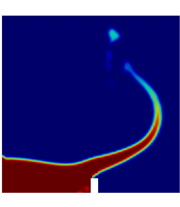
(a)

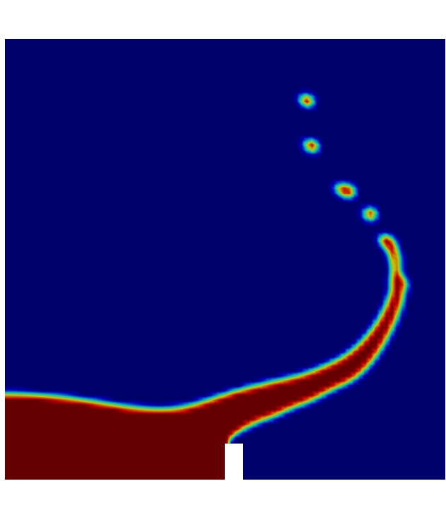
(b)

Figure 1: Comparison of the interface resolution between the MULES compressive scheme (Figure a) and isoAdvector (Figure b) for the well known damBreak case [greenshields2015openfoam].

isoAdvector performs a geometric advection of the interface, whose quality is superior (Figure 1) to the MULES (Multidimensional Universal Limiter with Explicit Solution) compressive scheme by Weller [damian2013extended] usually used in $\texttt{OpenFOAM}^{\textregistered}$ multiphase solvers. The source terms are included in a second step:

$$\frac{\partial\alpha}{\partial t}=-\frac{\dot{m}}{\rho}-\frac{\alpha}{\rho}\frac{D\rho}{Dt}$$ (4)

where the first term accounts for the evaporation, while the second term describes the liquid density variation, and eventually the droplet expansion due to external heating.

2.2 Pressure and velocity fields

A single Navier-Stokes equation is solved for both phases:

$$\frac{\partial\left(\rho\textbf{v}\right)}{\partial t}+\nabla\cdot\left(\rho\textbf{v}\otimes\textbf{v}\right)=\nabla\cdot\mu\left(\nabla\textbf{v}+\nabla\textbf{v}^{T}\right)-\nabla p+\rho\textbf{g}$$ (5)

It is convenient to separate the hydrostatic pressure $\rho\textbf{g}\cdot\textbf{r}$ from the total pressure $p$, in order to simplify the definition of boundary conditions for pressure:

$$\frac{\partial\left(\rho\textbf{v}\right)}{\partial t}+\nabla\cdot\left(\rho\textbf{v}\otimes\textbf{v}\right)=\nabla\cdot\mu\left(\nabla\textbf{v}+\nabla\textbf{v}^{T}\right)-\nabla p_{rgh}-\textbf{g}\cdot\textbf{r}\nabla\rho$$ (6)

where $p_{rgh}=p-\rho\textbf{g}\cdot\textbf{r}$ is the dynamic pressure and r is the position vector.
The continuity equation (needed for the pressure-velocity coupling) accounts for the density variations and for the abrupt change of density at the interface occurring during the evaporation, generating the Stefan flow:

$$\frac{\alpha}{\rho_{L}}\frac{D\rho_{L}}{Dt}+\frac{1-\alpha}{\rho_{G}}\frac{D\rho_{G}}{Dt}+\dot{m}\left(\frac{1}{\rho_{L}}-\frac{1}{\rho_{G}}\right)+\nabla\cdot\textbf{v}=0$$ (7)

In case of constant density and no evaporation Equation 7 reduces to the continuity equation for incompressible flows $\nabla\cdot\textbf{v}=0$.

2.3 Temperature and species fields

Additionally, energy and species equations are included:

$$\rho C_{p}\left(\frac{\partial T}{\partial t}+\textbf{v}\nabla T\right)=\nabla\cdot\left(k\nabla T\right)+\beta\frac{Dp}{Dt}-\sum_{i=0}^{Ns}\textbf{j}_{d,i}C_{p,i}\nabla T-\sum_{i=0}^{Ns_{L}}\dot{m}_{i}\Delta h_{ev,i}$$ (8)

$$\rho\left(\frac{\partial\omega_{i}}{\partial t}+\textbf{v}\nabla\omega_{i}\right)=-\nabla\cdot\textbf{j}_{d,i}$$ (9)

The last term in Equation 8 accounts for the interface cooling during evaporation. The diffusion fluxes $\textbf{j}_{d,i}$ are discussed in the next section.

2.4 Evaporation model

In this work, the mass evaporation flux is calculated based on the interface concentration gradient of the vapor. Its evaluation is not trivial, since it strongly depends on how the diffusion coefficients are computed. The species diffusion coefficients $\mathcal{D}_{i}$ in the mixture are evaluated based on the binary diffusion coefficients and the mole fractions:

$$\mathcal{D}_{i}=\frac{\sum_{j\neq i}y_{j}M_{w,j}}{M_{w}\sum_{j\neq i}\frac{y_{i}}{\mathcal{D}_{i,j}}}$$ (10)

which means that the diffusion velocities $\textbf{v}_{d,i}$ must be evaluated based on the mole fraction gradient of the species [bird2002transport]:

$$\textbf{v}_{d,i}=-\mathcal{D}_{i}\frac{\nabla y_{i}}{y_{i}}$$ (11)

The diffusion fluxes $\textbf{j}_{d,i}$ are defined as:

$$\textbf{j}_{d,i}=\rho\omega_{i}\textbf{v}_{d,i}=-\rho\omega_{i}\mathcal{D}_{i}\frac{\nabla y_{i}}{y_{i}}=-\rho\mathcal{D}_{i}\frac{M_{w,i}}{M_{w}}\nabla y_{i}$$ (12)

This expression of the diffusion flux is also used in Equation 9.

A convective flux $\textbf{j}_{c,i}$ is generated by the interfacial density change during the evaporation process, as stated in Equation 7:

$$\textbf{j}_{c,i}=\rho\omega_{i}\textbf{v}$$ (13)

The total evaporating flux $\textbf{j}_{i}$ is the sum of diffusive and convective fluxes:

$$\textbf{j}_{i}=\textbf{j}_{d,i}+\textbf{j}_{c,i}$$ (14)

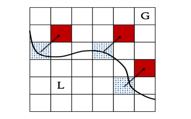
(a)

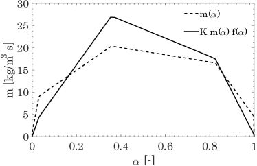
(b)

Figure 2: Calculation of $\dot{m}_{i}=\textbf{j}_{i}|\nabla\alpha|$ in Figure (a): interface cells (in dotted blue) associated to the adjacent gas-phase cells (in red). In Figure (b): evaporation flux $\dot{m}$ distribution over the interface for standard implementation (dashed line, Equation 16) and corrected implementation (solid line, Equation 19).

The local surface area per unit volume is usually computed from the $\alpha$ function as $|\nabla\alpha|$, since its volume integral is the surface area by definition:

$$S=\int_{V}|\nabla\alpha|dV$$ (15)

The evaporation rate for species $i$ is then:

$$\dot{m}_{i}=\textbf{j}_{i}\nabla\alpha$$ (16)

It is important to point out that $|\nabla\alpha|$ is calculated at the interface cells (where $|\nabla\alpha|\neq 0$), while $\textbf{j}_{i}$ must be computed at the gas cells adjacent to the interface cells. Referring to Figure 2 (a), a specific algorithm has been developed to associate every cell at the interface (represented in dotted blue) to the closest cell in the gas-phase (represented in red) along the interface normal (black arrow). Indicating with subscript $int$ a generic interface cell and with $adj$ the closest adjacent gas-phase cell with respect to $int$, we have:

$$\dot{m}_{i}|_{int}=\textbf{j}_{i}|_{adj}|\nabla\alpha|_{int}$$ (17)

which has to be evaluated for every cell at the interface.

The total evaporation rate $\dot{m}$ is the sum over the liquid (evaporating) species:

$$\dot{m}=\sum_{i=0}^{Ns_{L}}\dot{m}_{i}$$ (18)

When solving Equation 4 it is important to ensure a sharp interface. However, it is possible for $\alpha$ to reach negative values in certain cells, especially if $\dot{m}$ is high enough. In order to avoid this, $\dot{m}$ is multiplied by a proper function of $\alpha$, whose aim is to force $\dot{m}$ to be zero when $\alpha$ approaches zero. Differently from previous works [guo2014review], the evaporating flux is evaluated as follows:

$$\dot{m}=Kf(\alpha)\sum_{i=0}^{Ns_{L}}\dot{m}_{i}$$ (19)

where the constant $K$ is introduced to ensure the conservation of the integral mass flux $\int_{V}\dot{m}dV$. It is simply recovered equaling Equations 18 and 19 after a volume integration:

$$K=\frac{\int_{V}\dot{m}dV}{\int_{V}f\left(\alpha\right)\dot{m}dV}$$ (20)

We have chosen the function $f(\alpha)$ as follows:

$$f(\alpha)=\sqrt{\alpha\left(1-\alpha\right)}$$ (21)

which is a redistribution of $\dot{m}$ over the interface, as shown in Figure 2. This function goes to $0$ and to $1$ much faster, which helps to maintain a sharp interface after Equation 4 solution.

2.5 Thermodynamic equilibrium

The characterization of equilibrium thermodynamics at the phase boundary is crucial for a correct prediction of experimental data, especially for non-ideal mixtures and high pressure cases. In this work a detailed thermodynamics is included, based on Peng and Robinson equation of state [peng1976new] for the evaluation of the compressibility factor $Z$ and the fugacity coefficients $\phi_{i}$.
The vapor-liquid equilibrium relation for a two-phase systems is [smithintroduction]:

$$p_{i}^{0}(T)x_{i}\phi_{i}\left(T,p_{i}^{0}\right)e^{\int_{p_{i}^{0}}^{p}\frac{v_{L,i}}{RT}dp}=py_{i}\hat{\phi}_{i}(T,p,y_{i})$$ (22)

where $p_{i}^{0}(T)$ is the vapor pressure of species $i$, $\phi_{i}$ is the gas-phase fugacity coefficient for the pure species and $\hat{\phi}_{i}$ is the gas-phase mixture fugacity coefficient. The exponential term represents the Poynting correction, while $x_{i}$ and $y_{i}$ are the liquid and gas mole fractions of species $i$. The gaseous mole fraction $y_{i}$ is evaluated in a segregated approach, from equation 22:

$$y_{i}=\frac{p_{i}^{0}(T)\phi_{i}\left(T,p_{i}^{0}\right)e^{\int_{p_{i}^{0}}^{p}\frac{v_{L,i}}{RT}dp}}{p\hat{\phi}_{i}(T,p,y_{i})}x_{i}$$ (23)

This saturation mole fraction is assigned to the whole liquid phase and then advected in the gas phase through Equation 9, following the approach described in [banerjee2004algorithm].
The gas density is calculated by:

$$\rho_{G}=\frac{pM_{w}}{Z(T,p,y_{i})RT}$$ (24)

where $Z$ is provided by the Peng-Robinson cubic equation of state.
The molar volume $v_{L}$ in the Poynting correction is simply evaluated as:

$$v_{L,i}=\frac{M_{w,i}}{\rho_{L}}$$ (25)

2.6 The problem of surface tension: introduction of the centripetal force field

The droplet-gas interaction is characterized by high density ratios between the two phases and strong surface tension forces, particularly enhanced in small droplet sizes. Even though VOF methods are widely recognized for the great efficiencies in describing topologically complex interfaces, the accurate representation of surface tension is still a major problem in multiphase flows [popinet2018numerical].
The continuous representation of surface tension force $\textbf{f}_{s}$ by Brackbill [brackbill1992continuum] requires an accurate evaluation of the interface curvature $\kappa$:

$$\textbf{f}_{s}=\sigma\kappa\nabla\alpha$$ (26)

where curvature $\kappa$ is evaluated as:

$$\kappa=\nabla\cdot\left(\frac{\nabla\alpha}{|\nabla\alpha|}\right)$$ (27)

The $\alpha$ gradient evaluation is numerically challenging, because of the discontinuous nature of the $\alpha$ function. A direct implementation of Equation 26 creates a numerical imbalance between the surface tension force $\textbf{f}_{s}$ and the pressure gradient $\nabla p$ in the Navier-Stokes equation. As a consequence, unphysical flows and pressure spikes are generated around the interface, whose magnitude is proportional to $\sigma$ and inversely proportional to the droplet size. For the typical droplet diameters of the experiments (usually no more than 1-1.5 mm) these flows can strongly deform the interface and eventually break the droplet apart. Several methods have been proposed in this context, such as balanced force algorithms [francois2006balanced] to reduce the numerical imbalance in surface tension force evaluation, height functions [francois2006balanced] to compute the interface curvature directly from the $\alpha$ field and artificial viscosity methods [denner2017artificial]. A sophisticated combination of quad/octree spatial discretization, height functions and balanced algorithms has been implemented by Popinet [popinet2009accurate] in Gerris solver.
Concerning the $\texttt{OpenFOAM}^{\textregistered}$ environment, Albadawi [albadawi2013influence] proposed a coupled VOF-Level Set to mitigate the parasitic currents, while Raeini [raeini2012modelling] introduced smoothing factors for $\kappa$ field combined with the introduction of a capillary pressure equation and a curtailing of the $\alpha$ marker. Even if these latter methods significantly improve the modeling of surface tension forces, they have been validated on bubbles growth, stationary droplets and capillary flows, whereas no test case can be found on small droplets dynamics. Their application on the cases of our interest did not provide satisfactory results, mainly because the droplet shrinking due to the evaporation exponentially amplified the problem: the lower was the droplet size, the stronger were the parasitic currents around the interface, even if the initial stationary droplet was stabilized enough.

In this work, in order to avoid these problems, parasitic currents have been suppressed directly from their source imposing zero surface tension. In presence of a gravity field surface tension is essential to hang the droplet on a fiber or a wire. Therefore, its elimination required the introduction of an additional force to compensate the droplet weight.
A small spherical fiber is initially introduced inside the liquid droplet. A centripetal force directed toward the center of the fiber have been imposed, defined as:

$$\textbf{f}_{m}=\rho\alpha\nabla\xi$$ (28)

where $\xi$ is a scalar potential field defined as:

$$\xi=\xi_{0}\frac{D_{f}}{2r}$$ (29)

where $D_{f}$ is the fiber radius ($D_{f}=0.05$ mm in this work), $r$ is the distance from the fiber center and $\xi_{0}$ the intensity of the potential field. The $\alpha$ term in Equation 28 forces $\textbf{f}_{m}$ to be applied to the sole liquid phase and makes $\textbf{f}_{m}$ to be proportional to the droplet volume, as it is for gravity forces.
The result is a force field directed towards the droplet center and only applied to the liquid phase, similarly to what happens in a magnetic attraction of a ferrofluid. The Navier-Stokes equation becomes:

$$\frac{\partial\left(\rho\textbf{v}\right)}{\partial t}+\nabla\cdot\left(\rho\textbf{v}\otimes\textbf{v}\right)=\nabla\cdot\mu\left(\nabla\textbf{v}+\nabla\textbf{v}^{T}\right)-\nabla p_{rgh}-\textbf{g}\cdot\textbf{r}\nabla\rho+\textbf{f}_{m}$$ (30)

It is important to notice that the combination of a geometrical advection (i.e. isoAdvector) and the absence of surface tension $\sigma$ allows to track the interface maintaining a very high resolution, without any additional correction (such as filtering kernels, smoothing factors etc.) usually needed in the VOF methodology because of the strong gradients involved. The detailed numerical description and the implementation of the centripetal force $\textbf{f}_{m}$ are presented in the next section, as well as a sensitivity analysis on the value $\xi_{0}$ to be used in the simulations. The effect of the initial droplet shape on the evaporation will be also discussed.

2.7 Fluid properties

The evaluation of transport and thermodynamics properties is based on the OpenSMOKE++ library [cuoci2015opensmoke++]. Gas properties (diffusion coefficients, thermal conductivity, heat capacities and viscosity) are based on the kinetic theory of gases, while liquid properties (vapor pressure, density, conductivity, heat capacity, viscosity and vaporization heat) are evaluated based on the correlations available in the Yaws database [yaws2015yaws].
Mixture properties to be used in the governing equations can be then computed. For a generic property $\chi$:

$$\chi=\chi_{L}\alpha+\chi_{G}\left(1-\alpha\right)$$ (31)

with $\chi=\rho,\mu,C_{p},k,\mathcal{D}_{i}$.

3 Numerical methodology

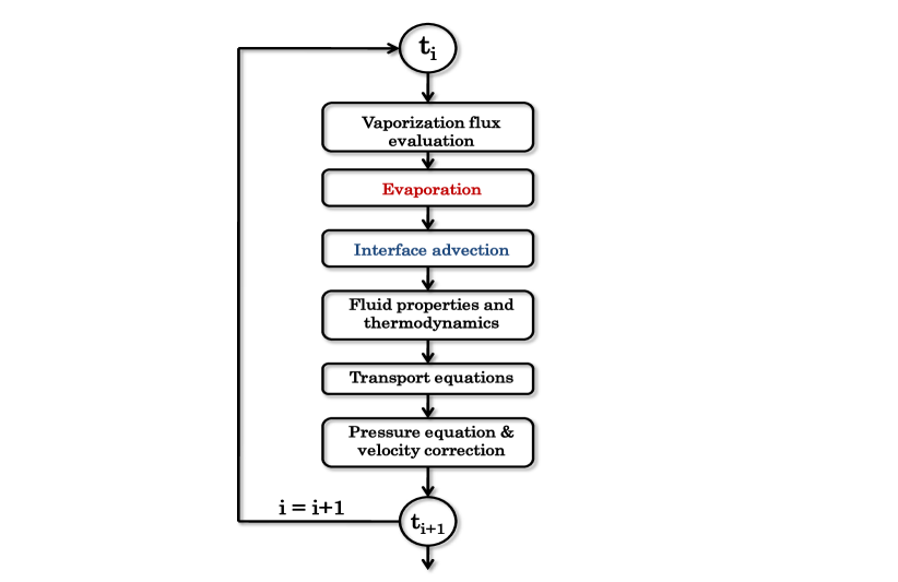
Figure 3: Steps of the numerical algorithm used in DropletSMOKE++

3.1 Description of the DropletSMOKE++ solver

The DropletSMOKE++ code is embedded within the $\texttt{OpenFOAM}^{\textregistered}$ framework which allows to manage the spatial discretization of the governing equations on arbitrary geometries. The PIMPLE algorithm [greenshields2015openfoam], a combination between SIMPLE (Semi-Implicit Method for Pressure-Linked Equations) and PISO (Pressure Implicit Splitting of Operators), is used to manage the pressure-velocity coupling, computing a velocity field which satisfies both momentum and continuity equation through an iterative procedure.
For every time step, DropletSMOKE++ encompasses the following steps in a segregated approach (Figure 3):

1. Evaluation of the evaporation flux (Equation 16)

2. Liquid evaporation or expansion (Equation 4)

3. Interface advection (Equation 3)

4. Update of gas-liquid properties and thermodynamics

5. Momentum, temperature and species equation (Equations 30, 8, 9)

6. Iterative calculation of the pressure field (Equation 7) and velocity correction

The time discretization follows an implicit Euler method, where the time step is automatically computed based on a threshold Courant number. As reported by Brackbill et al. [brackbill1992continuum], the VOF time step constraint states that $\Delta t<\left[\frac{\rho\left(\Delta x\right)^{3}}{2\pi\sigma}\right]^{\frac{1}{2}}$, which depends on surface tension. It is worth noticing that the suppression of surface tension introduced in this work alleviates this constraint, allowing larger time steps to be used.
Finally, Gauss linear upwind scheme is used for spatial discretization of convective terms, while an orthogonal correction is adopted for Laplacian terms.

Boundary	$\alpha$	v	T, $\omega_{i}$	$p_{rgh}$
inlet (natural convection)	$\alpha=0$	inletOutlet	inletOutlet	$p_{rgh}=p_{ext}$
inlet (forced convection)	$\alpha=0$	$\textbf{v}=\textbf{v}_{ext}$	$T,\omega_{i}=T_{ext},\omega_{i,ext}$	$\nabla p_{rgh}=0$
outerWall	$\alpha=0$	noSlip	$\nabla T,\nabla\omega=0$	$\nabla p_{rgh}=0$
outlet	$\alpha=0$	inletOutlet	inletOutlet	$p_{rgh}=p_{ext}$
sphere	$\nabla\alpha=0$	noSlip	$\nabla T,\omega=0$	$\nabla p_{rgh}=0$

Table 1: Boundary conditions for $\alpha$, velocity, temperature, species $i$ and pressure field, to be compared with Figure 4.

3.1.1 Computational mesh

The computational mesh used for all the numerical cases proposed in this work has been built with the commercial CFD code $\texttt{Ansys FLUENT}^{\textregistered}$ v17.2. The geometry is 2D and axisymmetric, representing a slice of a cylinder having a radius $W=5$ mm and a height $H=30$ mm. At 10 mm from the base a spherical fiber (diameter $D=0.1$ mm) is introduced, which is needed as a source for the force field $\textbf{f}_{m}$ previously described. The liquid droplet will be place around this small spherical fiber.

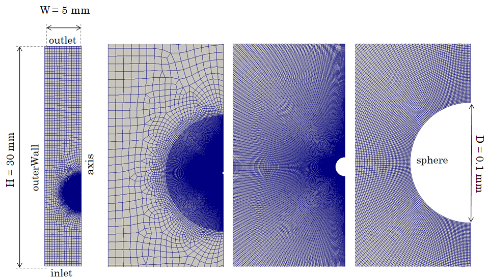
Figure 4: Computational mesh represented in increasing levels of detail, from left to right. The boundary names are also shown, to be compared with Table 1.

The geometry is meshed in a non-structured way (Figure 4), with a particular attention to the gas-liquid boundary: the mesh is structured and orthogonal on the cylinder boundaries. The region including the liquid droplet and the gas in its proximity is meshed with a concentric pattern, getting finer while approaching the inner fiber. Therefore, the presence of a spherical boundary is also necessary for the mesh construction.
In this work, the mesh is composed by 70,000 cells, with a maximum mesh non-orthogonality equal to 56.6 and a maximum Skewness of 1.3. It has been verified that the numerical solution does not change doubling the number of cells, proving a complete mesh independence.

(a)

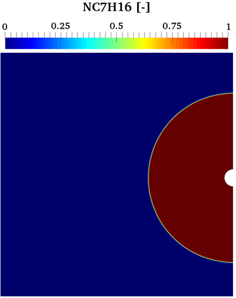
(b)

(c)

Figure 5: Example of initial conditions in droplet evaporation simulations. Liquid volume fraction ($\alpha$ field) in Figure (a), n-heptane mass fraction in Figure (b) and temperature field in Figure (c).

3.2 Boundary conditions

The definition of proper boundary conditions is fundamental to reach reliable results. The geometry has four boundaries, shown in Figure 4:

1. outerWall: external lateral surface of the cylinder

2. inlet: the bottom base surface of the cylinder

3. outlet: the upper base of the cylinder

4. sphere: the spherical fiber surface

The boundary conditions are summarized in Table 1. The $inlet$ boundary conditions change depending on the case (natural or forced convection). The $inletOutlet$ condition is basically a zero gradient condition, that switches to a fixed value condition if the velocity vector next to the boundary points inside the domain (backward flow). The $noSlip$ condition imposes a zero relative velocity between the fluid and the boundary. It is worth noticing that the separation of the hydrostatic pressure, allows a simple definition of boundary conditions for $p_{rgh}$.

3.3 Initial conditions

Referring to the mesh presented in Figure 4, the liquid droplet must be positioned around the spherical fiber. In Figure 5 the initial conditions for the evaporation of a cold n-heptane droplet in a hot environment are presented as an example.

3.4 Code parallelization

Case	Species	$D_{0}$	$T_{L}$	$T_{G}$	p	Results
		[mm]	[K]	[K]	[atm]	[Figure 6]
1	n-Decane	0.5	435	435	1	(a, b, c)
2	n-Heptane	0.5	360	360	1	(d, e, f)
3	n-Heptane	1.03	300	364	20	(g, h, i)
4	Water	0.7	360	360	1	(j, k, l)

Table 2: Numerical cases for the comparison with 1D model [cuoci2005autoignition]. The related plots are reported in Figure 6.

The numerical cases presented in this work are run on a multi-processor (Intel Xeon X5675, 3.07 GHz) machine. The Domain Decomposition Method is used to split the mesh into sub-domains and allocate them to separate processors. The DropletSMOKE++ code can then run in parallel mode, with communication between processors with MPI communication protocol, allowing a significant reduction of the computational time. The optimal number of processors is found to be around 12, which corresponds to an average of 6000 cells for each processor and a speed-up performance $\sim$ 6 times higher with respect to the serial mode.
The simulations required from 2 to 20 hours, depending on the operating conditions.

4 Validation of microgravity cases

In this section DropletSMOKE++ is validated in microgravity conditions (imposing $\textbf{g}=\textbf{0}$), against the numerical results of the solver developed by Cuoci et al. [cuoci2005autoignition]. This latter code has been validated in a wide range of operating conditions over the last 10 years [stagni2018numerical, cuoci2017flame] and represents a reliable reference for comparison. This validation is done in order to assess the validity of the equations (in terms of diameter decay, temperature profiles and vaporization velocity) before the activation of the gravity field. Obviously, the centripetal force $\textbf{f}_{m}=0$ in these cases.

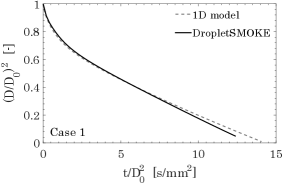
(a)

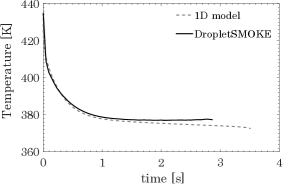
(b)

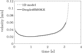
(c)

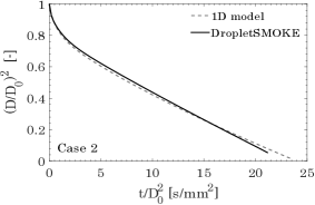
(d)

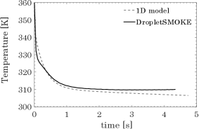
(e)

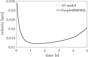
(f)

(g)

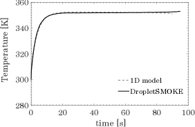
(h)

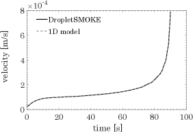
(i)

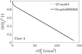
(j)

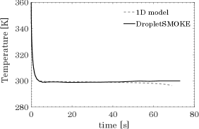
(k)

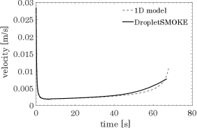
(l)

Figure 6: Numerical comparison of the 1D model of Cuoci et al. [cuoci2005autoignition] and DropletSMOKE++ (Table 2).

The 4 numerical cases analyzed are listed in Table 2. Three liquids have been chosen (n-decane, n-heptane and water) at different temperature and pressure conditions. Numerical results are summarized in Figure 6.
For each case (lines) three plots are reported (columns): the temporal evolution of the droplet size, the liquid surface temperature and the vaporization velocity. More precisely, this latter is the convective velocity of the gas generated at the phase boundary.

4.1 Results and discussion

For all cases the squared diameter, after the initial transient period, reduces linearly with time, as the $d^{2}$ law states. A wet-bulb temperature is reached by the interface and maintained along the whole evaporation process, due to the equilibrium between the incoming heat flux and the outcoming vaporization enthalpy. The transient period depends on the initial conditions. In cases 1-2-4 (initially isothermal) the interface is immediately cooled, diminishing the vaporization flux. In case 3 the liquid is firstly heated (reducing $\rho_{L}$ and increasing the droplet size) providing an increasing vaporization flux.
The agreement between the models can be considered satisfactory, even if small differences exist. In particular the surface temperature tends to be slightly over-predicted, especially in the final steps of the evaporation. This is probably due to the spherical boundary of the fiber in the DropletSMOKE++ simulations (Figure 4), which is absent in the 1D model. The presence of a small sphere inside the liquid provides a lower droplet mass if compared to a 1D droplet with the same initial diameter. As can be seen in Figure 6 its effect is completely negligible for most of the simulation (the ”missing” mass is less than $0.01\%$ of the initial total mass). While the droplet surface approaches the fiber, this effect becomes important: the incoming heating flux is now distributed over a lower liquid mass, providing a slightly higher equilibrium temperature. This will not be a problem when modeling evaporation under convection, since fibers are always present in experiments to hang liquid droplets.

5 Implementation of the centripetal force $\textbf{f}_{m}$

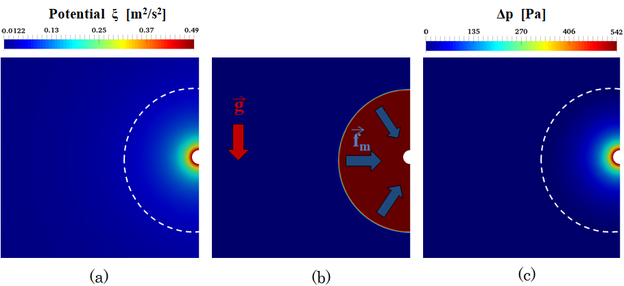
Figure 7: Potential field $\xi$ (Figure a) around fiber, evaluated with $\xi_{0}=1$ $m^{2}/s^{2}$. In Figure (b) the droplet is placed around the fiber and sustained against gravity g by the force $\textbf{f}_{m}=\rho\alpha\nabla\xi$. The $\Delta p=p-p_{ext}$ field is presented in Figure (c). The white dashed lines in (a,c) represent the droplet surface.

In order to sustain the droplet against the gravity field, a centripetal force $\textbf{f}_{m}$ (Equation 28) is introduced, based on a potential $\xi$ defined by Equation 29, represented in Figure 7 (a) and previously described in the mathematical model. The liquid droplet is then fixed around the fiber (Figure 7 b). Inside the droplet a small pressure gradient is established (from $\sim$100 to $\sim$500 Pa, depending on the value $\xi_{0}$), similarly to what happens for a liquid column subjected to a gravity field (Figure 7 c). This is actually consistent with surface tension forces, which provide an internal pressure higher than the external one (capillary pressure).

5.1 Control of the droplet shape

A droplet suspended under the effect of a gravity field reaches a steady-state shape imposed by the equilibrium between the liquid weight, the pressure gradient and the surface tension forces:

$$-\nabla p+\sigma\kappa\nabla\alpha+\rho\textbf{g}=\textbf{0}$$ (32)

In this work surface tension in not considered, and the centripetal force $\textbf{f}_{m}$ governs the equilibrium shape of the droplet:

$$-\nabla p+\textbf{f}_{m}+\rho\textbf{g}=\textbf{0}$$ (33)

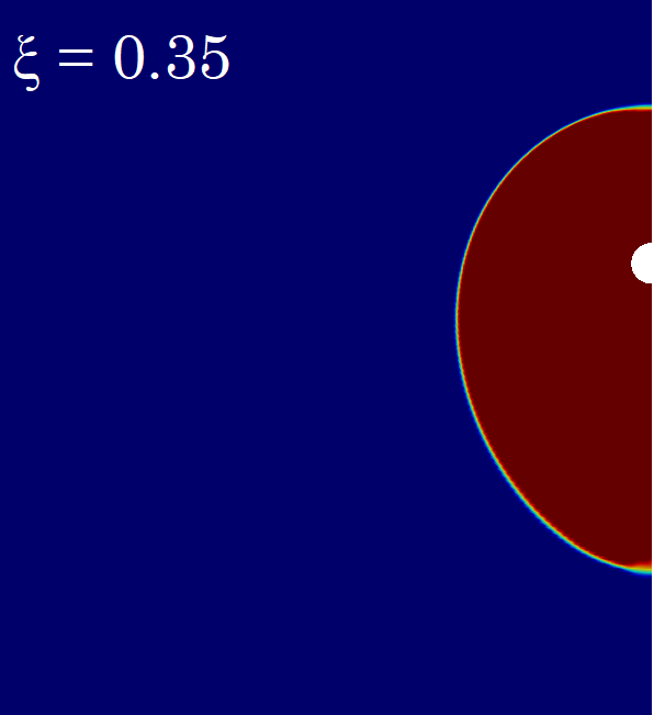
(a)

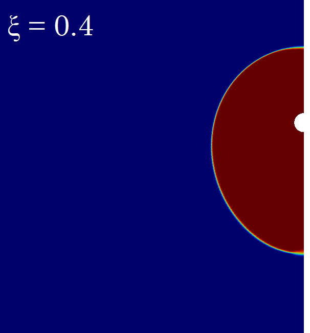
(b)

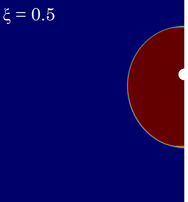
(c)

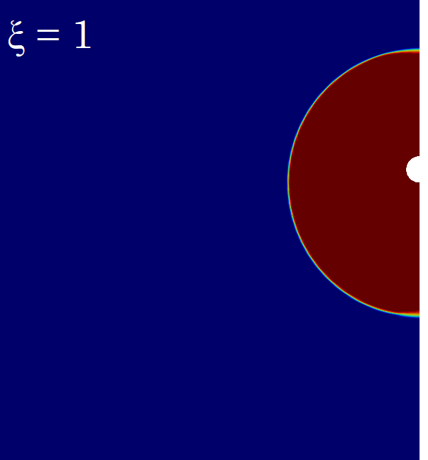
(d)

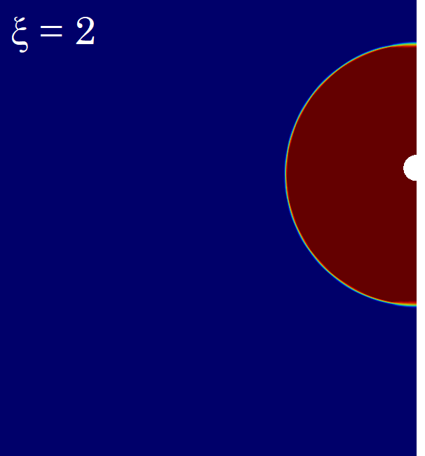
(e)

Figure 8: Equilibrium shape of a n-heptane droplet ($D_{0}=1$ mm, ambient $T$) under the effect of gravity g and different intensities of the potential field $\xi_{0}\left[\frac{m^{2}}{s^{2}}\right]$.

The intensity of $\textbf{f}_{m}$ can be controlled by the value of the constant $\xi_{0}$, which defines the potential field $\xi$ (Equation 29). Figure 8 shows the equilibrium shape assumed by a n-heptane droplet (1 mm diameter, ambient $T$) for different values of $\xi_{0}$, from 0.35 to 2 $\frac{m^{2}}{s^{2}}$. For values $\xi_{0}<0.35$ $\frac{m^{2}}{s^{2}}$ the droplet falls down, while for $\xi_{0}>2$ $\frac{m^{2}}{s^{2}}$ the droplet shape remains spherical. These threshold values have been found to be nearly the same for different liquids.
The effect is very similar to surface tension forces: for low values of $\xi_{0}$ (or surface tension $\sigma$) the droplet tends to assume an elongated shape, because of the dominant gravity forces. Increasing $\xi_{0}$ (or surface tension $\sigma$), the droplet approaches a spherical geometry. In this work $\xi_{0}$ represents a degree of freedom of the problem, which we can saturate imposing a $\xi_{0}$ value that better describes the droplet shape of the experimental cases.

5.2 Effect of the droplet shape on evaporation

In order to set a proper initial shape of the droplet, a sensitivity analysis on the evaporation process has been carried out. Two numerical simulations of an evaporating n-heptane droplet have been run for the threshold values $\xi_{0}=0.35$ $\frac{m^{2}}{s^{2}}$ and $\xi_{0}=2$ $\frac{m^{2}}{s^{2}}$, (Figures 8 a, e). The initial droplet diameter $D_{0}=1$ mm, the liquid temperature is $T_{L}=300$ K, the ambient temperature is $T_{G}=364$ K and the pressure is $p=20$ bar.
From Figure 9 we can see that the droplet shape does not have a major impact on the evaporation process. The surface area increases for lower values of $\xi_{0}$, explaining the slightly larger evaporation rates (Figure 9 c), while the surface temperature (Figure 9 b) is almost insensitive to $\xi_{0}$.
We expect the experimental cases of our interest to behave somewhere in-between these two cases, closer to the upper limit described by the black lines in Figure 9
In order to verify this hypothesis, a simple analysis has been conducted on the droplet shapes usually involved in experiments. 10 pictures of suspended droplets available in literature from experimental works [ghassemi2006experimental, matlosz1972investigation, morin2004vaporization, han2015evaporation, walton2004evaporation, chauveau2008experimental, suzuki2009development] have been collected (Figure 10 b) and organized based on two dimensionless numbers, the sphericity $\psi$ and the Eötvös number $Eo$, defined as:

$$\psi=\frac{D_{y}}{D_{x}}$$ (34)

$$Eo=\frac{\left(\rho_{L}-\rho_{G}\right)gD^{2}}{\sigma}\sim\frac{\rho_{L}gD^{2}}{\sigma}$$ (35)

where $D_{y}$ and $D_{x}$ are the maximum lengths of the droplet, in vertical and horizontal directions. The sphericity $\psi$ is a measure of how the droplet shape approaches that of a perfect sphere (which has $\psi=1$). The Eötvös number $Eo$ is the ratio between gravitational and surface tension forces. A further classification is introduced based on the tipe of supporting fiber (vertical, horizontal or cross fiber). The 10 experimental cases are reported in Figure 10 (a), together with the black line $\psi=1$, representing a perfect sphere (Figure 8 e), and the gray line $\psi=1.2$ representing the limit case in Figure 8 (a).

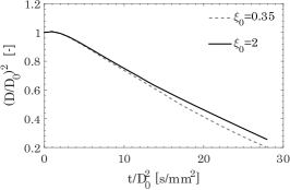
(a)

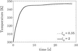
(b)

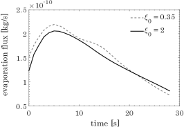
(c)

Figure 9: Effect of the droplet shape on the evaporation process. The dashed grey line corresponds to Figure 8 (a), while the black line refers to Figure 8 (e).

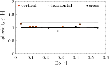
(a)

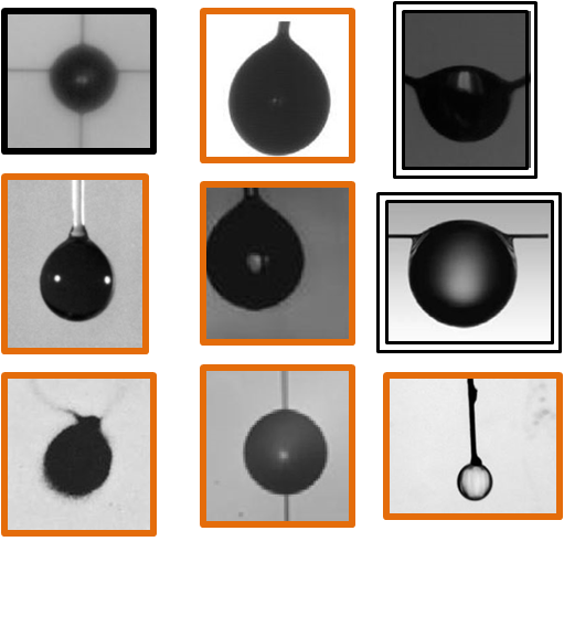
(b)

Figure 10: Scatterplot of experimental cases of suspended droplets (Figure a), based on their Eötvös number $Eo=\frac{\rho_{L}gD^{2}}{\sigma}$ and sphericity $\psi=\frac{D_{y}}{D_{x}}$. Colors represent the supporting fiber: vertical (orange), horizontal (white) and cross fiber (black). The black line represents a perfect sphere ($\psi=1$), the gray line represents the limit case in Figure 8 a ($\psi=1.2$). Figure (b) reports the 9 of the 10 droplet pictures, signed with the same colors for comparison.

The Eötvös number is below 1 for all cases, indicating that surface tension forces always dominate over gravity. The sphericity $0.86<\psi<1.12$ indicates nearly spherical shapes for all the droplets, especially when cross fibers are used (black points). As expected, the horizontal fibers tend to slightly deform the droplet along $D_{x}$ direction, providing $\psi<1$ (white points) while the vertical ones along $D_{y}$, providing $\psi>1$ (orange points). Figure 10 clearly shows that most of experimental cases lay between the two lines $\psi=1$ (Figure 8 e) and $\psi=1.2$ (Figure 8 a). A rigorous modeling of the surface topology would require different computational meshes to describe the large variety of fibers used to support the droplets (vertical, horizontal, thermocouples, cross fibers…), as well as precise data regarding the dynamic contact angle between the solid and the different liquids. In order to simplify the problem and based on Figures 9 and 10, we assume the evaporation regime not to be significantly influenced by small deviations of the droplet shape from the spherical one, which probably better describes on average the different experimental cases analyzed in this work. For these reasons we decided to adopt an intermediate value $\xi_{0}=1$ $\frac{m^{2}}{s^{2}}$ (Figure 8 d).

6 Cases in natural convection

6.1 Description of the experimental cases

The numerical model is now validated against 11 sets of experimental data in natural convection regime, taken from 4 papers in literature from 1997 to 2018. All the experimental cases are summarized in Table 3.
Ghassemi [ghassemi2006experimental] used a fine quartz fiber of 0.125 mm of diameter (similarly to the spherical fiber used in our simulations) to hang and evaporate small n-heptane droplets in a hot nitrogen environment. Nomura et al. [Nomura1997] examined the evaporation of cold n-heptane droplets in a hot air environment from 300 K to 450 K at various pressures (from 5 atm to 50 atm). The experimental data are taken from the paper of Gogos et al. [gogos2003effects], who proposed a very complex axysimmetric model to model them. An aluminum cross-fiber support frame has been utilized by Verwey et al. [verwey2018experimental], in order to maintain a spherical shape of the droplet. N-decane and n-heptane evaporation has been investigated. Finally, n-hexadecane droplets evaporation was examined through a horizontal fiber by Han et al. [han2015evaporation]. Where needed, electric furnaces have been used to heat up the environment and nitrogen to pressurize the vessel. High-speed video cameras have been adopted to follow the droplet lifetime. For all cases, the experimental data provided concern the droplet ”equivalent” diameter decay. Han et al. [han2015evaporation] also provided some data on the mean droplet temperature by using a thermocouple as a fiber.
To our knowledge, the cases from Verwey et al. [verwey2018experimental] and Han et al. [han2015evaporation] have never been modeled. Experimental data from Ghassemi et al. [ghassemi2006experimental] and Nomura et al. [Nomura1997] have only been approached so far either with simplified semi-analytical methods, or specific correlations based on mass-heat transfer dimensionless numbers for the evaporation sub-model [azimi2017effect, fang2017new].
In principle, the DropletSMOKE++ code can handle the thermal perturbation of the fiber on the droplet. This could be done either imposing a heat flux of the sphere boundary (Figure 5) which mimics its presence, or directly meshing the fiber geometry and solve the multi-region heat transfer between the fluid and the solid. Because of the small size of the fibers used in the experiments and the relatively low temperatures involved (since we are not modeling combustion processes), we found the evaporation process to be marginally affected by the thermal perturbation of the fiber, deciding to neglect it and postponing the problem to future works.

Case	Species	$D_{0}$	$T_{L}$	$T_{G}$	p	Refs.	Results
		[mm]	[K]	[K]	[atm]
1	n-Heptane	1	300	773	10	[ghassemi2006experimental]	Figure 12 (a)
2	n-Heptane	1	300	673	10	[ghassemi2006experimental]	Figure 12 (b)
3	n-Heptane	0.698	300	398	50	[Nomura1997]	Figure 13 (a)
4	n-Heptane	0.607	300	474	10	[Nomura1997]	Figure 13 (b)
5	n-Heptane	0.604	300	450	5	[Nomura1997]	Figure 13 (c)
6	n-Decane	0.546	300	373	10	[verwey2018experimental]	Figure 14 (a)
7	n-Heptane	0.539	300	300	5	[verwey2018experimental]	Figure 14 (b)
8	n-Decane	0.5	300	300	1	[verwey2018experimental]	Figure 14 (c)
9	n-Decane	0.245	300	300	10	[verwey2018experimental]	Figure 14 (d)
10	n-Hexadecane	1	300	773	1	[han2015evaporation]	Figure 15 (a, b, c)
11	n-Hexadecane	1	300	673	1	[han2015evaporation]	Figure 15 (d, e, f)

Table 3: Experimental cases in natural convection regime examined in this work.

6.2 Numerical simulations: results and discussion

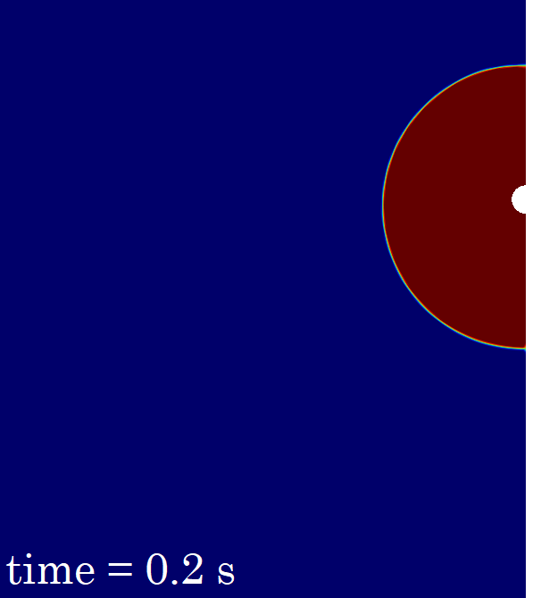
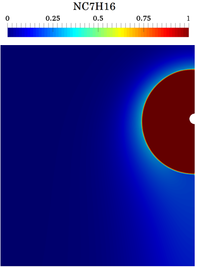
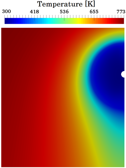
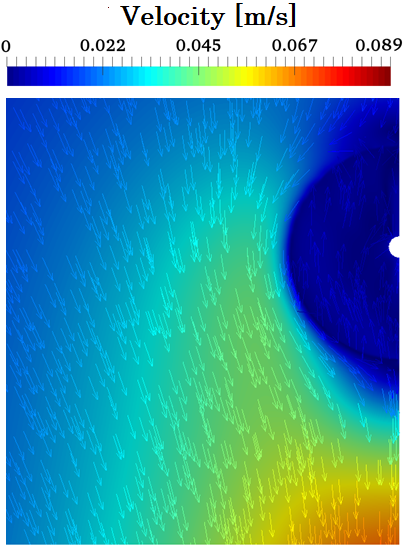
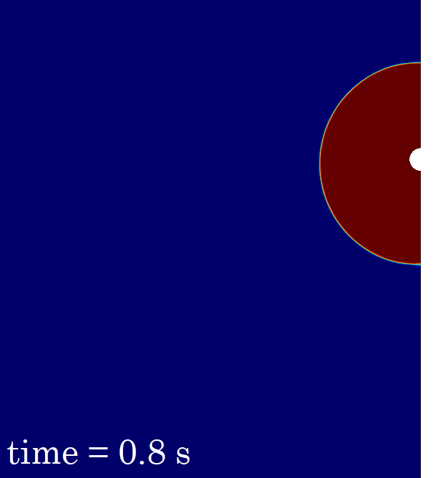
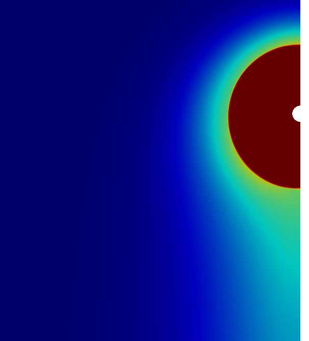
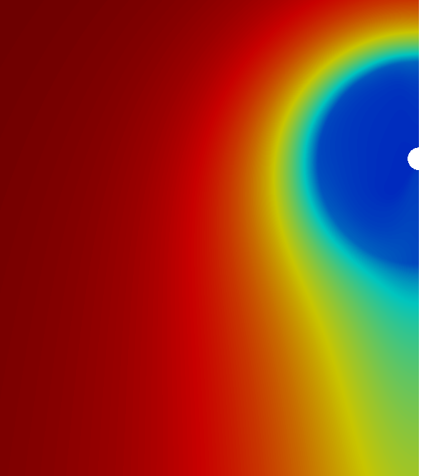
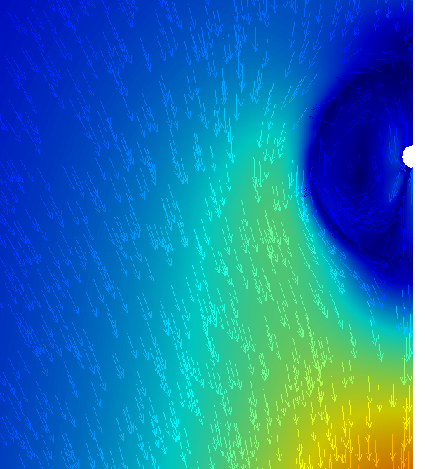
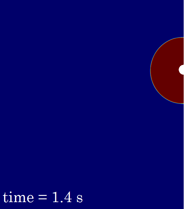
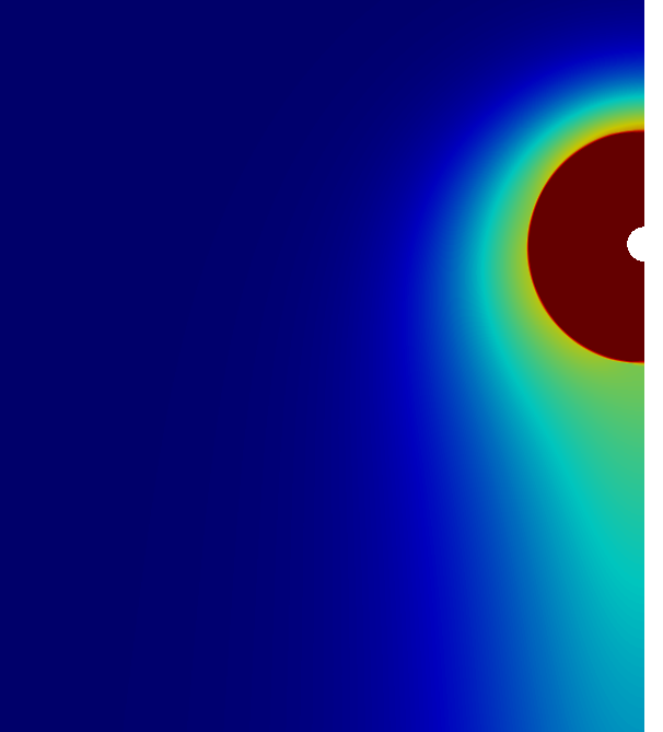
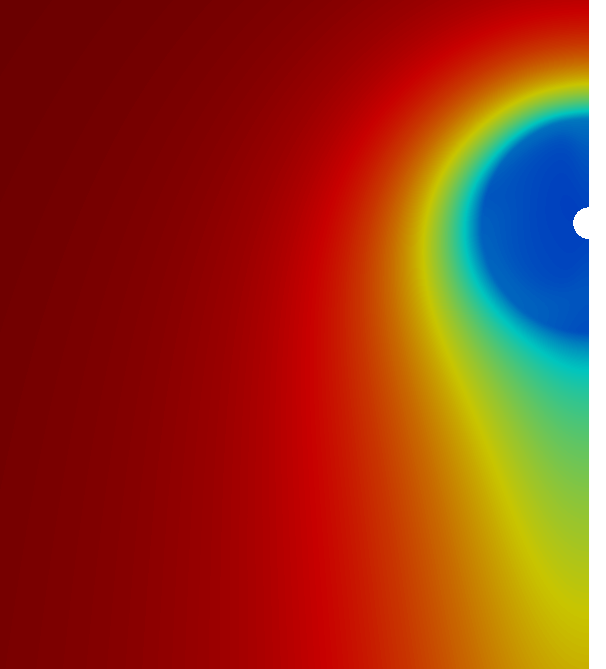
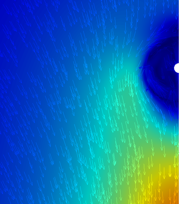
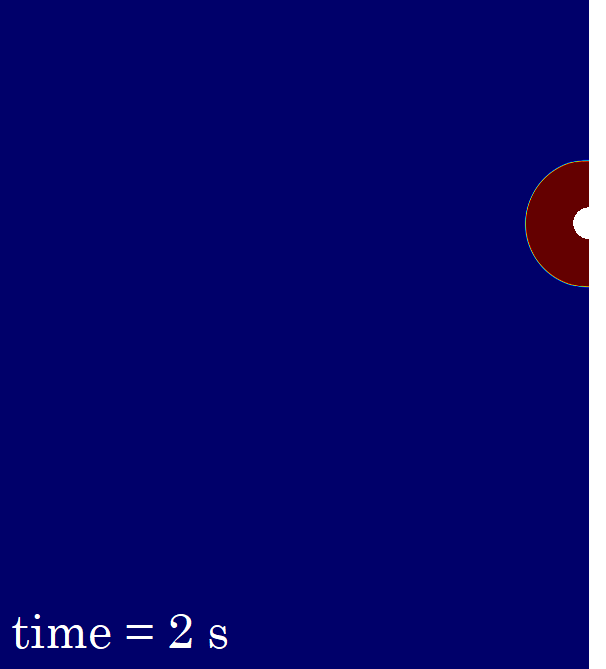
(a)

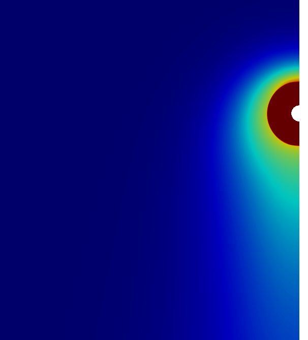
(b)

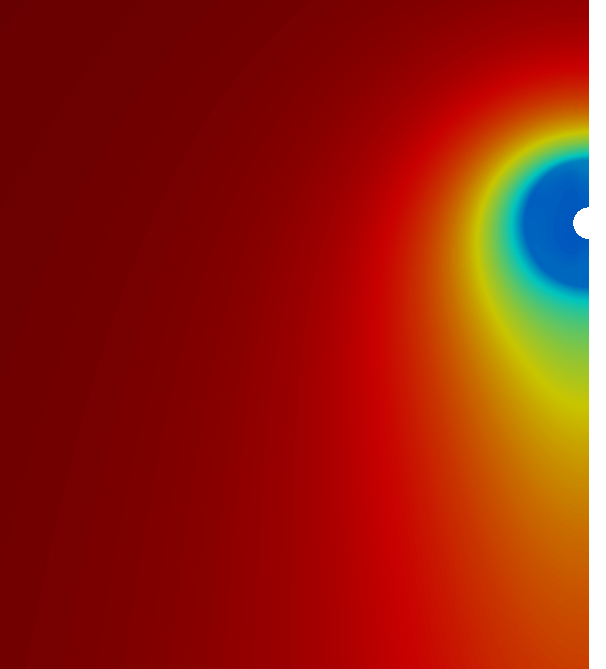
(c)

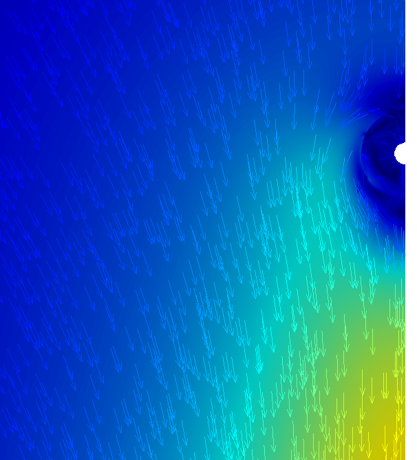
(d)

Figure 11: $\alpha$ (a), n-heptane mass fraction (b), temperature (c) and velocity vector fields (d) evolution. Numerical simulation of case 1 from Ghassemi et al. [ghassemi2006experimental].

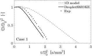
(a)

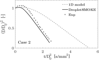
(b)

Figure 12: Model prediction of the experimental data of Ghassemi et al. [ghassemi2006experimental], cases 1, 2 of Table 3.

For each one of the cases presented in Table 3, an equivalent simulation (imposing the same initial conditions) has been performed with the microgravity solver of Cuoci et al. [cuoci2005autoignition] in order to highlight the impact of gravity on the numerical simulation and better support the need of a multidimensional CFD model.
In Figure 11 the numerical results of the simulation of case 1 of Ghassemi et al. [ghassemi2006experimental] are reported as a reference example for a qualitative analysis. The liquid volume fraction ($\alpha$), the n-heptane mass fraction field, the temperature and the vectorial velocity field are reported respectively in Figures 11.
The droplet is initially at an ambient temperature $T_{L}=300$ K and it is progressively heated by the external environment at $T_{G}=773$ K (Figure 11 c). A small amount of vapor is released from the droplet surface (Figure 11 b). The gas around the droplet is cooler than $T_{G}$ and the n-heptane vapor has a higher density. This density gradient induces a downward flow field (Figure 11 d) around the droplet, generating a laminar natural convection regime. After a transient period, an equilibrium temperature is reached since the equilibrium mass fraction vapor in Figure 11 (b) reaches a steady state value.

Figure 12 reports the numerical results of the cases from Ghassemi et al. [ghassemi2006experimental] (cases 1, 2), compared against the available experimental data. DropletSMOKE++ can predict the experimental data with a reasonable accuracy for both cases. The linear behavior of the squared diameter can be easily recognized, as well as its initial increase due to the droplet heating shown in Figure 11.

The numerical simulations of the cases from Nomura et al. [Nomura1997] (cases 4, 5, 6) are reported in Figure 13. There is a good agreement with the experimental data, especially if compared to the model prediction of the 1D model which largely overpredicts evaporation times. The velocity field around the droplet increases both heat and mass transfer rates from the liquid surface, providing a much lower evaporation time with respect to the microgravity case. This effect is particularly enhanced at high pressure (case 3, Figure 13 a) where the droplet evaporates $\sim 4$ times faster under the influence of gravity.
The reason is straightforward: the Grashof number increases with the gas density (with a power 2), which is proportional to pressure:

$$Gr=\frac{\rho^{2}gD^{3}\beta\Delta T}{\mu^{2}}\sim p^{2}$$ (36)

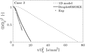
(a)

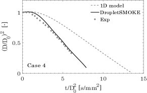
(b)

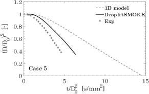
(c)

Figure 13: Model prediction of the experimental data of Nomura et al. [Nomura1997], cases 3, 4, 5 of Table 3.

Therefore, the presence of natural convection has a stronger impact in high pressures cases, if compared with the same cases in microgravity (where $Gr=0$).
In Case 5 (Figure 13 c) we slightly overpredict the droplet lifetime, especially if compared to the other cases from the same author. It is worth noticing that this experimental case has been also modeled by Gogos et al. [gogos2003effects], using a complex non-VOF axisymmetric model and assuming a perfectly spherical droplet. His model generally shows good agreement with experiments, but the results of this specific case show deviation from the experimental data very similar to ours.

The cases from Verwey et al. [verwey2018experimental] are carried out in mild conditions, characterized by a low vaporization rate due to the low temperatures and moderately high pressures involved. This is clear from Figure 14, where the evaporation times are much longer with respect to the previous cases. Cases 8 and 9 are particularly interesting, since the microgravity solver predicts a quasi steady-state condition. An evaporation flux is still present, but it is extremely low due to the purely diffusive regime involved (the Stefan flow in this conditions is completely negligible). It is interesting to point out that the velocity flow around the droplet has a maximum magnitude value of only 0.5-0.6 mm/s (not shown). Despite this small convective flow, the evaporation rate is strongly enhanced.

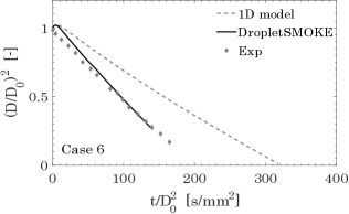
(a)

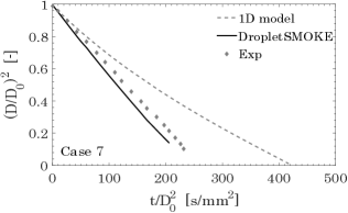
(b)

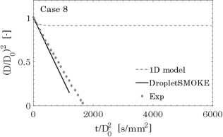
(c)

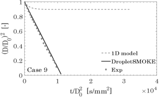
(d)

Figure 14: Model prediction of the experimental data of Verwey et al. [verwey2018experimental], cases 6, 7, 8, 9 of Table 3.

This can be easily analyzed by scaling arguments: in case 8 (Figure 14 c) the initial droplet diameter is $D_{0}=0.5$ mm, while the surrounding convective flow has an average magnitude of $0.5$ mm/s. This means that, taking the droplet diameter $D_{0}$ as a characteristic length of the system, the complete replacement of vapor cloud around the droplet lasts $\sim 1$ s, while for the pure diffusion case is practically infinite.

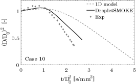
(a)

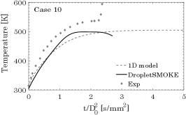
(b)

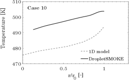
(c)

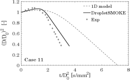
(d)

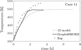
(e)

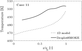
(f)

Figure 15: Figures (a), (b), (d), (e) show the model prediction of the experimental data of Han et al. [han2015evaporation], cases 10, 11 of Table 3. Figures (c), (f) report the liquid temperature distribution predited by DropletSMOKE++ and by the 1D model for cases 10, 11 (time = 2 s).

n-Hexadecane droplets evaporation from Han et al. [han2015evaporation] have been modeled (Figure 15). Experimental data on the mean droplet temperature are also available. There is a good agreement with the experimental results. The droplet temperature is slightly underestimated, especially towards the end of the simulation. Experimentally, this is due to the exposure of the thermocouple to the hot gas when the droplet is almost entirely consumed, or to the additional heat flux on the droplet given by the heat conduction from the fiber.
Figures 15 (c), (f) show the liquid temperature distribution inside the droplet predicted with the 1D model and with DropletSMOKE++, for both Cases 10-11, at time $t=2$ s. The heat flux on the droplet surface is rapidly redistributed inside the liquid phase because of the internal circulation, as will be further discussed later. This provides an average liquid temperature which is higher if compared to the 1D model. Moreover, the temperature distribution predicted by DropletSMOKE++ is more homogeneous, while stronger $T$ gradients characterize the 1D model.

Whereas the evaporation rate and the droplet lifetime are strongly influenced by natural convection, in terms of droplet surface temperature there is no significant deviation between the 1D model and DropletSMOKE++. More precisely, the initial droplet heating is faster (since evaporation is here negligible), but the steady state wet-bulb temperature is the same. The experimental data confirm this fact (Figure 15 b, e).
In steady state conditions, there is an equilibrium between the heat flux on the droplet surface and the evaporating flux enthalpy:

$$h_{T}\left(T_{G}-T_{s}\right)=h_{M}\left(\rho_{i,s}-\rho_{i,G}\right)\Delta h_{ev,i}$$ (37)

where $\rho_{i,s}=\frac{p_{i}^{0}\left(T_{s}\right)M_{w,i}}{RT_{s}}$ is the surface vapor concentration, while $\rho_{i,G}\sim 0$. $h_{T}$ is the external heat transfer coefficient, while $h_{M}$ is the external mass transfer coefficient. It is possible to derive one coefficient from the other through the Chilton-Colburn factor $J$ [bird2002transport]:

$$J_{M}=\frac{Sh}{ReSc^{\frac{1}{3}}}=J_{T}=\frac{Nu}{RePr^{\frac{1}{3}}}$$ (38)

from which it is easy to derive $h_{M}$ in function of $h_{T}$:

$$h_{M}=\frac{\mathcal{D}_{i}}{k}\left(\frac{Sc}{Pr}\right)^{\frac{1}{3}}h_{T}$$ (39)

substituting $h_{M}$ in Equation 37:

$$T_{G}-T_{s}=\frac{\mathcal{D}_{i}}{k}\left(\frac{Sc}{Pr}\right)^{\frac{1}{3}}\frac{p_{i}^{0}\left(T_{s}\right)M_{w,i}}{RT_{s}}\Delta h_{ev,i}$$ (40)

The resolution of this equation provides the equilibrium temperature $T$. Equation 40 clearly indicates that the wet-bulb temperature does not depend on the external fluid flow, but only on the properties of the fluids and on the bulk temperature $T_{G}$.

Case	Species	$D_{0}$	$T_{L}$	$T_{G}$	p	$|\textbf{v}|$	Refs.	Results
		[mm]	[K]	[K]	[atm]	[m/s]
1	n-Heptane	0.7	300	490	1	0.7	[yang2002experimental]	Figure 16 (a)
2	n-Hexadecane	0.7	300	490	1	0.7	[yang2002experimental]	Figure 16 (b)

Table 4: Experimental cases in forced convection regime examined in this work.

7 Cases in forced convection

7.1 Description of the experimental cases

To conclude this work, two cases in forced convection have been simulated and compared with experimental results taken from Yang et al. [yang2002experimental]. According to our knowledge, this is the first time that these cases are numerically modeled. n-heptane and n-hexadecane droplets have been evaporated in an upward hot gas flow generated by a heating coil. The experimental data are given for different supporting fibers diameters. The data chosen for comparison refer to a fiber diameter of 0.15 mm, which is the closest to the fiber dimension used in this work ($D$ = 0.1 mm). The experimental cases are summarized in Table 4.

7.2 Numerical results and discussion

The boundary conditions presented in Table 1 impose a fixed upward velocity at the $inlet$ boundary, as well as a fixed temperature value. In Figure 16 (c) we can see the upward velocity field and the relative effect on the vapor cloud around the droplet and on the temperature field.
The agreement with the experimental data (Figure 16 a, b) is satisfactory, with a slight overestimation of the initial heat up in case 2.

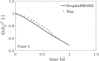
(a)

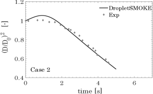
(b)

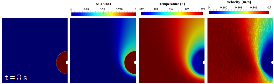
(c)

Figure 16: Figure (a): model prediction of the experimental data of Yang et al. [yang2002experimental], cases 1 (a) and 2 (b) of Table 4. Figure (c): $\alpha$, n-hexadecane mass fraction, temperature and velocity fields at time $t=3$ s, of the numerical simulation of case 2.

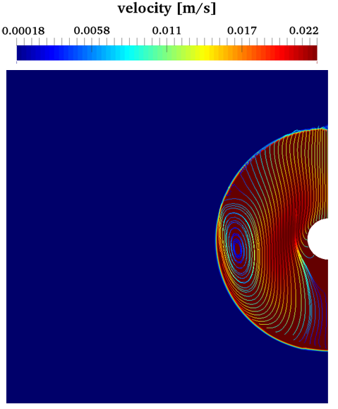
(a)

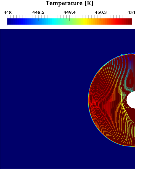
(b)

Figure 17: Flow field streamlines in the liquid phase for case 2 (Table 4), time $t=3$ s. Colored by velocity magnitude (a) and temperature (b).

From Figure 16 (c), it is clear that the liquid phase can be considered almost uniform in these conditions. This is further analyzed in Figure 17: the flow field streamlines are reported for the liquid phase, colored by the velocity magnitude (Figure 17 a) and temperature (Figure 17 b) for case 2 (Table 4) at time $t=3$ s. The external convective flow induces a shear stress on the surface providing a strong circulation inside the droplet, with a maximum magnitude of $\sim$ 2 cm/s. The resulting toroidal structure is well known in literature, and it is usually approximated as an inviscid Hill’s spherical vortex [sirignano1999fluid, lamb1945hydrodynamics] to derive sub-models of droplet heating. It has been demonstrated that internal circulation needs to be included in modeling droplet vaporization [kotake1969evaporation], and this is usually accomplished with effective conductivity models [abramzon1989droplet]. Since the entire flow field is directly solved in this work, the internal temperature field can be predicted with no need of such additional sub-models. The maximum temperature difference inside the liquid phase is only $\sim$ 3 $K$ (Figure 17 b). As expected, a more intense heat transfer occurs at the bottom of the droplet, where the flow field impacts the liquid.
Finally, it is important to point out that the suppression of surface tension forces adopted in this work could in principle affect the internal motion in the liquid phase, because of the different the tangential shear stress at the interface. However, our comparative analyses in this sense, not reported in this work, show that the results obtained with DropletSMOKE++ are in a reasonable agreement both with experimental [mandal2012internal, mandal2012evidence] and numerical [george2017detailed, sim2015computational] works not based on the VOF methodology. These investigations are still preliminary, but indicate that even neglecting surface tension the internal circulation phenomenon can be quantitatively and qualitatively captured with a reasonable accuracy.

8 Conclusions

In this work we presented a multidimensional CFD numerical framework for the evaporation of isolated fuel droplets. The solver (called DropletSMOKE++) accounts for the presence of external flow field and for the influence of a gravity field, allowing to numerically model the evaporation of droplets both in natural and forced convection. The code is embedded within the well-known $\texttt{OpenFOAM}^{\textregistered}$ framework, open for contributions from the scientific community.
The core of the code is based on the VOF (Volume Of Fluid) methodology, widely known for its simplicity and mass conservation properties. The interface is geometrically advected and subjected to source terms to account both for evaporation and liquid expansion. This main solver is coupled with an evaporation model, which directly computes the vaporization rate from the interface molar fraction gradient, and with energy and species equations.
The main novelty of this work is the surface tension treatment. The parasitic currents, still an open problem for the modeling of small droplets dynamics, have been completely suppressed by-passing the modeling of surface tension effects. A centripetal force directed towards the droplet center has been introduced to stabilize the droplet position against the gravity force. This expedient allowed to accurately model the evaporation process, whatever the droplet size. By tuning this centripetal force, it is possible to modify the initial droplet shape to better match the experimental conditions (where the droplets are nearly spherical).
The DropletSMOKE++ simulations has been compared with a well-known 1D microgravity solver, in order to verify the correct implementation of the governing equations, obtaining a very good agreement between the models. Afterwards an extensive validation against experimental data has been carried out, both for natural and forced convection cases available in literature, over a very wide range of temperature, pressure and initial diameter conditions.
The agreement with experimental data was excellent and allowed to analyze the impact of an external flow field on the evaporation process, in particularly compared to the same cases modeled with a 1D model. The droplet lifetimes are largely overpredicted by the 1D model, while the CFD simulations carried out with DropletSMOKE++ are able to correctly reproduce the data. This difference between the models is particularly enhanced at high pressures and in slow evaporating conditions (low temperature and high pressure).
Finally, the effect of the liquid internal circulation has been highlighted. In particular a much more uniform temperature field is provided by the internal heat transfer, strongly enhanced by the vortical structure of the internal flow field.
Future works will concern the introduction of a gas-phase kinetic mechanism to simulate the combustion process in presence of a convective flow, as well as the investigation of the liquid phase chemistry.