A stochastic epidemic model of COVID-19 disease

Abstract

To model the evolution of diseases with extended latency periods and the presence of asymptomatic patients like COVID-19, we define a simple discrete time stochastic SIR-type epidemic model. We include both latent periods as well as the presence of quarantine areas, to capture the evolutionary dynamics of such diseases.

Keywords: COVID-19, SIR model

MSC: 92D30, 60J10, 60H10

1 Introduction

There exists a wide class of mathematical models that analyse the spread of epidemic diseases, either deterministic or stochastic, and may involve many factors such as infectious agents, mode of transmission, incubation periods, infectious periods, quarantine periods, etcetera (Allen 2003; Anderson and May 1991; Bailey 1975; Daley and Gani 1999; Diekmann et al. 2013).

A basic model of infectious disease population dynamics, consisting of susceptible (S), infective (I) and recovered (R) individuals were first considered in a deterministic model by Kermack and McKendric (1927). Since then, various epidemic deterministic models have been developed, with or without a time delay (see e.g McCluskey 2009 and Huang et al. 2010). At the same time, many stochastic models have been considered: discrete time models (see e.g Tuckwell and Williams 2007 ; Oli et al. 2006), continuous time Markov chain models and diffusion models (see e.g. Mode and Sleeman 2000). The models obtained in these three categories are of increasing mathematical complexity and allow to study several aspects of the epidemics.

Even if the discrete-time models are the simplest ones, they may help to better define the basic principles of the contagion and to avoid the constraints due to the own definitions of the more sophisticated models.

In this paper we will adapt a simple SIR-type model proposed by Ferrante et al. (2016) and we will divide the population into several classes to better describe the evolution of the COVID epidemic. Here we will need to include latency periods, the presence of asymptomatic patients and different level of isolation. To model the evolution of the epidemic, we will describe the evolution of every single individual in the population, modelling the probability on every day to be infected and, once infected, the exact evolution of its disease until the possible recovery or the death. The construction of the theoretical model is carried out in Section 2, where we are able to compute the probability of contagion and an estimate of the basic reproduction number $R_{0}$. Then, in Section 3 we answer to five research questions by using a simulation of the evolution of the disease. The use of the simulation is justified by the complexity of the model, that prevent to carry out any further exact computation. We are able to see that to stop the epidemic is fundamental to start early with a severe quarantine and that a late starting date or a more soft quarantine makes this procedure almost useless. Moreover, to determine the quarantine it is very important to know the level of infectivity of the asymptomatic, since the more infectious they are, the more important is the quarantine. Finally, as expected, the group immunity plays a very important role to prevent the development of the disease.

2 A SIR type discrete-time stochastic epidemic model

To model the evolution of epidemics, Tuckwell and Williams (2007) proposed a simple stochastic SIR-type model based on a discrete-time Markovian approach, later generalized by Ferrante et al. (2016) with a SEIHR model. These models, despite their simplicity, are very unrealistic to catch the characteristic of the COVID-19 disease and for this reason in this paper we introduce a more complex system, that we call SEIAHCRD, that better describes this new disease.

Assume that the population size is fixed and equal to $n$, and that the time is discrete, with the unit for the duration of an epoch one day. Every individual, marked by an integer between $1$ and $n$, belongs to one of the following 8 classes:

• the class $S$ includes the individuals susceptible to the disease and never infected before;

• the class $E$ includes the individuals in a latency period, i.e. individuals that have been infected but that are still not infectious or sick;

• the class $I$ includes the infectious individuals, that are not yet sick, but that will develop later the disease;

• the class $A$ includes the infectious individuals, that are not yet sick, but that will NOT develop later the disease, usually referred as Asymptomatic;

• the class $H$ includes the infectious individuals, that are sick, but with light symptoms and therefore at home quarantine;

• the class $C$ includes the infectious individuals, that are sick and with severe symptoms, and most of the time are hospitalized;

• the class $D$ includes the deceased individuals;

• the class $R$ includes the recovered individuals.

Assuming that we start at time $0$, we will define for any individual $i\in\{1,\ldots,n\}$ the family of stochastic processes $Y_{\Xi}^{i}=\{Y_{\Xi}^{i}(t),t=0,1,2,\ldots\}$, such that $Y_{\Xi}^{i}(t)=1$ if the individual $i$ at time $t$ belongs to the class $\Xi$, where $\Xi$ is equal to $S,E,I,A,$ $H,C,D$ or $R$, and $0$ otherwise. In this way, the total number of individuals in the class $\Xi$ at time $t\geq 0$ will be denote by $Y_{\Xi}(t)$ and will be equal to $\sum_{i=1}^{n}Y_{\Xi}^{i}(t)$.

Let us now fix the main assumption on the evolution of the epidemic. At time $0$ all the individuals are in $S$, but one in class $I$ or $A$ and that the evolution of the contagion follows these rules:

1. Daily encounters: each individual $i$, over $(t,t+1]$, will encounter a number of other individuals equal to $N_{i}(t)$ which we will assume to be a deterministic value;

2. Contagion probability: if an individual who has never been diseased up to and including time $t$, encounters an individual in $(t,t+1]$ who belongs to the class $I$ or $A$, then, independently of the results of other encounters, the encounter results in transmission of the disease with probability $q_{I}$ and $q_{A}$, respectively.

3. Permanence in the classes: any individual, but one, starts from class S. Once infected he/she moves to class $E$ and so on according to the graph below. The time spent in the classes $E$, $I$ and $A$ are of $r_{E}$, $r_{I}$ and $r_{A}$ consecutive days, respectively. These values can be considered deterministic or stochastic. Any individual who enters the class $H$ remains in this class for $r_{HC}$ consecutive days with probability $\alpha$ or for $r_{HR}$ consecutive days with probability $1-\alpha$. Any individual who enters the class $C$ remains in this class for $r_{CD}$ consecutive days with probability $\lambda$ or for $r_{CR}$ consecutive days with probability $1-\lambda$. As before, the values of these four numbers of consecutive days can be considered deterministic or stochastic. To conclude, we assume that the individuals once in class $R$ reamin there forever, the same as for the class $D$.

4. Transitions between the classes: we assume that any individual can moves between the classes according to the following graph

   Here $\beta,\mu,\alpha$ and $\lambda$ denotes the transition probabilities and the transitions occur at the end of the permanence time spent by the individual in the previous class. Note that $\mu,\alpha,\lambda$ are parameters that depends only on the specific nature of the disease, while $\beta$ depends on this and the number of individuals in the classes $I$ and $A$.

   Any individual, once infected with probability $\beta$, follows one of the four paths described here:

   1. he/she transits through the states $E,I,H,C,D$, where he/she remains, respectively, for $r_{E}$, $r_{I}$, $r_{HC}$ and $r_{CD}$ days, after which he/she dies and moves to class $D$.

   2. he/she transits through the states $E,I,H,C,R$, where he/she remains, respectively, for $r_{E}$, $r_{I}$, $r_{HC}$ and $r_{CR}$ days, after which he/she becomes immune and moves to class $R$.

   3. he/she transits through the states $E,I,H,R$, where he/she remains, respectively, for $r_{E}$, $r_{I}$ and $r_{HR}$ days, after which he/she becomes immune and moves to class $R$.

   4. he/she transits through the states $E,A,R$, where he/she remains, respectively, for $r_{E}$ and $r_{A}$ days, after which he/she becomes immune and moves to class $R$.

   It is immediate to see that the probability to follow any of these four paths is equal to, respectively,

   $$\mu\alpha\lambda\quad,\quad\mu\alpha(1-\lambda)\quad,\quad\mu(1-\alpha)\quad,\quad(1-\mu)\ .$$

In order to evaluate the probability $\beta$ of contagion at time $t$ of an individual in class $S$, we will start defining the probabilities of meeting an individual in the classes $S,E,I,A$ and $R$ as equal. Note that the individuals in classes $H$ and $C$ are in total quarantine and that it is not possible to meet them and that the individuals in class $D$ are removed from the system. So, we will deal with three possibly different encounter probabilities:

• $p_{I}$ the probability of meeting an individual belonging to the class $I$;

• $p_{A}$ the probability of meeting an individual belonging to class A;

• $p_{S}$ the probability of meeting an individual that is not infectious, that is he/she belongs to the classes $S,E$ or $R$.

Assuming that the probability of meeting any individual is uniform and independent from the above defined classes, we define these probabilities as

$$p_{I} = \frac{y_{I}}{n-y_{H}-y_{C}-y_{D}-1},$$ (1)

$$p_{A} = \frac{y_{A}}{n-y_{H}-y_{C}-y_{D}-1},$$

$$p_{S} = 1-p_{I}-p_{A}$$

when $y_{H}+y_{C}+y_{D}<n-1$, while $p_{I}=p_{A}=0,p_{S}=1$ when $y_{H}+y_{C}+y_{D}=n-1$. In the above formulas, $y_{I},y_{A},y_{H},y_{C}$ and $y_{D}$ denote the number of individuals in classes $I,A,H,C$ and $D$, respectively.

Denoting by $j_{iI},j_{iA}$ the number of meetings of the $i$-th individual at time $t$ with individuals in the classes $I$ and $A$, respectively, the probability to meet this proportion of individuals is

$$\sum_{j_{iI},j_{iA}=1}^{N_{i}(t)}\frac{N_{i}(t)!}{j_{iI}!j_{iA}!(N_{i}(t)-j_{iI}-j_{iA})!}p_{I}^{j_{iI}}p_{A}^{j_{iA}}p_{S}^{N_{i}(t)-j_{iI}-j_{iA}},$$

where $N_{i}(t)$ denotes the daily encounters of the individual $i$. We can easily derive the probability of contagion

$$p_{j_{iI}+j_{iA}}=1-((1-q_{I})^{j_{iI}}(1-q_{A})^{j_{iA}})$$

where $q_{I}$ and $q_{A}$ denote the probability of transmission of the specific disease for individuals in classes $I$ and $A$, respectively, which are usually different. Then the probability of contagion at time $t+1$ of a single individual is equal to

$$\begin{split}\beta_{i}&=\sum_{j_{iI},j_{iA}=1}^{N_{i}(t)}p_{j_{iI}+j_{iA}}\frac{N_{i}(t)!}{j_{iI}!j_{iA}!(N_{i}(t)-j_{iI}-j_{iA})!}p_{I}^{j_{iI}}p_{A}^{j_{iA}}p_{S}^{N_{i}(t)-j_{iI}-j_{iA}}\\ &=1-\sum_{j_{iI},j_{iA}=1}^{N_{i}(t)}\frac{N_{i}(t)!}{j_{iI}!j_{iA}!(N_{i}(t)-j_{iI}-j_{iA})!}((1-q_{I})p_{I})^{j_{iI}}((1-q_{A})p_{A})^{j_{iA}}\\ &\ \ \ \ \times p_{S}^{N_{i}(t)-j_{iI}-j_{iA}}.\end{split}$$

Substituting (1), we then get

$$\beta_{i}=1-\Bigl{(}1-q_{I}p_{I}-q_{A}p_{A}\Bigr{)}^{N_{i}(t)}=1-\Bigl{(}1-\frac{q_{I}y_{I}-q_{A}y_{A}}{n-y_{H}-y_{C}-y_{D}-1}\Bigr{)}^{N_{i}(t)}$$

when $y_{H}+y_{C}+y_{D}<n-1$, while $\beta_{i}=0$ when $y_{H}+y_{C}+y_{D}=n-1.$ As done by Tuckwell and Williams (2007), we can use these formulas to simulate the spread of an epidemic under these general assumptions. Some results, similar to those presented in Tuckwell and Williams (2007), can be found in Ferrante et al. (2016).

To conclude, let us now consider the basic reproduction number $R_{0}$, i.e. the expected number of secondary cases produced by an infectious individual during its period of infectiousness (see Diekmann et al. 1990). In the present model, this refers to individuals that transits through the classes $I$ or $A$. Let us recall the threshold value of $R_{0}$, which establishes that an infection persists only if $R_{0}>1$. As for the SIR-model proposed by Tuckwell and Williams we are not able to derive the exact explicit value of $R_{0}$, but it is possible to extend their results, when $N_{i}(t)\equiv N$, for all $i$ and $t$, obtaining that

$$R_{0}=\mu r_{I}q_{I}N+(1-\mu)r_{A}q_{A}N+O\biggl{(}\frac{1}{n-1}\biggr{)}\ .$$

Note that the value of $R_{0}$ computed above is the basic reproduction number at the beginning of the disease, when there is one infectious individual that has $N$ contacts in a population with $n-1$ susceptible inhabitants. When the disease is in an advanced development, keeping the total number of contacts $N$ some of them won’t be with susceptible individuals and the number of cases produced by an infectious individual will be smaller. At time $t$, let us call $S(t)$ the number of susceptible individuals (class $S$) and $X(t)$ the number of individuals removed from the population (members of the classes $H$, $C$ and $D$). Then, given an individual in class $I$, set $Z_{i}(t)$ his number of contacts with susceptible individuals during the day $t$ and $Q_{i}(t)$ the number of individuals infected by $i$ at the end of day $t$. Clearly $Z_{i}(t)$ follows an hypergeomtric distribution with parameters $n-X(t)-1,S(t)$ and $N$ and, given $Z_{i}(t)=z,z\in\{0,\ldots,N\}$, it can be seen that $Q_{i}(t)\sim{\rm Bin}(z,q_{I})$. Thus

$${\rm E}(Q_{i}(t)|X(t),S(t)) = {\rm E}\Big{(}{\rm E}(Q_{i}(t)|Z_{i}(t),X(t),S(t))|X(t),S(t)\Big{)}$$

$$= {\rm E}(q_{I}Z_{i}(t)|X(t),S(t))=q_{I}N\frac{S(t)}{n-1-X(t)}.$$

Furthermore, using the same ideas in Ferrante et al. (2016), the number of secondary cases corresponding to this individual will be

$$r_{I}q_{I}N\frac{S(t)}{n-1-X(t)}+O\biggl{(}\frac{1}{n-1-X(t)}\biggr{)}.$$

Finally, the number of secondary cases produced by one arbitrary infectious individual (that can be in class $I$ or $A$) at time $t$ given $S(t)$ and $X(t)$ and that we will call $R_{0}(t)$, will be

$$R_{0}(t)=(\mu r_{I}q_{I}+(1-\mu)r_{A}q_{A})N\frac{S(t)}{n-1-X(t)}+O\biggl{(}\frac{1}{n-1-X(t)}\biggr{)}.$$

3 Application to a COVID19 type disease

The COVID19 is a highly contagious disease that has appeared at the end of 2019. From all the information that is published every day, often contradictory, in the media, we can extract some properties of the disease. After the contagion, the virus remains in a latent state for 5-7 days before the individual became infectious. Then the individual can begin with symptoms in 3 days or he can continue asymptomatic, but probably infectious during two weeks. It is not known actually the number of asymptomatic people, but it will be probably bigger that the number of people with symptoms. About 75% of persons with symptoms have just light symptoms that last for two weeks and after that they became recovered. The other 25% get sever symptoms after a first period of 7-9 days with light symptoms. A 15% of these patients with severe symptoms die in 4-6 days, while the other 85% will recover after a period of 18-24 days.

This disease can be described by the SEIAHRCD model defined before. According to the data above described, we can choose the deterministic values for the permanence in the classes

$$r_{E}=5,r_{I}=3,r_{A}=14,r_{HR}=14,r_{HC}=9,r_{CR}=20,r_{CD}=4$$

and for the probabilities

$$\mu=0.5,\alpha=0.25,\ \mbox{and}\ \lambda=0.15.$$

We also have to make an assumption on the ineffectiveness of the individuals when in the classes $I$ and $A$. We assume that

$$q_{I}=0.2,\ \mbox{and}\ q_{A}=0.05.$$

That is, we are assuming that asymptomatic individuals are less infectious than individuals who have symptoms.

$R_{0}$, the expected number of secondary cases produced by an infectious individual, is equal with these parameters to

$$R_{0}=N\big{(}0.3+0.35\big{)}+O\biggl{(}\frac{1}{n-1}\biggr{)}\ .$$

We see that the threshold value $R_{0}=1$ is obtained for $N=1.54$ and that $R_{0}=3.5$ (one of the possible empirical values estimated on the basis of real data) for $N=5.38$.

We study the spread of the contagion in a closed population of 10000 inhabitants for a period of time of 180 days. We assume that an infectious individual (in class I) arrives to this healthy population and he/she remains there for 3 days. We also assume that $N_{i}(t)\equiv N$ for any $i$ and that therefore $\beta_{i}$ is constant for any individual. This assumption is strong in the case of a possible quarantine, but it is still reasonable.

In this paper, since the analytical approach to this model is really complicated, we focus on the evolution of the disease by implementing a simulation using environment Maple. All the values presented here are the mean computed over 30 repetitions of the simulation and we report also the confidence intervals.

We know very well that our model cannot explain exactly the COVID19 epidemic, since there are too many unknown aspects about this new disease, but we believe that the study of the behaviour of our model can help to understand the COVID19 epidemic. More precisely, we will answer five Research Questions regarding the dynamics of the disease depending on some of the parameters involved. Particularly, we deal with (1) the importance of the number of contacts, (2)-(3) the effectiveness of a quarantine depending on the moment it begins and on its duration, (4) the role of the asymptomatic depending of their level of infectiveness and (5) what happens with different levels of group immunization.

For each of these situations we study six quantities that we consider of major interest:

1. Class D: The number of deceased, therefore individuals in class D, after 180 days.

2. Max class C: The maximum number of individuals in class C, i.e. with severe symptoms, in one day.

3. Total class C: The sum of all the days spent by all the individuals in the class C.

4. Max new H: The maximum number of individuals that enter in class H (people with symptoms) in one day.

5. Day max new H: The day when it is reached the maximum number of individuals that enter in class H in one day.

6. Prop. infected: The proportion of the population that has been infected after 180 days.

For all these quantities we give a table with the mean and the 95% confidence interval for the mean in several situations. We also present a plot of one simulation of the number of deaths, the number of individuals in class C and the number of individuals that enter in class H each day for any of these situations along the 180 days. Note that the number of deceased is considered assuming that the health service is able to give the same level of assistance whatever the number of patients is, but probably in the situations where the health service is more stressed the assistance will be worse and the number of deceased may increase.

3.1 RQ1: How does the number of contacts N influence the spread of the disease?

We consider the dependence on the number of contacts on the evolution of the disease when $N=10,5,4$ and $3$.

Table 1: Influence of number of contacts N

$N$	10	5	4	3
Class D	189.16	176.03	168.56	159
	(184.15,194.16)	(162.97,189.08)	(151.69,185.45)
Max class C	564,23	420,03	330,40	225
	(557.04,571.49)	(390.83,449.22)	(297.70,363.09)
Total class C	12007,33	11524,13	10597,60	9571
	(11847.58,12167.07)	(11432.97,11595.28)	(9553.21,11641.98)
Max new H	441.16	236.13	172,10	100
	(432.16,449.38)	(219.84,252.41)	(155.18,189.01)
Day max new H	42.90	64.70	79.53	98
	(41.77,44.02)	(63.11,66.28)	(73.87,85.18)
Prop. infected	0.9999	0.9489	0.8852	0.8274
	(0.9998,0.9999)	(0.8856,1)	(0.7991,0.9712)

Let us point out that when $N=5$ in one of the 30 simulations the epidemic did not go forward when $N=4$ it happened in two cases. On the other hand, when $N=3$ and with our initial conditions, only in 1 of the 30 simulations the disease went on. For this reason, in the table we only give the values of such case.

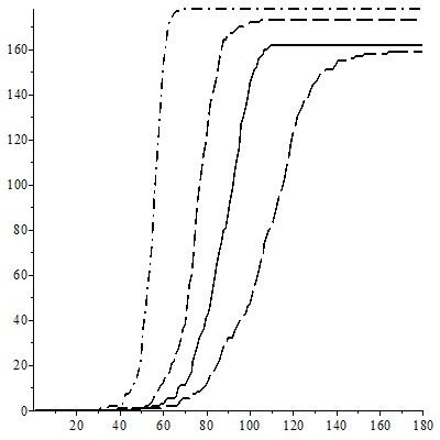
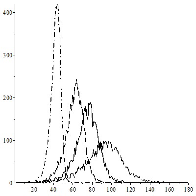
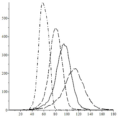
Figure 1: Evolution of the number of deceased, new individuals in H and the size of the class C when $N=10,5,4$ and $3$.

The number of deceased and the proportion of infected population are not very different between $N=4$ and $N=10$. The main difference consists in the velocity in the dissemination of the illness and so, the maximum of individuals in class C that can require hospitalization.

3.2 RQ2: How does the beginning date of the quarantine influence the spread of the disease?

Let us check the effects of a quarantine on the evolution of the disease. We assume that $N=10$ at the beginning of the spread of the disease and we consider three levels of quarantine, defined by the number of contacts $N=3$, $N=2$ or $N=0$ (the total quarantine). We can also consider what happens depending on the moment that the quarantine starts:

• when there are 10 deceased (first 10 individuals in class D),

• when there is the first deceased (first individual in class D),

• when there is the first individual with severe symptoms (first time the class C in not empty).

3.2.1 Quarantine beginning after first 10 deceased.

Let us recall that we assume that before the quarantine $N=10$. We get

Table 2: Influence of a quarantine of N at 10 deaths

$N$	10	3	2	0
Class D	189.16	186.96	183.80	184.30
	(184.15,194.16)	(181.17,192.74)	(178.04,189.55)	(179.55,189.04)
Max class C	564.23	564.60	557.46	560.66
	(557.04,571.49)	(557.04,571.41)	(551.60,563.31)	(552.22,569.09)
Total class C	12007.33	12013.86	11887.86	11960.53
	(11847.58,12167.07)	(11828.88,12198.83)	(11775.82,11999.89)	(11823.23,12097.82)
Max new H	441.16	439.73	440.66	441.90
	(432.16,449.38)	(431.53,447.92)	(434.07,447.24)	(435.30,448.49)
Day max new H	42.90	42.56	43.93	43
	(41.77,44.02)	(41.70,43.41)	(42.90,44.95)	(42.08,43.91)
Prop. infected	0.9999	0.9984	0.9967	0.9934
	(0.9998,0.9999)	(0.9983,9984)	(0.9965,0.9968)	(0.9933,0.9934)

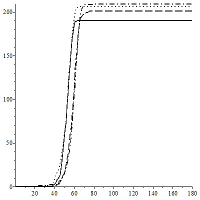
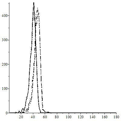
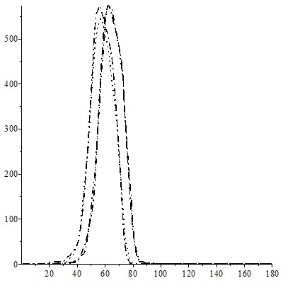
Figure 2: Evolution of the number of deceased, new individuals in H and the size of the class C when the quarantine with $N=3,2$ and $0$ begins with 10 deaths.

It is clear that the efficacy of these quarantine, including the total quarantine, is almost null, since at this level of the disease the 99% of the population has been infected (case $N=0$).

3.2.2 Quarantine beginning after the first deceased.

Table 3: Influence of a quarantine of N after the first death

$N$	10	3	2	0
Class D	189.16	174.50	157.60	105.83
	(184.15,194.16)	(168.55,180.44)	(149.26,165.93)	(89.12,122,53)
Max class C	564.23	433.23	386.80	365.40
	(557.04,571.49)	(401.39,465.06)	(339.66,433.93)	(311.49,419.37)
Total class C	12007.33	11176.66	10028.40	6860.66
	(11847.58,12167.07)	(10947.57,11405.74)	(9453.42,10603.37)	(5791.85,7929.46)
Max new H	441.16	347,50	343,06	367,73
	(432.16,449.38)	(312.17,382.82)	(299.08,387.03)	(324.30,407,15)
Day max new H	42.90	42.70	40.10	41.03
	(41.77,44.02)	(40.67,44.72)	(38.41,41.78)	(39.50,42.55)
Prop. infected	0.9999	0.9401	0.8412	0.5660
	(0.9998,0.9999)	(0.9268,0.9533)	(0.7975,0.8848)	(0.4769,0.6550)

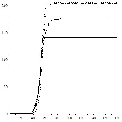
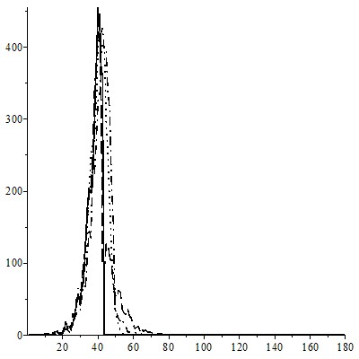
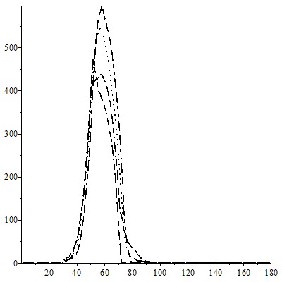
Figure 3: Evolution of the number of deceased, new individuals in H and the size of the class C when the quarantine with $N=3,2$ and $0$ begins after the first death.

In this case we can note the efficacy of a quarantine if it is rigorous, with a significant difference between $N=3$ and $N=2$. Note that in the total quarantine, there will be more that 100 deceased since at this level of the disease more of the 50% of the population has been infected (case $N=0$).

3.2.3 Quarantine beginning after the first individual enters in class C

Table 4: Influence of a quarantine of N after the first enter in C

$N$	10	3	2	0
Class D	189.16	162.80	106.70	20.96
	(184.15,194.16)	(157.16,168.43)	(98.49,114,98)	(15.51,26.40)
Max class C	564.23	272.93	130	75.50
	(557.04,571.49)	(259.34,286.51)	(104.41,155.58)	(56.90,94,09)
Total class C	12007.33	10382,53	6828,43	1337,87
	(11847.58,12167.07)	(10247.95,10517.10)	(6430.56,7226.29)	(1006.86,1668.87)
Max new H	441.16	149.36	96.96	117.13
	(432.16,449.38)	(134.02,164.69)	(68.38,125.53)	(92.21,143,04)
Day max new H	42.90	50.33	45.60	32.90
	(41.77,44.02)	(45.74,54.91)	(35.97,55.22)	(31.36,34.43)
Prop. infected	0.9999	0.8662	0.5709	0.1105
	(0.9998,0.9999)	(0.8597,0.8726)	(0.5388,0.6029)	(0.0839,0.1370)

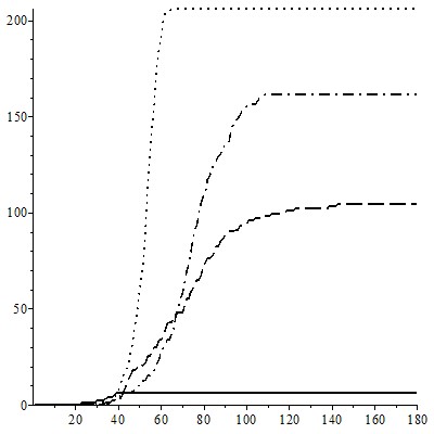
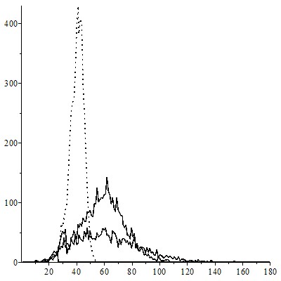
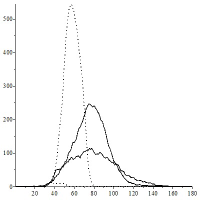
Figure 4: Evolution of the number of deceased, new individuals in H and the size of the class C when the quarantine with $N=3,2$ and $0$ begins after the first enter in C.

In this case the quarantine is effective. For $N=2$ we reduce the mortality of about 50% and for $N=0$ the number of deceased is just 20. Note that when the first individual enters in C there are about 1000 individuals infected.

3.3 RQ3: How does the duration of the quarantine influence the spread of the disease?

Let us consider now the duration of the quarantine. We consider quarantines, beginning at first individual in C, of duration 20, 60 and 120 days. We also deal with two levels of quarantine, beginning from a number of contacts of $N=10$ we pass to a quarantine with $N=3$ or $N=1$.

3.3.1 The case with $N=3$

Table 5: Influence of a quarantine (from $N=10$ to $N=3$) of duration $k$ days after the first enter in C.

$k$	0	20	60	120
Class D	189.16	186.50	172.26	160.43
	(184.15,194.16)	(181.19,191.80)	(165.68,178.83)	(155.63,165.22)
Max class C	564,23	459.96	272.23	254.50
	(557.04,571.49)	(439.43,480.48)	(256.26,288.19)	(245.09,263.90)
Total class C	12007,33	11869.33	11159.83	10319.40
	(11847.58,12167.07)	(11672.06,12066.59)	(10971.99,11349.46)	(10249.01,10389.78)
Max new H	441.16	370.5	146.73	131.03
	(432.16,449.38)	(350.32,390.67)	(133.95,159.50)	(124.94,137.11)
Day max new H	42.90	55.03	53.73	57.86
	(41.77,44.02)	(53.00,57.05)	(48.46,58.99)	(54.69,61.02)
Prop. infected	0.9999	0.9982	0.9274	0.8583
	(0.9998,0.9999)	(0.9969,0.9999)	(0.9156,0.9391)	(0.8527,0.8638)

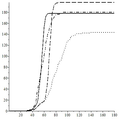
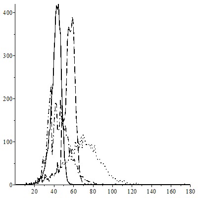
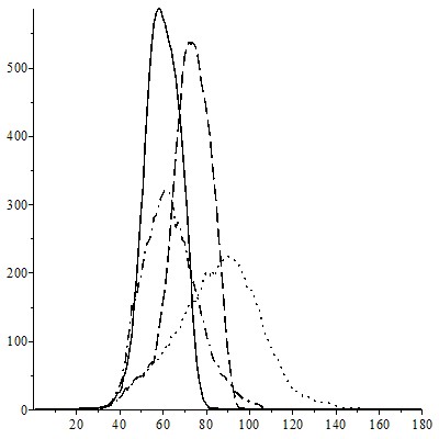
Figure 5: Evolution of the number of deaths, new individuals in H and the size of the class C when there is a quarantine of $k$ days.

When the quarantine is done with $N=3$, its effects in the number of deceased are not very important although we do a long quarantine of 120 days. Nevertheless, we are able to reduce the maximum in class C. To value the importance of the quarantine we need a more restricted quarantine.

3.3.2 The case with $N=1$

Table 6: Influence of a quarantine (from $N=10$ to $N=1$) of duration $k$ days after the first enter in C.

$k$	0	20	60	120
Class D	189.16	189.93	190.23	32.43
	(184.15,194.16)	(185.02,194.83)	(185.40,195.05)	(23.47,41.38)
Max class C	564,23	487.40	429.60	72.00
	(557.04,571.49)	(465.44,509.35)	(401.45,457.74)	(45.05,98.94)
Total class C	12007,33	12104.66	11951.36	2044.80
	(11847.58,12167.07)	(11954.15,12255.16)	(11794.90,12107.81)	(1493.54,2596.05)
Max new H	441.16	367,03	310,90	116,63
	(432.16,449.38)	(347.37,386.68)	(287.10,334.69)	(81.11,152.14)
Day max new H	42.90	66.80	113.80	56.20
	(41.77,44.02)	(65.83,67.76)	(106.08,121.51)	(36.05,76.34)
Prop. infected	0.9999	0.9993	0.9982	0.2830
	(0.9998,0.9999)	(0.9990,0.9995)	(0.9973,0.9990)	(0.2047,0.3612)

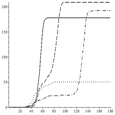
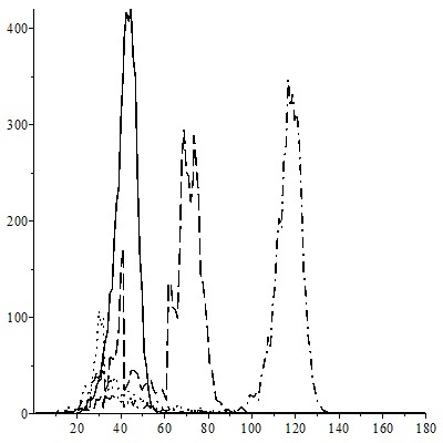
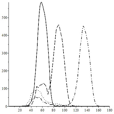
Figure 6: Evolution of the number of deaths, new individuals in H and the size of the class C when there is a quarantine of $k$ days.

We can see here that with a strong quarantine ($N=1$) and with a long quarantine ($k=120$), the disease can be stopped. In the two other cases, $k=20$ or $k=60$ the final numbers of deceased are very similar, since after a short stop the disease returns to growth up arriving at the same levels of the initial outbreak and having two clear peaks.

3.4 RQ4: How does the infectivity of asymptomatic individuals influence the spread of the disease?

One of the main problems in the study of the COVID19 disease is the role of the asymptomatic. In our general framework we have supposed that the infectivity of an asymptomatic individual (class A) is one fourth of the infectivity of an infective individual that will have symptoms (class I), that is, $q_{A}=0.05$ and $q_{I}=0.2$. Here we consider two other cases: in the first both probabilities are equal ($q_{A}=q_{I}=0.2$) and in the second case the asymptomatic individuals are not infectious ($q_{A}=0$). We also consider the case without quarantine and the case with quarantine (from $N=10$ to $N=3$) after the first individual in class C.

3.4.1 The asymptomatics’ role without quarantine

Table 7: Influence of $q_{A}$ without quarantine

$q_{A}$	0	0.05	0.2
Class D	170.93	189.16	193.13
	(153.62,188.16)	(184.15,194.16)	(187.07,199,18)
Max class C	458.66	564.23	607.76
	(412.98,504.33)	(557.04,571.49)	(599.55,615.96)
Total class C	11061.66	12007.33	11997.86
	(9967.41,12155.90)	(11847.58,12167.07)	(11834.69,12161.02)
Max new H	302,73	441.16	642,76
	(272.29,333.16)	(432.16,449.38)	(631.81,653.70)
Day max new H	52.76	42.90	35.26
	(49.07,56.44)	(41.77,44.02)	(34.63,35.88)
Prop. infected	0.9094	0.9999	1.0000
	(0.8209,0.9978)	(0.9998,0.9999)	1.0000

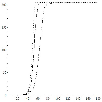
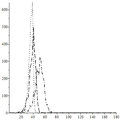
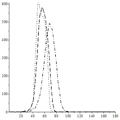
Figure 7: Evolution of the number of deaths, new individuals in H and the size of the class C with different $q_{A}$ without quarantine.

We can see that the behaviour of the disease is very similar in the three cases and the main difference just consists in the velocity of its spread.

3.4.2 The asymptomatics’ role with quarantine

Table 8: Influence of $q_{A}$ with quarantine

$q_{A}$	0	0.05	0.2
Class D	25.70	162.80	186.83
	(19.43,31.96)	(157.16,168.43)	(181.99,191.66)
Max class C	39.00	272.93	537.93
	(27.88,50.11)	(259.34,286.51)	(528.23,547.62)
Total class C	1504.93	10382.53	11967.33
	(1102.08,1907.05)	(10247.95,10517.10)	(11834.69,12161.02)
Max new H	132.43	149.36	452.33
	(116.75,148.10)	(134.02,164.69)	(409.95,494.70)
Day max new H	33.16	50.33	36.53
	(30.62,35.69)	(45.74,54.91)	(35.03,38.02)
Prop. infected	0.1353	0.8662	0.9990
	(0.1050,0.1655)	(0.8597,0.8726)	(0.9979,1)

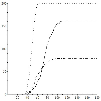
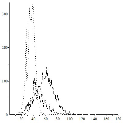
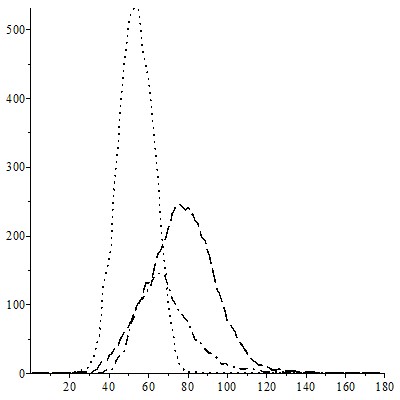
Figure 8: Evolution of the number of deaths, new individuals in H and the size of the class C with different $q_{A}$ with quarantine.

We can see the importance of knowing the role of asymptomatics in implementing quarantine. The more infectious the asymptomatic are, the more effective the quarantine is.

3.5 RQ5: How does the group immunity influence the spread of the disease?

We consider finally the group immunity. We consider three cases, where the immunity group is of 50%, 70% and 90%, respectively. We can see that an immunity of the 50% is not enough to control the disease since almost all the individuals without immunity become infected after the 180 days.

On the other hand, with an immunity of the 70% the disease is well controlled. Moreover if the immunity regards the 70% of the population, in 11 over 30 trials there aren’t any deaths and in one of the trials the disease does not infect any person.

Table 9: Influence of group immunity

Level	0%	50%	70%
Class D	189.16	90.53	18.00
	(184.15,194.16)	(87.07,93.98)	(12.78,23.21)
Max class C	564,23	207.63	20.96
	(557.04,571.49)	(202.28,212)	(14.95,26.96)
Total class C	12007.33	5804.80	1124.06
	(11847.58,12167.07)	(5680.10,5929.49)	(797.15,1450.96)
Max new H	441.16	120.76	12.40
	(432.16,449.38)	(118.41,123.10)	(9.06,15.73)
Day max new H	42.90	61.30	94.26
	(41.77,44.02)	(58.94,63.65)	(77.36,111.19)
Prop. infected	0.9999	0.4848	0.0990
	(0.9998,0.9999)	(0.4842,0.4853)	(0.0713,0.1266)

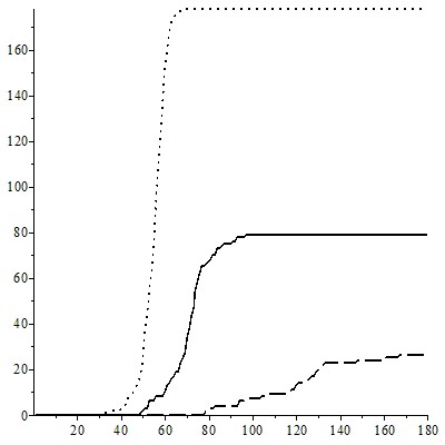
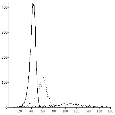
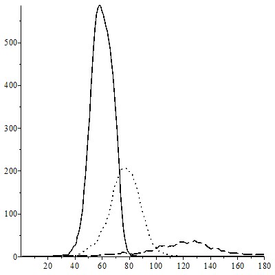
Figure 9: Evolution of the number of deaths, new individuals in H and the size of the class C when there is group immunity.

If we consider an immunity of the 90% only in 8 of the 30 trials there have been infected people with a maximum of 12 individuals infected and no one deceased.

4 Conclusions

Like any mathematical model, the model presented in this paper does not exactly describe COVID19 disease, even if it shares with this most of its characteristic. Furthermore, for this new disease many aspects are still unknown, such as the level of infectivity of asymptomatic patients.

Our goal is to understand how a disease similar to the COVID19 spreads over in a closed population and to answer to some specific research questions. What we have obtained can be summarized as follows:

1. Reducing the number of contacts of each individual the spread of the disease slows down, the pressure on the health system reduces, but we end up with a similar number of deceased.

2. It is basic to start the quarantine at least when the first severe patient is detected. Waiting for the first deceased leads to many more additional deceased.

3. To raise the quarantine it is very important to know the level of infectivity of the asymptomatic. The more infectious they are, the more important is the quarantine.

4. To stop the disease you must perform a strict and long quarantine and you must start this as soon as possible.

5. Group immunity is very important to prevent the development of the disease.

Even if most of the answers are the expected ones, we have obtained these through a sound stochastic epidemic model, that despite of its simplicity probably is able to catch most of the peculiarity of this disease.

We believe that a more sophisticated version of this model and more elaborated simulations can allow us to answer to more complex questions, but probably it will be better to wait when a deeper knowledge on this disease will be available.

References

- [1] Allen LJS (2003) An introduction to stochastic processes with applications to biology. Prentice-Hall, Englewood Cliffs.
- [2] Anderson RM, May RM (1991) Infectious Diseases of Humans. Dynamics and Control. Oxford University Press, Oxford.
- [3] Bailey NT (1975) The mathematical theory of infectious diseases and its applications. Charles Griffin & company limited, London.
- [4] Daley DJ, Gani J (1999) Epidemic modelling: an introduction. Cambridge University Press, Cambridge.
- [5] Diekmann O, Heesterbeek H, Britton T (2013) Mathematical tools for understanding infectious disease dynamics. Princeton University Press, Princeton.
- [6] Diekmann O, Heesterbeek JAP, Metz JAJ (1990) On the definition and the computation of the basic reproduction ratio R0 in models for infectious diseases in heterogeneous populations. J. Math. Biol. 28: 365?-382.
- [7] Ferrante M, Ferraris E, Rovira C, (2016) On a stochastic epidemic SEIHR model and its diffusion approximation. Test 25: 482–502.
- [8] Huang G, Takeuchi Y, Ma W, Wei D (2010) Global stability for delay SIR and SEIR epidemic models with nonlinear incidence rate. Bull. Math. Biol. 72: 1192–1207.
- [9] Kermack W, McKendrick A (1927) A contribution to the mathematical theory of epidemics. Proceedings of the Royal Society of London 115: 700–721. differential equations with time delay. Math. Comput. Simulat. 54: 189–205.
- [10] McCluskey C (2009) Global stability for an SEIR epidemiological model with varying infectivity and infinite delay. Math. Biosci. Eng. 6: 603–610.
- [11] Mode C, Sleeman C (2000) Stochastic processes in epidemiology: HIV/AIDS, other infectious diseases and computers. World Sci., Singapore.
- [12] Oli MK, Venkataraman M, Klein PA, Wendland LD, Brown MB (2006) Population dynamics of infectious diseases: A discrete time model. Ecological Modelling 198: 183–194.
- [13] Tuckwell HC, Williams RJ (2007) Some properties of a simple stochastic epidemic model of SIR type. Math. Biosci. 208: 76–97.