$\Gamma$–limit for two–dimensional charged magnetic zigzag domain walls

Abstract.

Charged domain walls are a type of domain walls in thin ferromagnetic films which appear due to global topological constraints. The non–dimensionalized micromagnetic energy for a uniaxial thin ferromagnetic film with in–plane magnetization $m\in\mathbb{S}^{1}$ is given by

$$E_{\epsilon}[m]\ =\ \epsilon\|\nabla m\|_{L^{2}}^{2}+\frac{1}{\epsilon}\|m\cdot e_{2}\|_{L^{2}}^{2}+\frac{\pi\lambda}{2|\ln\epsilon|}\|\nabla\cdot(m-M)\|_{\dot{H}^{-\frac{1}{2}}}^{2},$$ (1)

where $M$ is an arbitrary fixed background field to ensure global neutrality of magnetic charges. We consider a material in the form a thin strip and enforce a charged domain wall by suitable boundary conditions on $m$. In the limit $\epsilon\to 0$ and for fixed $\lambda>0$, corresponding to the macroscopic limit, we show that the energy $\Gamma$–converges to a limit energy where jump discontinuities of the magnetization are penalized anisotropically. In particular, in the subcritical regime $\lambda\leq 1$ one–dimensional charged domain walls are favorable, in the supercritical regime $\lambda>1$ the limit model allows for zigzaging two–dimensional domain walls.

1. Introduction and statement of main results

Magnetic domain walls are transition layers in ferromagnetic samples where the magnetization vector rapidly rotates and transitions between two regions with almost constant magnetization. A type of transition layer which is observed in thin ferromagnetic films with uniaxial in–plane anisotropy are the so-called zigzag walls (e.g. [16, 27]). These walls carry a global charge, usually necessitated by global topological constraints [22, 14]. The competition between the magnetostatic energy and other more local effects leads to the formation of two–dimensional zigzag structures as in Fig. 1. In this work, we derive a macroscopic limit for a model for zigzag walls in the framework of $\Gamma$–convergence. In the limit, the jump discontinuity is penalized by an effective anisotropic line energy.

Although it is known that two–dimensional transition layers may appear for systems with vectorial phase function, we are only aware of few analytical results on such systems [12, 17, 40, 3, 41]. The structure and energy of a charged domain wall in a one-dimensional setting has been considered by Hubert [21] on the basis of a specific ansatz function. The structure of the zigzag wall has been experimentally and numerically investigated e.g. in [16, 20, 9, 43, 27]. In particular, the angle of the zigzag structure and its dependence on temperature and thickness of the magnetic films have been studied in [27, 16]. The dynamics of the zigzag walls have been investigated numerically in [20, 9, 43, 27]. It has been observed in [42] that the zigzag wall consists of a combination of Bloch wall core and a logarithmic Néel wall tail.

Setting. In order to state our results more precisely, we present the set-up for our model: We consider a two-dimensional model for thin ferromagnetic films with uniaxial in-plane anisotropy for a magnetic sample in the form of an infinite strip $Q_{\ell}:=\mathbb{R}\times{\mathbb{T}}_{\ell}$, where ${\mathbb{T}}_{\ell}=\mathbb{R}/\ell\mathbb{Z}$ is the one-dimensional torus of length $\ell$ which is assumed to be large. The periodicity assumption in $x_{2}$–direction is purely technical, and the choice of $\ell$ does not affect our results. We enforce a charged transition layer by assuming that the magnetization $m\in H_{\rm loc}^{1}(Q_{\ell};{\mathbb{S}}^{1})$ satisfies the boundary conditions

$$m\ =\ \pm e_{1}\qquad\qquad\text{for $\pm x_{1}\ >\ 1$}.$$ (2)

The boundary condition (2) imposes a wall with transition angle of $\pi$ (modulo $2\pi$). Also by (2), the total charge is $\int\nabla\cdot m\ dx=2\ell\neq 0$, where we recall that $\nabla\cdot m$ is the magnetic charge density associated with $m$. The energy for this problem is given by

$$\begin{aligned} E_{\epsilon}[m]\ &=\ \frac{1}{2}\int_{Q_{\ell}}\epsilon|\nabla m|^{2}\ dx+\frac{1}{2}\int_{Q_{\ell}}\frac{1}{\epsilon}|m\cdot e_{2}|^{2}\ dx\\ &\qquad\qquad+\frac{\pi\lambda}{2|\ln\epsilon|}\int_{Q_{\ell}}\big{|}|\nabla|^{-\frac{1}{2}}\nabla\cdot(m-M)\big{|}^{2}\ dx\end{aligned}$$ (3)

for some fixed background magnetization $M\in C^{1}(Q_{\ell};{\mathbb{S}}^{1})$ with $\operatorname*{spt}(DM)\Subset Q_{\ell}$, which is chosen such that the system is charge-free, i.e.

$$\int_{{Q_{\ell}}}\nabla\cdot(m-M)\ dx\ =\ 0$$ (4)

(the fractional Sobolev norm in (3) is defined in (14)). We note that the background magnetization is needed to allow for states with finite energy and that our results do not depend on the specific choice of $M$ (a possible choice is the transition layer in Lemma 3.3 with $\epsilon=\beta=1$). The components of the energy in order are called exchange energy, anisotropy energy and stray field energy. The small parameter $\epsilon>0$ describes the relative size of the transition layer with respect to the width of the strip. The material parameter $\lambda\geq 0$, describes the relative strength of the stray field and anisotropy energy (for a derivation see Section 1.2).

The class of admissible functions ${\mathcal{A}}$ for the energy (3) is given by

$${\mathcal{A}}\ =\ \big{\{}m\in H^{1}_{\textrm{loc}}(Q_{\ell};{\mathbb{S}}^{1})\ :\ \text{$m$ satisfies \eqref{bc}}\big{\}}.$$ (5)

We extend $E_{\epsilon}$ to a functional on the affine space $M+L^{1}(Q_{\ell};\mathbb{R}^{2})$ by setting $E_{\epsilon}[m]:=+\infty$ for $m\not\in{\mathcal{A}}$. We note that the space does not depend on the specific choice of $M$ above.

The transition layer we consider is called a charged domain wall, since by the boundary condition the magnetization $m$ has a net charge $\int\nabla\cdot m\ dx\neq 0$ as explained above. In contrast, transition layers where the total net charge vanishes are called charge-free (cf. [22]). Transition layers in thin films with in–plane rotation, as considered in this work, of the magnetization are also called Néel walls.

Main result and discussion. The main result in this paper is the derivation of an effective model for the energy (3) in the macroscopic limit $\epsilon\to 0$ for any fixed $\lambda\geq 0$. In this limit, both the local and the nonlocal part of the energy concentrate on the one-dimensional jump set of the magnetization. Moreover, the stray field energy yields an anisotropic contribution to the penalization of the jump discontinuity:

Theorem 1.1 ($\Gamma$–convergence).

Let $\lambda\geq 0$. For any sequence $m_{\epsilon}\in{\mathcal{A}}$, $\epsilon\to 0$, with

$$\limsup_{\epsilon>0}E_{\epsilon}[m_{\epsilon}]\ \leq\ K\ <\infty$$ (6)

there is a subsequence $\epsilon_{k}\to 0$ with $m_{\epsilon_{k}}\to m_{0}$ in $L^{1}$ for some $m_{0}\in{\mathcal{A}}_{0}$ as $k\to\infty$, where ${\mathcal{A}}_{0}$ $=$ $\{$ $m\in BV_{\textrm{loc}}(Q_{\ell};\{\pm e_{1}\})$ : $m$ satisfies (2) $\}$. Furthermore, the energies $E_{\epsilon}$ $\Gamma$–converge to $E_{0}$ in the $L^{1}$-topology, where

$$E_{0}[m]=\displaystyle 2\int_{\SS_{m}}\left(1+\lambda|e_{1}\cdot n|^{2}\right)\chi_{\{|e_{1}\cdot n|\leq\frac{1}{\sqrt{\lambda}}\}}+2\sqrt{\lambda}|e_{1}\cdot n|\chi_{\{|e_{1}\cdot n|>\frac{1}{\sqrt{\lambda}}\}}\ d{\mathcal{H}}^{1}\quad$$ (7)

if $m\in{\mathcal{A}}_{0}$ and $E_{0}[m]=+\infty$ otherwise for $m\in M+L^{1}(Q_{\ell};\mathbb{R}^{2})$. Here, $\SS_{m}$ is the jump set of $m$ with the measure theoretic unit normal $n$. In particular,

1. For any sequence $m_{\epsilon}\in{\mathcal{A}}$ with $m_{\epsilon}\to m\in{\mathcal{A}}_{0}$ in $L^{1}$ we have

   $$\liminf_{\epsilon>0}E_{\epsilon}[m_{\epsilon}]\ \geq\ E_{0}[m].$$ (8)

2. For any $m\in{\mathcal{A}}_{0}$, there is a sequence $m_{\epsilon}\in{\mathcal{A}}$ with $m_{\epsilon}\to m$ in $L^{1}$ and

   $$\limsup_{\epsilon>0}E_{\epsilon}[m_{\epsilon}]\ \leq\ E_{0}[m].$$ (9)

It is well–known that the exchange energy and anisotropy energy together asymptotically lead to an isotropic penalization of the length of the jump set $\SS_{m}$ [5]. However, in our model the presence of the magnetostatic energy yields an additional penalization for the jump discontinuity contributing to the limit energy, which depends on the line charge density given by the jump of the normal derivative of $m$ over the jump set $\SS_{m}$ ($=2|n\cdot e_{1}|$ in our setting). We note that both the local terms and the nonlocal stray-field energy contribute to the limit energy in leading order.

The minimal energy for given $\lambda\geq 0$ for the limit problem is

$$e(\lambda)\ :=\ \min_{m\in{\mathcal{A}}_{0}}E_{0}[m]\ =\ 2\ell\begin{cases}1+\lambda\qquad&\text{ for }\lambda\leq 1,\\ 2\sqrt{\lambda}&\text{ for }\lambda>1\end{cases}$$ (10)

(see Proposition 4.1). The crossover at the critical value $\lambda=1$ in (10) signifies that zigzag configurations are energetically preferable on the $\epsilon>0$ level for $\lambda>1$ but not for $\lambda\leq 1$, when the isotropic part of the limit energy dominates. Correspondingly, minimizers for the limit energy are degenerate for $\lambda>1$: In this case any jump set $\SS_{m}$ which can be written as a graph in $x_{2}$ and with measure theoretic normal $n$ satisfying $|n\cdot e_{1}|\geq\lambda^{-\frac{1}{2}}$ is a global minimizer of the energy, see Fig. 1b). In particular, for $\lambda>1$ the set of minimizers of the limit problem includes zigzag configurations. For $\epsilon>0$, these minimizers can be approximated by zigzag–shaped transition layers with normal satisfying $|n\cdot e_{1}|=\lambda^{-\frac{1}{2}}$ and with rapid oscillation in tangential direction (Lemma 3.1).

a)   b)

Figure 1. a) Experimental picture of zigzag wall separating antiparallel domains [22, Fig. 5.61] b) Different global minimizers for the limit energy in the supercritical case. For all minimizers, the normal of the jump set satisfies $|n\cdot e_{1}|\geq\lambda^{-\frac{1}{2}}$.

Transition layers between two phases are usually one–dimensional — such as e.g. for Ginzburg–Landau type energies and the Aviles-Giga energy [15]. While it is known that transition layers for models with vectorial phase field function might be two–dimensional, only few analytical results exist for this case. In particular, we are not aware of another analytical result for a thin–film micromagnetic energy as in (3). Two–dimensional structures for related micromagnetic energies are investigated for the cross–tie wall by Alouges, Rivière and Serfaty in [3, 41] and for a zigzag transition layer by Moser in [38] and by Ignat and Moser in [24]. In these works, a setting is considered where the magnetization is constant in one coordinate direction and where the nonlocal energy is given by the square of the $H^{-1}$–norm (relevant for bulk materials). In particular, Ignat and Moser [24] consider non–charged transition layers for a prescribed transition angle and derive a $\Gamma$–limit for the energy in the macroscopic regime $\epsilon\to 0$ and based on the weak^∗ $L^{\infty}$–topology. In this situation, the strong penalization of the stray field energy enforces divergence free configurations in the limit and leads to zigzag configurations for small transition angles. Different from our situation, the nonlocal energy does not contribute to the limit energy. The proof in [24] is based on the entropy method. Since we consider the critical $\frac{1}{|\ln\epsilon|}$ scaling of the nonlocal terms which allows for charged walls in the limit and where the nonlocal energy contributes to the limit energy (different from [24]), the entropy method does not seem to apply to our model.

For thin films, charge–free transition layers with a $\pi$ transition angle (of Néel wall type) have been investigated e.g. in [36, 37, 25, 23]. In particular, in [13], DeSimone, Otto and the first author show that for the charge–free Néel wall, one–dimensional transition layers are asymptotically energetically optimal. This explains why zigzag type transition layers do not appear for charge–free Néel wall domain walls. On the other hand, for the charged Néel wall considered in this work, the concentration of line charges leads to formation of zigzag patterns as described above. We note that both charged and charge-free Néel wall exhibit a characteristic logarithmically decaying tail [36, 37, 42]. However, the leading order contribution to the energy is carried in the tail for the charge–free Néel wall, while it is concentrated in the core for the charged Néel wall.

Our argument for the liminf inequality in the $\Gamma$-convergence is based on a duality argument and the construction of a suitable test function as in [13]. For the construction of the test function there are fundamental differences compared to the previous work, where the test function is a characteristic function constructed by a Poincaré–Bendickson argument: In particular, the test function in this work is supported in the neighborhood of a so-called separating curve with logarithmic decaying profile. In the construction of the test function, we need to develop and use some new level set estimates. The detailed strategy of our proof is described in Section 1.1.

Remark 1.2 (One–dimensional setting).

One–dimensional transition layers for (2)–(3) are also simply called charged domain walls. The energy (with $\ell=1$) then takes the form

$$\frac{1}{2}\int_{\mathbb{R}}\epsilon|\frac{dm}{dx_{1}}|^{2}+\frac{1}{\epsilon}|m\cdot e_{2}|^{2}\ dx_{1}+\frac{\pi\lambda}{2|\ln\epsilon|}\int_{\mathbb{R}}\big{|}|\frac{d}{dx_{1}}|^{\frac{1}{2}}(m-M)\cdot e_{1}\big{|}^{2}\ dx_{1}.$$ (11)

The limit energy then simply counts the number of jumps of the one–dimensional transition layer $m\in{\mathcal{A}}_{0}$, and each jump is penalized by the factor $2(1+\lambda)$. The one-dimensional energy (11) has been analyzed in [21] in terms of specific ansatz functions.

Finally, we note that the existence of minimizers for the energy for the three–dimensional micromagnetic model has been shown by Anzellotti, Baldi and Visintin in [5], and the arguments can be easily adapted to our setting. We also note that variants of the Modica-Mortola model in the presence of nonlocal interactions have been considered e.g. in [2]. The competition between interfacial and nonlocal energies also plays a role for the Ohta-Kawasaki model. We mention a few, but by far not exhaustive list of related works, in which this energy is studied in a periodic [10, 11, 19] or bounded domain [1, 28, 29, 19, 6, 26].

Notation. Throughout the paper, we denote by $C$ a positive universal constant unless specified; $\epsilon\in(0,\frac{1}{4})$ is a small parameter and $\ell\gg 1$ is a large parameter. For any set $E\subset\mathbb{R}^{2}$, we write $d_{E}(x):=\operatorname*{dist}(x,E)$ for the distance to this set, noting that the distance to the empty set is infinite. For a set $E\subset\mathbb{R}^{2}$ we write $\mathcal{N}_{t}(E):=\{x\in\mathbb{R}^{2}:d(x,E)<t\}$ for its $t$-neighborhood. The $k$–dimensional Hausdorff measure of the set $E\subset\mathbb{R}^{n}$ is denoted by ${\mathcal{H}}^{k}(E)$.

BV functions, sets of finite perimeter: Given an open subset $U\subset\mathbb{R}^{n}$, $BV_{loc}(U)$ denotes the space of functions which have locally bounded variation in $U$ (see [35] for further details). A measurable set $F\subset\mathbb{R}^{n}$ has locally finite perimeter in $U$ if the characteristic function $\chi_{F}\in BV_{loc}(U)$. We let $\|Du\|(U)$ denote the total variation measure in $U$ and $\|D\chi_{F}\|(U)$ denote the relative perimeter of $F$ in $U$. The reduced boundary $\partial^{*}F$ of $F$ is the set of points $x\in\operatorname*{spt}D\chi_{F}$ where the measure theoretic outer normal $n(x)$ exists. Any function $u\in L^{1}_{loc}(U)$ has an approximate limit for a.e. $x\in U$, i.e. $\lim_{\rho\to 0+}\fint_{B_{\rho}(x)}|u(y)-z|dy=0$ for some $z\in\mathbb{R}$. The jump set $\tilde{\SS}_{u}$ is the set of points at which the approximate limit does not exist. For $u\in BV_{loc}(U;\{\pm 1\})$, we write $\{x\in U:u(x)=1\}$ for the set of points where the approximate limit of $u$ is $1$. In this case, the jump set $\tilde{\SS}_{u}$ is ${\mathcal{H}}^{n-1}$-a.e. equal to $\SS_{u}:=\partial^{*}\{x\in U:u(x)=1\}$, the reduced boundary of this set. Furthermore, $\|Du\|(K)=2{\mathcal{H}}^{n-1}(\SS_{u}\cap K)$ for any $K\Subset U$.

Some notions for functions and sets on $Q_{\ell}=\mathbb{R}\times{\mathbb{T}}_{\ell}$: We note that there is a canonical projection $\Pi:\mathbb{R}^{2}\to Q_{\ell}$. Correspondingly, we identify functions on $Q_{\ell}$ with $Q_{\ell}$–periodic functions on $\mathbb{R}^{2}$. Similarly, any set $\Omega\subset Q_{\ell}$ can be identified with its periodic extension onto $\mathbb{R}^{2}$. For $\varphi\in L^{1}(Q_{\ell})$ we write

$$\widehat{\varphi}(\xi)\ :=\ \frac{1}{\sqrt{2\pi\ell}}\int_{Q_{\ell}}e^{i\xi\cdot x}\,\varphi(x)\,dx\qquad\qquad\text{where $\xi\in\mathbb{R}\times\frac{2\pi}{\ell}\mathbb{Z}$,}$$ (12)

i.e. we use the Fourier transformation in $x_{1}$ and the Fourier series in $x_{2}$. We will use the short notation $\int_{\mathbb{R}\times\frac{2\pi}{\ell}\mathbb{Z}}\cdot d\xi:=\ \sum_{\xi_{2}\in\frac{2\pi}{\ell}\mathbb{Z}}\int_{\mathbb{R}}\cdot d\xi_{1}$. Plancherel’s identity then takes the form

$$\int_{Q_{\ell}}\overline{\varphi(x)}\psi(x)\ dx\ =\ \int_{\mathbb{R}\times\frac{2\pi}{\ell}\mathbb{Z}}\overline{\widehat{\varphi}(\xi)}\widehat{\psi}(\xi)\ d\xi.$$ (13)

The fractional Sobolev norms on $Q_{\ell}$ for $\alpha\in\mathbb{R}$ are defined by

$$\int_{Q_{\ell}}\big{|}|\nabla|^{\alpha}\varphi\big{|}^{2}\ dx\ :=\ \int_{\mathbb{R}\times\frac{2\pi}{\ell}\mathbb{Z}}\big{|}|\xi|^{\alpha}|\widehat{\varphi}(\xi)|\big{|}^{2}\ d\xi.$$ (14)

In the appendix we give two more representations of the homogeneous $H^{\frac{1}{2}}$–norm.

1.1. Overview and strategy for the proofs

In this section, we give an overview of the proofs for our results. In particular, we describe the strategy for the proof of the liminf inequality in Theorem 1.1, which represents the main novelty in this paper. Solution for the limit problem is given in Proposition 4.1 in Section 4.

Compactness. The compactness follows by a well–known argument (see [5]). For the sequence $m_{\epsilon}=(u_{\epsilon},v_{\epsilon})\in{\mathcal{A}}$ from Theorem 1.1, we have

$$\int_{Q_{\ell}}|\nabla u_{\epsilon}|\ dx\ \leq\ \frac{1}{2}\int_{Q_{\ell}}\Big{(}\frac{\epsilon|\nabla u_{\epsilon}|^{2}}{1-u_{\epsilon}^{2}}+\frac{1-u_{\epsilon}^{2}}{\epsilon}\Big{)}\ dx\ =\ \frac{1}{2}\int_{Q_{\ell}}\Big{(}\epsilon|\nabla m_{\epsilon}|^{2}+\frac{v_{\epsilon}^{2}}{\epsilon}\Big{)}\ dx\ \leq\ K.$$ (15)

Together with the boundary conditions (2) it follows that $v_{\epsilon}\to 0$ in $L^{1}(Q_{\ell})$. After selection of a subsequence, we also have $u_{\epsilon}\to u\in BV_{\rm loc}(Q_{\ell};\{\pm 1\})$ in $L^{1}(Q_{\ell})$. Since the boundary conditions are still satisfied in the limit, we get $m_{\epsilon}\to m=(u,0)$ in $L^{1}$ for $m\in{\mathcal{A}}_{0}$.

Liminf inequality. We describe the strategy of the proof, the details are given in Section 2: We consider a sequence $m_{\epsilon}\in{\mathcal{A}}$ with $m_{\epsilon}\to m=(u,0)\in{\mathcal{A}}_{0}$ in $L^{1}$ for $\epsilon\to 0$ such that (6) holds. The jump set of $m$ (or equivalently of $u$) is ${\mathcal{H}}^{1}$ a.e. equal to $\SS_{m}:=\partial^{*}\{x\in Q_{\ell}:u(x)=1\}$. The unit outer normal of $\{x\in Q_{\ell}:u(x)=1\}$ along $\SS_{m}$ is denoted by $n$.

Step 1: Localization argument. The first step of the proof is a localization argument (see Section 2.4 for details). The idea is to choose a family of pairwise disjoint balls $B_{k}\subset Q_{\ell}$ with sufficiently small radius which almost covers $\SS_{m}$, and suitable cut-off functions $\chi_{\epsilon,k}$ with $\operatorname*{spt}\chi_{\epsilon,k}\Subset B_{k}$ and $\chi_{\epsilon,k}\to\chi_{B_{k}}$ as $\epsilon\to 0$. We write $E_{\epsilon}$ in the form

$$E_{\epsilon}[m_{\epsilon}]\ =\ \sum_{k}\Big{(}\nu_{\epsilon}(B_{k})+N_{\epsilon}[\chi_{\epsilon,k}]\Big{)}+R_{\epsilon}.$$ (16)

The two terms $\nu_{\epsilon}(B_{k})$ and $N_{\epsilon}[\chi_{\epsilon,k}]$ represent the interfacial energy in the ball $B_{k}$ and the self–interaction energy within the ball respectively, i.e.

$$\nu_{\epsilon}(B_{k})\ :=\ \frac{1}{2}\int_{B_{k}}\Big{(}\epsilon|\nabla m_{\epsilon}|^{2}+\frac{v_{\epsilon}^{2}}{\epsilon}\Big{)}\ dx,$$ (17)

$$N_{\epsilon}[\chi_{\epsilon,k}]\ :=\ \frac{\lambda}{4|\ln\epsilon|}\int\!\!\!\!\int_{\mathbb{R}^{2}\times\mathbb{R}^{2}}\frac{(\chi_{\epsilon,k}\sigma_{\epsilon})(x)(\chi_{\epsilon,k}\sigma_{\epsilon})(y)}{|x-y|}\ dxdy,$$ (18)

where $\sigma_{\epsilon}:=\nabla\cdot(m_{\epsilon}-M)$ is the magnetic charge density. Here and in the sequel with a slight abuse of notation we identify $\chi_{\epsilon,k}$ with the cut-off function associated with a single representative of the ball $B_{k}$ in $\mathbb{R}^{2}$. The remainder $R_{\epsilon}$ can be estimated from below as a lower order term if the balls are chosen carefully (cf. Proposition 2.13). Hence, the estimate is reduced to local estimates on the balls $B_{k}$.

Step 2: Local estimate of leading order terms. We claim that for any ball $B:=B_{k}$ and corresponding cut–off function $\chi_{\epsilon}:=\chi_{\epsilon,k}$ with $\operatorname*{spt}\chi_{\epsilon}\Subset B$, we have

$$\liminf_{\epsilon\to 0}\ \Big{(}\nu_{\epsilon}(B)+N_{\epsilon}[\chi_{\epsilon}]\Big{)}\ \geq\ 2\int_{\SS_{m}\cap B}f(\sqrt{\lambda}|n\cdot e_{1}|)\ d{\mathcal{H}}^{1},$$ (19)

where $f$ is the energy density of the limit functional, i.e.

$$f(s)\ :=\ \left(1+s^{2}\right)\chi_{\{s\leq 1\}}+2s\chi_{\{s>1\}}\ =\ \inf_{\alpha\geq 1}\Big{[}\alpha+\frac{s^{2}}{\alpha}\Big{]}\ \qquad\text{for $s>0$.}$$ (20)

The lower bound is determined by a balance between interfacial and magnetostatic terms: We first note that by (15) and the lower semi-continuity of the BV norm, we have

$$\liminf_{\epsilon\to 0}\nu_{\epsilon}(B)\ \geq\ \liminf_{\epsilon\to 0}\|Du_{\epsilon}\|(B)\ =:\ \alpha\|Du\|(B)$$ (21)

for some $\alpha\geq 1$, where the difference $\alpha-1\geq 0$ quantifies the local presence of oscillations as $\epsilon\to 0$. In view of the second identity in (20), it is then enough to show that

$$\liminf_{\epsilon\to 0}N_{\epsilon}[\chi_{\epsilon}]\ \geq\ \frac{2\lambda}{\alpha}\int_{\SS_{m}\cap B}|n\cdot e_{1}|^{2}\ d{\mathcal{H}}^{1}.$$ (22)

Step 3: Estimate of main nonlocal term. For the estimate of (22), we first note that

$$N_{\epsilon}[\chi_{\epsilon}]=\frac{\pi\lambda}{2|\ln\epsilon|}\int_{\mathbb{R}^{2}}\big{|}|\nabla|^{-\frac{1}{2}}(\chi_{\epsilon}\sigma_{\epsilon})\big{|}^{2}\ dx.$$ (23)

Then we use the dual characterization of the $\dot{H}^{-\frac{1}{2}}(\mathbb{R}^{2})$– norm, i.e. we use that for any $\Phi\in\dot{H}^{\frac{1}{2}}(\mathbb{R}^{2})$ we have

$$\int_{\mathbb{R}^{2}}\chi_{\epsilon}^{2}\sigma_{\epsilon}\Phi\ dx\ \leq\ \Big{(}\int_{\mathbb{R}^{2}}\big{|}|\nabla|^{-\frac{1}{2}}(\chi_{\epsilon}\sigma_{\epsilon})\big{|}^{2}\ dx\Big{)}^{\frac{1}{2}}\Big{(}\int_{\mathbb{R}^{2}}||\nabla|^{\frac{1}{2}}(\chi_{\epsilon}\Phi)|^{2}\ dx\Big{)}^{\frac{1}{2}}.$$ (24)

For the construction of the test functions, we choose a cut-off function $\eta_{\epsilon}\in C_{c}^{\infty}(\mathbb{R})$ with logarithmically decaying profile (see Definition 2.6). The functions $\Phi_{\epsilon}$ have the form

$$\Phi_{\epsilon}(x)\ :=\ \eta_{\epsilon}(\operatorname*{dist}{(\gamma_{\epsilon},x)}),$$ (25)

where $\gamma_{\epsilon}$ are carefully modified level sets $\{u_{\epsilon}=t\}$ in $B_{k}$ with certain $t$ such that in particular the following properties hold:

1. For each $\epsilon>0$, the set $\gamma_{\epsilon}$ separates the regions where $m_{\epsilon}\approx e_{1}$ and $m_{\epsilon}\approx-e_{1}$ (up to small sets) and converges to $\SS_{m}$ in a weak sense as $\epsilon\to 0$. Furthermore, the sets $\gamma_{\epsilon}$ have uniformly controlled length.

2. the length of level sets of certain distance from $\gamma_{\epsilon}$ is controlled, i.e. ${\mathcal{H}}^{1}(d_{\gamma_{\epsilon}}^{-1}(t)\cap B)\leq 2{\mathcal{H}}^{1}(\gamma_{\epsilon})$ for a.e. $t\in(0,\delta_{0})$ and some $\delta_{0}>0$.

The precise statements and the details of the construction are given in Sections 2.2 and 2.1 (see Lemma 2.5). To construct the sets $\gamma_{\epsilon}$ such that they satisfy (i) it would be enough to choose them as suitably chosen level sets of $u_{\epsilon}$. To achieve (ii) we modify $\gamma_{\epsilon}$, and we use and adapt the level sets estimates from [7], which are based on the Gauss–Bonnet theorem and rely crucially on the two–dimensionality of our problem.

Estimate (22) then follows by deriving sharp estimates for the terms in (24), i.e.

$$\int_{\mathbb{R}^{2}}\big{|}|\nabla|^{\frac{1}{2}}(\chi_{\epsilon}\Phi_{\epsilon})\big{|}^{2}\ dx\ \leq\ \Big{(}\frac{\pi}{|\ln{\epsilon}|}+o(\frac{1}{|\ln\epsilon|})\Big{)}{\mathcal{H}}^{1}(\gamma_{\epsilon}),$$ (26)

$$\int_{\mathbb{R}^{2}}\chi_{\epsilon}^{2}\Phi_{\epsilon}\sigma_{\epsilon}\ dx\ \geq\ 2\int_{\SS_{m}}\chi_{\epsilon}^{2}(n_{\epsilon}\cdot e_{1})\ d{\mathcal{H}}^{1}-o(1)$$ (27)

for $\epsilon\to 0$. It is essential that we get the precise leading order constant in both (26)–(27). We note that (26) means that the capacity of the curves $\gamma_{\epsilon}$ is asymptotically controlled by their length, where we recall that the capacity of a set is the reciprocal of the minimal stray field energy created by a charge distribution with total charge one on the set (cf. e.g. [33]). Thus the assertion (ii) is the right estimate for the derivation of (26).

Limsup inequality. The limsup inequality follows by constructing a suitable recovery sequence. This recovery sequence is constructed by patching one–dimensional transition layers together. Additional care is taken in the supercritical case, where we replace transition layers with large slopes by fine combination of suitable zigzags. The estimate of the stray field energy relies on the singular integral representation for the $\dot{H}^{-\frac{1}{2}}$-norm (cf. Lemma A.3). Using this representation, we can localize the self–interaction term to each patch which yields the leading order contribution of the energy. It can be furthermore shown that the interaction energy between different patches is of lower order. The construction and estimates for the recovery sequence are given in Section 3.

1.2. Formal derivation of the model

Before we give the proofs of the main results, we show how the model (3)–(4) can be derived from a non-dimensionalization of the underlying three-dimensional physical model [32] (for similar arguments see e.g. [18, 36]). We apply some heuristic simplifications which we believe can be justified rigorously.

We consider a uniaxial ferromagnetic in the shape of a thin plate of the form $\Omega=\mathbb{R}^{2}\times[0,t]$ and magnetization $\overline{m}=(m,m_{3}):\mathbb{R}^{2}\times[0,t]\to\mathbb{S}^{2}$. The single, energetically preferred magnetization direction of the material in consideration is given by the $e_{1}$–axis. Since we are interested in a charged transition layer, we enforce this transition by boundary conditions, i.e. we assume $\overline{m}=\pm e_{1}$ for $\pm x_{1}>w$ for some $w>0$. In order to formulate the problem, we assume that $\overline{m}$ is $L$–periodic in $x_{2}$ direction for some large periodicity $L$, noting that our estimates do not depend on $L$. Let $Q_{L}:=\mathbb{R}\times{\mathbb{T}}_{L}$, where ${\mathbb{T}}_{L}:=\mathbb{R}/(L\mathbb{Z})$. As described before, we assume that there is a background magnetization $\overline{M}$ which ensures that the system is charge free, i.e. the analogous assumption to (4) holds. Physically, this corresponds to the fact that there are no magnetic monopoles. In a partially non–dimensionalized form, the Landau-Lifshitz energy [32, 15] then takes the form

$$\begin{aligned} {\mathcal{E}}[\overline{m}]&=\ d^{2}\int_{Q_{L}\times(0,t)}|\overline{\nabla}\overline{m}|^{2}\ d\overline{x}+Q\int_{Q_{L}\times(0,t)}(m_{2}^{2}+m_{3}^{2})\ d\overline{x}+\int_{Q_{L}\times\mathbb{R}}|\overline{h}|^{2}\ d\overline{x},\end{aligned}$$ (28)

with the notation $\overline{x}=(x,x_{3})$ and $\overline{\nabla}=(\nabla,\partial_{3})$. Here, the material parameter $d$ is the so called exchange length, modelling the relative strength of the exchange and magnetostatic or stray field energy. The dimensionless constant $Q>0$ is the quality factor, which describes the relative strength of the material anisotropy. The stray field $\overline{h}\in L^{2}(Q_{L}\times\mathbb{R};\mathbb{R}^{3})$ is given by $\overline{h}\ :=\ \overline{\nabla}(-\Delta_{Q_{L}\times\mathbb{R}})^{-1}\overline{\nabla}\cdot(\overline{m}-\overline{M})$, which is the Helmholtz projection of $\overline{m}-\overline{M}$ on the gradient fields. If the magnetic film is sufficiently thin, it is reasonable to assume that the magnetization does not vary in the thickness direction within the film. In this case, the stray field equations can be solved explicitly, cf. [14]. Also assuming that $m$ varies on length scales much larger than $t$ we can apply a standard low frequency approximation for the stray field energy (see e.g. [8, 31]). With the change of variables $\overline{x}\mapsto\frac{\overline{x}}{w}$, denoting $\ell:=\frac{L}{w}$, we arrive at the reduced energy

$$\begin{aligned} {\mathcal{E}}_{\textrm{red}}[\overline{m}]\ &=\ d^{2}t\int_{Q_{\ell}}|\nabla\overline{m}|^{2}\ dx+Qtw^{2}\int_{Q_{\ell}}(m_{2}^{2}+m_{3}^{2})\ dx+tw^{2}\int_{Q_{\ell}}m_{3}^{2}\ dx\\ &\qquad+\ \frac{t^{2}w}{2}\int_{Q_{\ell}}\big{|}|\nabla|^{-\frac{1}{2}}\nabla\cdot(m-M)\big{|}^{2}\ dx\end{aligned}$$ (29)

for $m\in{\mathcal{A}}$. We introduce the dimensionless parameters $\epsilon$, $\lambda$, and $\alpha$ by

$$\epsilon\ :=\ \frac{d}{wQ^{\frac{1}{2}}},\qquad\lambda\ :=\ \frac{t|\ln\epsilon|}{2\pi dQ^{\frac{1}{2}}},\qquad\alpha\ :=\ \frac{w}{t}.$$ (30)

Note that $\epsilon$ represents the ratio of Bloch wall width and sample width $w$ [14]. The parameter $\lambda$ is related to the relative strength of the stray field energy for the charged Néel wall to the local energy (cf. (3)). The parameter $\alpha$ describes the aspect ratio. Rescaling the energy, we arrive at

$$\frac{{\mathcal{E}}_{\textrm{red}}[\overline{m}]}{2dtwQ^{\frac{1}{2}}\ell}\ =\ E_{\epsilon}[m]\ +\Big{(}\frac{1}{\epsilon}+\frac{\pi\lambda\alpha}{2|\ln\epsilon|}\Big{)}\int_{Q_{\ell}}m_{3}^{2}\ dx.$$ (31)

For sufficiently thin films we have $\alpha\gg\frac{1}{\epsilon}|\ln\epsilon|$ and the out–of–plane component of the magnetization is penalized heavily. This suggests to assume $m_{3}=0$, and we arrive at the form (3) for the non–dimensionalized energy.

Remark 1.3 (Statement of results in initial variables).

The $\Gamma$–limit in Theorem 1.1 corresponds to the following scaling of the initial energy: In the regime $t\ll d$, $d^{2}\ \ll\ wt$ and $Q^{\frac{1}{2}}\ \approx\ \frac{t}{2\pi\lambda d}|\ln(\frac{d^{2}}{wt})|$, the ground state energy in leading order is given by

$$\min_{\overline{m}}{\mathcal{E}}[\overline{m}]\ \approx\ t^{2}L\big{|}\ln\big{(}\frac{d^{2}}{wt}\big{)}\big{|}\begin{cases}\displaystyle\left(1+\lambda\right)\qquad&\text{ if }\lambda\leq 1,\vspace{0.7ex}\\ \displaystyle\sqrt{4\lambda}&\text{ if }\lambda>1,\end{cases}$$ (32)

where the minimum is taken over all configurations $\overline{m}\in H^{1}(Q_{L};\mathbb{S}^{2})$ with $\overline{m}=\pm e_{1}$ for $\pm x_{1}>w$. In order to get a corresponding $\Gamma$–limit for the full energy (28) and to rigorously prove (32), it is necessary to show that the assumptions made in this section only lead to errors which are negligible with respect to the leading order terms in the energy.

2. Proof of Theorem 1.1 – liminf–inequality

2.1. Level set estimates

In this section, we give some general results for the length of level sets for the distance function to the boundary of sets $\Omega\subset\mathbb{R}^{2}$. These results are used in the construction of our test function in the proof of Lemma 2.5, which then is used in the proof of the liminf–inequality. The main result is Theorem 2.3, which shows that we can modify a set locally such that the boundary of the new set has a controlled capacity. The key in the proofs is an application of the Gauss-Bonnet theorem. The proofs also rely heavily on the two–dimensionality of the problem.

We first consider the situation of bounded simply connected domains $G$ before addressing more general sets. The proof of the next lemma follows from the ideas in [7, Lemma 3.2.2-3.2.3]. We note that Lemma 3.2.2 in [7] is stated for inner level sets, i.e. level sets for $d_{\partial E}$ inside $E$. However, it is not hard to see that it holds for outer level sets as well. For any set $E\subset\mathbb{R}^{2}$, we write $d_{E}(x):=\operatorname*{dist}(x,E)$ for the distance to this set, noting that the distance to the empty set is infinite.

Lemma 2.1 (Level sets of simply connected domains).

For any bounded simply connected domain $G\subset\mathbb{R}^{2}$ with piecewise $C^{2}$ boundary, we have

$${\mathcal{H}}^{1}(d_{\partial G}^{-1}(t))\ \leq\ 2{\mathcal{H}}^{1}(\partial G)\qquad\quad\quad\text{for a.e. $0\ \leq t\leq\ \frac{1}{2\pi}{\mathcal{H}}^{1}(\partial G)$.}$$ (33)

Proof.

By an approximation argument, we may assume that $G$ is polyhedral. Indeed, by linear interpolation one can find a sequence of simply connected polygons $G_{n}\rightarrow G$ such that $|G_{n}|\rightarrow|G|$, ${\mathcal{H}}^{1}(\partial G_{n})\rightarrow{\mathcal{H}}^{1}(\partial G)$ and moreover $d_{\partial G_{n}}(x)\rightarrow d_{\partial G}(x)$ uniformly. The latter implies that $\{d_{\partial G_{n}}(x)>t\}\rightarrow\{d_{\partial G}(x)>t\}$ and ${\mathcal{H}}^{1}(d_{\partial G}^{-1}(t))\leq\liminf_{n\rightarrow\infty}{\mathcal{H}}^{1}(d_{\partial G_{n}}^{-1}(t))$ for a.e. $t$. Thus the desired inequality for $G$ follows after passing to the limit of the inequality for $G_{n}$.

By the isoperimetric inequality, we have $t_{*}:=\max_{x\in G}d_{\partial G}(x)\leq t_{0}:=\frac{1}{2\pi}{\mathcal{H}}^{1}(\partial G)$. For $t>0$, let $\mathcal{N}_{t}:=\mathcal{N}_{t}(\partial G)=\{x\in\mathbb{R}^{2}:d_{\partial G}(x)<t\}$ denote the $t$-neighborhood of $\partial G$. Note that $\mathcal{N}_{t}$ is connected for all $t>0$ and has at least one hole for $t\in(0,t_{*}]$. In terms of the Euler characteristics $\chi(\mathcal{N}_{t})$ of $\mathcal{N}_{t}$, we can express this as

$$\chi(\mathcal{N}_{t})\ \leq\ \left\{\begin{array}[]{ll}0&\text{for $t\in(0,t_{*}]$,}\\ 1&\text{for $t>t_{*}$}.\end{array}\right.$$ (36)

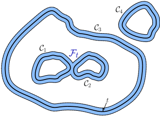
Figure 3. Sketch of a set $\Omega^{(0)}$ with boundary $\partial\Omega^{(0)}={\mathcal{C}}_{1}\cup$ ${\mathcal{C}}_{2}\cup{\mathcal{C}}_{3}$ $\cup{\mathcal{C}}_{4}$ and its $t$–neighborhood $\mathcal{N}_{t}(\partial\Omega^{(0)})$. The connected component ${\mathcal{F}}_{t}$ of $\mathcal{N}_{t}(\partial\Omega^{(0)})$ is generated by the loops ${\mathcal{C}}_{1}$ and ${\mathcal{C}}_{2}$.

Let $\ell_{t}:=d_{\partial G}^{-1}(t)\subset\mathbb{R}^{2}$ be the $t$-level set of $d_{\partial G}$. Let $\widetilde{\mathcal{N}_{t}}$ be the completion of $\mathcal{N}_{t}$ with respect to the intrinsic metric $\rho_{\mathcal{N}_{t}}$, where $\rho_{\mathcal{N}_{t}}(x,y)$ is defined as the infimum of the Euclidean length of curves joining $x$ and $y$ in $\mathcal{N}_{t}$, and let $\widetilde{\ell_{t}}:=\widetilde{\mathcal{N}_{t}}\backslash\mathcal{N}_{t}$. We note that $\widetilde{\mathcal{N}_{t}}$ admits a surjective $1$-Lipschitz map to the closure $\overline{\mathcal{N}}_{t}$ (w.r.t the standard metric) of $\mathcal{N}_{t}$, which induces a surjective 1-Lipschitz map $\widetilde{\ell_{t}}\rightarrow\ell_{t}\subset\mathbb{R}^{2}$; this implies $\mathcal{H}^{1}(\widetilde{\ell_{t}})\geq\mathcal{H}^{1}(\ell_{t})$. The inequality can be strict since tangentially aligned boundaries of different components are counted twice for $\tilde{\ell}_{t}$ (see Fig 3). By construction, $\tilde{\ell}_{t}$ consists of a collection of oriented, closed, piecewise $C^{2}$ curves with a finite number of vertex points ${\mathcal{V}}_{t}\subset\widetilde{\ell_{t}}$. We choose the orientation of each curve such that $\mathcal{N}_{t}$ lies to its left and write $\tau_{t}$ for the total rotation of $\widetilde{\ell_{t}}$. We also denote the rotation at the vortex points $x^{*}\in{\mathcal{V}}_{t}$ by $\tau_{x^{*}}\in[-\pi,0)$, noting that the case $\tau_{x^{*}}>0$ does not occur since such singularities are smoothed out (see Fig. 3).

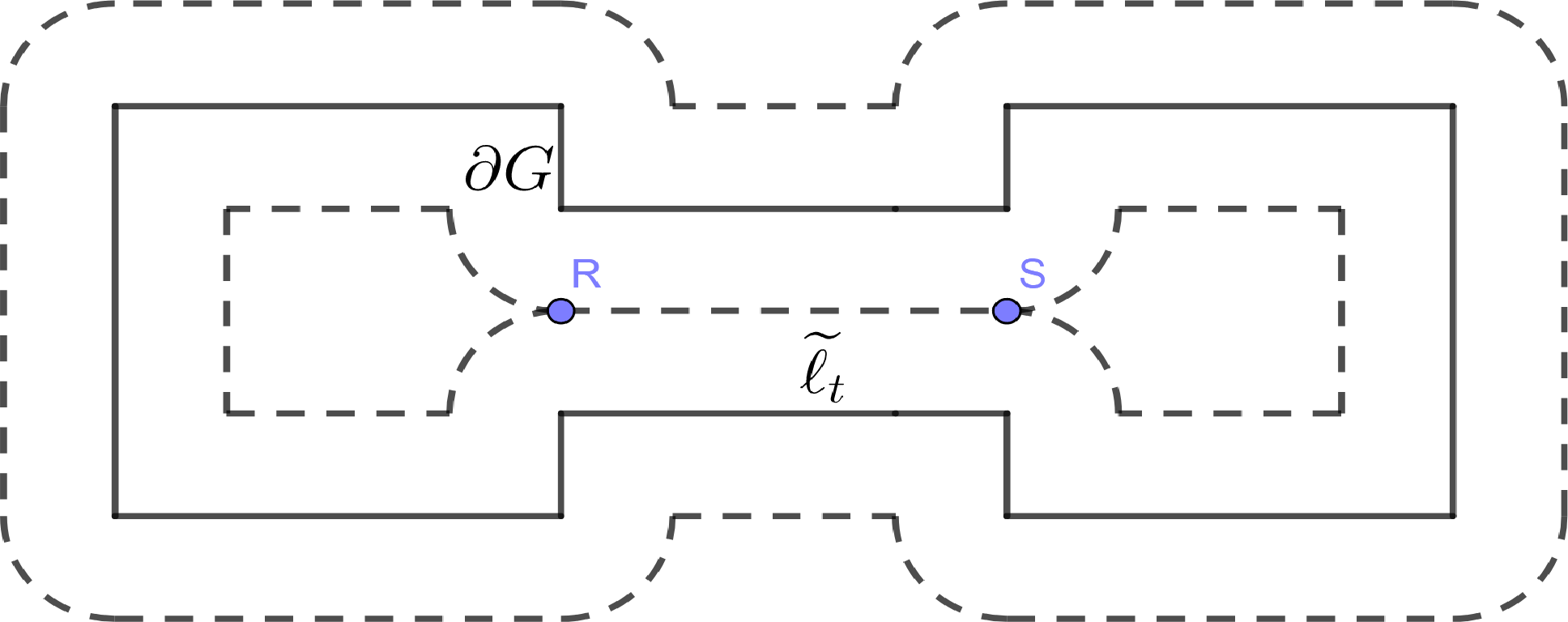
Figure 2. Level set associated to the boundary of a polygonal domain: The level set $\ell_{t}=d_{\partial G}^{-1}(t)$ is given by the dashed lines. For the curve $\tilde{\ell}_{t}$ coming from the metric completion, the line between $R$ and $S$ is counted twice.

We define $g(t):={\mathcal{H}}^{1}(\widetilde{\ell_{t}})$ for $t>0$ and $g(0):=\lim_{t\to 0}g(t)=2{\mathcal{H}}^{1}(\ell_{0})$. It is then enough to show that

$$g(t)\ \leq\ g(0)\qquad\qquad\text{ for $t\in\big{[}0,t_{0}\big{]}$}.$$ (37)

Proof of (37): We have $g\in C^{1}(\mathbb{R}\backslash\SS)$ for some finite set $\SS\subset[0,\infty)$ with

$$g^{\prime}(t)\ =\ \tau_{t}\ -\ \sum_{x^{*}\in{\mathcal{V}}_{t}}\Big{(}\tau_{x^{*}}-2\tan\frac{\tau_{x^{*}}}{2}\Big{)}\qquad\text{for $t\in[0,\infty)\backslash\SS$, }$$ (38)

and $g(t+0)\leq g(t-0)$ for any $t\in\SS$ [7, Lemma 3.2.3] (note that only the ”inner” level set $G\cap(\widetilde{\mathcal{N}_{t}}\backslash\mathcal{N}_{t})$ and with reverse orientation of the curves is considered in [7]). By the Gauss-Bonnet theorem, we have $\tau_{t}\ =\ 2\pi\chi(\mathcal{N}_{t})$ for $t>0$, which implies $\tau_{t}\ \leq\ 0$ for $t\in(0,t_{*}]$ by (36). We also note that $\varphi-2\tan\frac{\varphi}{2}\geq 0$ for $\varphi\in[-\pi,0]$. Hence, by integrating (38) over $(0,t)$, i.e.

$$g(t)\ \leq\ g(0)+\int_{0}^{t}\tau_{s}\ ds\ \leq\ g(0)\qquad\text{ for }t\in[0,t_{*}],$$ (39)

it follows that (37) holds for $t\in[0,t_{*}]$.

It remains to show (37) for $t\in(t_{*},t_{0}]$: Without loss of generality, we can assume that $t_{*}<t_{0}$. In this case, $g$ may have a downward–jump at $t_{*}$, i.e. $g(t_{*}+0)<g(t_{*}-0)$. Furthermore, for $t>t_{*}$ we have $\mathcal{N}_{t}$ $=$ $\mathcal{N}_{t}(\partial G)$ $=$ $\mathcal{N}_{t}(G)$, where $\mathcal{N}_{t}(G)$ is the $t$-neighborhood of $G$. We define $\widetilde{h_{t}}:=\widetilde{\mathcal{N}_{t}(G)}\backslash\mathcal{N}_{t}(G)$ for $t\geq 0$, where $\widetilde{\mathcal{N}_{t}(G)}$ is the completion of $\mathcal{N}_{t}(G)$ with respect to the intrinsic metric $\rho_{\mathcal{N}_{t}(G)}$. For $t\geq 0$, we define $f(t):={\mathcal{H}}^{1}(\widetilde{h_{t}})$ and $f(0):=\lim_{t\to 0}f(t)={\mathcal{H}}^{1}(\partial G)$. With the same arguments as before we then get

$$f(t)\ \leq\ f(0)+2\pi\int_{0}^{t}\chi(\mathcal{N}_{t}(G))\ ds\ \leq\ {\mathcal{H}}^{1}(\partial G)+2\pi t\qquad\text{ for }t\geq 0,$$ (40)

where we have used that $\chi(\mathcal{N}_{t}(G))\leq 1$ for all $t\geq 0$. By construction, for $t>t_{*}$, the inner level sets are empty and we thus have $g(t)=f(t)$. In particular, for $2\pi t\leq{\mathcal{H}}^{1}(\partial G)$ we have $g(t)\leq 2{\mathcal{H}}^{1}(\partial G)$. ∎

For not simply connected sets, the level set estimate in Lemma 2.1 does not hold in general: a simple counterexample is given by the annulus $B_{1}\backslash\overline{B_{\delta}}$ for $\delta\in(0,\frac{1}{4})$.

Generally, there is a decomposition $\Omega=\Omega^{(0)}\Delta\Omega^{(1)}$ such that $\Omega^{(0)}$ satisfies a level set estimate and such that the connected components of $\Omega^{(1)}$ have controlled size:

Lemma 2.2 (Global level set estimate).

Let $\Omega$ be a bounded open subset in $\mathbb{R}^{2}$ with piecewise $C^{2}$ boundary and let $0<\delta_{0}<\frac{1}{2\pi}\mathcal{H}^{1}(\partial\Omega)$. Then there exist two open subsets $\Omega^{(0)}$, $\Omega^{(1)}$ of the convex hull of $\Omega$ with $\Omega=\Omega^{(0)}\Delta\Omega^{(1)}$ and $\partial\Omega=\partial\Omega^{(0)}\cup\partial\Omega^{(1)}$such that the following holds:

1. The set $\Omega_{0}$ satisfies the level set estimate

   $${\mathcal{H}}^{1}(d_{\partial\Omega^{(0)}}^{-1}(t))\ \leq\ 2{\mathcal{H}}^{1}(\partial\Omega^{(0)})\qquad\qquad\text{for a.e. $t\in\big{[}0,\delta_{0}]$.}$$ (41)

2. For any connected component $G$ of $\Omega^{(1)}$, we have

   $${\mathcal{H}}^{1}(\partial G)\ \leq\ 2\pi\min\{\delta_{0},\operatorname*{dist}(\partial G,\partial\Omega^{(0)})\}.$$ (42)

Proof.

Construction: Since $\Omega$ is bounded with piecewise $C^{2}$ boundary, its boundary consists of finitely many simple closed curves ${\mathcal{C}}_{k}\subset\partial\Omega$, $k\in{\mathcal{I}}$. Furthermore, by using polygon approximation (similar as in Lemma 2.1) one may assume that each ${\mathcal{C}}_{k}$ is piecewise linear and the distance $d_{ij}:=\operatorname*{dist}({\mathcal{C}}_{i},{\mathcal{C}}_{j})$ between ${\mathcal{C}}_{i}$ and ${\mathcal{C}}_{j}$ are positive and pairwise different. By the Jordan-Schoenflies theorem, there is a unique decomposition

$$\Omega\ =\ \bigcup_{k\in{\mathcal{I}}_{+}}\bigg{(}G^{(k)}\backslash\bigcup_{\begin{subarray}{c}j\in{\mathcal{I}}_{-},G^{(j)}\subset G^{(k)}\end{subarray}}\overline{G^{(j)}}\bigg{)}$$ (43)

for some index set ${\mathcal{I}}_{+}$ and ${\mathcal{I}}_{-}$, where $G^{(k)}$, $k\in{\mathcal{I}}$, is the bounded simply connected domain with ${\mathcal{C}}_{k}=\partial G^{(k)}$. Roughly speaking, $\Omega$ is a union of finitely many connected components, where each component is a simply connected domain minus the closure of finitely many simply connected domains. We set ${\mathcal{I}}_{00}:=\{j\in{\mathcal{I}}:{\mathcal{H}}^{1}({\mathcal{C}}_{j})\geq 2\pi\delta_{0}\}$ and iteratively define

$${\mathcal{I}}_{0k}\ :=\ \Big{\{}\ell\in{\mathcal{I}}\ :\ {\mathcal{H}}^{1}({\mathcal{C}}_{\ell})\ \geq\ 2\pi\operatorname*{dist}\big{(}{\mathcal{C}}_{\ell},\bigcup\nolimits_{j\in\cup_{i=0}^{k-1}{\mathcal{I}}_{0i}}{\mathcal{C}}_{j}\big{)}\ \Big{\}}\qquad\text{for $k\geq 1$ .}$$ (44)

With ${\mathcal{I}}_{0}:=\bigcup_{i=0}^{\infty}{\mathcal{I}}_{0i}$, ${\mathcal{I}}_{1}:={\mathcal{I}}\backslash{\mathcal{I}}_{0}$ and ${\mathcal{I}}_{j}^{\pm}:={\mathcal{I}}_{j}\cap{\mathcal{I}}_{\pm}$ for $j=0,1$, we then define

$$\Omega^{(0)}\ :=\ \bigcup_{k\in{\mathcal{I}}_{0}^{+}}\bigg{(}G^{(k)}\backslash\bigcup_{\begin{subarray}{c}j\in{\mathcal{I}}_{0}^{-},G^{(j)}\subset G^{(k)}\end{subarray}}\overline{G^{(j)}}\bigg{)}\quad\text{and}\quad\Omega^{(1)}:=\Omega\Delta\Omega^{(0)}.$$ (45)

Note that if $k\in{\mathcal{I}}_{1}^{+}$, then by our selection procedure $\{j\in{\mathcal{I}}:G^{(j)}\subset G^{(k)}\}\subset{\mathcal{I}}_{1}$. In other words, if an outer loop ${\mathcal{C}}_{k}$ is not selected for $\Omega^{(0)}$, then the whole component $G^{(k)}$ is not contained in $\Omega^{(0)}$. Similarly, if $k\in{\mathcal{I}}_{1}^{-}$, then $\{j\in{\mathcal{I}}:G^{(j)}\subset G^{(k)}\}\subset{\mathcal{I}}_{1}$. Thus $\Omega^{(1)}$ is the union of $G^{(k)}$, where $k\in{\mathcal{I}}_{1}^{+}\cup{\mathcal{I}}_{1}^{-}$.

Conclusion of proof: By construction, the open sets $\Omega^{(0)}$, $\Omega^{(1)}$ are subsets of the convex hull of $\Omega$ and satisfy $\Omega=\Omega^{(0)}\Delta\Omega^{(1)}$ and $\partial\Omega=\partial\Omega^{(0)}\cup\partial\Omega^{(1)}$. Moreover, (42) holds since by construction for any $\ell\in{\mathcal{I}}_{1}$ we have ${\mathcal{H}}^{1}({\mathcal{C}}_{\ell})\leq 2\pi\delta_{0}$ and ${\mathcal{H}}^{1}({\mathcal{C}}_{\ell})\leq 2\pi\operatorname*{dist}({\mathcal{C}}_{\ell},\bigcup_{j\in{\mathcal{I}}_{0}}{\mathcal{C}}_{j})$. Hence, it remains to prove (i). In the sequel we write $\mathcal{N}_{t}(E):=\{x\in\mathbb{R}^{2}:\operatorname*{dist}(x,E)<t\}$ for the open $t$–neighborhood of $E$ for any set $E\subset\mathbb{R}^{2}$ and any $t>0$.

The number of connected components $N_{t}$ of the $t$-neighborhood of $\mathcal{N}_{t}(\partial\Omega^{(0)})$ of $\partial\Omega^{(0)}$ is nonincreasing in $t$ and piecewise constant, except at a finite number of merging times, when components merge. We consider any interval $I=(t_{0},t_{1}]$ such that $N_{t}$ is constant in $I$ and $t_{0}<t_{1}$ are either merging times or $t_{0},t_{1}\in\{0,\delta_{0}\}$. Then it is enough to show (41) for every single connected component of $\mathcal{N}_{t}(\partial\Omega^{(0)})$, $t\in I$. Within this time interval, we consider any connected component ${\mathcal{F}}_{t_{1}}\subset\mathcal{N}_{t_{1}}(\partial\Omega^{(0)})$. Upon relabelling we can assume that the loops contained in ${\mathcal{F}}_{t_{1}}$ are given by ${\mathcal{C}}_{i}=\partial G^{(i)}$, $1\leq i\leq N$ for some $N\in\mathbb{N}$. We write

$${\mathcal{F}}_{t}\ :=\ \mathcal{N}_{t}\big{(}\bigcup_{i=1}^{N}{\mathcal{C}}_{i}\big{)}\ \subset\ \mathcal{N}_{t}(\partial\Omega^{(0)})\qquad\text{for $t>0$}$$ (46)

for the $t$-neighborhood associated to the loops $\{{\mathcal{C}}_{i}\}_{i=1}^{N}$. Therefore, it suffices to show that

$${\mathcal{H}}^{1}(\partial{\mathcal{F}}_{t})\ \leq\ 2\sum_{i=1}^{N}c_{i},\qquad\text{for $t\in I=(t_{0},t_{1}]$ where $c_{i}:={\mathcal{H}}^{1}({\mathcal{C}}_{i})$.}$$ (47)

By construction ${\mathcal{F}}_{t}$ is connected for all $t\in I$ (as ${\mathcal{F}}_{t_{1}}$ is connected and there is no merging time in $I$) and thus the Euler characteristics satisfies $\chi({\mathcal{F}}_{t})\leq 1$ for $t\in I$.

Proof of (47): By [7, Lemma 3.2.3], ${\mathcal{H}}^{1}(\partial{\mathcal{F}}_{t})$ can only have a downward jump discontinuity. Hence, by finite induction we can assume that (47) holds at time $t_{0}+0$, i.e $\lim_{t\searrow t_{0}}{\mathcal{H}}^{1}(\partial{\mathcal{F}}_{t})\ \leq\ 2\sum_{i=1}^{N}c_{i}$. We choose $t_{*}\in[t_{0},t_{1}]$ maximal such that $\chi({\mathcal{F}}_{t})\leq 0$ in $(t_{0},t_{*}]$. If $t_{*}$ does not exist, then we set $t_{*}=t_{0}$. If $t_{*}>t_{0}$ then the same argument as for (39) shows that ${\mathcal{H}}^{1}(\partial{\mathcal{F}}_{t})$ is nonincreasing for $t\in(t_{0},t_{*}]$. Together with the induction hypothesis this shows that (47) holds for $t\in(t_{0},t_{*}]$.

It remains to show (47) for $t\in(t_{*},t_{1}]$: Without loss of generality, we can assume that $t_{*}<t_{1}$. By definition of $t_{*}$ we have $\lim_{t\searrow t_{*}}\chi({\mathcal{F}}_{t})=1$ (note that $\chi({\mathcal{F}}_{t})\leq 1$ for $t\in I$ since ${\mathcal{F}}_{t}$ is connected in $I$). Since ${\mathcal{F}}_{t}$ is connected, this implies that ${\mathcal{F}}_{t}$ is simply connected for $t=t_{*}+0$. It follows that $G^{(i)}\subset{\mathcal{F}}_{t}$ for $t>t_{*}$ and for all $1\leq i\leq N$. In particular, with the notation

$${\mathcal{G}}_{t}\ :=\ \mathcal{N}_{t}\big{(}\bigcup_{i=1}^{N}G^{(i)}\big{)}\qquad\text{for $t>0$}$$ (48)

we have ${\mathcal{F}}_{t}={\mathcal{G}}_{t}$ for $t>t_{*}$. It then is enough to show

$${\mathcal{H}}^{1}(\partial{\mathcal{G}}_{t})\ \leq\ 2\sum_{i=1}^{N}c_{i}\qquad\text{for all $t\in(t_{*},t_{1}].$}$$ (49)

In fact, we will show that (49) holds for all $t\in[0,t_{1})$.

We recall that by construction ${\mathcal{F}}_{0}$ consists of $N$ connected components and ${\mathcal{F}}_{t}$ is connected for all $t\in I$. Furthermore, since the set of merging times of the connected components of ${\mathcal{F}}_{t}$ for $t\in(0,t_{1}]$ is a subset of $\{\frac{1}{2}d_{ij}\}$ with $d_{ij}$ pairwise different by our assumption at the beginning of the proof, hence there are $N-1$ merging times $0<s_{1}<s_{2}<\ldots<s_{N-1}\leq t_{1}$ for connected components in ${\mathcal{F}}_{t}$. Moreover, the number of connected components of ${\mathcal{F}}_{t}$ decreases by precisely $1$ at each merging time. Thus in the time interval $(s_{i-1},s_{i}]$ we have $N_{i}:=N-i+1$ connected components for $1\leq i\leq N$, where we have set $s_{0}:=0$ and $s_{N}:=t_{1}$.

Since the length of the outer boundary ${\mathcal{H}}^{1}(\partial{\mathcal{G}}_{t})$ grows at a rate of at most $2\pi$ for each single component of ${\mathcal{G}}_{t}$ (cf. (40)), and moreover, the number of components of ${\mathcal{G}}_{t}$ is no larger than the number of components of ${\mathcal{F}}_{t}$ for each $t\in(0,t_{1}]$, integrating over $(0,t)$ yields

$${\mathcal{H}}^{1}(\partial{\mathcal{G}}_{t})\ \leq\ \sum_{i=1}^{N}c_{i}+2\pi\sum_{i=1}^{N}N_{i}(s_{i}-s_{i-1})\ =\ \sum_{i=1}^{N}c_{i}+2\pi\sum_{i=1}^{N}s_{i}.$$ (50)

We want to show that $2\pi\sum_{i=1}^{N}s_{i}\leq\sum_{i=1}^{N}c_{i}$. Without loss of generality, we assume $c_{1}\geq\ldots\geq c_{N}$. Let $\{{\mathcal{F}}_{s_{i}}^{(j)},1\leq j\leq N_{i}\}$ be the set of connected components included in ${\mathcal{F}}_{t}$ for $t\in(s_{i-1},s_{i}]$, and let ${\mathcal{J}}_{s_{i}}^{(j)}$ be the corresponding index set of the loops ${\mathcal{C}}_{\ell}$, $\ell\in{\mathcal{J}}_{s_{i}}^{(j)}$, included in ${\mathcal{F}}_{s_{i}}^{(j)}$, i.e. ${\mathcal{F}}_{s_{i}}^{(j)}=\mathcal{N}_{t}(\bigcup_{\ell\in{\mathcal{J}}_{s_{i}}^{(j)}}{\mathcal{C}}_{\ell})$ for $t\in(s_{i-1},s_{i}]$. From our construction (44) and since $s_{i}\leq\delta_{0}$, we have

$$2\pi s_{i}\ \stackrel{{\scriptstyle\eqref{eq-I00}}}{{\leq}}\ \min_{1\leq j\leq N_{i}}\ \max_{k\in{\mathcal{J}}_{s_{i}}^{(j)}}\ c_{k}\ \ \leq\ c_{1+(N_{i}-1)}\ =\ c_{N-i+1}.$$ (51)

Inserting (51) into (50), we obtain (49) for $t\in(0,t_{1}]$. ∎

For a sufficiently regular set $\Omega\subset\mathbb{R}^{2}$ and for some $\widehat{x}\in\mathbb{R}^{2}$ and $\rho>0$, we next derive a local level set estimate for $\partial\Omega\cap B_{\rho}(\widehat{x})$.

Theorem 2.3 (Local level set estimate).

Let $\Omega\Subset\mathbb{R}^{2}$ be bounded and open with $\partial\Omega\in C^{2}$. For $\hat{x}\in\mathbb{R}^{2}$, $\rho>0$ let $B_{\rho}:=B_{\rho}(\hat{x})$ and suppose that $\Omega\cap B_{\rho}\neq\emptyset$. Let $0<2\pi\delta_{0}\leq\min\{\frac{\rho}{8},{\mathcal{H}}^{1}(\partial\Omega\cap B_{\rho})\}$. Then there exist two subsets $\Omega_{\rho}^{(0)},\Omega_{\rho}^{(1)}\subset B_{\rho}$ with

$$\Omega\cap B_{\rho-2\delta_{0}}\ =\ (\Omega_{\rho}^{(0)}\Delta\Omega_{\rho}^{(1)})\cap B_{\rho-2\delta_{0}}$$ (52)

such that with $\gamma_{\rho}:=\partial\Omega^{(0)}_{\rho}\cap B_{\rho}$ the following holds:

1. The length of the boundaries is estimated by

   $$\max\{\mathcal{H}^{1}(\gamma_{\rho}),{\mathcal{H}}^{1}(\partial\Omega^{(1)}_{\rho}\cap B_{\rho})\}\ \leq\ {\mathcal{H}}^{1}(\partial\Omega\cap B_{\rho}).$$ (53)

2. We have the level set estimate

   $${\mathcal{H}}^{1}(d_{\gamma_{\rho}}^{-1}(t)\cap B_{\rho-4\delta_{0}})\ \leq\ 2{\mathcal{H}}^{1}(\gamma_{\rho})\quad\qquad\text{for a.e. $t\in(0,\delta_{0})$.}$$ (54)

3. Any connected component $G$ of $\Omega_{\rho}^{(1)}\cap B_{\rho-2\delta_{0}}$ satisfies

   $${\mathcal{H}}^{1}(\partial G)\ \leq\ 2\pi\min\{\delta_{0},\operatorname*{dist}(\partial G,\gamma_{\rho})\}.$$ (55)

Proof.

Let $\Omega_{\rho}:=\Omega\cap B_{\rho}$ and $S_{2\delta_{0}}:=B_{\rho}\backslash\overline{B_{\rho-2\delta_{0}}}$. We first construct a new set $\tilde{\Omega}_{\rho}$ such that

$$\tilde{\Omega}_{\rho}\cap B_{\rho-2\delta_{0}}\ =\ \Omega_{\rho}\cap B_{\rho-2\delta_{0}},$$ (56)

$$\mathcal{H}^{1}(\partial\tilde{\Omega}_{\rho}\cap B_{\rho})\ \leq\ \mathcal{H}^{1}(\partial\Omega\cap B_{\rho}).$$ (57)

Furthermore, every connected component $U$ of $\tilde{\Omega}_{\rho}\cap S_{2\delta_{0}}$ and every connected component of $(\tilde{\Omega}_{\rho}^{c})^{o}\cap S_{2\delta_{0}}$ is a sufficiently wide annulus sector of the form

$$U\ =\ \{\hat{x}+re^{i\varphi}:r\in(\rho-2\delta_{0},\rho),\varphi\in(\theta,\theta+\Delta\theta)\text{ or }[0,2\pi)\}\ \text{with $\rho\Delta\theta>4\delta_{0}$}$$ (58)

for some $\theta,\Delta\theta\in[0,2\pi)$, see Fig. 4 for an illustration of the set and the construction. We then apply Lemma 2.2 to the modified set $\tilde{\Omega}_{\rho}$.

Construction of $\tilde{\Omega}_{\rho}$: To construct $\tilde{\Omega}_{\rho}$, we modify iteratively $\Omega_{\rho}$ as follows:

• We remove any connected component $U$ of $\Omega_{\rho}\cap S_{2\delta_{0}}$ such that

  $${\mathcal{H}}^{1}(\partial U\cap\partial B_{\rho})\ =\ 0\qquad\text{or}\qquad{\mathcal{H}}^{1}(\partial U\cap\partial B_{\rho-2\delta_{0}})\ \leq\ 4\delta_{0}.$$ (59)

• We fill in the hole related to any connected component $V$ of $(\Omega_{\rho}^{c})^{o}\cap S_{2\delta_{0}}$ such that

  $${\mathcal{H}}^{1}(\partial V\cap\partial B_{\rho})\ =\ 0\qquad\text{or}\qquad{\mathcal{H}}^{1}(\partial V\cap\partial B_{\rho-2\delta_{0}})\ \leq\ 4\delta_{0}.$$ (60)

We note that the above modifications might create a new boundary portion along $\partial B_{\rho-2\delta_{0}}$. However, the total length of the boundary is not increased: If we e.g. remove a connected component $U$, then we might create a new boundary at $\partial B_{\rho-2\delta_{0}}\cap\partial U$ for the modified set. However, if ${\mathcal{H}}^{1}(\partial U\cap\partial B_{\rho})=0$, then removing $U$ does not increase the total length of the boundary (since the inner set $B_{\rho-2\delta_{0}}$ is convex). If ${\mathcal{H}}^{1}(\partial U\cap\partial B_{\rho-2\delta_{0}})\neq 0$ and ${\mathcal{H}}^{1}(\partial U\cap\partial B_{\rho})\leq 4\delta_{0}$ then again the total length of the boundary does not increase (since $\partial B_{\rho-2\delta_{0}}$ and $\partial B_{\rho}$ have distance $2\delta_{0}$). We note that the final set after application of the above algorithm is not unique (and depends on the order of steps taken). Our argument, however, works independently on the specific choice final set.

For any remaining connected component $U$ of $\Omega_{\rho}\cap S_{2\delta_{0}}$, one has ${\mathcal{H}}^{1}(\partial U\cap\partial B_{\rho})>0$ and ${\mathcal{H}}^{1}(\partial U\cap\partial B_{\rho-2\delta_{0}})>4\delta_{0}$, and moreover $\partial U\cap\partial B_{\rho-2\delta_{0}}=\{\widehat{x}+(\rho-2\delta_{0})e^{i\varphi}:\varphi\in[\theta,\theta+\Delta\theta])\}$ for some $\theta,\Delta\theta\in[0,2\pi)$. Then for any such connected component

• we replace $U$ by the annulus sector of the form (58) with $\theta,\Delta\theta$ as above.

By construction, also this modification does not increase the total length of the relative boundary in $B_{\rho}$. After applying these modifications, we hence obtain a set $\tilde{\Omega}_{\rho}$ which satisfies the conditions (56), (57) and (58).

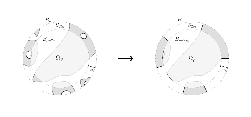
Figure 4. Illustration for the construction of $\tilde{\Omega}_{\rho}$.

Conclusion of proof: Let $\Omega_{\rho}^{(0)}$ and $\Omega_{\rho}^{(1)}$ be the sets constructed in Lemma 2.2 (with $\Omega$ replaced by $\tilde{\Omega}_{\rho}$). In view of (56), assertions (52) and (55) follow directly from Lemma 2.2. Assertion (53) follows from (57) and since by Lemma 2.2 we have $\partial\Omega_{\rho}^{(i)}\cap B_{\rho}\subset\partial\tilde{\Omega}_{\rho}\cap B_{\rho}$ for $i=0,1$.

In order to show (54), we note that by Lemma 2.2(i)

$${\mathcal{H}}^{1}(d_{\partial\Omega_{\rho}^{(0)}}^{-1}(t))\ \leq\ 2{\mathcal{H}}^{1}(\partial\Omega_{\rho}^{(0)})\qquad\qquad\text{for a.e. $t\in(0,\delta_{0})$}.$$ (61)

Since ${\mathcal{H}}^{1}(\partial\Omega_{\rho}^{(0)})={\mathcal{H}}^{1}(\gamma_{\rho})+{\mathcal{H}}^{1}(\partial\Omega_{\rho}^{(0)}\cap\partial B_{\rho})$ and since $d_{\partial\Omega_{\rho}^{(0)}}^{-1}(t)\cap\overline{B_{\rho-4\delta_{0}}}\supseteq d_{\gamma_{\rho}}^{-1}(t)\cap B_{\rho-4\delta_{0}}$, then from (61) one has

$${\mathcal{H}}^{1}(d_{\gamma_{\rho}}^{-1}(t)\cap B_{\rho-4\delta_{0}})+{\mathcal{H}}^{1}(d_{\partial\Omega_{\rho}^{(0)}}^{-1}(t)\cap(B_{\rho+\delta_{0}}\backslash B_{\rho-4\delta_{0}}))\leq 2{\mathcal{H}}^{1}(\gamma_{\rho})+2{\mathcal{H}}^{1}(\partial\Omega_{\rho}^{(0)}\cap\partial B_{\rho}).$$ (62)

Thus (54) follows if we can show that

$$2{\mathcal{H}}^{1}(\partial\Omega_{\rho}^{(0)}\cap\partial B_{\rho})\ \leq\ {\mathcal{H}}^{1}(d_{\partial\Omega_{\rho}^{(0)}}^{-1}(t)\cap(B_{\rho+\delta_{0}}\backslash B_{\rho-4\delta_{0}}))\quad\text{ for a.e. }t\in(0,\delta_{0}).$$ (63)

We will prove (63) by making use of the simple geometry of $\Omega^{(0)}_{\rho}$ in $S_{2\delta_{0}}$: Indeed, by construction $\Omega^{(0)}_{\rho}\cap S_{2\delta_{0}}$ and $(\Omega^{(0)}_{\rho})^{c}\cap S_{2\delta_{0}}$ consist of finitely many disjoint annulus sectors of the form (58). Thus in view of the simple geometry for any connected component $U$ of $\Omega_{\rho}^{(0)}\cap S_{2\delta_{0}}$ we have

$$2{\mathcal{H}}^{1}(\partial U\cap\partial B_{\rho})\ \leq\ {\mathcal{H}}^{1}(d_{\partial U}^{-1}(t)\cap(B_{\rho+\delta_{0}}\backslash B_{\rho-\delta_{0}}))\quad\text{ for }t\in(0,\delta_{0}),$$ (64)

We note that $\partial\Omega_{\rho}^{(0)}\cap\partial B_{\rho}$ is the disjoint union of the sets $\partial U\cap\partial B_{\rho}$ for connected components $U$ of $\Omega_{\rho}^{(0)}\cap S_{2\delta_{0}}$ and — by the geometry of $\Omega_{\rho}^{(0)}$ — the set $d_{\partial\Omega_{\rho}^{(0)}}^{-1}(t)\cap(B_{\rho+\delta_{0}}\backslash B_{\rho-4\delta_{0}})$ contains the union of the sets $d_{\partial U}^{-1}(t)\cap(B_{\rho+\delta_{0}}\setminus B_{\rho-\delta_{0}})$. Furthermore, by construction the sets $d_{\partial U}^{-1}(t)\cap(B_{\rho+\delta_{0}}\setminus B_{\rho-\delta_{0}})$ and $d_{\partial V}^{-1}(t)\cap(B_{\rho+\delta_{0}}\setminus B_{\rho-\delta_{0}})$ are disjoint for any two different connected components $U,V$ of $\Omega_{\rho}^{(0)}\cap S_{2\delta_{0}}$. The estimate (63) then follows summing up the estimates (64) for each connected component $U$.

∎

2.2. Construction of test function

For the proof of the liminf inequality (8) in Theorem 1.1, we need to show that for any sequence $m_{\epsilon}\in{\mathcal{A}}$ with $m_{\epsilon}\to m\in{\mathcal{A}}_{0}$ in $L^{1}$ we have $\liminf_{\epsilon>0}E_{\epsilon}[m_{\epsilon}]\ \geq\ E_{0}[m]$. For the proof, we may assume that the functions are smooth, i.e. we consider sequences $m_{\epsilon}$ which satisfy

$$\begin{aligned} &m_{\epsilon}\to m\text{ in $L^{1}$ as $\epsilon\to 0$}\\ &\qquad\text{ where }m_{\epsilon}=(u_{\epsilon},v_{\epsilon})\in{\mathcal{A}}\cap C^{\infty}(Q_{\ell};\mathbb{S}^{1})\text{ and where }m=(u,0)\in{\mathcal{A}}_{0}.\end{aligned}$$ (65)

Indeed, for a general sequence $m_{\epsilon}\in{\mathcal{A}}$ one can consider functions $m_{\epsilon,k}\in{\mathcal{A}}\cap C^{\infty}(Q_{\ell};\mathbb{S}^{1})$ with $m_{\epsilon,k}\to m_{\epsilon}$ in $H^{1}$ for $k\to\infty$. In particular, since the energy is continuous with respect to the $H^{1}$–norm, we also have $E_{\epsilon}[m_{\epsilon,k}]\to E_{\epsilon}[m_{\epsilon}]$ as $k\to\infty$. For the proof of the liminf inequality, it is then enough to consider smooth $m_{\epsilon}$ by taking a diagonal sequence. Throughout the section, we will also use the notation

$$\Omega_{0}\ :=\ \{x\in Q_{\ell}\ :\ u(x)\ =\ 1\},$$ (66)

$$\SS_{m}\ :=\ \partial^{*}\Omega_{0}\text{ with measure theoretic outer normal $n$.}$$ (67)

Since we often need logarithmic lengh scales, for notational convenience, we write

$$\delta_{\epsilon}\ :=\ \frac{1}{|\ln\epsilon|^{\frac{1}{4}}}\qquad$$ (68)

throughout this work. For the proof of the liminf inequality we use the strategy explained in Section 1.1. For this, we first give the construction of the test functions $\Phi_{\epsilon,\rho}$ (cf. (25)), associated with the sequence $m_{\epsilon}$ and localized on the ball $B_{\rho}:=B_{\rho}(\widehat{x})$ for some fixed $\rho\in(0,1)$. We start with the construction of the separating curves $\gamma_{\epsilon,\rho}:=\gamma_{\epsilon,B_{\rho}(\widehat{x})}$ with $\widehat{x}\in\SS_{m}$ (cf. Lemma 2.5). For that, we first choose suitable superlevel sets, whose boundaries converge weakly to the jump set of the limit $m$ in $B_{\rho}$ and satisfy a uniform upper bound on the lengths of their boundary:

Lemma 2.4 (Choice of superlevel sets).

Consider a sequence $m_{\epsilon}\to m$ which satisfies (65) for some sequence $\epsilon\to 0$ and let $\Omega_{0}$, $\SS_{m}$, $n$ be given by (66). Let $\widehat{x}\in\SS_{m}$ and $\rho\in(0,1)$. Then there is a subsequence $\epsilon_{j}\to 0$ and a sequence $t_{j}\in(-1,1)$ with

$$|t_{j}|\ \leq\ 1-\delta_{\epsilon}\qquad\qquad\forall j\in\mathbb{N}$$ (69)

($\delta_{\epsilon}$ is given in (68)) such that the following holds: The superlevel sets

$$\Omega_{\epsilon_{j}}\ :=\ \{x\in Q_{\ell}:u_{\epsilon_{j}}>t_{j}\}$$ (70)

with outer normal $n_{\epsilon_{j}}$ satisfy $\partial\Omega_{\epsilon_{j}}\in C^{\infty}$. Furthermore, with $B_{\rho}:=B_{\rho}(\widehat{x})$ we have

1. $\chi_{\Omega_{\epsilon_{j}}}\to\chi_{\Omega_{0}}\text{ in }L^{1}(B_{\rho})$.

2. $D\chi_{\Omega_{\epsilon_{j}}}$ $\stackrel{{\scriptstyle*}}{{\rightharpoonup}}$ $D\chi_{\Omega_{0}}$ weakly^∗ in $B_{\rho}$.In particular,

   $$\|D\chi_{\Omega_{0}}\|(B_{\rho})\ \leq\ \liminf_{j\to\infty}\|D\chi_{\Omega_{\epsilon_{j}}}\|(B_{\rho})\ \leq\ \frac{K}{2}.$$ (71)

3. We have (cf. (21))

   $$\limsup_{j\to\infty}\frac{\|D\chi_{\Omega_{\epsilon_{j}}}\|(B_{\rho})}{\|D\chi_{\Omega_{0}}\|(B_{\rho})}\ \leq\ \alpha\ :=\ \liminf_{\epsilon\to 0}\frac{\|Du_{\epsilon}\|(B_{\rho})}{\|Du\|(B_{\rho})}.$$ (72)

Proof.

For $t\in(-1,1)$ and $\epsilon\geq 0$, we write $\Omega^{\epsilon}_{t}:=\{x\in Q_{\ell}:u_{\epsilon}>t\}$. We choose a subsequence $\epsilon_{j}\to 0$ such that $\lim_{j\to\infty}\|Du_{\epsilon_{j}}\|(B_{\rho})\rightarrow\alpha\|Du\|(B_{\rho})$, where $\alpha$ is given in (iii). Since $u_{\epsilon_{j}}\to u_{0}$ in $L^{1}(B_{\rho})$, by taking a further subsequence (not relabeled), we have $\chi_{\Omega^{\epsilon_{j}}_{t}}\to\chi_{\Omega^{0}_{t}}$ in $L^{1}(B_{\rho})$ for a.e. $t\in(-1,1)$, where $\Omega^{0}_{t}=\Omega_{0}$ for $t\in(-1,1)$. Since $\chi_{\Omega^{0}_{t}}=\chi_{\Omega_{0}}$ is independent of $t$ and $t\mapsto\chi_{\Omega^{\epsilon}_{t}}$ is monotonically decreasing, the convergence holds for any superlevel set,

$$\chi_{\Omega^{\epsilon_{j}}_{t}}\ \to\ \chi_{\Omega_{0}}\qquad\text{ in $L^{1}(B_{\rho})$ for any $t\in(-1,1)$}.$$ (73)

Let $\mathcal{S}_{j}\subset(-1,1)$ denote the set of singular values $t$ such that $\partial\Omega_{t}^{\epsilon_{j}}\cap B_{\rho}$ is not smooth for $t\in\SS_{j}$. Then $\mathcal{S}:=\bigcup_{j}\mathcal{S}_{j}$ has Lebesgue measure zero by Sard’s theorem. We aim to find a subsequence $(\epsilon_{\ell})_{\ell\in\mathbb{N}}$ of $\epsilon_{j}$ and a sequence $(t_{\ell})_{\ell\in\mathbb{N}}$ such that the assertions are satisfied. We claim that for any $\ell\in\mathbb{N}$ there exists $t_{\ell}\in(-1,1)\backslash\SS$ and a subsequence $(\epsilon_{j_{k}(\ell)})_{k\in\mathbb{N}}$ of $(\epsilon_{j})$ such that

$$\|D\chi_{\Omega^{\epsilon_{j_{k}(\ell)}}_{t_{\ell}}}\|(B_{\rho})\ \leq\ \alpha\|D\chi_{\Omega_{0}}\|(B_{\rho})+\frac{1}{\ell}\qquad\text{for all $k\in\mathbb{N}$.}$$ (74)

Indeed, if not, then $\|D\chi_{\Omega^{\epsilon_{j}}_{t}}\|(B_{\rho})>\alpha\|D\chi_{\Omega_{0}}\|(B_{\rho})+\frac{1}{\ell}$ for any $t\in(-1,1)\backslash\SS$ and for any $j\geq j_{0}(t)$ sufficiently large. By the coarea formula, we have

$$\|Du_{\epsilon_{j}}\|(B_{\rho})\ =\ \int_{-1}^{1}\|D\chi_{\Omega^{\epsilon_{j}}_{t}}\|(B_{\rho})\ dt.$$ (75)

Taking the limit in (75) and using (21) and (74) then implies $\alpha\|D\chi_{\Omega_{0}}\|(B_{\rho})$ $>$ $\alpha\|D\chi_{\Omega_{0}}\|(B_{\rho})+\frac{1}{\ell}$, which is a contradiction and hence yields (74).

For each fixed $\ell\in\mathbb{N}$, there is $k_{\ell}\in\mathbb{N}$ large such that $|t_{\ell}|<1-\delta_{\epsilon_{j_{k}(\ell)}}$ for all $k\geq k_{\ell}$. In view of (73), by making $k_{\ell}$ possibly larger we have $\|\chi_{\Omega^{\epsilon_{j_{k_{\ell}}(\ell)}}_{t_{\ell}}}-\chi_{\Omega_{0}}\|_{L^{1}(B_{\rho})}\leq\frac{1}{\ell}$. For the diagonal sequence $\epsilon_{\ell}:=\epsilon_{j_{k_{\ell}(\ell)}}$, we then have $|t_{\ell}|<1-\delta_{\epsilon_{\ell}}$, $\Omega_{\epsilon_{\ell}}$ has a smooth boundary and (i) holds. In view of (74), (iii) holds.

It remains to show (ii): In view of (i), we get

$$\int_{\Omega^{\epsilon_{\ell}}_{t_{\ell}}}\operatorname*{\ \nabla\-\cdot\-}\zeta\ dx\ \to\ \int_{\Omega_{0}}\operatorname*{\ \nabla\-\cdot\-}\zeta\ dx\qquad\qquad\text{for any $\zeta\in C^{1}_{c}(B_{\rho})$}.$$ (76)

From (iii), it follows that the sets $\Omega_{\epsilon_{\ell}}:=\Omega^{\epsilon_{\ell}}_{t_{\ell}}$ have uniformly bounded perimeter. Together with (76), this implies the weak convergence $D\chi_{\Omega_{\epsilon_{\ell}}}\stackrel{{\scriptstyle*}}{{\rightharpoonup}}D\chi_{\Omega_{0}}$. The second claim in (ii) follows from the lower semi-continuity of the total variation measure. ∎

The sets $\partial\Omega_{\epsilon_{j}}\cap B_{\rho}$, where $\Omega_{\epsilon_{j}}$ are the superlevel sets constructed in Lemma 2.4, cannot be directly used for the definition of the separating curves as described in Section 1.1, as the capacity of $\partial\Omega_{\epsilon_{j}}\cap B_{\rho}$ might be too large. However, using Theorem 2.3 in Section 2.1, in the next lemma we construct a slightly modified set $\Omega_{\epsilon_{j},\rho}^{(0)}\subset B_{\rho}$ which approximates $\Omega_{\epsilon_{j}}\cap B_{\rho}$ and such that $\gamma_{\epsilon_{j},\rho}:=\partial\Omega_{\epsilon_{j},\rho}^{(0)}\cap B_{\rho}$ satisfies the desired properties of the separating curves in Section 1.1:

Lemma 2.5 (Separating curves).

Consider a sequence $m_{\epsilon}\to m$ with $\epsilon\to 0$ which satisfies (65) and let $\Omega_{0}$, $\SS_{m}$, $n$ be given by (66). Then for any $\widehat{x}\in\SS_{m}$ there is $\hat{\rho}>0$ such that for any $\rho\in(0,\hat{\rho})$ the following holds: Let $\epsilon_{j}\to 0$ and $t_{j}\in(-1,1)$ be the sequences constructed in Lemma 2.4 and let $\Omega_{\epsilon_{j}}$ be defined by (70). Then there exist sets $\Omega_{\epsilon_{j},\rho}^{(0)},\Omega_{\epsilon_{j},\rho}^{(1)}\subset B_{\rho}(\widehat{x})=:B_{\rho}$ such that the following holds:

1. $\chi_{\Omega_{\epsilon_{j},\rho}^{(0)}}\to\chi_{\Omega_{0}}\text{ in }L^{1}(B_{\rho})$ as $j\to\infty$.

2. Let $\gamma_{\epsilon_{j},\rho}:=\partial\Omega_{\epsilon_{j},\rho}^{(0)}\cap B_{\rho}$ and let $n_{\epsilon_{j},\rho}$ be the outer normal of $\gamma_{\epsilon_{j},\rho}$ w.r.t. $\Omega_{\epsilon_{j},\rho}^{(0)}$. Then we have $n_{\epsilon_{j},\rho}{\mathcal{H}}^{1}\llcorner\gamma_{\epsilon_{j},\rho}\ \stackrel{{\scriptstyle*}}{{\rightharpoonup}}\ n{\mathcal{H}}^{1}\llcorner\SS_{m}$ in $B_{\rho}$. In particular

   $${\mathcal{H}}^{1}(\SS_{m}\cap B_{\rho})\ \leq\ \liminf_{j\to\infty}{\mathcal{H}}^{1}(\gamma_{\epsilon_{j},\rho}).$$ (77)

3. ${\mathcal{H}}^{1}(\gamma_{\epsilon_{j},\rho})\leq{\mathcal{H}}^{1}(\partial\Omega_{\epsilon_{j}}\cap B_{\rho})\leq K$.

4. We have

   $$\limsup_{{\epsilon_{j}}\to 0}\frac{{\mathcal{H}}^{1}(\gamma_{{\epsilon_{j}},\rho})}{{\mathcal{H}}^{1}(\SS_{m}\cap B_{\rho})}\ \leq\ \alpha\ :=\ \liminf_{\epsilon\to 0}\frac{\|Du_{\epsilon}\|(B_{\rho})}{\|Du\|(B_{\rho})}.$$ (78)

5. We have the level set estimate

   $$\qquad\qquad{\mathcal{H}}^{1}(d^{-1}_{\gamma_{{\epsilon_{j}},\rho}}(t)\cap B_{\rho-8\delta_{\epsilon_{j}}})\ \leq\ 2{\mathcal{H}}^{1}(\gamma_{{\epsilon_{j}},\rho})\quad\forall t\in(0,2\delta_{\epsilon_{j}}).$$ (79)

6. $|\Omega_{{\epsilon_{j}},\rho}^{(1)}|\ \leq\ C(K+1)\delta_{\epsilon_{j}}\ \to 0$    as $j\to\infty$.

7. ${\mathcal{H}}^{1}(\partial\Omega_{{\epsilon_{j}},\rho}^{(1)}\cap B_{\rho-4\delta_{\epsilon_{j}}})\ \leq\ {\mathcal{H}}^{1}(\partial\Omega_{\epsilon_{j}}\cap B_{\rho})\ \leq\ K$.

8. The connected components $G_{{\epsilon_{j}},\rho}^{(k)}$ of $\Omega_{{\epsilon_{j}},\rho}^{(1)}\cap B_{\rho-4\delta_{\epsilon_{j}}}$ satisfy

   $$\frac{1}{2\pi}{\mathcal{H}}^{1}(\partial G_{{\epsilon_{j}},\rho}^{(k)})\ \leq\ \min\{2\delta_{\epsilon_{j}},\operatorname*{dist}(\partial G_{{\epsilon_{j}},\rho}^{(k)},\gamma_{{\epsilon_{j}},\rho})\}.$$ (80)

9. We have

   $$1+u_{{\epsilon_{j}}}\ \geq\ \delta_{\epsilon_{j}} B_{\rho-4\delta_{\epsilon_{j}}}\cap\Omega_{{\epsilon_{j}},\rho}^{(0)}\backslash\Omega_{{\epsilon_{j}},\rho}^{(1)}$$ in , (81)

   $$1-u_{{\epsilon_{j}}}\ \geq\ \delta_{\epsilon_{j}} \qquad\qquad\text{in $B_{\rho-4\delta_{\epsilon_{j}}}\cap(\Omega_{{\epsilon_{j}},\rho}^{(0)})^{c}\backslash\Omega_{{\epsilon_{j}},\rho}^{(1)}$}.$$ (82)

Proof.

We use the short notation $\epsilon:=\epsilon_{j}$. Since $\hat{x}\in\SS_{m}$ and by Lemma 2.4(ii), for each $\rho\in(0,\hat{\rho})$ with $\hat{\rho}$ sufficiently small we have ${\mathcal{H}}^{1}(\partial\Omega_{\epsilon}\cap B_{\rho})\geq 4\pi\delta_{\epsilon}$ for sufficiently small $\epsilon$. Moreover, by Lemma 2.4(iii) and (78), for $\epsilon$ sufficiently small one has ${\mathcal{H}}^{1}(\partial\Omega_{\epsilon}\cap B_{\rho})\leq K$. We hence can apply Theorem 2.3 to the set $\Omega:=\Omega_{\epsilon}$ and $\delta_{0}:=2\delta_{\epsilon}$. The application of this theorem yields two sets $\Omega_{\epsilon,\rho}^{(0)}$, $\Omega_{\epsilon,\rho}^{(1)}\subset B_{\rho}$ which satisfy (iii), (v), (vii) and (viii).

(vi): By the isoperimetric inequality and by assertions (vii) and (viii), we have

$$|\Omega^{(1)}_{\epsilon,\rho}|\ \stackrel{{\scriptstyle\ref{sep2-4b}}}{{=}}\ \sum_{k}|G_{\epsilon,\rho}^{(k)}|+|B_{\rho}\backslash B_{\rho-4\delta_{\epsilon}}|\leq\delta_{\epsilon}{\mathcal{H}}^{1}(\partial(\Omega^{(1)}_{\epsilon,\rho}\cap B_{\rho-4\delta_{\epsilon}}))+|B_{\rho}\backslash B_{\rho-4\delta_{\epsilon}}|$$

$$\stackrel{{\scriptstyle\ref{sep2-4a}}}{{\leq}}\ \delta_{\epsilon}{\mathcal{H}}^{1}(\partial\Omega_{\epsilon}\cap B_{\rho})+C\rho\delta_{\epsilon}\ \stackrel{{\scriptstyle\eqref{meps-bound}}}{{\leq}}\ C\delta_{\epsilon}(K+\rho)\ \to 0.$$ (83)

(i), (ii): Assertion (i) follows from (83) together with Lemma 2.4(i). Assertion (ii) then follows from (i) and the uniform boundedness of the perimeter of $\Omega^{(0)}_{\epsilon,\rho}$, as in the proof for Lemma 2.4.

(iv): From (iii) we have ${\mathcal{H}}^{1}(\gamma_{\epsilon,\rho})\leq{\mathcal{H}}^{1}(\partial\Omega_{\epsilon}\cap B_{\rho})$. Taking the limsup and using Lemma 2.4(iii) we obtain (iv).

(ix): In view of (52), we have $(\Omega_{\epsilon,\rho}^{(0)}\backslash\Omega_{\epsilon,\rho}^{(1)})\cap B_{\rho-4\delta_{\epsilon}}\subset\Omega_{\epsilon}$ and $((\Omega_{\epsilon,\rho}^{(0)})^{c}\backslash\Omega_{\epsilon,\rho}^{(1)})\cap B_{\rho-4\delta_{\epsilon}}\subset\Omega_{\epsilon}^{c}$. In view of the definition of $\Omega_{\epsilon}$ in (70) and (69), we conclude that (ix) holds. ∎

We are ready to give the definition of the test function $\Phi_{\epsilon_{j},\rho}$:

Definition 2.6 (Test function $\Phi_{\epsilon_{j},\rho}$).

Consider a sequence $m_{\epsilon}\to m$ with $\epsilon\to 0$ which satisfies (65) and let $\Omega_{0}$, $\SS_{m}$, $n$ be given by (66). Let $\hat{\rho}>0$ be the constant from Lemma 2.5. Let $\gamma_{\epsilon_{j},\rho}$ be a sequence of separating curves associated with $B_{\rho}(\widehat{x})$ with $\widehat{x}\in\SS_{m}$ and $\rho\in(0,\hat{\rho})$, which satisfies the assertions of Lemma 2.5. We define $\Phi_{\epsilon_{j},\rho}\in\operatorname{Lip}(Q_{\ell})$ with $\operatorname*{spt}\Phi_{\epsilon_{j},\rho}\Subset d_{\gamma_{\epsilon_{j},\rho}}^{-1}([0,2\delta_{\epsilon_{j}}))$ by

$$\Phi_{\epsilon_{j},\rho}(x)\ :=\ \eta_{\epsilon_{j}}(d_{\gamma_{\epsilon_{j},\rho}}(x)),$$ (84)

where $\delta_{\epsilon}$ is defined in (68) and $\eta_{\epsilon}\in C_{c}^{\infty}(\mathbb{R})$ for $\epsilon\in(0,\frac{1}{4})$ is given by

$$\eta_{\epsilon}(t):=-\frac{1}{|\ln\epsilon|}\ln\sqrt{\frac{1}{\delta_{\epsilon}^{2}}(|t|-\epsilon)^{2}+\epsilon^{2}}\quad\qquad\text{for $|t|\in({\epsilon},{\epsilon}+\delta_{\epsilon}\sqrt{1-\epsilon^{2}})$}$$ (85)

with $\eta_{\epsilon}(t):=1$ for $|t|<\epsilon$ and $\eta_{\epsilon}(t):=0$ for $|t|>{\epsilon}+\delta_{\epsilon}\sqrt{1-\epsilon^{2}}$.

We collect some estimates for the one-dimensional logarithmic profile $\eta_{\epsilon}$:

Lemma 2.7 (Estimates for 1-d profile).

For $\epsilon\in(0,1)$, the function $\eta_{\epsilon}$, defined in (85), satisfies $\operatorname*{spt}\eta_{\epsilon}\Subset(-2\delta_{\epsilon},2\delta_{\epsilon})$ and

1. $\displaystyle\int_{\mathbb{R}}|(\frac{d}{dt})^{\frac{1}{2}}\eta_{\epsilon}|^{2}\ dt\ \leq\ \pi\int_{0}^{1}t|\eta^{\prime}_{\epsilon}(t)|^{2}\ dt\ \leq\ \frac{\pi}{|\ln\epsilon|}+\frac{C}{|\ln\epsilon|^{\frac{3}{2}}}$,

2. $\displaystyle\frac{1}{\delta_{\epsilon}}\int_{\mathbb{R}}|\eta_{\epsilon}|^{2}\ dt+\epsilon\delta_{\epsilon}\int_{\mathbb{R}}|\eta^{\prime}_{\epsilon}|^{2}\ dt\ \leq\ \frac{C}{|\ln\epsilon|^{2}}$.

Proof.

We calculate

$$\eta_{\epsilon}^{\prime}(t)\ =\ -\frac{1}{|\ln\epsilon|}\frac{t-{\epsilon}}{(t-{\epsilon})^{2}+\epsilon^{2}\delta_{\epsilon}^{2}}\qquad \text{for $t\in({\epsilon},{\epsilon}+{\delta_{\epsilon}}\sqrt{1-\epsilon^{2}})$}.$$ (86)

By the homogeneity of the integrals in (i) and (ii), we can replace $\delta_{\epsilon}$ by $1$ in the following estimates. Hence, estimate (ii) follows by the calculation

$$\int_{\mathbb{R}}\eta_{\epsilon}^{2}\ dt\ \leq\ 2{\epsilon}+\frac{2}{|\ln\epsilon|^{2}}\int_{0}^{1}\Big{|}\ln\frac{1}{t}\Big{|}^{2}\ dt\ \leq\ \frac{C}{|\ln\epsilon|^{2}},$$ (87)

$${\epsilon}\int_{\mathbb{R}}\big{|}\eta_{\epsilon}^{\prime}\big{|}^{2}\ dt\ \leq\ \frac{2{\epsilon}}{|\ln\epsilon|^{2}}\int_{0}^{1}\frac{t^{2}}{(t^{2}+\epsilon^{2})^{2}}\ dt\ \leq\ \frac{C}{|\ln\epsilon|^{2}}.$$ (88)

In order to show (i), we use the formula

$$\int_{\mathbb{R}}|(\frac{d}{dt})^{\frac{1}{2}}\eta_{\epsilon}|^{2}\ dt\ =\ \inf\Big{\{}\int_{\mathbb{R}^{2}_{+}}|\nabla\overline{\eta_{\epsilon}}|^{2}\ dx\ :\ \overline{\eta_{\epsilon}}\in H^{1}(\mathbb{R}^{2}_{+})\text{ with }\overline{\eta_{\epsilon}}(\cdot,0)=\eta_{\epsilon}\Big{\}}.$$ (89)

Choosing the radially symmetric extension in (89), (i) then follows from

$$\int_{\mathbb{R}}|(\frac{d}{dt})^{\frac{1}{2}}\eta_{\epsilon}|^{2}\ dt\ \leq\ \frac{1}{2}\cdot 2\pi\int_{{\epsilon}}^{1}|\eta^{\prime}_{\epsilon}(t)|^{2}t\ dt\ \stackrel{{\scriptstyle\eqref{eq-dereta}}}{{=}}\ \frac{\pi}{|\ln\epsilon|^{2}}\int_{0}^{1-{\epsilon}}\frac{t^{2}(t+{\epsilon})}{(t^{2}+\epsilon^{2})^{2}}\ dt$$ (90)

$$\leq\ \frac{\pi}{|\ln\epsilon|^{2}}\int_{0}^{\frac{1}{\epsilon}}\frac{t^{3}}{(t^{2}+1)^{2}}\ dt+\frac{\pi{\epsilon}}{\epsilon|\ln\epsilon|^{2}}\int_{0}^{\frac{1}{\epsilon}}\frac{t^{2}}{(t^{2}+1)^{2}}\ dt,$$ (91)

noting that the first integral can be estimated by $|\ln\epsilon|+C$ and the second integral is estimated by a constant. ∎

To localize the energy we will use frequently the family of cut-off functions as follows:

Definition 2.8 (Cut-off function $\chi_{\tau,\rho}$).

For $\rho\in(0,1)$ and $\tau\in(0,\frac{\rho}{4})$, let $\chi_{\tau,\rho}\in C^{\infty}_{c}(B_{\rho-\tau})$, be a family of cut-off functions with

$$\begin{aligned} \chi_{\tau,\rho}=1\text{ in }B_{\rho-2\tau},\quad\chi_{\tau,\rho}=0&\text{ outside }B_{\rho-\tau},\quad\chi_{\tau,\rho}\leq 1,\quad|\nabla\chi_{\tau,\rho}|\leq 2\tau^{-1}\text{ in }B_{\rho}.\end{aligned}$$ (92)

2.3. Estimate for the leading order terms

In this section we give a lower bound for the self-interaction term $N_{\epsilon}$, localized in $B_{\rho}$, as sketched in Step 3 of the proof in Section 1.1. As stated in Section 1.1, the proof of the lower bound for $N_{\epsilon}[\chi_{\tau,\rho}]$ is based on the following duality estimate:

$$\left|\langle\chi_{\tau,\rho}\sigma_{\epsilon},\chi_{\tau,\rho}\Phi_{\epsilon,\rho}\rangle_{L^{2}}\right|\ \leq\ \left\||\nabla|^{-\frac{1}{2}}(\chi_{\tau,\rho}\sigma_{\epsilon})\right\|_{L^{2}}\left\||\nabla|^{\frac{1}{2}}(\chi_{\tau,\rho}\Phi_{\epsilon,\rho})\right\|_{L^{2}}$$ (93)

$$\stackrel{{\scriptstyle\eqref{def-Neps}}}{{=}}\ N_{\epsilon}[\chi_{\tau,\rho}]^{\frac{1}{2}}\Big{(}\frac{2|\ln\epsilon|}{\pi\lambda}\Big{)}^{\frac{1}{2}}\ \left\||\nabla|^{\frac{1}{2}}(\chi_{\tau,\rho}\Phi_{\epsilon,\rho})\right\|_{L^{2}},$$ (94)

where the test function $\Phi_{\epsilon,\rho}$ and the cut-off function $\chi_{\tau,\rho}$ are given in Definition 2.6 and Definition 2.8, respectively. In view of (93), to find a lower bound for $N_{\epsilon}[\chi_{\tau,\rho}]$ it suffices to estimate $|\langle\chi_{\tau,\rho}^{2}\sigma_{\epsilon},\Phi_{\epsilon,\rho}\rangle_{L^{2}}|$ from below and $\||\nabla|^{\frac{1}{2}}(\chi_{\tau,\rho}\Phi_{\epsilon,\rho})\|_{L^{2}}$ from above as stated in Section 1.1. These estimates will be given in the following two propositions. The next proposition is mainly concerned with the upper bound for $\dot{H}^{\frac{1}{2}}$ norm of the test function $\Phi_{\epsilon,\rho}$ with the sharp constant in the leading term, cf. (i) below. Note that this also gives an upper bound on the capacity of the separating curve $\gamma_{\epsilon,\rho}$ in $\mathbb{R}^{3}$. We also collect some further bounds for $\Phi_{\epsilon,\rho}$, which will be used later to estimate terms which are not leading order:

Proposition 2.9 (Upper bound for duality estimate).

Let $\gamma_{\epsilon_{j},\rho}$ be a sequence of separating curves given in Lemma 2.5. Let $\Phi_{\epsilon_{j},\rho}$ and $\chi_{\tau,\rho}$ be the test function and cut-off function given in Definition 2.6 and Definition 2.8, respectively. Assume that $\tau\geq 8\delta_{\epsilon_{j}}$ with $\delta_{\epsilon}$ given in (68). Then for some universal constant $C>0$, we have

1. $\displaystyle\int_{\mathbb{R}^{2}}\big{|}|\nabla|^{\frac{1}{2}}(\chi_{\tau,\rho}\Phi_{\epsilon_{j},\rho})\big{|}^{2}\ dx\ \leq\ \frac{\pi}{|\ln{\epsilon_{j}}|}\Big{(}1+\frac{C}{|\ln{\epsilon_{j}}|^{\frac{1}{2}}\tau}\Big{)}{\mathcal{H}}^{1}(\gamma_{\epsilon_{j},\rho}),$

2. $\displaystyle\int_{B_{\rho}}\chi_{\tau,\rho}^{2}\Phi_{\epsilon_{j},\rho}^{2}\ dx\ \leq\ \frac{C}{|\ln\epsilon_{j}|^{\frac{9}{4}}}{\mathcal{H}}^{1}(\gamma_{\epsilon_{j},\rho})$,

3. $\displaystyle\int_{B_{\rho}}\chi_{\tau,\rho}^{2}\Phi_{\epsilon_{j},\rho}\ dx\ \leq\ \frac{C}{|\ln\epsilon_{j}|^{\frac{5}{4}}}{\mathcal{H}}^{1}(\gamma_{\epsilon_{j},\rho})$,

4. $\displaystyle\int_{B_{\rho}}\chi_{\tau,\rho}^{2}|\nabla\Phi_{\epsilon_{j},\rho}|^{2}\ dx\ \leq\ \frac{C}{\epsilon_{j}|\ln\epsilon_{j}|^{\frac{7}{4}}}{\mathcal{H}}^{1}(\gamma_{\epsilon_{j},\rho})$,

5. Let $G_{\epsilon_{j},\rho}^{(k)}$ be the same sets as in Lemma 2.5 (viii). Then we have

   $$\|\nabla\Phi_{\epsilon_{j}}\|_{L^{\infty}({G_{\epsilon_{j},\rho}^{(k)}})}\ \leq\ \frac{C}{\operatorname*{dist}(\partial G_{\epsilon_{j},\rho}^{(k)},\gamma_{\epsilon_{j},\rho})|\ln\epsilon_{j}|^{\frac{1}{2}}}.$$ (95)

Proof.

For the simplification of the notation in the proof we write $\epsilon:=\epsilon_{j}$.

(i): We estimate the $\dot{H}^{\frac{1}{2}}$-norm, using the characterization

$$\int_{\mathbb{R}^{2}}\big{|}|\nabla|^{\frac{1}{2}}u\big{|}^{2}\ dx\ =\ \inf_{\overline{u}(x,0)=u(x)}\int_{\mathbb{R}^{3}_{+}}|\overline{\nabla}\overline{u}|^{2}\ d\overline{x},$$ (96)

where the infimum is taken over all $H^{1}$-extensions of $u$ to $\mathbb{R}^{3}_{+}:=\mathbb{R}^{2}\times\mathbb{R}_{+}$ and $\overline{x}:=(x,x_{3})\in\mathbb{R}^{3}_{+}$ (see e.g. [34, p.26]). Let $\bar{d}_{\gamma_{\epsilon,\rho}}:\mathbb{R}^{3}_{+}\to\mathbb{R}_{+}$ denote the distance to $\gamma_{\epsilon,\rho}$ in $\mathbb{R}^{3}_{+}$. We choose the extension $\overline{\psi}_{\epsilon}\in H^{1}(\mathbb{R}^{3}_{+})$ of $\psi_{\epsilon}:=\chi_{\tau,\rho}\Phi_{\epsilon,\rho}=\chi_{\tau,\rho}(\eta_{\epsilon}\circ d_{\gamma_{\epsilon,\rho}})$ by taking

$$\overline{\psi}_{\epsilon}(\overline{x})\ :=\ \chi_{\tau,\rho}(x)\eta_{\epsilon}(\bar{d}_{\gamma_{\epsilon,\rho}}(\overline{x}))\qquad\qquad\text{for $\overline{x}=(x,x_{3})\in\mathbb{R}^{3}_{+}$},$$ (97)

where $\eta_{\epsilon}$ is defined in (85). By (96) this yields $\|\psi_{\epsilon}\|_{\dot{H}^{\frac{1}{2}}(\mathbb{R}^{2})}\leq\|\overline{\nabla}\,\overline{\psi}_{\epsilon}\|_{L^{2}({\mathbb{R}^{3}_{+}})}$. We calculate

$$\int_{\mathbb{R}^{3}_{+}}|\overline{\nabla}\,\overline{\psi}_{\epsilon}|^{2}\ d\overline{x}\ =\ \int_{\mathbb{R}^{3}_{+}}\left|\chi_{\tau,\rho}\overline{\nabla}(\eta_{\epsilon}\circ\bar{d}_{\gamma_{\epsilon,\rho}})+(\eta_{\epsilon}\circ\bar{d}_{\gamma_{\epsilon,\rho}})\nabla\chi_{\tau,\rho}\right|^{2}\ d\overline{x}.$$ (98)

For the estimate we first consider the term

$$I_{1}\ :=\ \int_{\mathbb{R}^{3}_{+}}\left|\chi_{\tau,\rho}\overline{\nabla}(\eta_{\epsilon}\circ\bar{d}_{\gamma_{\epsilon,\rho}})\right|^{2}\ d\overline{x}\ =\ \int_{\mathbb{R}^{3}_{+}}\chi_{\tau,\rho}(x)^{2}|\eta_{\epsilon}^{\prime}(\bar{d}_{\gamma_{\epsilon,\rho}}(\overline{x}))|^{2}|\overline{\nabla}\,\overline{d}_{\gamma_{\epsilon,\rho}}(\overline{x})|^{2}\ d\overline{x}.$$ (99)

Since $|\overline{\nabla}\bar{d}_{\gamma_{\epsilon,\rho}}|=1$ a.e., by the coarea formula, since $\operatorname*{spt}\eta_{\epsilon}^{\prime}\subset(-2\delta_{\epsilon},2\delta_{\epsilon})$ we then have

$$I_{1}\ =\ \int_{0}^{2\delta_{\epsilon}}|\eta^{\prime}_{\epsilon}(t)|^{2}\Big{(}\int_{\{\bar{d}_{\gamma_{\epsilon,\rho}}=t\}}\chi_{\tau,\rho}^{2}(x)\ d{\mathcal{H}}^{2}(\overline{x})\Big{)}\ dt\ \leq\ \int_{0}^{2\delta_{\epsilon}}|\eta^{\prime}_{\epsilon}(t)|^{2}\ {\mathcal{H}}^{2}(\Gamma_{t,\rho})\ dt,$$ (100)

where $\Gamma_{t,\rho}:=\{\bar{d}_{\gamma_{\epsilon,\rho}}=t\}\cap(B_{\rho-\tau}\times\mathbb{R}_{+})$. To estimate ${\mathcal{H}}^{2}(\Gamma_{t,\rho})$, we introduce $g:\mathbb{R}_{+}^{3}\to\mathbb{R}$, $g(\bar{x}):=x_{3}$ and consider the slices $\Gamma_{t,\rho}\cap g^{-1}(s)$ for ${s}\in(0,t)$. We note that $\overline{x}=(x,{s})\in\Gamma_{t,\rho}$ if and only if $d_{\gamma_{\epsilon,\rho}}(x)^{2}+{s}^{2}=t^{2}$, i.e. $x\in d_{\gamma_{\epsilon,\rho}}^{-1}(\sqrt{t^{2}-{{s}}^{2}})$. Since $B_{\rho-\tau}\subset B_{\rho-8\delta_{\epsilon}}$ due to $\tau\geq 8\delta_{\epsilon}$, this implies ${\mathcal{H}}^{1}(\Gamma_{t,\rho}\cap g^{-1}(s))\leq{\mathcal{H}}^{1}(d_{\gamma_{\epsilon,\rho}}^{-1}(\sqrt{t^{2}-{s}^{2}})\cap B_{\rho-8\delta_{\epsilon}})$ for ${s}\in[0,t]$ and $0$ else. An application of Lemma 2.5 (iii) then yields

$${\mathcal{H}}^{1}(\Gamma_{t,\rho}\cap g^{-1}(s))\ \leq\ 2{\mathcal{H}}^{1}(\gamma_{\epsilon,\rho})\qquad\text{for $t\in(0,2\delta_{\epsilon})$, ${s}\in(0,t)$.}$$ (101)

By the coarea formula, applied to the level set of $g$, we hence get

$${\mathcal{H}}^{2}(\Gamma_{t,\rho})\ =\ \int_{0}^{t}{\mathcal{H}}^{1}(\Gamma_{t,\rho}\cap g^{-1}(s))\frac{1}{|\nabla_{\Gamma_{t,\rho}}g|}\ d{s}$$ (102)

$$=\ \int_{0}^{t}{\mathcal{H}}^{1}(\Gamma_{t,\rho}\cap g^{-1}(s))\frac{t}{\sqrt{t^{2}-{s}^{2}}}\ d{s}\ \stackrel{{\scriptstyle\eqref{H1-est-loc}}}{{\leq}}\ \pi t{\mathcal{H}}^{1}(\gamma_{\epsilon,\rho}),$$ (103)

where $\nabla_{\Gamma_{t,\rho}}g=\frac{\sqrt{t^{2}-{s}^{2}}}{t}$ is the projection of the full gradient $\nabla g$ onto the tangent space of $\Gamma_{t,\rho}$. Inserting estimate (102) into (100) and by an application of Lemma 2.7(i) we arrive at

$$I_{1}\ \stackrel{{\scriptstyle\eqref{HH2-graph}}}{{\leq}}\ \pi{\mathcal{H}}^{1}(\gamma_{\epsilon,\rho})\int_{0}^{2\delta_{\epsilon}}t|\eta^{\prime}_{\epsilon}(t)|^{2}\ dt\ \leq\ \Big{(}\frac{\pi}{|\ln\epsilon|}+\frac{C}{|\ln\epsilon|^{\frac{3}{2}}}\Big{)}{\mathcal{H}}^{1}(\gamma_{\epsilon,\rho}).$$ (104)

To continue with the estimate of (98), we similarly apply the coarea formula to get

$$I_{2}\ :=\ \int_{\mathbb{R}^{3}_{+}}(\eta_{\epsilon}\circ\bar{d}_{\gamma_{\epsilon,\rho}})^{2}|\nabla\chi_{\tau,\rho}|^{2}\ \ d\overline{x}\ =\ \int_{0}^{2\delta_{\epsilon}}|\eta_{\epsilon}(t)|^{2}\Big{(}\int_{\{\bar{d}_{\gamma_{\epsilon,\rho}}=t\}}|\nabla\chi_{\tau,\rho}|^{2}d{\mathcal{H}}^{2}\Big{)}\ dt.$$ (105)

Since $|\nabla\chi_{\tau,\rho}|\leq 2\tau^{-1}$, by (102) and by Lemma 2.7(ii), as well as $8\delta_{\epsilon}\leq\tau$ and since $\delta_{\epsilon}=|\ln\epsilon|^{-\frac{1}{4}}$, we further get the bound

$$I_{2}\ \leq\ \ C{\mathcal{H}}^{1}(\gamma_{\epsilon,\rho})\frac{1}{\tau^{2}}\int_{0}^{2\delta_{\epsilon}}t|\eta_{\epsilon}(t)|^{2}\ dt\ \leq\ \frac{C\delta_{\epsilon}^{2}{\mathcal{H}}^{1}(\gamma_{\epsilon,\rho})}{|\ln\epsilon|^{2}\tau^{2}}\ \leq\ \frac{C{\mathcal{H}}^{1}(\gamma_{\epsilon,\rho})}{|\ln\epsilon|^{\frac{9}{4}}\tau}.$$ (106)

By Cauchy-Schwarz and the estimates (104) and (106), we also have

$$\Big{|}\int_{\mathbb{R}^{3}_{+}}\chi_{\tau,\rho}(\eta_{\epsilon}\circ\bar{d}_{\gamma_{\epsilon,\rho}})\overline{\nabla}(\eta_{\epsilon}\circ\bar{d}_{\gamma_{\epsilon,\rho}})\cdot\nabla\chi_{\tau,\rho}\ d\overline{x}\Big{|}\ \leq\ \frac{C{\mathcal{H}}^{1}(\gamma_{\epsilon,\rho})}{|\ln\epsilon|^{\frac{7}{4}}\tau}.$$ (107)

Estimates (104), (106) and (107) together yield the desired upper bound.

(ii)–(iv): We only give the estimate for (ii), since the estimates for (iii) and (iv) follow similarly. By the coarea formula, since $|\nabla d_{\gamma_{\epsilon,\rho}}|=1$ a.e., since $\tau\geq 8\delta_{\epsilon}$, $\operatorname*{spt}\Phi_{\epsilon,\rho}\Subset d_{\gamma_{\epsilon,\rho}}^{-1}([0,2\delta_{\epsilon}))$ and by Lemma 2.5(iii), we have

$$\int_{B_{\rho}}\chi_{\tau,\rho}^{2}|\Phi_{\epsilon,\rho}|^{2}\ dx\ \leq\ \int_{0}^{2\delta_{\epsilon}}\eta_{\epsilon}^{2}(t)\ {\mathcal{H}}^{1}\big{(}d_{\gamma_{\epsilon,\rho}}^{-1}(t)\cap B_{\rho-8\delta_{\epsilon}}\big{)}\ dt$$ (108)

$$\leq\ 2{\mathcal{H}}^{1}(\gamma_{\epsilon,\rho})\int_{\mathbb{R}}\eta_{\epsilon}^{2}(t)\ \ dt\ \leq\frac{C}{|\ln\epsilon|^{\frac{9}{4}}}{\mathcal{H}}^{1}(\gamma_{\epsilon,\rho}),$$ (109)

where we used Lemma 2.7(ii) for the last estimate.

(v): We first note that by (84) we have $|\nabla\Phi_{\epsilon,\rho}(x)|\leq|\eta^{\prime}_{\epsilon}(d_{\gamma_{\epsilon,\rho}}(x))|$. From the explicit expression for $\eta^{\prime}_{\epsilon}$ in (86) and the fact that $d_{\gamma_{\epsilon,\rho}}(x)\leq d_{\epsilon,\rho}^{(k)}:=\operatorname*{dist}(\partial G_{\epsilon,\rho}^{(k)},\gamma_{\epsilon,\rho})$ for $x\in G_{\epsilon,\rho}^{(k)}$, we then get

$$|\nabla\Phi_{\epsilon,\rho}(x)|\ \stackrel{{\scriptstyle\eqref{def-Phieps}}}{{\leq}}\ |\eta^{\prime}_{\epsilon}(d_{\gamma_{\epsilon,\rho}}(x))|\ \leq\ \frac{1}{|\ln\epsilon|}\frac{1}{\max\{d_{\epsilon,\rho}^{(k)}-{\epsilon},\epsilon\delta_{\epsilon}\}}\qquad\text{for $x\in G_{\epsilon,\rho}^{(k)}$}.$$ (110)

To get (v), it is hence enough to show that there is a universal constant $C>0$ such that

$$d\ \leq\ C|\ln\epsilon|^{\frac{1}{2}}\max\{d-{\epsilon},\epsilon\delta_{\epsilon}\}\qquad\text{ for all $d>0$ and all $\epsilon\in(0,\frac{1}{4})$.}$$ (111)

Indeed, when $d-{\epsilon}\geq\epsilon\delta_{\epsilon}$, it follows from $d\mapsto\frac{d}{d-{\epsilon}}$ is monotone decreasing that $\frac{d}{d-{\epsilon}}\leq\frac{{\epsilon}+\epsilon\delta_{\epsilon}}{\epsilon\delta_{\epsilon}}=|\ln\epsilon|^{\frac{1}{4}}+1\leq 2|\ln\epsilon|^{\frac{1}{2}}$; when $d-{\epsilon}<\epsilon\delta_{\epsilon}$, one has $d\leq{\epsilon}+\epsilon\delta_{\epsilon}\leq 2|\ln\epsilon|^{\frac{1}{2}}\epsilon\delta_{\epsilon}$. Together, this yields (111). ∎

We next give the estimate for the term on the left hand side of the duality estimate (93). We show that our test function asymptotically captures the total charge of the transition layer via an application of the divergence theorem:

Proposition 2.10 (Lower bound for duality estimate).

Let $\gamma_{\epsilon_{j},\rho}$ be a sequence of separating curves given in Lemma 2.5. Let $\Phi_{\epsilon_{j},\rho}$ and $\chi_{\tau,\rho}$ be the test function and cut-off function given in Definition 2.6 and Definition 2.8, respectively. Assume that $\tau\geq 8\delta_{\epsilon_{j}}$ with $\delta_{\epsilon}$ given in (68). Then there is $C=C(\|\nabla\cdot M\|_{L^{\infty}})>0$ such that for $\epsilon_{j}$ sufficiently small, we have

$$\Big{|}\int_{\mathbb{R}^{2}}\chi_{\tau,\rho}^{2}\Phi_{\epsilon_{j},\rho}\sigma_{\epsilon_{j}}\ dx+2\int_{\gamma_{\epsilon_{j},\rho}}\chi_{\tau,\rho}^{2}(n_{\epsilon_{j}}\cdot e_{1})\ d{\mathcal{H}}^{1}\Big{|}\ \leq\ \frac{C(K+1)}{|\ln{\epsilon_{j}}|^{\frac{1}{2}}}\Big{(}1+\frac{1}{\tau|\ln\epsilon_{j}|^{\frac{1}{2}}}\Big{)},$$ (112)

where $n_{\epsilon_{j}}$ is the unit outer normal of $\Omega^{(0)}_{\epsilon_{j},\rho}$ along $\gamma_{\epsilon_{j},\rho}$ and $K$ is given in (6).

Proof.

We write $\epsilon:=\epsilon_{j}$ and $n_{\epsilon_{j},1}:=n_{\epsilon_{j}}\cdot e_{1}$. We first note that for the estimate we can replace $\sigma_{\epsilon}=\nabla\cdot(m_{\epsilon}-M)$ on the left hand side of (112) by $\nabla\cdot m_{\epsilon}$, since by Proposition 2.9(iii) the integral involving the background magnetization $M$ is bounded by $CK|\ln\epsilon|^{-\frac{5}{4}}\|\nabla\cdot M\|_{L^{\infty}}$. Integrating by parts yields

$$\int_{\mathbb{R}^{2}}\chi_{\tau,\rho}^{2}\Phi_{\epsilon,\rho}\nabla\cdot m_{\epsilon}\ dx\ =\ -\int_{\mathbb{R}^{2}}\nabla(\chi_{\tau,\rho}^{2}\Phi_{\epsilon,\rho})\cdot m_{\epsilon}\ dx.$$ (113)

We use the decomposition $\mathbb{R}^{2}=\Omega_{\epsilon,\rho}^{(0)}\cup(\Omega_{\epsilon,\rho}^{(0)})^{c}$ and claim that

$$\Big{|}\int_{\Omega_{\epsilon,\rho}^{(0)}}\nabla(\chi_{\tau,\rho}^{2}\Phi_{\epsilon,\rho})\cdot m_{\epsilon}\ dx-\int_{\gamma_{\epsilon,\rho}}\chi_{\tau,\rho}^{2}n_{\epsilon,1}\ d{\mathcal{H}}^{1}\Big{|}\ \leq\ \frac{C(K+1)}{|\ln{\epsilon}|^{\frac{1}{2}}}\Big{(}1+\frac{1}{\tau|\ln\epsilon|^{\frac{1}{2}}}\Big{)}$$ (114)

and that the same estimate holds with $\Omega_{\epsilon,\rho}^{(0)}$ replaced by its complement. In the following, we give the argument for (114), noting that the estimate for the integral over $(\Omega_{\epsilon,\rho}^{(0)})^{c}$ can be shown with an analogous argument by replacing $e_{1}$ with $-e_{1}$ in the following proof.

Since $\Phi_{\epsilon,\rho}=1$ on $\gamma_{\epsilon,\rho}=\partial\Omega_{\epsilon,\rho}^{(0)}\cap B_{\rho}$ and by the divergence theorem we have

$$\int_{\Omega_{\epsilon,\rho}^{(0)}}\nabla(\chi_{\tau,\rho}^{2}\Phi_{\epsilon,\rho})\cdot e_{1}\ dx\ =\ \int_{\Omega_{\epsilon,\rho}^{(0)}}\nabla\cdot(\chi_{\tau,\rho}^{2}\Phi_{\epsilon,\rho}e_{1})\ dx\ =\ \int_{\gamma_{\epsilon,\rho}}\chi_{\tau,\rho}^{2}n_{\epsilon,1}\ d{\mathcal{H}}^{1}.$$ (115)

To prove (114), it hence remains to show that

$$\Big{|}\int_{\Omega_{\epsilon,\rho}^{(0)}}\nabla(\chi_{\tau,\rho}^{2}\Phi_{\epsilon,\rho})\cdot(m_{\epsilon}-e_{1})\ dx\Big{|}\ \leq\ \frac{C(K+1)}{|\ln{\epsilon}|^{\frac{1}{2}}}\Big{(}1+\frac{1}{\tau|\ln\epsilon|^{\frac{1}{2}}}\Big{)}.$$ (116)

To show (116), we further decompose the domain of integration and write

$$\Big{|}\int_{\Omega_{\epsilon,\rho}^{(0)}}\nabla(\chi_{\tau,\rho}^{2}\Phi_{\epsilon,\rho})\cdot(m_{\epsilon}-e_{1})\ dx\Big{|}\$$ (117)

$$\leq\ \int_{\Omega_{\epsilon,\rho}^{(0)}\backslash\Omega_{\epsilon,\rho}^{(1)}}\left|\nabla(\chi_{\tau,\rho}^{2}\Phi_{\epsilon,\rho})\cdot(m_{\epsilon}-e_{1})\right|\ dx+2\int_{\Omega_{\epsilon,\rho}^{(0)}\cap\Omega_{\epsilon,\rho}^{(1)}}\left|\nabla(\chi_{\tau,\rho}^{2}\Phi_{\epsilon,\rho})\right|\ dx$$ (118)

$$=:\ R_{1}+R_{2}.$$ (119)

We conclude the proof by estimating $R_{1}$ and $R_{2}$ separately.

Estimate for $R_{1}$: By Lemma 2.5(ix), we have $u_{\epsilon}+1>\delta_{\epsilon}$ in $\Omega_{\epsilon,\rho}^{(0)}\backslash\Omega_{\epsilon,\rho}^{(1)}$. Together with $|m_{\epsilon}|^{2}=u_{\epsilon}^{2}+v_{\epsilon}^{2}=1$, we hence get

$$\int_{\Omega_{\epsilon,\rho}^{(0)}\backslash\Omega_{\epsilon,\rho}^{(1)}}|m_{\epsilon}-e_{1}|^{2}\ dx\ =\ \int_{\Omega_{\epsilon,\rho}^{(0)}\backslash\Omega_{\epsilon,\rho}^{(1)}}\frac{2v_{\epsilon}^{2}}{1+u_{\epsilon}}\ dx\ \leq\ \frac{2}{\delta_{\epsilon}}\int_{\Omega_{\epsilon,\rho}^{(0)}\backslash\Omega_{\epsilon,\rho}^{(1)}}v_{\epsilon}^{2}\ dx$$ (120)

$$\stackrel{{\scriptstyle\eqref{EE}}}{{\leq}}\ \frac{4\epsilon}{\delta_{\epsilon}}E_{\epsilon}[m_{\epsilon}]\ \stackrel{{\scriptstyle\eqref{def-deps}}}{{\leq}}\ 4K\epsilon|\ln\epsilon|^{\frac{1}{4}}.$$ (121)

On the other hand, since $|\chi_{\tau,\rho}|\leq 1$, $|\nabla\chi_{\tau,\rho}|\leq 2\tau^{-1}$, by an application of Proposition 2.9(ii)–(iii) and since ${\mathcal{H}}^{1}(\gamma_{\epsilon,\rho})\leq K$, we obtain

$$\int_{\mathbb{R}^{2}}|\nabla(\chi_{\tau,\rho}^{2}\Phi_{\epsilon,\rho})|^{2}\ dx\ \leq\ {2}\int_{\mathbb{R}^{2}}\chi_{\tau,\rho}^{2}|\nabla\Phi_{\epsilon,\rho}|^{2}\ dx+\frac{8}{\tau^{2}}\int_{\mathbb{R}^{2}}\chi_{\tau,\rho}^{2}\Phi_{\epsilon,\rho}^{2}\ dx$$ (122)

$$\leq\ CK\Big{(}\frac{1}{\epsilon|\ln\epsilon|^{\frac{7}{4}}}+\frac{1}{\tau^{2}|\ln\epsilon|^{\frac{9}{4}}}\Big{)}.$$ (123)

Using Cauchy-Schwarz together with inequalities (120)–(123) then yields

$$R_{1}\ \leq\ CK\Big{(}\frac{1}{|\ln\epsilon|^{\frac{3}{4}}}+\frac{\epsilon^{\frac{1}{2}}}{\tau|\ln\epsilon|}\Big{)}\ \leq\ \frac{CK}{|\ln{\epsilon}|^{\frac{1}{2}}}\Big{(}1+\frac{1}{\tau|\ln\epsilon|^{\frac{1}{2}}}\Big{)}.\$$ (124)

Estimate for $R_{2}$: Using $|\chi_{\tau,\rho}|\leq 1$, $|\nabla\chi_{\tau,\rho}|\leq 2\tau^{-1}$ and Cauchy-Schwarz, we have

$$R_{2}\ \leq\ 2\int_{\Omega_{\epsilon,\rho}^{(1)}}\chi_{\tau,\rho}^{2}|\nabla\Phi_{\epsilon,\rho}|\ dx+\frac{4}{\tau}|\Omega_{\epsilon,\rho}^{(1)}|^{\frac{1}{2}}\Big{(}\int_{\Omega_{\epsilon,\rho}^{(1)}}\chi_{\tau,\rho}^{2}\Phi_{\epsilon,\rho}^{2}\ dx\Big{)}^{\frac{1}{2}}$$ (125)

$$\leq\ 2\int_{\Omega_{\epsilon,\rho}^{(1)}\cap B_{\rho-4\delta_{\epsilon}}}\chi_{\tau,\rho}^{2}|\nabla\Phi_{\epsilon,\rho}|\ dx+\frac{C(K+1)}{\tau|\ln\epsilon|^{\frac{5}{4}}}.$$ (126)

For the second estimate, we have applied Lemma 2.5(vi) and Proposition 2.9(ii) and we have used that $\tau\geq 8\delta_{\epsilon}$ by assumption. To estimate the first term we recall from Lemma 2.5(viii) that $\Omega_{\epsilon,\rho}^{(1)}\cap B_{\rho-4\delta_{\epsilon}}=\bigcup_{k}G_{\epsilon,\rho}^{(k)}$ with ${\mathcal{H}}^{1}(\partial G_{\epsilon,\rho}^{(k)})\leq 2\pi d_{\epsilon,\rho}^{(k)}$ for $d_{\epsilon,\rho}^{(k)}:=\operatorname*{dist}(\partial G_{\epsilon,\rho}^{(k)},\gamma_{\epsilon,\rho})$. By the isoperimetric inequality and Lemma 2.5(viii) we also have $|G_{\epsilon,\rho}^{(k)}|\leq C{\mathcal{H}}^{1}(\partial G_{\epsilon,\rho}^{(k)})^{2}\leq Cd_{\epsilon,\rho}^{(k)}{\mathcal{H}}^{1}(\partial G_{\epsilon,\rho}^{(k)})$. Together with the bound on $\|\nabla\Phi_{\epsilon}\|_{L^{\infty}(G^{(k)}_{\epsilon,\rho})}$ in (95) we then get

$$\int_{\Omega_{\epsilon,\rho}^{(1)}}\chi_{\tau,\rho}^{2}|\nabla\Phi_{\epsilon,\rho}|\ dx\ \leq\ \sum_{k}\frac{C|G_{\epsilon,\rho}^{(k)}|}{d_{\epsilon,\rho}^{(k)}|\ln\epsilon|^{\frac{1}{2}}}\ \leq\ \frac{C}{|\ln\epsilon|^{\frac{1}{2}}}\sum_{k}{\mathcal{H}}^{1}(\partial G_{\epsilon,\rho}^{(k)})\ \leq\ \frac{C(K+1)}{|\ln\epsilon|^{\frac{1}{2}}}.$$ (127)

For the last inequality we have used that $\sum_{k}{\mathcal{H}}^{1}(\partial G_{\epsilon,\rho}^{(k)})={\mathcal{H}}^{1}(\partial(\Omega_{\epsilon,\rho}^{(1)}\cap B_{\rho-4\delta_{\epsilon}}))\leq C(K+1)$ by Lemma 2.5 (vii). The above estimates together yield the desired bound for $R_{2}$. ∎

From Propositions 2.9–2.10 we obtain the lower bound for the leading order terms:

Proposition 2.11 (Lower bound for leading order terms).

Consider a sequence $m_{\epsilon}\to m$ with $\epsilon\to 0$ which satisfies (65) and let $\Omega_{0}$, $\SS_{m}$, $n$ be given by (66). Let $\widehat{x}\in\SS_{m}$ and let $\hat{\rho}\in(0,1)$ be the constant from Lemma 2.5. Then for any $\rho\in(0,\hat{\rho})$, there exists a subsequence $\epsilon_{j}\to 0$ and a sequence $\rho_{j}\leq\rho$, $\rho_{j}\to\rho$ such that with $\tau_{j}:=8\delta_{\epsilon_{j}}$ and $B_{\rho}:=B_{\rho}(\widehat{x})$ we have

$$\liminf_{j\to\infty}\left(\|Du_{\epsilon_{j}}\|(B_{\rho})+N_{\epsilon_{j}}[\chi_{\tau_{j},\rho_{j}}]\right)\ \geq\ 2f(\sqrt{\lambda}\left|\overline{n}_{\rho}\cdot e_{1}\right|){\mathcal{H}}^{1}(\SS_{m}\cap B_{\rho}),$$ (128)

where $\chi_{\tau,\rho}$ is the cut-off function given in Definition 2.8, $f$ is given in (20) and where

$$\overline{n}_{\rho}\ :=\ \mathchoice{{\vbox{\hbox{$\textstyle-$}}\kern-4.86108pt}}{{\vbox{\hbox{$\scriptstyle-$}}\kern-3.25pt}}{{\vbox{\hbox{$\scriptscriptstyle-$}}\kern-2.29166pt}}{{\vbox{\hbox{$\scriptscriptstyle-$}}\kern-1.875pt}}\!\int_{\SS_{m}\cap B_{\rho}}n\ d{\mathcal{H}}^{1}.$$ (129)

Proof.

Let $\gamma_{\epsilon_{j},\rho}$ be a sequence of separating curves such that the assertions of Lemma 2.5 hold and let $\alpha\geq 1$ be given (78). Since ${\mathcal{H}}^{1}(\gamma_{\epsilon_{j},\rho})\leq K<\infty$ by Lemma 2.5(iii), there is a subsequence of $\epsilon_{j}$ (still denoted by $\epsilon_{j}$) and a sequence $\rho_{j}\to\rho$, such that

$${\mathcal{H}}^{1}(\gamma_{\epsilon_{j},\rho}\cap(B_{\rho_{j}}\backslash B_{\rho_{j}-2\tau_{j}}))\to 0\qquad\text{ as }j\to\infty.$$ (130)

In view of the duality estimate (93), we have

$$N_{\epsilon_{j}}[\chi_{\tau_{j},\rho_{j}}]\ \stackrel{{\scriptstyle\eqref{duality-local}}}{{\geq}}\ \frac{\pi\lambda}{2|\ln\epsilon_{j}|}\frac{\left|\langle\chi_{\tau_{j},\rho_{j}}\sigma_{\epsilon_{j}},\chi_{\tau_{j},\rho_{j}}\Phi_{\epsilon_{j},\rho_{j}}\rangle_{L^{2}}\right|^{2}}{\||\nabla|^{\frac{1}{2}}(\chi_{\tau_{j},\rho_{j}}\Phi_{\epsilon_{j},\rho_{j}})\|_{L^{2}}^{2}}.$$ (131)

An application of Proposition 2.9(i) and Proposition 2.10 leads to

$$\liminf_{j\to\infty}N_{\epsilon_{j}}[\chi_{\tau_{j},\rho_{j}}]\ \geq\ \Big{(}\frac{\lambda}{\displaystyle 2\limsup_{\epsilon\to 0}{\mathcal{H}}^{1}(\gamma_{\epsilon_{j},\rho})}\Big{)}\displaystyle\liminf_{\epsilon\to 0}\Big{(}2\int_{\gamma_{\epsilon_{j},\rho}}\chi_{\tau_{j},\rho_{j}}^{2}(n_{\epsilon_{j}}\cdot e_{1})\ d{\mathcal{H}}^{1}\Big{)}^{2}.$$ (132)

Using Lemma 2.5(ii)–(iv) together with (130) then yields

$$\liminf_{j\to\infty}N_{\epsilon_{j}}[\chi_{\tau_{j},\rho_{j}}]\ \geq\ \frac{2\lambda}{\alpha}\left|\overline{n}_{\rho}\cdot e_{1}\right|^{2}{\mathcal{H}}^{1}(\SS_{m}\cap B_{\rho}).$$ (133)

Combining the above estimate with (78) we arrive at

$$\liminf_{j\to\infty}\frac{\|Du_{\epsilon_{j}}\|(B_{\rho})+N_{\epsilon_{j}}[\chi_{\tau_{j},\rho_{j}}]}{{\mathcal{H}}^{1}(\SS_{m}\cap B_{\rho})}\ \geq\ 2\big{(}\alpha+\frac{\lambda}{\alpha}\left|\overline{n}_{\rho}\cdot e_{1}\right|^{2}\big{)}\ \stackrel{{\scriptstyle\eqref{def-f}}}{{\geq}}\ 2f(\sqrt{\lambda}\big{|}\overline{n}_{\rho}\cdot e_{1}\big{|}).$$ (134)

∎

2.4. Localization argument and conclusion of proof

In this section, we give the proof of the liminf–inequality (8). Next to the estimate of the leading order terms from Proposition 2.11 in the last section, this requires a localization argument and the estimate of the interaction energy between different sets. We first show that the interaction energy between a ball $B_{\rho}(\hat{x})$ and its complement is negligible as $\epsilon\to 0$ for almost every choice of radius in the following sense:

Lemma 2.12.

Consider a sequence $m_{\epsilon}\to m$ which satisfies (65) and (6) for some sequence $\epsilon\to 0$. Then for any $\widehat{x}\in Q_{\ell}$ there is a subsequence $\epsilon_{j}\to 0$ and $\mathcal{N}\subset(0,1)$ with $|\mathcal{N}|=0$ such that for any $\rho\in(0,\min\{1,\frac{\ell}{2}\})\backslash\mathcal{N}$ we have

$$\lim_{\epsilon_{j}\to 0}\frac{1}{|\ln\epsilon_{j}|}\int_{\mathbb{R}^{2}\backslash B_{\rho}(\widehat{x})}\int_{B_{\rho}(\widehat{x})}\frac{|m_{\epsilon_{j}}(x)-m_{\epsilon_{j}}(y)|^{2}}{|x-y|^{3}}\ dxdy\ =\ 0.$$ (135)

Proof.

The proof uses similar ideas as [2]. By the change of variable $h=y-x$ and with the notation $B_{\rho}:=B_{\rho}(\widehat{x})$ and $D_{\rho,h}:=\{x\in B_{\rho}:x+h\not\in B_{\rho}\}$ we have

$$\int_{\mathbb{R}^{2}\backslash B_{\rho}}\int_{B_{\rho}}\frac{|m_{\epsilon}(x)-m_{\epsilon}(y)|^{2}}{|x-y|^{3}}\ dxdy\ =\ \int_{\mathbb{R}^{2}}\int_{D_{\rho,h}}\frac{|m_{\epsilon}(x)-m_{\epsilon}(x+h)|^{2}}{|h|^{3}}\ dxdh.$$ (136)

Since $\|m_{\epsilon}(\cdot+h)-m_{\epsilon}\|_{L^{2}({Q_{\ell}})}^{2}\leq\|\nabla m_{\epsilon}\|_{L^{2}({Q_{\ell}})}^{2}|h|^{2}\leq\frac{K}{\epsilon}|h|^{2}$ and $|D_{\rho,h}|\leq\pi\rho^{2}\leq\pi$, this implies

$$\int_{|h|<\epsilon|\ln\epsilon|^{\frac{1}{4}}}\int_{D_{\rho,h}}\frac{|m_{\epsilon}(x)-m_{\epsilon}(x+h)|^{2}}{|h|^{3}}\ dxdh\ \leq\ \int_{|h|<\epsilon|\ln\epsilon|^{\frac{1}{4}}}\frac{CK}{\epsilon|h|}\ dh\ =\ CK|\ln\epsilon|^{\frac{1}{4}}.$$ (137)

For $|h|\geq|\ln\epsilon|^{-\frac{1}{4}}$, we use $|m_{\epsilon}|\leq 1$ to get

$$\int_{|\ln\epsilon|^{-\frac{1}{4}}\leq|h|}\int_{D_{\rho,h}}\frac{|m_{\epsilon}(x)-m_{\epsilon}(x+h)|^{2}}{|h|^{3}}\ dxdh\ \leq\ \int_{|\ln\epsilon|^{-\frac{1}{4}}\leq|h|}\frac{C}{|h|^{3}}\ dh\ \leq\ C|\ln\epsilon|^{\frac{1}{4}}.$$ (138)

It hence remains to give an estimate for the integral

$$I_{\epsilon,\rho}(m_{\epsilon})\ :=\ \frac{1}{|\ln\epsilon|}\int_{\epsilon|\ln\epsilon|^{\frac{1}{4}}\leq|h|<|\ln\epsilon|^{-\frac{1}{4}}}\int_{D_{\rho,h}}\frac{|m_{\epsilon}(x)-m_{\epsilon}(x+h)|^{2}}{|h|^{3}}\ dxdh.$$ (139)

We first note that for each $x\in D_{\rho,h}$, the line segment $[x,x+h]$ intersects $\partial B_{\rho}$ at a unique point $\sigma=x+th$ with $t\in[0,1]$. Thus one can apply the change of variables $D_{\rho,h}\ni x\mapsto(\sigma,t)\in\partial B_{\rho}\times[0,1]$, and the Jacobian of the map $(\sigma,t)\mapsto x$ is bounded from above by $|h|$. Using Fubini, the triangle inequality and $|m_{\epsilon}|\leq 1$, we hence get

$$I_{\epsilon,\rho}(m_{\epsilon})\ \leq\ \frac{1}{|\ln\epsilon|}\int_{0}^{1}\int_{\epsilon|\ln\epsilon|^{\frac{1}{4}}\leq|h|<|\ln\epsilon|^{-\frac{1}{4}}}\int_{\partial B_{\rho}}\frac{|m_{\epsilon}(\sigma-th)-m(\sigma)|}{|h|^{2}}\ d\sigma dhdt$$ (140)

$$\qquad+\frac{1}{|\ln\epsilon|}\int_{0}^{1}\int_{\epsilon|\ln\epsilon|^{\frac{1}{4}}\leq|h|<|\ln\epsilon|^{-\frac{1}{4}}}\int_{\partial B_{\rho}}\frac{|m_{\epsilon}(\sigma+(1-t)h)-m(\sigma)|}{|h|^{2}}\ d\sigma dhdt$$ (141)

$$=:\ X_{1}+X_{2}.$$ (142)

By symmetry, it suffices to give the estimate for $X_{1}$. With $h=:t^{-1}|\ln\epsilon|^{-\frac{1}{4}}y$ we get

$$X_{1}\ =\ \frac{1}{|\ln\epsilon|}\int_{0}^{1}\int_{t\epsilon|\ln\epsilon|^{\frac{1}{2}}\leq|y|\leq t}\int_{\partial B_{\rho}}\frac{|m_{\epsilon}(\sigma-\delta_{\epsilon}y)-m(\sigma)|}{|y|^{2}}\ d\sigma dydt\ =\ \int_{0}^{1}\Psi_{\epsilon,t}(\rho)\ dt,$$ (143)

where

$$\Psi_{\epsilon,t}(\rho)\ :=\ \frac{1}{|\ln\epsilon|}\int_{t\epsilon|\ln\epsilon|^{\frac{1}{2}}\leq|y|\leq t}\int_{\partial B_{\rho}}\frac{1}{|y|^{2}}\big{|}m_{\epsilon}(\sigma-\delta_{\epsilon}y)-m(\sigma)\big{|}\ d\sigma dy.$$ (144)

It remains to show that $\lim_{\epsilon_{j}\to 0}I_{\epsilon_{j},\rho}(m_{\epsilon_{j}})=0$ for a subsequence $\epsilon_{j}\to 0$ and a.e. $\rho\in(0,1)$. For this, is enough to show that along a subsequence $\epsilon_{j}\to 0$, we have

$$\sup_{t\in(0,1)}\Psi_{\epsilon_{j},t}(\rho)\ \to\ 0\qquad\text{ for a.e. }\rho\in(0,1).$$ (145)

To see (145), for $t\in(0,1)$ fixed we integrate in $\rho$. By the coarea formula and by the triangle inequality we then have

$$\int_{0}^{1}\Psi_{\epsilon,t}(\rho)\ d\rho\ \leq\ \frac{1}{|\ln\epsilon|}\int_{t\epsilon|\ln\epsilon|^{\frac{1}{2}}\leq|y|\leq t}\int_{B_{1}}\frac{|m_{\epsilon}(x-\delta_{\epsilon}y)-m(x)|}{|y|^{2}}\ dxdy$$ (146)

$$\leq\ \Big{(}\frac{1}{|\ln\epsilon|}\int_{\epsilon|\ln\epsilon|^{\frac{1}{2}}\leq|y|\leq 1}\frac{1}{|y|^{2}}\ dy\Big{)}\sup_{|y|\in(0,1)}\Big{(}\|m_{\epsilon}-m\|_{L^{1}}+\|m(\cdot-\delta_{\epsilon}y)-m\|_{L^{1}}\Big{)}.$$ (147)

The integral on the right hand side above is uniformly bounded for $\epsilon\in(0,1)$ as a straightforward calculation shows. Since $m_{\epsilon}\to m$ in $L^{1}$ and since $\|m(\cdot-\delta_{\epsilon}y)-m\|_{L^{1}}\leq\delta_{\epsilon}|y|\|Dm\|(Q_{\ell})\leq CK|y|$ by [4, Lemma 3.24], we conclude that

$$\lim_{\epsilon\to 0}\sup_{t\in(0,1)}\int_{0}^{1}\Psi_{\epsilon,t}(\rho)\ d\rho\ =\ 0.$$ (148)

It follows that (145) holds along a subsequence $\epsilon_{j}\to 0$ which completes the proof. ∎

Proposition 2.13 (Liminf–inequality).

For any sequence $m_{\epsilon}\in{\mathcal{A}}$ with $m_{\epsilon}\to m=(u,0)\in{\mathcal{A}}_{0}$ in $L^{1}(Q_{\ell})$ for some sequence $\epsilon\to 0$, we have $\liminf_{\epsilon\to 0}E_{\epsilon}[m_{\epsilon}]\ \geq\ E_{0}[m]$.

Proof.

By the argument following equation (65), we can assume that $m_{\epsilon}$ satisfies (65) and (6). Let $\epsilon_{j}\to 0$ be a subsequence which attains the infimum, i.e. $\lim_{j_{\to}\infty}E_{\epsilon_{j}}[m_{\epsilon_{j}}]=\liminf_{\epsilon\to 0}E_{\epsilon}[m_{\epsilon}]$.

Step 1: Localization. First we claim that for each $\hat{x}\in\SS_{m}$, there is a set $\mathcal{N}\subset(0,1)$ with $|\mathcal{N}|=0$, such that for each $\rho\in(0,\hat{\rho})\setminus\mathcal{N}$, where $\hat{\rho}\in(0,1)$ is the same constant as in Lemma 2.5, there is a subsequence of $\epsilon_{j}$, which we do not relabel, and a sequence $\rho_{j}\rightarrow\rho,\rho_{j}\leq\rho$, with the following properties:

$$\liminf_{j\to\infty}\left(\|Du_{\epsilon_{j}}\|(B_{\rho}(\widehat{x}))+N_{\epsilon_{j}}[\chi_{\tau_{j},\rho_{j}}]\right)\ \geq\ 2f(\sqrt{\lambda}\left|\overline{n}_{\widehat{x},\rho}\cdot e_{1}\right|){\mathcal{H}}^{1}(\SS_{m}\cap B_{\rho}(\widehat{x})),$$ (149)

$$\lim_{\epsilon_{j}\to 0}\frac{1}{|\ln\epsilon_{j}|}\int_{\mathbb{R}^{2}\backslash B_{\rho}(\widehat{x})}\int_{B_{\rho}(\widehat{x})}\frac{|m_{\epsilon_{j}}(x)-m_{\epsilon_{j}}(y)|^{2}}{|x-y|^{3}}\ dxdy\ =\ 0,$$ (150)

$$\begin{aligned} \|Du_{\epsilon_{j}}\|\big{(}B_{\rho}(\widehat{x})\backslash B_{\rho_{j}-4\tau_{j}}(\widehat{x})\big{)}\ &\to\ 0\qquad\text{ as }j\to\infty,\\ \|Du\|(\partial B_{\rho}(\widehat{x}))\ &=\ 0.\end{aligned}$$ (151)

Here $\overline{n}_{\widehat{x},\rho}:=\mathchoice{{\vbox{\hbox{$\textstyle-$}}\kern-4.86108pt}}{{\vbox{\hbox{$\scriptstyle-$}}\kern-3.25pt}}{{\vbox{\hbox{$\scriptscriptstyle-$}}\kern-2.29166pt}}{{\vbox{\hbox{$\scriptscriptstyle-$}}\kern-1.875pt}}\!\int_{\SS_{m}\cap B_{\rho}(\widehat{x})}n\ d{\mathcal{H}}^{1}$. Indeed, by Proposition 2.11 and Lemma 2.12, for each $\widehat{x}\in\SS_{m}$ there is $\mathcal{N}_{1}\subset(0,1)$ with $|\mathcal{N}_{1}|=0$ such that for each $\rho\in(0,\hat{\rho})\setminus\mathcal{N}_{1}$, one can find a subsequence of $\epsilon_{j}$ (not relabelled) and a sequence $\rho_{j}\rightarrow\rho$, $\rho_{j}\leq\rho$ such that (149) and (150) hold true. Moreover, by the uniform boundedness of $\|Du_{\epsilon}\|(Q_{\ell})$ (cf. (15)), there is $\mathcal{N}_{2}\subset(0,1)$, $|\mathcal{N}_{2}|=0$ such that for each $\rho\in(0,1)\setminus(\mathcal{N}_{1}\cup\mathcal{N}_{2})$ up to a further subsequence of $\epsilon_{j}$ (and $\rho_{j}$ correspondingly) one has (151). Thus the claim follows with $\mathcal{N}=\mathcal{N}_{1}\cup\mathcal{N}_{2}$.

Let $N\in\mathbb{N}$ be fixed. Since $f$ is Lipschitz continuous and since ${\mathcal{H}}^{1}(\SS_{m})\leq K$ (cf. (20), (15)), for any $\widehat{x}\in\SS_{m}$ there is $\rho_{0}=\rho_{0}(\widehat{x},\sqrt{\lambda},N,K)\in(0,\hat{\rho})$ such that for any $\rho\in(0,\rho_{0})$

$$2\int_{\SS_{m}\cap B_{\rho}(\widehat{x})}\big{(}f\big{(}\sqrt{\lambda}|n\cdot e_{1}|\big{)}-f\big{(}\sqrt{\lambda}|\overline{n}_{\widehat{x},\rho}\cdot e_{1}|\big{)}\big{)}\ d{\mathcal{H}}^{1}\ \leq\ \frac{{\mathcal{H}}^{1}(\SS_{m}\cap B_{\rho}(\widehat{x}))}{2N{\mathcal{H}}^{1}(\SS_{m})},$$ (152)

The family of balls $\mathcal{F}:=\{B_{\rho}(\widehat{x}):\widehat{x}\in\SS_{m},\ \rho\in(0,\rho_{0})\backslash\mathcal{N}\}$ is a fine cover of $\SS_{m}$. By the Vitali-Besicovitch covering theorem applied to the Radon measure $f(\sqrt{\lambda}|n\cdot e_{1}|){\mathcal{H}}^{1}\llcorner\SS_{m}$ [4, Thm.2.19], there are finitely many disjoint balls $B_{k}:=B_{\rho_{k}}(\widehat{x}_{k})\in\mathcal{F}$, $k=1,\ldots,K_{0}$ with

$$\sum_{k=1}^{K_{0}}2\int_{\SS_{m}\cap B_{k}}f(\sqrt{\lambda}|n\cdot e_{1}|)\ d{\mathcal{H}}^{1}\ \geq\ E_{0}[m]-\frac{1}{2N}.$$ (153)

Combining (152) and (153) and abbreviating $\overline{n}_{k}:=\overline{n}_{\widehat{x}_{k},\rho_{k}}$, we obtain

$$\sum_{k=1}^{K_{0}}2f(\sqrt{\lambda}\left|\overline{n}_{k}\cdot e_{1}\right|){\mathcal{H}}^{1}(\SS_{m}\cap B_{k})\ \geq\ E_{0}[m]-\frac{1}{N}.$$ (154)

Since there are only finitely many balls, one can take a subsequence, which we still denote by $\epsilon_{j}$, such that (149)–(151) hold in each $B_{k}$, i.e. there is a subsequence $\epsilon_{j}$ (independent of $k$) such that for each $B_{k}=B_{\rho_{k}}(\widehat{x}_{k})$, $k=1,\cdots,K_{0}$, there exist $\rho_{k,j}\to\rho_{k}$ as $j\to\infty$ such that (149)–(151) hold true with $\rho$, $\widehat{x}$ and $\rho_{j}$ replaced by $\rho_{k}$, $\widehat{x}_{k}$ and $\rho_{k,j}$.

Step 2: Decomposition of the energy and conclusion. Let $\chi_{k,j}:=\chi_{\tau_{j},\rho_{k,j}}(\cdot-\widehat{x}_{k})$ be the sequence of cut-off functions with respect to $B_{k}$ (cf. (92)). The proof is then concluded by showing the lower bound

$$\liminf R_{\epsilon_{j}}\ \geq\ 0.$$ (155)

where the remainder term $R_{\epsilon_{j}}$ is given by

$$R_{\epsilon_{j}}\ :=\ E_{\epsilon_{j}}[m_{\epsilon_{j}}]-\sum_{k}\Big{[}\nu_{\epsilon_{j}}(B_{k})+N_{\epsilon_{j}}[\chi_{k,j}]\Big{]}.$$ (156)

and where $\nu_{\epsilon_{j}}(B_{k})+N_{\epsilon_{j}}[\chi_{k,j}]$ (cf. (18)) are the leading order terms in each ball which have been estimated in Proposition 2.11. Indeed, (149) together with (155) gives the lower bound

$$\lim_{j\to\infty}E_{\epsilon_{j}}[m_{\epsilon_{j}}]\ =\ \liminf_{\epsilon\rightarrow 0}E_{\epsilon}[m_{\epsilon}]\ \geq\ \sum_{k=1}^{K_{0}}2f(\sqrt{\lambda}\left|\overline{n}_{k}\cdot e_{1}\right|){\mathcal{H}}^{1}(\SS_{m}\cap B_{k}).$$ (157)

Together with (154) and since $N\in\mathbb{N}$ is arbitrary, this yields the desired estimate.

It remains to show (155): Since $\nu_{\epsilon_{j}}(Q_{\ell}\backslash\bigcup_{k}B_{k})\geq 0$ and using (18) as well as the singular integral characterization of the $\dot{H}^{-\frac{1}{2}}$-norm in Lemma A.3, we have

$$R_{\epsilon_{j}}\ \geq\ \frac{\lambda}{4|\ln\epsilon_{j}|}\bigg{(}\lim_{N\to\infty,N\in\mathbb{N}}\int_{Q_{\ell}}\int_{\mathbb{R}\times[-N\ell,N\ell]}\frac{\sigma_{\epsilon_{j}}(x)\sigma_{\epsilon_{j}}(x-h)}{|h|}\ dhdx$$ (158)

$$\qquad\qquad\qquad-\sum_{k}\int_{\tilde{B}_{k}}\int_{\mathbb{R}^{2}}\frac{(\tilde{\chi}_{\epsilon_{j},k}\sigma_{\epsilon_{j}})(x)(\tilde{\chi}_{\epsilon_{j},k}\sigma_{\epsilon_{j}})(x-h)}{|h|}\ dhdx\bigg{)}.$$ (159)

Here, $\tilde{B}_{k}\subset\mathbb{R}^{2}$ is any single connected component of $\Pi^{-1}(B_{k})$, where $\Pi:\mathbb{R}^{2}\rightarrow Q_{\ell}$ is the canonical projection and where $\tilde{\chi}_{k,j}\in C_{c}^{\infty}(\tilde{B}_{k})$ is the corresponding cut-off function supported in $\tilde{B}_{k}$. We first estimate the long-range interactions: By Lemma A.2 we have

$$\lim_{N\rightarrow\infty,N\in\mathbb{N}}\bigg{|}\int_{Q_{\ell}}\int_{\mathbb{R}\times([-N\ell,N\ell]\setminus[-\ell,\ell])}\frac{\sigma_{\epsilon_{j}}(x)\sigma_{\epsilon_{j}}(x-h)}{|h|}\ dhdx\bigg{|}$$ (160)

$$\leq\lim_{N\to\infty,N\in\mathbb{N}}\int_{Q_{\ell}}\int_{\mathbb{R}\times([-N\ell,N\ell]\backslash[-\ell,\ell])}\frac{|\tilde{m}_{\epsilon_{j}}(x-h)-\tilde{m}_{\epsilon_{j}}(x)|^{2}}{|h|^{3}}\ dhdx\ \leq\ C(\ell,M),$$ (161)

with $\tilde{m}_{\epsilon}:=m_{\epsilon}-M$ and where we used $\|\tilde{m}_{\epsilon}\|_{L^{\infty}}\leq 2$ and $\operatorname*{spt}\tilde{m}_{\epsilon}\Subset Q_{\ell}$. Therefore, we have

$$\liminf_{j\to\infty}R_{\epsilon_{j}}\ \geq\ \liminf_{j\to\infty}\Big{(}\sum_{k=1}^{K_{0}}X_{\epsilon_{j}}^{(1,k)}+X_{\epsilon_{j}}^{(2)}\Big{)},$$ (162)

where we define

$$X_{\epsilon_{j}}^{(1,k)} :=\ \frac{\lambda}{4|\ln\epsilon_{j}|}\int_{\tilde{B}_{k}}\int_{\mathbb{R}\times[-\ell,\ell]}\frac{(\tilde{\chi}_{k,j}\sigma_{\epsilon_{j}})(x)((1-\tilde{\chi}_{k,j})\sigma_{\epsilon_{j}})(x-h)}{|h|}\ dhdx,$$ (163)

$$X_{\epsilon_{j}}^{(2)}\ :=\ \frac{\lambda}{4|\ln\epsilon_{j}|}\int_{Q_{\ell}}\int_{\mathbb{R}\times[-\ell,\ell]}\frac{((1-\eta_{j})\sigma_{\epsilon_{j}})(x)\sigma_{\epsilon_{j}}(x-h)}{|h|}\ dhdx$$ (164)

using the notation $\eta_{j}:=\ \sum_{k}\chi_{k,j}$. In the next lemma we show that $X_{\epsilon_{j}}^{(1,k)}\to 0$ as $j\rightarrow\infty$ and $\liminf_{j\rightarrow\infty}X_{\epsilon_{j}}^{(2)}\geq 0$, which concludes the proof of (155) and hence of the proposition. ∎

Lemma 2.14.

With the assumptions of Proposition 2.13, for $X_{\epsilon_{j}}^{(1,k)}$ and $X_{\epsilon_{j}}^{(2)}$ defined in (163), we have

$$\lim_{j\to\infty}X_{\epsilon_{j}}^{(1,k)}\ =\ 0\qquad\text{for $k\in\{1,\ldots,K_{0}\}$},\text{\qquad\qquad and \quad}\liminf_{j\to\infty}X_{\epsilon_{j}}^{(2)}\ \geq\ 0.$$ (165)

Proof.

We use the notation from Proposition 2.13 and its proof. For notational simplicity, we assume that $\widehat{x}_{k}=0$, $\rho_{k}=\rho$ and write $\epsilon:=\epsilon_{j}$, $\chi_{j}:=\chi_{k,j}$, $\rho_{j}:=\rho_{k,j}$, $\tau_{\epsilon}:=\tau_{\epsilon_{j}}$, keeping in mind that $\epsilon\to 0$, $\chi_{j}\to\chi_{B_{\rho}}$, $\rho_{j}\to\rho$ and $\tau_{j}\to 0$ as $j\to\infty$.

Estimate of $X_{\epsilon_{j}}^{(1,k)}$: The proof is based on an integration by parts and the estimate of the long-range interaction given in Lemma 2.12. Integrating by parts and using $\operatorname*{spt}\sigma_{\epsilon}\Subset Q_{\ell}$, we then get

$$|X_{\epsilon}^{(1,k)}|\ \leq\ \frac{\lambda}{|\ln\epsilon|}\int_{\tilde{B}_{k}}\int_{\mathbb{R}\times[-\ell,\ell]}\frac{|\tilde{m}_{\epsilon}(x)-\tilde{m}_{\epsilon}(x-h)|^{2}\tilde{\chi}_{j}(x)(1-\tilde{\chi}_{j})(x-h)}{|h|^{3}}\ dhdx$$ (166)

$$\qquad+\frac{\lambda}{|\ln\epsilon|}\int_{\tilde{B}_{k}}\int_{\mathbb{R}\times[-\ell,\ell]}\frac{|\nabla\tilde{\chi}_{j}(x)||\tilde{m}_{\epsilon}(x)-\tilde{m}_{\epsilon}(x-h)|}{|h|^{2}}\ dhdx$$ (167)

$$\qquad+\frac{\lambda}{|\ln\epsilon|}\int_{\tilde{B}_{k}}\int_{\mathbb{R}\times[-\ell,\ell]}\frac{|\nabla\tilde{\chi}_{j}(x)||\nabla\tilde{\chi}_{j}(x-h)||\tilde{m}_{\epsilon}(x)-\tilde{m}_{\epsilon}(x-h)|}{|h|}\ dhdx$$ (168)

$$=:\ I_{1}+I_{2}+I_{3}.$$ (169)

Since $\tilde{\chi}_{j}=0$ outside $\tilde{B}_{\rho}$ and $1-\tilde{\chi}_{j}=0$ in $\tilde{B}_{\rho-2\tau_{\epsilon}}$, then with $N_{\rho,\tau_{\epsilon}}:=\tilde{B}_{\rho}\backslash\tilde{B}_{\rho_{j}-2\tau_{\epsilon}}$ we have

$$I_{1}\ \leq\ \frac{\lambda}{|\ln\epsilon|}\left(\int_{\tilde{B}_{\rho}^{c}}\int_{\tilde{B}_{\rho}}\frac{|\tilde{m}_{\epsilon}(x)-\tilde{m}_{\epsilon}(y)|^{2}}{|x-y|^{3}}\ dxdy\right.$$ (170)

$$\qquad+\left.\int\!\!\!\!\int_{N_{\rho,\tau_{\epsilon}}\times N_{\rho,\tau_{\epsilon}}}\frac{|\tilde{u}_{\epsilon}(x)-\tilde{u}_{\epsilon}(y)|^{2}}{|x-y|^{3}}dxdy+\int\!\!\!\!\int_{N_{\rho,\tau_{\epsilon}}\times N_{\rho,\tau_{\epsilon}}}\frac{|\tilde{v}_{\epsilon}(x)-\tilde{v}_{\epsilon}(y)|^{2}}{|x-y|^{3}}dxdy\right),$$ (171)

where $\tilde{u}_{\epsilon}=u_{\epsilon}-U$ and $\tilde{v}_{\epsilon}=v_{\epsilon}-V$. With our selection of $\rho$ by (150) the first integral on the right hand side of (170) vanishes in the limit $\epsilon\to 0$. For the second integral we write

$$\frac{1}{|\ln\epsilon|}\int\!\!\!\!\int_{N_{\rho,\tau_{\epsilon}}\times N_{\rho,\tau_{\epsilon}}}\frac{|\tilde{u}_{\epsilon}(x)-\tilde{u}_{\epsilon}(y)|^{2}}{|x-y|^{3}}dxdy$$ (172)

$$=\frac{1}{|\ln\epsilon|}\bigg{(}\int_{N_{\rho,\tau_{\epsilon}}}\int_{N_{\rho,\tau_{\epsilon}}\cap\{y:|x-y|\leq\epsilon\}}\frac{|\tilde{u}_{\epsilon}(x)-\tilde{u}_{\epsilon}(y)|^{2}}{|x-y|^{3}}\ dydx$$ (173)

$$\qquad\qquad+\int_{N_{\rho,\tau_{\epsilon}}}\int_{N_{\rho,\tau_{\epsilon}}\cap\{y:\epsilon\leq|x-y|\leq|\ln\epsilon|^{-1}\}}\frac{|\tilde{u}_{\epsilon}(x)-\tilde{u}_{\epsilon}(y)|^{2}}{|x-y|^{3}}\ dydx$$ (174)

$$\qquad\qquad+\int_{N_{\rho,\tau_{\epsilon}}}\int_{N_{\rho,\tau_{\epsilon}}\cap\{y:|\ln\epsilon|^{-1}\leq|x-y|\leq 4\tau_{\epsilon}\}}\frac{|\tilde{u}_{\epsilon}(x)-\tilde{u}_{\epsilon}(y)|^{2}}{|x-y|^{3}}\ dydx\bigg{)}$$ (175)

$$\leq\ \frac{C}{|\ln\epsilon|}\|\nabla u_{\epsilon}\|_{L^{2}(Q_{\ell})}^{2}+C{\|\nabla\tilde{u}_{\epsilon}\|_{L^{1}(B_{\rho}\backslash B_{\rho_{j}-4\tau_{\epsilon}})}}+\frac{C}{|\ln\epsilon|}\int_{N_{\rho,\tau_{\epsilon}}}\int_{|\ln\epsilon|^{-1}\leq|h|\leq 4\tau_{\epsilon}}\frac{1}{|h|^{3}}\ dhdx$$ (176)

$$\leq\ \frac{CK}{|\ln\epsilon|}+C{\|\nabla\tilde{u}_{\epsilon}\|_{L^{1}(B_{\rho}\backslash B_{\rho_{j}-4\tau_{\epsilon}})}}+C\tau_{\epsilon}.$$ (177)

The above expression hence converges to zero by (151). For the third integral on the right hand side of (170) we do not have a uniform bound on ${\|\nabla\tilde{v}_{\epsilon}\|_{L^{1}(Q_{\ell})}}$. Instead, by (6) we have $\|v_{\epsilon}(\cdot)-v_{\epsilon}(\cdot-h)\|_{L^{2}(Q_{\ell})}^{2}\leq\|v_{\epsilon}\|_{L^{2}(Q_{\ell})}^{2}|h|^{2}\leq\frac{K}{\epsilon}|h|^{2}$ and $\|v_{\epsilon}\|_{L^{2}}^{2}\leq K\epsilon$. We estimate

$$\frac{1}{|\ln\epsilon|}\int\!\!\!\!\int_{N_{\rho,\tau_{\epsilon}}\times N_{\rho,\tau_{\epsilon}}}\frac{|\tilde{v}_{\epsilon}(x)-\tilde{v}_{\epsilon}(y)|^{2}}{|x-y|^{3}}dxdy$$ (178)

$$\leq\ \frac{C}{|\ln\epsilon|}\bigg{(}\frac{K}{\epsilon}\int\limits_{0<|h|\leq\epsilon}\frac{1}{|h|}\ dh+K\epsilon\int\limits_{\epsilon<|h|\leq 4\tau_{\epsilon}}\frac{1}{|h|^{3}}\ dh+\|\nabla V\|_{L^{2}}^{2}\int\limits_{0<|h|\leq 4\tau_{\epsilon}}\frac{1}{|h|}\ dh\bigg{)}$$ (179)

$$\leq\ \frac{C}{|\ln\epsilon|}\big{(}K+\|\nabla V\|_{L^{2}}^{2}\big{)}\ \to\ 0\qquad\text{as $\epsilon\to 0$.}$$ (180)

The above estimates show that $I_{1}\to 0$ as $\epsilon\to 0$. Similar but simpler arguments yield $I_{2}+I_{3}$ $\leq$ $\frac{C}{|\ln\epsilon|\tau_{\epsilon}}(\|\nabla\tilde{u}_{\epsilon}\|_{L^{1}(B_{\rho})}+K)$ $\to\ 0$. Together we get $X_{\epsilon}^{(1,k)}\to 0$ as $\epsilon\to 0$.

Estimate of $X_{\epsilon}^{(2)}$: Writing $(1-\eta_{j})\sigma_{\epsilon}=\nabla\cdot((1-\eta_{j})\tilde{m}_{\epsilon})+\nabla\eta_{j}\cdot\tilde{m}_{\epsilon}$ we have

$$\frac{4|\ln\epsilon|}{\lambda}X_{\epsilon}^{(2)}\ =\ \int_{Q_{\ell}}\int_{\mathbb{R}\times[-\ell,\ell]}\frac{\nabla\cdot((1-\eta_{j})\tilde{m}_{\epsilon})(x)\nabla\cdot((1-\eta_{j})\tilde{m}_{\epsilon})(x-h)}{|h|}dhdx$$ (181)

$$\quad\ +\int_{Q_{\ell}}\int_{\mathbb{R}\times[-\ell,\ell]}\frac{\nabla\cdot((1-\eta_{j})\tilde{m}_{\epsilon})(x)\nabla\cdot(\eta_{j}\tilde{m}_{\epsilon})(x-h)}{|h|}\ dhdx$$ (182)

$$\quad\ +\int_{Q_{\ell}}\int_{\mathbb{R}\times[-\ell,\ell]}\frac{(\nabla\eta_{j}\cdot\tilde{m}_{\epsilon})(x)(\nabla\cdot\tilde{m}_{\epsilon})(x-h)}{|h|}\ dhdx.$$ (183)

Arguing as for (160) we hence get the estimate

$$X_{\epsilon}^{(2)}\ \geq\ \frac{\lambda}{4|\ln\epsilon|}\Big{(}2\pi\left\||\nabla|^{-\frac{1}{2}}\nabla\cdot((1-\eta_{j})\tilde{m}_{\epsilon})\right\|_{L^{2}(Q_{\ell})}^{2}-C(\ell,M)\Big{)}$$ (184)

$$\quad\ +\frac{\lambda}{4|\ln\epsilon|}\int_{Q_{\ell}}\int_{\mathbb{R}\times[-\ell,\ell]}\frac{\nabla\cdot((1-\eta_{j})\tilde{m}_{\epsilon})(x)\nabla\cdot(\eta_{j}\tilde{m}_{\epsilon})(x-h)}{|h|}\ dhdx$$ (185)

$$\quad\ +\frac{\lambda}{4|\ln\epsilon|}\int_{Q_{\ell}}\int_{\mathbb{R}\times[-\ell,\ell]}\frac{(\nabla\eta_{j}\cdot\tilde{m}_{\epsilon})(x)(\nabla\cdot\tilde{m}_{\epsilon})(x-h)}{|h|}\ dhdx$$ (186)

$$=:\ R_{\epsilon}^{(1)}+R_{\epsilon}^{(2)}+R_{\epsilon}^{(3)}.$$ (187)

Clearly, we have $\liminf_{\epsilon\to 0}R_{\epsilon}^{(1)}\geq 0$. An integration by parts yields

$$|R_{\epsilon}^{(3)}|\ \leq\ \frac{\lambda}{|\ln\epsilon|}\int_{Q_{\ell}}\int_{\mathbb{R}\times[-\ell,\ell]}\frac{|\nabla\eta_{j}\cdot\tilde{m}_{\epsilon}(x)||\tilde{m}_{\epsilon}(x-h)-\tilde{m}_{\epsilon}(x)|}{|h|^{2}}\ dhdx.$$ (188)

Using that $|\nabla\eta_{j}|\leq\tau_{\epsilon}^{-1}$ and that $\|\nabla\tilde{u}_{\epsilon}\|_{L^{1}(Q_{\ell})}+\epsilon\|\nabla\tilde{m}_{\epsilon}\|_{L^{2}(Q_{\ell})}^{2}+\epsilon^{-1}\|v_{\epsilon}\|_{L^{2}(Q_{\ell})}^{2}\leq K$ as well as $\|\nabla V\|_{L^{\infty}}\leq C$ with a similar but simpler argument as for the estimate of $I_{1}$ we get $|R_{\epsilon}^{(3)}|$ $\leq$ $C(\ell,M)\lambda(K+1)(|\ln\epsilon|\tau_{\epsilon})^{-1}$ $\to 0$ as $\epsilon\to 0$. For $R_{\epsilon}^{(2)}$, we use the decomposition

$$\frac{4|\ln\epsilon|}{\lambda}R_{\epsilon}^{(2)} =\ \int_{Q_{\ell}}\int_{\mathbb{R}\times[-\ell,\ell]}\frac{\left((1-\eta_{j})\nabla\cdot\tilde{m}_{\epsilon}\right)(x)\left(\eta_{j}\nabla\cdot\tilde{m}_{\epsilon}\right)(x-h)}{|h|}\ dhdx$$ (189)

$$\qquad+\int_{Q_{\ell}}\int_{\mathbb{R}\times[-\ell,\ell]}\frac{\left((1-\eta_{j})\nabla\cdot\tilde{m}_{\epsilon}\right)(x)\left(\tilde{m}_{\epsilon}\cdot\nabla\eta_{j}\right)(x-h)}{|h|}\ dhdx$$ (190)

$$\qquad+\int_{Q_{\ell}}\int_{\mathbb{R}\times[-\ell,\ell]}\frac{\left(-\nabla\eta_{j}\cdot\tilde{m}_{\epsilon}\right)(x)\nabla\cdot(\eta_{j}\tilde{m}_{\epsilon})(x-h)}{|h|}\ dhdx.$$ (191)

The estimate for $R_{\epsilon_{j}}^{(2)}$ follows using a similar argument as for $X_{\epsilon_{j}}^{(1,k)}$. ∎

3. Proof of Theorem 1.1 – limsup–inequality

In this section, we give the proof of the limsup–inequality in Theorem 1.1. We hence consider $m=(\chi_{\Omega_{0}}-\chi_{\Omega_{0}^{c}})e_{1}\in{\mathcal{A}}_{0}$ for some $\Omega_{0}$ with reduced $\SS_{m}$ and outer normal $n$.

3.1. Construction of recovery sequence

In this section, we give the construction of the recovery sequence. We say that $\Omega\subset Q_{\ell}$ is a polygonal set, if its boundary is the union of a finite number of geodesic (straight line) segments. By the approximation results for sets with finite perimeters cf. eg. [35, Remark 13.13] and the continuity of the energy with respect to the convergence of the total variation measures, it is enough to consider the situation when $\Omega_{0}$ is a polygonal set. By further approximations, we may assume that each vertex of $\Omega_{0}$ is shared by exactly two edges, and that each edge has length less or equal to $\frac{\ell}{2}$ (by adding finitely many artificial vertices). The latter ensures that for each such segment $\gamma\subset Q_{\ell}$ and any connected component $\tilde{\gamma}$ in its preimage in $\mathbb{R}^{2}$, the quotient map $\mathbb{R}^{2}\rightarrow Q_{\ell}$ restricts to a distance-preserving bijection $\tilde{\gamma}\rightarrow\gamma$. In the supercritical case $\lambda>1$, due to the anisotropic effect of the stray field (i.e. the stray field energy penalizes those transition layers with $|n_{1}|>\lambda^{-\frac{1}{2}}$), we can reduce the construction to the case of polygonal set where the condition $|n_{1}|\leq\lambda^{-\frac{1}{2}}$ is satisfied:

Lemma 3.1 (Modified polygonal set).

Let $\lambda>1$. Then for any polygonal set $\Omega_{0}\subset Q_{\ell}$ there is a sequence of polygonal sets $\Omega_{0}^{(k)}\subset Q_{\ell}$ such that

1. $|\Omega_{0}^{(k)}\Delta\Omega_{0}|\to 0$ as $k\to\infty$.

2. For $m:=(\chi_{\Omega_{0}}-\chi_{\Omega_{0}^{c}},0)$ and $m_{k}:=(\chi_{\Omega_{0}^{(k)}}-\chi_{(\Omega_{0}^{(k)})^{c}},0)$, we have

   $$E_{0}[m_{k}]\ =\ E_{0}[m]\qquad\text{for any $k\in\mathbb{N}$.}$$ (192)

3. For all $k\in\mathbb{N}$, the unit normal $n^{(k)}$ of $\Omega^{(k)}_{0}$ satisfies

   $$\|n^{(k)}\cdot e_{1}\|_{L^{\infty}({\partial\Omega_{0}^{(k)}})}\ \leq\ \lambda^{-\frac{1}{2}}.$$ (193)

4. For all $k\in\mathbb{N}$, each vertex of $\Omega^{(k)}_{0}$ is shared by exactly two edges, and the length of each edge is no larger than $\frac{\ell}{2}$.

Proof.

Let $c_{*}:=\lambda^{-\frac{1}{2}}\in(0,1)$. Let $J$ be an edge of $\Omega_{0}$ with normal $n:=(n_{1},n_{2})$ such that $|n_{1}|>c_{*}$. Due to the symmetry we can assume without loss of generality that $n_{1}>0$ and $n_{2}\geq 0$. We consider a sequence of zigzag lines ${\mathcal{Z}}^{(k)}$, $k\in\mathbb{N}$, such that ${\mathcal{Z}}^{(k)}$ connects the two end points of the edge $J$ and consists of $2j$ line segments with alternating outer unit normal $n_{\pm}^{(k)}:=(c_{*},\pm\sqrt{1-c_{*}^{2}})$. Moreover, the zigzags of ${\mathcal{Z}}^{(k)}$ have equal length and are chosen such that ${\mathcal{Z}}^{(k)}$ does not intersect with any other edge of the polygonal set or zigzag lines for $k$ sufficiently large. We now replace each edge with normal $n:=(n_{1},n_{2})$ such that $|n_{1}|>c_{*}$ by a sequence of zigzag lines as described above. This defines a sequence of sets $\Omega_{0}^{(k)}$ such that (iii) and (i) hold.

(ii): It is enough to consider the line energy of ${\mathcal{Z}}^{(k)}$ compared to the line energy of the edge $J$ it replaces (as described above). More precisely, for each edge $J$ of $\Omega_{0}$ with $|n_{1}|>c_{*}$ we consider the sequence of zigzag lines ${\mathcal{Z}}^{(k)}$, constructed as above. We then need to show that

$$\int_{{\mathcal{Z}}^{(k)}}\big{(}1+\lambda|(n_{\pm}^{(k)})_{1}|^{2}\big{)}\ d{\mathcal{H}}^{1}\ =\ 2\int_{J}\sqrt{\lambda}|n_{1}|\ d{\mathcal{H}}^{1}.$$ (194)

First we note that the total length ${\mathcal{H}}^{1}({\mathcal{Z}}^{(k)})$ of the zigzag line is determined uniquely and is independent of $k$. Indeed, let $\lambda_{+}$ and $\lambda_{-}$ be such that $n=\lambda_{+}n_{+}^{(k)}+\lambda_{-}n_{-}^{(k)}$. Direct computation gives that

$$\lambda_{+}\ =\ \frac{1}{2}\Big{(}\frac{n_{1}}{c_{*}}+\frac{n_{2}}{\sqrt{1-c_{*}^{2}}}\Big{)},\quad\lambda_{-}=\frac{1}{2}\Big{(}\frac{n_{1}}{c_{*}}-\frac{n_{2}}{\sqrt{1-c_{*}^{2}}}\Big{)}.$$ (195)

By our assumption $n_{1}>c_{*}$ and $\lambda_{\pm}>0$. Then the total length of the edges with normal $n_{\pm}^{(k)}$ is $\lambda_{\pm}{\mathcal{H}}^{1}(J)$.

To prove (194), we notice that, after plugging in the values of $\lambda_{\pm}$ and $c_{*}$, both sides of (194) have the same value $\left(1+\lambda|c_{*}|^{2}\right)(\lambda_{+}+\lambda_{-}){\mathcal{H}}^{1}(J)$. ∎

For the construction of the recovery sequence, we assume that $\Omega_{0}$ is a polygonal set of the form in Lemma 3.1. The recovery sequence is constructed by patching together rescaled versions of one–dimensional transition layers along the edges of the polygonal set $\Omega_{0}$:

Definition 3.2 (Construction of recovery sequence).

Let $m=(\chi_{\Omega_{0}}-\chi_{\Omega_{0}^{c}},0)$, where $\Omega_{0}$ is a polygonal set with normal $n$ such that $\|n_{1}\|_{L^{\infty}({\partial\Omega_{0}})}\leq\lambda^{-\frac{1}{2}}$, and each vertex of $\Omega_{0}$ is shared by exactly two edges and the length of each edge is no larger than $\frac{\ell}{2}$.

1. For $\epsilon$ sufficiently small depending on $\Omega_{0}$ and with the notation $\beta_{\epsilon}:=\epsilon^{\frac{5}{6}}$, we define the regularized set $\Omega_{\epsilon}$ with boundary $\gamma_{\epsilon}:=\partial\Omega_{\epsilon}$ and outer unit normal $n_{\epsilon}$ by

   $$\Omega_{\epsilon}:=\Omega_{2\beta_{\epsilon}}^{i}\cup(\Omega_{0}^{c}\backslash\Omega_{2\beta_{\epsilon}}^{a})^{o}$$ (196)

   $\Omega_{2\beta_{\epsilon}}^{i}:=\bigcup\big{\{}B_{2\beta_{\epsilon}}:B_{2\beta_{\epsilon}}\subset\Omega_{0}\big{\}}$ and $\Omega_{2\beta_{\epsilon}}^{a}:=\bigcup\big{\{}B_{2\beta_{\epsilon}}:B_{2\beta_{\epsilon}}\subset\Omega_{0}^{c}\big{\}}$. Here, the union is taken over all balls with radius $2\beta_{\epsilon}$, included in $\Omega_{0}$ (resp. $\Omega_{0}^{c}$).

2. By construction, in the $\beta_{\epsilon}$–neighborhood $\mathcal{N}_{\epsilon}:=\mathcal{N}_{\beta_{\epsilon}}(\gamma_{\epsilon})$ of $\gamma_{\epsilon}$ one has the tubular coordinates $x=(\sigma,t)$, where $\sigma\in\gamma_{\epsilon}$ is the projection of $x$ onto $\gamma_{\epsilon}$ and $t=(x-\sigma)\cdot n_{\epsilon}\in(-\beta_{\epsilon},\beta_{\epsilon})$. We write $D_{\epsilon}^{+}\ :=\ \Omega_{\epsilon}\backslash\mathcal{N}_{\epsilon}$ and $D_{\epsilon}^{-}\ :=\ \Omega_{\epsilon}^{c}\backslash\mathcal{N}_{\epsilon}$, this induces the decomposition $Q_{\ell}=\mathcal{N}_{\epsilon}\cup D_{\epsilon}^{+}\cup D_{\epsilon}^{-}$.

3. We define $m_{\epsilon}:=(u_{\epsilon},v_{\epsilon})$ by $v_{\epsilon}:=\sqrt{1-u_{\epsilon}^{2}}$ and

   $$u_{\epsilon}(x)\ :=\ \left\{\begin{array}[]{ll}\displaystyle\sin\bigg{(}\frac{\pi}{2}\frac{\arcsin(\tanh\frac{t}{\epsilon})}{\arcsin(\tanh\frac{\beta_{\epsilon}}{\epsilon})}\bigg{)}&\text{for $x=(\sigma,t)\in\mathcal{N}_{\epsilon}$,}\vspace{0.5ex}\\ \pm 1&\text{for $x\in D_{\epsilon}^{\pm}$}.\end{array}\right.$$ (197)

In the following, we will show how this construction yields the limsup inequality in our $\Gamma$-convergence result. We remark that the precise choice of $\beta_{\epsilon}$ above is not essential as long as $\epsilon\ll\beta_{\epsilon}\leq C\epsilon^{\frac{2}{3}}$. By construction of $\Omega_{\epsilon}$, all corners of $\Omega_{0}$ have been replaced by arc segments with curvature $\frac{1}{2\beta_{\epsilon}}$.

3.2. Estimate for recovery sequence

We first give estimates for the one-dimensional transition layer, given in Definition 3.2. The one-dimensional transition layer is given by a standard Ginzburg-Landau type profile. For a similar construction in the context of micromagnetics, we refer e.g. to [30, Lemma 4.2]. We remark the scales of the transition layers below: The parameter $\epsilon$ captures the lengthscale where most of the transition takes place, the parameter $\beta\geq\epsilon$ captures the total width of the transition layer between the two regions $\tilde{u}=\pm 1$.

Lemma 3.3 (One–dimensional transition layer).

For $\beta\in(0,1]$ and $\epsilon\in(0,\beta)$, let

$$\tilde{u}_{\epsilon}(t)\ :=\ \left\{\begin{array}[]{ll}\displaystyle\sin\left(\frac{\pi}{2}\frac{\arcsin(\tanh\frac{t}{\epsilon})}{\arcsin(\tanh\frac{\beta}{\epsilon})}\right)&\text{for }|t|\leq\beta,\vspace{0.5ex}\\ \pm 1&\text{for $\pm t\geq\beta$ }\end{array}\right.$$ (200)

and $\tilde{v}_{\epsilon}(t):=\sqrt{1-\tilde{u}_{\epsilon}^{2}(t)}$. Then for any $R\geq\beta$ and for universal $C,c_{0}>0$, we have

1. $\displaystyle\frac{1}{2}\int_{\mathbb{R}}\epsilon\big{[}|\tilde{u}^{\prime}_{\epsilon}|^{2}+|\tilde{v}^{\prime}_{\epsilon}|^{2}\big{]}+\frac{1}{\epsilon}\tilde{v}_{\epsilon}^{2}\ dt\ \leq\ 2+Ce^{-\frac{c_{0}\beta}{\epsilon}},$

2. $\displaystyle\frac{1}{2}\int_{-R}^{R}\int_{-R}^{R}\frac{|\tilde{u}_{\epsilon}(t)-\tilde{u}_{\epsilon}(s)|^{2}}{|t-s|^{2}}\ dtds\ \leq\ 4\ln\left(1+\frac{R}{\epsilon}\right)+C$,

3. $\displaystyle\int_{\mathbb{R}}\int_{\mathbb{R}}\tilde{u}^{\prime}_{\epsilon}(t)\tilde{u}^{\prime}_{\epsilon}(s)\ln\frac{1}{|t-s|}\ dtds\ \leq\ 4\ln\Big{(}\frac{1}{\epsilon}+\frac{1}{\beta}\Big{)}+C$,

4. $\displaystyle\int_{-R}^{R}\int_{-R}^{R}\frac{|\tilde{v}_{\epsilon}(t)-\tilde{v}_{\epsilon}(s)|^{2}}{|t-s|^{2}}\ dtds+\int_{\mathbb{R}}\int_{\mathbb{R}}\tilde{v}^{\prime}_{\epsilon}(t)\tilde{v}^{\prime}_{\epsilon}(s)\ln\frac{1}{|t-s|}\ dtds\ \leq\ C$.

Proof.

We first note that for universal constants $C,c_{0}>0$, we have

$$|\text{sgn}(t)-\tilde{u}_{\epsilon}(t)|+|\tilde{v}_{\epsilon}(t)|\ +\epsilon|\tilde{u}^{\prime}_{\epsilon}(t)|+\epsilon|\tilde{v}^{\prime}_{\epsilon}(t)|\ \leq\ Ce^{-\frac{c_{0}|t|}{\epsilon}}\qquad\forall t\in\mathbb{R}.$$ (201)

We next turn to the proof of the estimates:

(i): This follows directly from [30, Lemma 4.2].

(ii): Using that $\|\tilde{u}\|_{L^{\infty}}\leq 1$, we first calculate

$$\int_{-R}^{0}\int_{\epsilon}^{R}\frac{|\tilde{u}_{\epsilon}(t)-\tilde{u}_{\epsilon}(s)|^{2}}{|t-s|^{2}}\ dtds\ \leq\ \int_{-R}^{0}\int_{\epsilon}^{R}\frac{4}{|t-s|^{2}}\ dtds\ =\ 4\ln\Big{(}1+\frac{R}{\epsilon}\Big{)}+4\ln\frac{1}{2}.$$ (202)

By the change of variables $t\mapsto\frac{t}{\epsilon}$ and $s\mapsto\frac{s}{\epsilon}$ and due to (201), the corresponding integral over the set $(-\epsilon,\epsilon)^{2}$ is estimated by a universal constant. By the exponential decay (201), the integral for the remaining region $(t,s)\in(0,R)\times(-\epsilon,R)\backslash(0,\epsilon)\times(-\epsilon,\epsilon)$ is estimated by a universal constant. Since the integral is symmetric in $t,s$, the integrals with $t,s$ exchanged yield the same terms again.

(iii): Since $\tilde{u}^{\prime}_{\epsilon}(t)=0$ for $|t|\geq\beta$ and integrating by parts in $t$ and $s$, we obtain

$$\int_{\mathbb{R}}\int_{\mathbb{R}}\tilde{u}^{\prime}_{\epsilon}(t)\tilde{u}^{\prime}_{\epsilon}(s)\ln\frac{1}{|t-s|}\ dtds\ =\ \frac{1}{2}\int_{-\beta}^{\beta}\int_{-\beta}^{\beta}\frac{|\tilde{u}_{\epsilon}(t)-\tilde{u}_{\epsilon}(s)|^{2}}{|t-s|^{2}}dtds+B.$$ (203)

The boundary term $B$ from the integration by parts is given by $B=B_{1}+B_{2}$ where

$$B_{1}\ =\ \frac{1}{2}\int_{-\beta}^{\beta}\frac{(\tilde{u}_{\epsilon}(-\beta)-\tilde{u}_{\epsilon}(s))^{2}}{\beta+s}\ ds+\frac{1}{2}\int_{-\beta}^{\beta}\frac{(\tilde{u}_{\epsilon}(\beta)-\tilde{u}_{\epsilon}(s))^{2}}{\beta-s}\ ds,$$ (204)

$$B_{2}\ =\ \int_{-\beta}^{\beta}(\tilde{u}_{\epsilon}(\beta)-\tilde{u}_{\epsilon}(t))\tilde{u}_{\epsilon}^{\prime}(t)\ln\frac{1}{\beta-t}\ dt-\int_{-\beta}^{\beta}(\tilde{u}_{\epsilon}(-\beta)-\tilde{u}_{\epsilon}(t))\tilde{u}_{\epsilon}^{\prime}(t)\ln\frac{1}{\beta+t}\ dt.$$ (205)

Integrating by parts again, we get $B_{2}=B_{1}+B_{3}$, where $B_{3}=(\tilde{u}_{\epsilon}(\beta)-\tilde{u}_{\epsilon}(-\beta))^{2}\ln\frac{1}{2\beta}$. We note that from $|\tilde{u}_{\epsilon}(\beta)-\tilde{u}_{\epsilon}(s)|\leq\frac{C|\beta-s|}{\epsilon}e^{-\frac{c\beta}{\epsilon}}$ for $s\in(\beta/2,\beta)$, which follows from (201), and by symmetry we get $|B_{1}|\leq C(\frac{\beta}{\epsilon})^{2}e^{-\frac{c\beta}{\epsilon}}+C\leq C$ for some universal $c,C<\infty$. Since also $|B_{3}|\leq 4\ln\frac{1}{2\beta}$, the estimate (iii) follows from the above estimates together with (ii).

(iv): The estimate of the first integral follows by changing variables $t\mapsto\frac{t}{\epsilon}$, $s\mapsto\frac{s}{\epsilon}$ together with (201). Since $\tilde{v}(t)=\tilde{v}^{\prime}_{\epsilon}(t)=0$ for $|t|\geq\beta$ and integrating by parts as before we get

$$\int_{\mathbb{R}}\int_{\mathbb{R}}\tilde{v}^{\prime}_{\epsilon}(t)\tilde{v}^{\prime}_{\epsilon}(s)\ln\frac{1}{|t-s|}\ dtds\ =\ \frac{1}{2}\int_{-\beta}^{\beta}\int_{-\beta}^{\beta}\frac{|\tilde{v}_{\epsilon}(t)-\tilde{v}_{\epsilon}(s)|^{2}}{|t-s|^{2}}dtds+2\tilde{B}_{1},$$ (206)

where

$$\tilde{B}_{1}\ =\ \frac{1}{2}\int_{-\beta}^{\beta}\frac{|\tilde{v}_{\epsilon}(s)|^{2}}{\beta+s}ds+\frac{1}{2}\int_{-\beta}^{\beta}\frac{|\tilde{v}_{\epsilon}(s)|^{2}}{\beta-s}ds.$$ (207)

Since $\tilde{v}_{\epsilon}$ is even and $|\tilde{v}_{\epsilon}(\beta)-\tilde{v}_{\epsilon}(s)|\leq\frac{C|\beta-s|}{\epsilon}e^{-\frac{c\beta}{\epsilon}}$ for $s\in(\frac{\beta}{2},\beta)$, which follows from (201), we have that $|\tilde{B}_{1}|\leq C$. Together with the above estimate this yields the estimate for the second integral in (iv). ∎

The next lemma is concerned about the self-interaction energy over $\mathcal{N}_{\epsilon}$:

Lemma 3.4 (Recovery sequence – nonlocal terms).

Let $\Omega_{0}\subset Q_{\ell}$ be a polygonal set which satisfies the assumptions of Definition 3.2. Let $m_{\epsilon}\to m=(\chi_{\Omega_{0}}-\chi_{\Omega_{0}^{c}})e_{1}$ be the sequence from Definition 3.2 and let $\sigma_{\epsilon}:=\nabla\cdot(m_{\epsilon}-M)$. Then there is $\epsilon_{0}(\Omega_{0})>0$ and $C=C(\Omega_{0},\ell,M)$ such that for $0<\epsilon\leq\epsilon_{0}(\Omega_{0})$, we have

$$\frac{\pi}{2|\ln\epsilon|}\int_{Q_{\ell}}\big{|}|\nabla|^{-\frac{1}{2}}\sigma_{\epsilon}|^{2}\ dx\ \leq\ 2\int_{\partial\Omega_{0}}|n\cdot e_{1}|^{2}\ d{\mathcal{H}}^{1}+\frac{C}{|\ln\epsilon|^{\frac{1}{2}}}.$$ (208)

Proof.

In view of Lemma A.3, we need to show

$$\lim_{N\to\infty}\int_{Q_{\ell}}\int_{\mathbb{R}\times[-N\ell,N\ell]}\frac{\sigma_{\epsilon}(x-h)\sigma_{\epsilon}(x)}{|h|}\ dhdx\ \leq\ 8|\ln\epsilon|\int_{\partial\Omega_{0}}|n\cdot e_{1}|^{2}\ d{\mathcal{H}}^{1}+C(\Omega_{0},\ell,M)|\ln\epsilon|^{\frac{1}{2}}.$$ (209)

First by (160) the far-field interaction satisfies

$$\lim_{N\to\infty}\int_{Q_{\ell}}\int_{\mathbb{R}\times([-N\ell,N\ell]\backslash[-\ell,\ell])}\frac{\sigma_{\epsilon}(x-h)\sigma_{\epsilon}(x)}{|h|}\ dhdx\leq\ C(\ell,M).$$ (210)

We also note that

$$\int_{Q_{\ell}}\int_{\mathbb{R}\times[-\ell,\ell]}\frac{\nabla\cdot M(x-h)\nabla\cdot M(x)}{|h|}\ dhdx\ \leq\ C(\ell,\|DM\|_{L^{\infty}})$$ (211)

by an application of Cauchy-Schwarz. It is hence enough to show that

$$\int_{Q_{\ell}}\int_{\mathbb{R}\times[-\ell,\ell]}\frac{\sigma_{\epsilon}(x-h)\sigma_{\epsilon}(x)}{|h|}\ dhdx\ \leq\ 8|\ln\epsilon|\int_{\partial\Omega_{0}}|n\cdot e_{1}|^{2}\ d{\mathcal{H}}^{1}+C(\Omega_{0},\ell,M)|\ln\epsilon|^{\frac{1}{2}}.$$ (212)

Again by an application of Cauchy-Schwarz, it is enough to show that

$$\int_{Q_{\ell}}\int_{\mathbb{R}\times[-\ell,\ell]}\frac{\partial_{1}u_{\epsilon}(x-h)\partial_{1}u_{\epsilon}(x)}{|h|}\ dhdx\ \leq\ 8|\ln\epsilon|\int_{\partial\Omega_{0}}|n\cdot e_{1}|^{2}d{\mathcal{H}}^{1}+C(\Omega_{0}),$$ (213)

$$\int_{Q_{\ell}}\int_{\mathbb{R}\times[-\ell,\ell]}\frac{\partial_{2}v_{\epsilon}(x-h)\partial_{2}v_{\epsilon}(x)}{|h|}\ dhdx\ \leq\ C(\Omega_{0}).$$ (214)

The proof of (213) is given in the sequel. The proof of (214) follows with the same arguments using the corresponding estimates in Lemma 3.3(iv) instead of Lemma 3.3(ii)–(iii).

We first note that by the construction in Definition 3.2 $\nabla\cdot m_{\epsilon}$ has support in ${\mathcal{N}}_{\epsilon}:={\mathcal{N}}_{\beta_{\epsilon}}(\gamma_{\epsilon})\subset Q_{\ell}$ with $\beta_{\epsilon}=\epsilon^{\frac{5}{6}}$. Furthermore, the set $\mathcal{N}_{\epsilon}$ can be expressed as finite union of rectangles $R_{\epsilon}^{(k)}$ (covering the edge regions without the corners) and annulus sectors $C_{\epsilon}^{(k)}$, $1\leq k\leq N$, joining each rectangle, i.e. $\mathcal{N}_{\epsilon}=\bigcup_{k=1}^{N}R_{\epsilon}^{(k)}\cup C_{\epsilon}^{(k)}$.

Proof of (213): Since $\partial_{1}u_{\epsilon}$ is supported in $\mathcal{N}_{\epsilon}$, we hence need to estimate terms of the form

$$X(A,B)\ :=\ \int_{A}\int_{B\cap\{(x,y):x-y\in\mathbb{R}\times[-\ell,\ell]\}}\frac{\partial_{1}u_{\epsilon}(x)\partial_{1}u_{\epsilon}(y)}{|x-y|}\ dxdy,$$ (215)

where $A\in{\mathcal{P}}_{\epsilon}$ and $B\in\tilde{\mathcal{P}}_{\epsilon}(A)$ and where

$${\mathcal{P}}_{\epsilon}\ :=\ \{R_{\epsilon}^{(k)},C_{\epsilon}^{(k)}\subset\mathbb{R}^{2}:1\leq k\leq N\}$$ (216)

is a set of connected representatives of the edge or corner regions. Here, for simplicity we use the same notation for $R_{\epsilon}^{(k)}\subset Q_{\ell}$ (and ($C_{\epsilon}^{(k)}$)) and its connected representative $\tilde{R}_{\epsilon}^{(k)}\subset\mathbb{R}^{2}$, which is a connected component of the pre-image of $R_{\epsilon}^{(k)}$ under the quotient map. Furthermore,

$$\tilde{\mathcal{P}}_{\epsilon}(A)\ :=\ \{\text{$B=R_{\epsilon}^{(k)}$ or $B=C_{\epsilon}^{(k)}$}\ :\ (B-A)\cap\mathbb{R}\times[-\ell,\ell]\neq\emptyset\}$$ (217)

is the finite set of connected representatives of the edge and corner regions which are close to $A$. It hence remains to estimate terms of the form for the self-interaction energy of edges and corners, and terms of the form for the interaction between different edges, and for the interaction energy of an edge with a corner. The estimates are given below:

(i) Self-interaction energy on edge regions: We claim that

$$X(R_{\epsilon}^{(k)},R_{\epsilon}^{(k)})\ \leq\ 8(n_{k}\cdot e_{1})^{2}{\mathcal{H}}^{1}(\gamma_{k})|\ln\epsilon|+C(\Omega_{0})\qquad\text{for any edge region $R_{\epsilon}^{(k)}\in{\mathcal{P}}_{\epsilon}$,}$$ (218)

where $n_{k}\in\mathbb{S}^{1}$ is the outer unit normal for the edge $\gamma_{k}\subset\partial\Omega_{0}$, where $\gamma_{k}$ is parallel with $\gamma_{\epsilon}^{(k)}:=\gamma_{\epsilon}\cap R^{(k)}_{\epsilon}$. Indeed, by a change of variables, we can write

$$X(R_{\epsilon}^{(k)},R_{\epsilon}^{(k)})\ =\ |n_{k}\cdot e_{1}|^{2}\int_{0}^{\ell_{\epsilon}^{(k)}}\int_{0}^{\ell_{\epsilon}^{(k)}}\int_{-\beta_{\epsilon}}^{\beta_{\epsilon}}\int_{-\beta_{\epsilon}}^{\beta_{\epsilon}}\frac{\tilde{u}^{\prime}_{\epsilon}(t)\tilde{u}^{\prime}_{\epsilon}(s)}{\sqrt{|t-s|^{2}+|x_{2}-y_{2}|^{2}}}\ dtdsdx_{2}dy_{2},$$ (219)

where $\ell_{\epsilon}^{(k)}:={\mathcal{H}}^{1}(\gamma^{(k)}_{\epsilon})$ is the length of the rectangle $R^{(k)}_{\epsilon}$. We have used that, within each rectangle $R_{\epsilon}^{(k)}$, $u_{\epsilon}$ is a one-dimensional transition layer across the straight line segment $\gamma_{\epsilon}^{(k)}$. Using the fact that $|t-s|\leq 2\beta_{\epsilon}\ll\ell_{k}:={\mathcal{H}}^{1}(\gamma_{k})$, a direct computation yields

$$\int_{0}^{\ell_{k}}\int_{0}^{\ell_{k}}\frac{1}{\sqrt{|t-s|^{2}+|x_{2}-y_{2}|^{2}}}\ dx_{2}dy_{2}\ \leq\ C+2\ell_{k}\ln\frac{1}{|t-s|}$$ (220)

for some universal constant $C<\infty$. Since $\tilde{u}^{\prime}_{\epsilon}\geq 0$ and $\ell_{\epsilon}^{(k)}\leq\ell_{k}$, we hence get the bound

$$X(R_{\epsilon}^{(k)},R_{\epsilon}^{(k)})\ \leq\ |n_{k}\cdot e_{1}|^{2}\Big{(}C+2\ell_{k}\int_{-\beta_{\epsilon}}^{\beta_{\epsilon}}\int_{-\beta_{\epsilon}}^{\beta_{\epsilon}}\tilde{u}^{\prime}_{\epsilon}(t)\tilde{u}^{\prime}_{\epsilon}(s)\ln\frac{1}{|t-s|}\ dtds\Big{)}.$$ (221)

An application of Lemma 3.3(iii) (with $\beta=R=\beta_{\epsilon}$) and since $\epsilon\ll\beta_{\epsilon}=\epsilon^{5/6}\ll 1$, we get the estimate (218). The sum over all terms of the form $X(R_{\epsilon}^{(k)},R_{\epsilon}^{(k)})$ for $R_{\epsilon}^{k}\in{\mathcal{P}}_{\epsilon}$ hence yields the right hand side of (213) and it remains to show that the other terms are of lower order. These estimates are given below:

(ii) Interaction energy related to corner regions: Each corner region $C_{\epsilon}^{(k)}\in\tilde{\mathcal{P}}_{\epsilon}$ is an annulus sector of the form $C_{\epsilon}^{(k)}-q_{k}\subset B_{3\beta_{\epsilon}}\setminus B_{\beta_{\epsilon}}$ for some $q_{k}$. We claim that

$$X(C_{\epsilon}^{(k)},C_{\epsilon}^{(j)})\ \leq\ C(\Omega_{0})\epsilon^{\frac{1}{2}}\qquad\text{ for any corner regions $C_{\epsilon}^{(k)}\in{\mathcal{P}}_{\epsilon}$, $C_{\epsilon}^{(j)}\in\tilde{\mathcal{P}}_{\epsilon}(C_{\epsilon})$ }.$$ (222)

By the change of variables $x\mapsto(x-q_{k})/\beta_{\epsilon}$ and since by construction we have $|\nabla u_{\epsilon}|\leq C\epsilon^{-1}$, the claim (222) then follows from the estimate

$$X(C_{\epsilon}^{(k)},C_{\epsilon}^{(j)})\ \leq\ \frac{C(\Omega_{0})\beta_{\epsilon}^{3}}{\epsilon^{2}}\int_{B_{3}\backslash B_{1}}\int_{B_{3}\backslash B_{1}}\frac{1}{|x-y|}\ dxdy\ \leq\ \frac{C(\Omega_{0})\beta_{\epsilon}^{3}}{\epsilon^{2}}\ =\ C(\Omega_{0})\epsilon^{\frac{1}{2}}.$$ (223)

Now we consider any corner $C_{\epsilon}^{(k)}\in{\mathcal{P}}_{\epsilon}$ and a corresponding adjacent edge region $R_{\epsilon}^{(j)}\in\tilde{\mathcal{P}}_{\epsilon}(C_{\epsilon}^{(k)})$. In this case, we can use Cauchy-Schwarz, i.e. ($X(A,B)\leq\sqrt{X(A,A)}\sqrt{X(B,B)}$) together with (i) and (ii), to get $X(C_{\epsilon}^{(k)},R_{\epsilon}^{(j)})\ \leq\ C(\Omega_{0})$.

(iii) Interaction between different edge regions: We claim that

$$X(R_{\epsilon}^{(k)},R_{\epsilon}^{(j)})\ \leq\ C(\Omega_{0})\ <\ \infty$$ (224)

for any two different edge regions $R_{\epsilon}^{(k)}\in{\mathcal{P}}_{\epsilon}$ and $R_{\epsilon}^{(j)}\in\tilde{\mathcal{P}}_{\epsilon}(R_{\epsilon}^{(k)})$. We first consider the case of two adjacent edge regions: Let $\alpha_{k}=\alpha_{k}(\Omega_{0})$ be the angle between the two edges regions (cf. Fig 5). Let $T:\mathbb{R}^{2}\rightarrow\mathbb{R}^{2}$ be any fixed transformation which is one-to-one and satisfies $T\big{|}_{R_{\epsilon}^{(j)}}$ is the identity and $T\big{|}_{R_{\epsilon}^{(k)}}$ is the rotation about $p_{k}$ (cf. Fig 5), such that up to a rotation and translation of the coordinates $\tilde{R}_{\epsilon}^{(k)}:=T(R_{\epsilon}^{(k)})=(-\ell_{\epsilon}^{(k)}-C\beta_{\epsilon},0)\times(-\beta_{\epsilon},\beta_{\epsilon})$ and $R_{\epsilon}^{(j)}=(\ell_{\epsilon}^{(k)}+C\beta_{\epsilon},0)\times(-\beta_{\epsilon},\beta_{\epsilon})$ for some $C=C(\alpha_{k})$. With such transformation we have $\frac{1}{|x-y|}\leq C(\alpha_{k})\frac{1}{|T(x)-T(y)|}$ for $x\in R_{\epsilon}^{(j)}$ and $y\in R_{\epsilon}^{(k)}$.

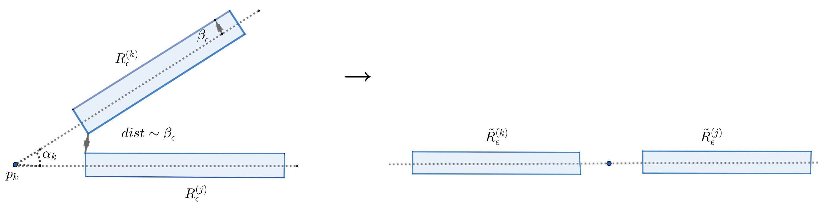
Figure 5. The transformation $T$.

Moreover, we get the estimate

$$X(R_{\epsilon}^{(k)},R_{\epsilon}^{(j)})\ \leq\ C(\Omega_{0})\int_{-\ell_{\epsilon}^{(k)}-C\beta_{\epsilon}}^{0}\int_{-\beta_{\epsilon}}^{\beta_{\epsilon}}\int_{0}^{\ell_{\epsilon}^{(j)}+C\beta\epsilon}\int_{-\beta_{\epsilon}}^{\beta_{\epsilon}}\frac{\tilde{u}^{\prime}_{\epsilon}(t)\tilde{u}^{\prime}_{\epsilon}(s)}{\sqrt{|t-s|^{2}+|x_{2}-y_{2}|^{2}}}dtdx_{2}dsdy_{2}$$ (225)

$$\leq\ C(\Omega_{0})\Big{(}\int_{-\beta_{\epsilon}}^{\beta_{\epsilon}}\tilde{u}^{\prime}_{\epsilon}(t)\ dt\Big{)}^{2}\Big{(}\int_{0}^{\ell_{\epsilon}^{(k)}+C\beta_{\epsilon}}\int_{0}^{\ell_{\epsilon}^{(j)}+C\beta_{\epsilon}}\frac{1}{x_{2}+y_{2}}dx_{2}dy_{2}\Big{)}.$$ (226)

Both integrals on the right hand side of (226) are estimated by a universal constant. For two non-adjacent edge regions one has $|x-y|=O(1)$ for $x\in R_{\epsilon}^{(k)}$ and $y\in R_{\epsilon}^{(j)}$. With an analogous transformation as before we hence have

$$X(R_{\epsilon}^{(k)},R_{\epsilon}^{(j)})\ \leq\ C(\Omega_{0})\int_{-\beta_{\epsilon}}^{\beta_{\epsilon}}\int_{-\beta_{\epsilon}}^{\beta_{\epsilon}}\tilde{u}^{\prime}_{\epsilon}(t)\tilde{u}^{\prime}_{\epsilon}(s)\ dtds\leq C(\Omega_{0}).$$ (227)

∎

In the next lemma we estimate the local term in the energy:

Lemma 3.5 (Recovery sequence – local terms).

Let $\Omega_{0}\subset Q_{\ell}$ be a polygonal set which satisfies the assumptions of Definition 3.2. Let $m_{\epsilon}\to m=(\chi_{\Omega_{0}}-\chi_{\Omega_{0}^{c}})e_{1}$ be the sequence from Definition 3.2 and let $\sigma_{\epsilon}:=\nabla\cdot(m_{\epsilon}-M)$. Then

$$\frac{1}{2}\int_{Q_{\ell}}\Big{(}\epsilon|\nabla m_{\epsilon}|^{2}+\frac{v_{\epsilon}^{2}}{\epsilon}\Big{)}\ dx\ \leq\ 2\int_{\SS_{m}}1\ dx+C(\Omega_{0})\epsilon^{\frac{5}{6}}.$$ (228)

Proof.

We use the notations of the proof of Definition 3.2. Let the edge and corner regions $R_{\epsilon}^{(k)}$ and $C_{\epsilon}^{(k)}$ be given as in the proof of Lemma 3.4. Then

$$\frac{1}{2}\int_{Q_{\ell}}\Big{(}\epsilon|\nabla m_{\epsilon}|^{2}+\frac{v_{\epsilon}^{2}}{\epsilon}\Big{)}\ dx\ =\ \frac{1}{2}\sum_{k=1}^{N}\int_{R_{\epsilon}^{(k)}\cup C_{\epsilon}^{(k)}}\Big{(}\epsilon|\nabla m_{\epsilon}|^{2}+\frac{v_{\epsilon}^{2}}{\epsilon}\Big{)}\ dx.$$ (229)

By Lemma 3.3(i), we have

$$\frac{1}{2}\int_{R_{\epsilon}^{(k)}}\Big{(}\epsilon|\nabla m_{\epsilon}|^{2}+\frac{v_{\epsilon}^{2}}{\epsilon}\Big{)}\ dx\ =\ \frac{\ell_{\epsilon}^{(k)}}{2}\int_{-\beta_{\epsilon}}^{\beta_{\epsilon}}\Big{(}\epsilon[\tilde{u}_{\epsilon}^{\prime 2}+\tilde{v}_{\epsilon}^{\prime 2}]+\frac{\tilde{v}_{\epsilon}^{2}}{\epsilon}\Big{)}\ dt\ \leq\ 2\ell_{\epsilon}^{(k)}+Ce^{-\frac{c_{0}\beta_{\epsilon}}{\epsilon}}.$$ (230)

In the corner regions $C_{\epsilon}^{(k)}$, all level sets $d_{\partial\Omega_{\epsilon}}^{-1}(s)$ have length no larger than $8\pi\beta_{\epsilon}$. Thus by the coarea formula and Lemma 3.3(i), and the choice $\beta_{\epsilon}=\epsilon^{\frac{5}{6}}$

$$\int_{C_{\epsilon}^{(k)}}\epsilon|\nabla m_{\epsilon}|^{2}+\frac{v_{\epsilon}^{2}}{\epsilon}\ dx\ \leq\ C\beta_{\epsilon}\int_{-\beta_{\epsilon}}^{\beta_{\epsilon}}\epsilon(\tilde{u}_{\epsilon}^{\prime 2}+\tilde{v}_{\epsilon}^{\prime 2})+\frac{\tilde{v}_{\epsilon}^{2}}{\epsilon}\ dt\ \leq\ C\epsilon^{\frac{5}{6}}.$$ (231)

The assertion follows by summing up the above estimates. ∎

With Lemmas 3.5–3.4 at hand, we are ready to give the proof of the limsup–inequality:

Proposition 3.6 (Limsup–inequality for $\Gamma$–limit).

For any $m\in{\mathcal{A}}_{0}$ there exists a recovery sequence $m_{\epsilon}\in{\mathcal{A}}$ with $m_{\epsilon}\to m$ in $L^{1}(Q_{\ell})$ such that $\limsup_{\epsilon\to 0}E_{\epsilon}[m_{\epsilon}]\ \leq\ E_{0}[m]$.

Proof.

Given $m\in{\mathcal{A}}_{0}$ there is a sequence of $m_{j}\in{\mathcal{A}}_{0}$ with polygonal jump set such that

$$m_{j}\to m\text{ in }L^{1}(Q_{\ell})\quad\text{ and }\quad\|\nabla m_{j}\|\to\|Dm\|\qquad\text{ as }j\to\infty,$$ (232)

cf. [35, Remark 13.13]. Since $f$ is Lipschitz continuous, by Reshetnyak’s Theorem [39] $E_{0}$ is continuous with respect to the convergence in variation of measures, i.e. $E_{0}[m_{j}]\to E_{0}[m]$, where $m_{j}$ satisfies (232). By Lemma 3.1, for each $m_{j}$, there is a sequence of magnetizations $m_{j,k}$ with polygonal jump sets whose normals satisfy $|n_{1}|\leq\lambda^{-\frac{1}{2}}$, such that $m_{j,k}\to m_{j}$ in $L^{1}(Q_{\ell})$ as $k\to\infty$ and they have the same limit energy, i.e. $E_{0}[m_{j,k}]=E_{0}[m_{j}]$ for all $k$. By a standard diagonal argument, it is then enough to construct recovery sequences $m_{j,k}^{\epsilon}$ for each $m_{j,k}$, which satisfies $\limsup_{\epsilon\to 0}E_{\epsilon}[m_{j,k}^{\epsilon}]\leq E_{0}[m_{j,k}]$.

Thus we may assume that $m=(\chi_{\Omega_{0}}-\chi_{\Omega_{0}^{c}})e_{1}$, where $\Omega_{0}$ is a polygonal set which satisfies the assertions of Lemma 3.1. Let $m_{\epsilon}=(u_{\epsilon},v_{\epsilon})$ be the sequence constructed in Definition 3.2. By application of Lemmas 3.4–3.5, we have

$$E_{\epsilon}[m_{\epsilon}]\ \leq\ 2\int_{\SS_{m}}\left(1+\lambda|n_{1}|^{2}\right)d{\mathcal{H}}^{1}+\frac{C}{|\ln\epsilon|^{\frac{1}{2}}}\ =\ E_{0}[m]+\frac{C}{|\ln\epsilon|^{\frac{1}{2}}}$$ (233)

for some $C=C(\Omega_{0},\ell,M)$. Taking the limsup for $\epsilon\to 0$ in (233) we conclude the proof. ∎

4. Solution for limit problem

In this section, we derive the solution of the limit model. More precisely, we derive the ground state energy in the subcritical ($\lambda\leq 1$) and supercritical ($\lambda>1$) case, as stated in (10) in the introduction, and provide a characterization of the corresponding minimizers:

Proposition 4.1 (Solution of limit model).

The minimal energy for $m\in{\mathcal{A}}_{0}$ is given by

$$e(\lambda)\ :=\ \min_{m\in{\mathcal{A}}_{0}}E_{0}[m]\ \ =\ \begin{cases}2(1+\lambda)\ell\qquad&\text{ for }\lambda\leq 1,\\ 4\sqrt{\lambda}\ell&\text{ for }\lambda>1.\end{cases}$$ (234)

Global minimizers are those configurations, where the jump set $\SS_{m}$ is a graph of the form $x_{1}=\gamma(x_{2})$ with normal vector $n$ (pointing outside $\{m=e_{1}\}$) satisfying

$$\min\{1,\lambda^{-\frac{1}{2}}\}\ \leq\ -n_{1}\ \leq\ 1\qquad\qquad\text{for ${\mathcal{H}}^{1}$-a.e. $x\in\SS_{m}$}.$$ (235)

Proof.

From the boundary condition (2), for every $m=(u,v)\in{\mathcal{A}}_{0}$ it follows that

$$\frac{1}{2}\int_{Q_{\ell}}e_{1}\cdot\nabla u\ d{\mathcal{H}}^{1}\ =\ -\int_{\SS_{m}}n_{1}\ d{\mathcal{H}}^{1}\ =\ \ell.$$ (236)

In the subcritical case $\lambda\leq 1$, by Hölder’s inequality and (236) we get

$$E_{0}[m]\ =\ 2\int_{\SS_{m}}\big{(}1+\lambda|n_{1}|^{2}\big{)}\ d{\mathcal{H}}^{1}\ \ \stackrel{{\scriptstyle\eqref{cons}}}{{\geq}}\ 2\left({\mathcal{H}}^{1}(\SS_{m})+\frac{\lambda\ell^{2}}{{\mathcal{H}}^{1}(\SS_{m})}\right).$$ (237)

Thus the minimum is achieved for ${\mathcal{H}}^{1}(\SS_{m})=\ell$, when $\SS_{m}$ is a single line segment from $a$ to $a+\ell e_{2}$ for some $a\in[-1,1]\times\{0\}$, and the minimal energy is $2(1+\lambda)\ell$. For $\lambda>1$ we have

$$E_{0}[m]\ =\ 2\int_{\SS_{m}}\inf_{\alpha\geq 1}\Big{[}\alpha+\frac{\lambda|n_{1}|^{2}}{\alpha}\Big{]}\ d{\mathcal{H}}^{1}\ \geq\ 4\int_{\SS_{m}}\sqrt{\lambda}|n_{1}|\ d{\mathcal{H}}^{1}\ \stackrel{{\scriptstyle\eqref{cons}}}{{\geq}}4\sqrt{\lambda}\ell.$$ (238)

Equality is achieved if and only if $-n_{1}\geq\lambda^{-\frac{1}{2}}$ ${\mathcal{H}}^{1}$-a.e. on $\SS_{m}$. This yields that $\SS_{m}$ is a single graph $x_{1}=\gamma(x_{2})$ for some function $\gamma$. ∎

Appendix A Real space representation of the stray field

We first recall the following standard representation of the homogeneous $H^{\frac{1}{2}}$–norm. We give the short proof since the constant in front of the identity is essential in our arguments:

Lemma A.1 (Finite difference representation of $H^{\frac{1}{2}}$–norm).

For $m\in H^{\frac{1}{2}}(Q_{\ell})$ we have

$$\int_{Q_{\ell}}\big{|}|\nabla|^{\frac{1}{2}}m\big{|}^{2}\ dx\ =\ \frac{1}{4\pi}\int_{Q_{\ell}}\int_{\mathbb{R}^{2}}\frac{|m(x+h)-m(x)|^{2}}{|h|^{3}}\ dhdx.$$ (239)

Proof.

Using Plancherels identity (13) and Fubini’s theorem, we obtain

$$\int_{Q_{\ell}}\int_{\mathbb{R}^{2}}\frac{|m(x+h)-m(x)|^{2}}{|h|^{3}}\ dxdh=\ \int_{Q_{\ell}}|\widehat{m}(\xi)|^{2}\int_{\mathbb{R}^{2}}\frac{|1-e^{i\xi\cdot h}|^{2}}{|h|^{3}}\ dhd\xi$$ (240)

$$=\ \int_{Q_{\ell}}|\xi||\widehat{m}(\xi)|^{2}\int_{\mathbb{R}^{2}}\frac{|1-e^{i\xi\cdot h}|^{2}}{|h|^{3}|\xi|}\ dhd\xi=\ 4\pi\int_{Q_{\ell}}|\xi||\widehat{m}(\xi)|^{2}\ d\xi.$$ (241)

The last identity follows with the change of variables $h\mapsto\frac{h}{|\xi|}$ and since $\int_{\mathbb{R}^{2}}\frac{|1-e^{ih_{1}}|^{2}}{|h|^{3}}\ dh=4\pi$ (cf. [13, (39)]). ∎

The next lemma yields another representation for the $H^{\frac{1}{2}}$–norm when $j\to-\infty$ and $k\to\infty$:

Lemma A.2 ($H^{\frac{1}{2}}$–norm vs. $H^{-\frac{1}{2}}$–norm).

For $f\in C^{\infty}_{c}(Q_{\ell};\mathbb{R}^{2})$ we have

$$\frac{1}{2}\int\!\!\!\!\int_{\tilde{Q}_{\ell}\times\tilde{P}_{\ell}}\frac{|f(y)-f(x)|^{2}}{|x-y|^{3}}\ dxdy$$ (242)

$$=\ \int\!\!\!\!\int_{\tilde{Q}_{\ell}\times\tilde{P}_{\ell}}\frac{(\nabla\cdot f)(x)(\nabla\cdot f)(y)}{|x-y|}\ dxdy\ +\int\!\!\!\!\int_{\tilde{Q}_{\ell}\times\tilde{P}_{\ell}}\frac{(\nabla\times f)(x)(\nabla\times f)(y)}{|x-y|}\ dxdy$$ (243)

$$\geq\ \frac{1}{2}\int\!\!\!\!\int_{\tilde{Q}_{\ell}\times\tilde{P}_{\ell}}\frac{(\nabla\cdot f)(x)(\nabla\cdot f)(y)}{|x-y|}\ dxdy.$$ (244)

where $\tilde{Q}_{\ell}=\mathbb{R}\times[0,\ell)$ and $\tilde{P}_{\ell}=\mathbb{R}\times[j\ell,k\ell)$ for any $j<k\in\mathbb{Z}$.

Proof.

Let $I$ (resp. $J$) be first (second) integral on the second line of (242). We recall the identity $D(\frac{z}{|z|^{3}})$ = $D^{t}(\frac{z}{|z|^{3}})$ $=$ $\frac{1}{|z|^{5}}(z^{\perp}\otimes z^{\perp}$ $-$ $2z\otimes z)$ where $z^{\perp}:=(-z_{2},z_{1})$. Integrating by parts in $x$ and $y$, since $\nabla_{z}(\frac{1}{|z|})=-\frac{z}{|z|^{3}}$ and since $\nabla(f\cdot g)=(D^{t}g)f+(D^{t}f)g$ then yields

$$I =-\int\!\!\!\!\int_{\tilde{Q}_{\ell}\times\tilde{P}_{\ell}}f(x)\cdot\frac{y-x}{|x-y|^{3}}\big{[}\nabla_{y}\cdot(f(y)-f(x))\big{]}$$ (245)

$$=-\int\!\!\!\!\int_{\tilde{Q}_{\ell}\times\tilde{P}_{\ell}}\frac{2f(x)\cdot(y-x)(f(y)-f(x))\cdot(y-x)}{|x-y|^{5}}+\frac{f(x)\cdot(y-x)^{\perp}(f(y)-f(x))\cdot(y-x)^{\perp}}{|x-y|^{5}}.$$ (246)

First integrating in $y$ then in $x$ similarly yields

$$I =\ \int\!\!\!\!\int_{\tilde{Q}_{\ell}\times\tilde{P}_{\ell}}\frac{2f(y)\cdot(y-x)(f(y)-f(x))\cdot(y-x)}{|x-y|^{5}}-\frac{f(y)\cdot(y-x)^{\perp}(f(y)-f(x))\cdot(y-x)^{\perp}}{|x-y|^{5}}.$$ (247)

Taking the sum of these two expressions, one gets

$$I =\ \int\!\!\!\!\int_{\tilde{Q}_{\ell}\times\tilde{P}_{\ell}}\frac{1}{|x-y|^{3}}\Big{(}\Big{|}(f(y)-f(x))\cdot\frac{y-x}{|y-x|}\Big{|}^{2}-\frac{1}{2}\Big{|}(f(y)-f(x))\cdot\big{(}\frac{y-x}{|y-x|}\big{)}^{\perp}\Big{|}^{2}\Big{)}.$$ (248)

Since $\nabla\times f=\nabla\cdot f^{\perp}$, the same calculation as before, replacing $f$ by $f^{\perp}$, yields

$$J\ \ =\ \int\!\!\!\!\int_{\tilde{Q}_{\ell}\times\tilde{P}_{\ell}}\frac{1}{|x-y|^{3}}\Big{(}\Big{|}(f(y)-f(x))\cdot\big{(}\frac{y-x}{|y-x|}\big{)}^{\perp}\Big{|}^{2}-\frac{1}{2}\Big{|}(f(y)-f(x))\cdot\frac{y-x}{|y-x|}\Big{|}^{2}\Big{)}\ dxdy.$$ (249)

The identity (242) follows by taking the sum of the last two equations. The inequality in (242) follows from (248). ∎

We have the following singular integral characterization for the magnetostatic energy:

Lemma A.3 (Integral representations of magnetostatic energy).

Let $\sigma\in L^{2}(Q_{\ell})$ with

$$\quad\text{with }\operatorname*{spt}\sigma\Subset Q_{\ell}\quad\text{ and }\quad\int_{Q_{\ell}}\sigma\ dx\ =\ 0.$$ (250)

Then there is a unique $q\in H^{1}(Q_{\ell};\mathbb{R}^{2})$ with $\nabla\cdot q=\sigma$ and $\nabla\times q=0$ such that

$$\int_{Q_{\ell}}\big{|}|\nabla|^{-\frac{1}{2}}\sigma\big{|}^{2}\ dx\ =\ \frac{1}{4\pi}\int_{Q_{\ell}}\int_{\mathbb{R}^{2}}\frac{|q(x+h)-q(x)|^{2}}{|h|^{3}}\ dhdx$$ (251)

$$=\ \frac{1}{2\pi}\lim_{N\to\infty,N\in\mathbb{N}}\int_{Q_{\ell}}\int_{\mathbb{R}\times[-N\ell,N\ell]}\frac{\sigma(x+h)\sigma(x)}{|h|}\ dhdx.$$ (252)

Proof.

By assumption (250) we have $\widehat{\sigma}(0)=0$ and $\nabla\widehat{\sigma}\in L^{\infty}(\mathbb{R}\times\frac{2\pi}{\ell}\mathbb{Z})$. This implies that $q\in H^{1}(Q_{\ell};\mathbb{R}^{2})$, where $q$ is defined by its Fourier transform $\widehat{q}:=-i\frac{\xi}{|\xi|^{2}}\widehat{\sigma}$. By construction $q$ satisfies $\nabla\cdot q=\sigma$ and $\nabla\times q=0$. This solution is unique by the uniqueness of the Helmholtz decomposition. By (14), since $|\widehat{\sigma}|=|\xi||\widehat{q}|$ and by (239) we then get

$$\int_{Q_{\ell}}||\nabla|^{-\frac{1}{2}}\sigma|^{2}\ d\xi\ \stackrel{{\scriptstyle\eqref{frac-sob}}}{{=}}\ \int_{\mathbb{R}\times\frac{2\pi}{\ell}\mathbb{Z}}|\xi||\widehat{q}|^{2}\ d\xi\ \stackrel{{\scriptstyle\eqref{rep-h12}}}{{=}}\ \frac{1}{4\pi}\int_{Q_{\ell}}\int_{\mathbb{R}^{2}}\frac{|q(x+h)-q(x)|^{2}}{|h|^{3}}\ dhdx.$$ (253)

Together with Lemma A.2 this yields (251). ∎

Acknowledgements: We are grateful to the referee for carefully reading the file and his useful comments. We also thank J. Fabiszisky for carefully proofreading and drawing some of the pictures. H. Knüpfer was partially supported by the German Research Foundation (DFG) by the project #392124319 and under Germany’s Excellence Strategy – EXC-2181/1 – 390900948. W. Shi was partially supported by the German Research Foundation (DFG) by the project SH 1403/1-1.

References

- [1] E. Acerbi, N. Fusco, and M. Morini. Minimality via second variation for a nonlocal isoperimetric problem. Comm. Math. Phys., 322(2):515–557, 2013.
- [2] G. Alberti and G. Bellettini. A non-local anisotropic model for phase transitions: asymptotic behaviour of rescaled energies. European J. Appl. Math., 9(3):261–284, 1998.
- [3] F. Alouges, T. Rivière, and S. Serfaty. Néel and cross-tie wall energies for planar micromagnetic configurations. ESAIM Control Optim. Calc. Var., 8:31–68 (electronic), 2002. A tribute to J. L. Lions.
- [4] L. Ambrosio, G. Da Prato, and A. Mennucci. Introduction to measure theory and integration, volume 10 of Appunti. Scuola Normale Superiore di Pisa (Nuova Serie). Edizioni della Normale, Pisa, 2011.
- [5] G. Anzellotti, S. Baldo, and A. Visintin. Asymptotic behavior of the Landau-Lifshitz model of ferromagnetism. Appl. Math. Optim., 23(1):171–192, 1991.
- [6] M. Bonacini and R. Cristoferi. Local and global minimality results for a nonlocal isoperimetric problem on . SIAM J. Math. Anal., 46(4):2310–2349, 2014.
- [7] Y. Burago and V. Zalgaller. Geometric inequalities, volume 285 of Grundlehren der Mathematischen Wissenschaften. Springer-Verlag, Berlin, 1988.
- [8] G. Carbou. Thin layers in micromagnetism. Math. Models Methods Appl. Sci., 11(09):1529–1546, 2001.
- [9] B. Cerruti and S. Zapperi. Dynamic hysteresis from zigzag domain walls: Discrete model and Monte Carlo simulations. Phys. Rev. B, 75(6), 2007.
- [10] R. Choksi and M.A. Peletier. Small volume fraction limit of the diblock copolymer problem: I. Sharp-interface functional. SIAM J. Math. Anal., 42(3):1334–1370, 2010.
- [11] R. Choksi and Mark A. Peletier. Small volume-fraction limit of the diblock copolymer problem: II. Diffuse-interface functional. SIAM J. Math. Anal., 43(2):739–763, 2011.
- [12] S. Conti, I. Fonseca, and G. Leoni. A -convergence result for the two-gradient theory of phase transitions. Comm. Pure Appl. Math., 55(7):857–936, 2002.
- [13] A. DeSimone, H. Knüpfer, and F. Otto. 2-d stability of the Néel wall. Calc. Var. Partial Differential Equations, 27(2):233–253, 2006.
- [14] A. DeSimone, R.V. Kohn, S. Müller, and F. Otto. Recent analytical developments in micromagnetics. In G. Bertotti and I. D. Mayergoyz, editors, The Science of Hysteresis, volume 2 of Physical Modelling, Micromagnetics, and Magnetization Dynamics, pages 269–381. Academic Press, Oxford, 2006.
- [15] A. DeSimone, S. Müller, R. V. Kohn, and F. Otto. A compactness result in the gradient theory of phase transitions. Proc. Roy. Soc. Edinburgh Sect. A, 131(4):833–844, 2001.
- [16] R. Engel-Herbert and D.M. et al. Schaadt. The nature of charged zig-zag domains in MnAs thin films. J. Mag. and Mag. Mat., 305(2):457–463, 2006.
- [17] I. Fonseca and C. Popovici. Coupled singular perturbations for phase transitions. Asymptot. Anal., 44(3-4):299–325, 2005.
- [18] C. Garcia-Cervera. Magnetic domains and magnetic domain walls. PhD thesis, New York University, 1999.
- [19] D. Goldman, C. Muratov, and S. Serfaty. The -limit of the two-dimensional Ohta-Kawasaki energy. Droplet arrangement via the renormalized energy. Arch. Rational Mech. Anal., 212:445–501, 2014.
- [20] S. Hamzaoui, M. Labrune, and I. Puchalska. Static and Dynamic Zig-Zag Magnetic Domains. Applied Physics Letters, 45(11):1246–1248, 1984.
- [21] A. Hubert. Charged walls in thin magnetic films. IEEE Trans. Magn., 15(5):1251–1260, 1979.
- [22] A. Hubert and R. Schäfer. Magnetic domains: the analysis of magnetic microstructures. Springer Science & Business Media, 1998.
- [23] R. Ignat and H. Knüpfer. Vortex energy and Néel walls in thin-film micromagnetics. Commun. Pure Appl. Math., 63(12):1677–1724, 2010.
- [24] R. Ignat and R. Moser. A zigzag pattern in micromagnetics. J. Math. Pures Appl. (9), 98(2):139–159, 2012.
- [25] R. Ignat and F. Otto. A compactness result in thin-film micromagnetics and the optimality of the Néel wall. J. Eur. Math. Soc., 10:909–956, 2008.
- [26] Vesa Julin and Giovanni Pisante. Minimality via second variation for microphase separation of diblock copolymer melts. J. Reine Angew. Math., 729:81–117, 2017.
- [27] B. Kaplan and R. Kaplan. Two-Dimensional Zigzag Domain Wall Structure in Ultrathin Films. Journal of Superconductivity and Novel Magnetism, 29(11):2987–2990, 2016.
- [28] H. Knüpfer and C. Muratov. On an isoperimetric problem with a competing non-local term. I. The planar case. Comm. Pure Appl. Math., 66:1129–1162, 2013.
- [29] H. Knüpfer and C. Muratov. On an isoperimetric problem with competing non-local term. II. The general case. Comm. Pure Appl. Math., 67:1974–1994, 2014.
- [30] H. Knüpfer, C. Muratov, and F. Nolte. Magnetic domains in thin ferromagnetic films with strong perpendicular anisotropy. Arch. Ration. Mech. Anal., 232(2):727–761, 2019.
- [31] R.V. Kohn and V. Slastikov. Another thin-film limit of Micromagnetics. Arch. Ration. Mech. Anal., 178(2):227–245, 2005.
- [32] L. Landau and E. Lifshitz. On the theory of the dispersion of magnetic permeability in ferromagnetic bodies. Phys. Z. Sowjetunion, 8(153):101–114, 1935.
- [33] E.H. Lieb and M. Loss. Analysis, volume 14 of Graduate Studies in Mathematics. American Mathematical Society, Providence, RI, second edition, 2001.
- [34] J.L. Lions and E. Magenes. Non-homogeneous boundary value problems and applications. Vol. I. Springer-Verlag, New York-Heidelberg, 1972. Die Grundlehren der mathematischen Wissenschaften, Band 181.
- [35] F. Maggi. Sets of finite perimeter and geometric variational problems, volume 135 of Cambridge Studies in Advanced Mathematics. Cambridge University Press, Cambridge, 2012. An introduction to geometric measure theory.
- [36] C. Melcher. The logarithmic tail of Néel walls. Arch. Ration. Mech. Anal., 168(2):83–113, 2003.
- [37] C. Melcher. Logarithmic lower bounds for Néel walls. Calc. Var. Part. Diff. Eq., 21(2):209–219, 2004.
- [38] R. Moser. On the energy of domain walls in ferromagnetism. Interfaces Free Bound., 11(3):399–419, 2009.
- [39] Y. Reshetnyak. Weak convergence of completely additive vector functions on a set. Siberian Mathematical Journal, 9(6):1039–1045, Nov 1968.
- [40] T. Rivière and S. Serfaty. Limiting domain wall energy for a problem related to micromagnetics. Comm. Pure Appl. Math., 54(3):294–338, 2001.
- [41] T. Rivière and S. Serfaty. Compactness, kinetic formulation, and entropies for a problem related to micromagnetics. Comm. Part. Diff. Eq., 28(1-2):249–269, 2003.
- [42] L Sander, R. Jones, and Collins A. An investigation of saw-tooth domain walls in ni/fe/co films. J. Phys. D, 10, 1977.
- [43] V. Ukleev and et al. Moubah, R. Imprinted Magnetic Anisotropy and Zigzag Domain Structure of Amorphous TbCo Films. J. Supercond. Novel Mag., 28(12):3571–3577, 2015.