Sparktope: linear programs from algorithms

Abstract

In a recent paper Avis, Bremner, Tiwary and Watanabe gave a method for constructing linear programs (LPs) based on algorithms written in a simple programming language called Sparks. If an algorithm produces the solution $x$ to a problem in polynomial time and space then the LP constructed is also of polynomial size and its optimum solution contains $x$ as well as a complete execution trace of the algorithm. Their method led us to the construction of a compiler called sparktope which we describe in this paper. This compiler allows one to generate polynomial sized LPs for problems in P that have exponential extension complexity, such as matching problems in non-bipartite graphs.

In this paper we describe sparktope, the language Sparks, and the assembler instructions and LP constraints it produces. This is followed by two concrete examples, the makespan problem and the problem of testing if a matching in a graph is maximum, both of which are known to have exponential extension complexity. Computational results are given. In discussing these examples we make use of visualization techniques included in sparktope that may be of independent interest. The extremely large linear programs produced by the compiler appear to be quite challenging to solve using currently available software. Since the optimum LP solutions can be computed independently they may be useful as benchmarks. Further enhancements of the compiler and its application are also discussed.

Keywords: Linear programming, polytopes, extension complexity, makespan, maximum matching

1 Introduction

Linear programming is one of the big success stories of optimization and is routinely used to efficiently solve extremely large problems. In 1982 Valiant [16] showed that any problem in P can be solved by a polynomial sized linear program (LP). His proof technique, via families of circuits, was uniform in the sense that all instances of the problem with given size $n$ can be solved by a single LP. However, for a given computational problem, the construction of such families of circuits appears quite difficult. The question of how to systematically construct these LPs lead to the recent work of Avis et al. [4] which we continue in this paper. The main contribution of [4] was to give a direct method to produce polynomial size LPs from polynomial time algorithms. Specifically they constructed LPs directly from algorithms expressed in a simple language called Sparks. The resulting LPs are uniform in the sense described above. The main purpose of the present paper is to describe the implementation of a compiler that takes Sparks code as input and produces an LP that performs the same function. We give two concrete examples of its use: the makespan problem and the maximum matching problem.

The matching problem and its relationship to the field of extension complexity was one of the main motivations of our work. A matching $M$ in an undirected graph $G=(V,E)$ with $n$ vertices is a set of vertex disjoint edges from $E$. The maximum matching problem is to find a matching in $G$ with the largest number of edges. A related decision problem is to decide if a given matching $M$ in $G$ has maximum size. Both of these problems can be solved in polynomial time by running Edmonds’ algorithm [8]. As well as this combinatorial algorithm, Edmonds also introduced a related polytope [7] which is known as the Edmonds’ polytope $\mathrm{EP}_{n}$ and whose variables correspond the the $n(n-1)/2$ edges of the complete graph $K_{n}$. Matching problems can be solved by a linear program with constraint set $\mathrm{EP}_{n}$, where the coefficients of the objective function are one for the edge set $E$ and zero otherwise. Unlike his algorithm’s polynomial running time, $\mathrm{EP}_{n}$ has size exponential in $n$. This raised the question of whether $\mathrm{EP}_{n}$ could be the projection of a higher dimensional polytope that does have polynomial size. Such a polytope is called an extended formulation and is the central concept in extension complexity (see, e.g., Fiorini et al. [9]). However, in a celebrated result, Rothvoss [14] proved $\mathrm{EP}_{n}$ admits no polynomial size extended formulation. Rothvoss’s result has sometimes been misinterpreted to mean that no polynomial sized LP exists for the matching problem. In Section 6 of the paper we give details of the construction of a uniform family of LPs for the maximum matching problem that have polynomial size.

The Sparks language was modeled on Sahni’s proof of Cook’s theorem given in [11]. Since Sparks is strong enough to implement Edmonds’ algorithm in polynomial time, it can produce the required polynomial sized LPs for the matching problem. In this paper we describe the implementation those ideas in a compiler we developed called sparktope. We then show how sparktope can be used to produce polynomial sized LPs for two problems with exponential extension complexity: makespan and maximum matching. We should emphasize here that sparktope will convert any algorithm written in Sparks  into a linear program. However this LP will only have polynomial size if the algorithm terminates in polynomial time. Nevertheless our approach gives new results even for NP-hard problems. For example, converting the Held-Karp travelling salesman algorithm [10] into an LP via Sparks gives an asymptotically smaller LP than that formed from the convex hull of the Hamiltonian circuits. This is discussed further in the concluding remarks.

The paper is organized as follows. In Section 2 we summarize the results in [4] and their main theorem. Sections 3 and 4 describe details of the Sparks compiler and how it produces linear programs. This is followed by Sections 5 and 6 which describe the application of sparktope to produce linear programs for the makespan and maximum matching problems. We give some concluding remarks in Section 7. In the appendices we give a complete Sparks code for the matching problem and a sample input.

2 Linear programs and weak extended formulations

In this section we review the results in [4] that are relevant to the present paper. The proofs for results stated here can be found in that paper. For simplicity we initially restrict the discussion to decision problems however the results apply to optimization problems also. Let $X$ denote a decision problem defined on binary input vectors $x=(x_{1},...,x_{q})$, and an additional bit $w_{x}$, where $w_{x}=1$ if $x$ results in a “yes” answer and $w_{x}=0$ if $x$ results in a “no” answer. We define the polytope $P$ as:

$$P=\operatorname{CH}\{(x,w_{x}):x\in\{0,1\}^{q}\}$$ (1)

For a given binary input vector $\bar{x}$ we define the vector $c=(c_{j})$ by:

$$c_{j}=\begin{cases}~{}~{}1&\text{if}~{}\bar{x}_{j}=1\\ -1&\text{if}~{}\bar{x}_{j}=0\end{cases}~{}~{}~{}~{}~{}~{}~{}~{}~{}~{}1\leq i<j\leq n$$ (2)

and let $d$ be a constant such that $0<d\leqslant 1/2$. We construct an LP:

$$z^{*}= \max ~{}c^{T}x+dw$$

$$s.t. ~{}(x,w)\in P$$

Proposition 1 ([4]).

For any $\bar{x}\in\{0,1\}^{q}$ let $m=\mathds{1}^{T}\bar{x}$. The optimum solution to (2) is unique, $z^{*}=m+d$ if $\bar{x}$ has a “yes” answer and $z^{*}=m$ otherwise.

We will be interested in problems where the constraint set describing $P$ has an exponential number of constraints implying that the LP (2) has exponential size. It may still be the case that $P$ is be the projection of a higher dimensional polytope $Q$ that does have polynomial size, which would give a polynomial size LP. Two examples of this are the spanning tree polytope (see Martin [13]) and the cut polytope for graphs with no $K_{5}$ minor (see, e.g., Deza and Laurent [6], Section 27.3). Such a polytope $Q$ is called an extended formulation and is the central concept in extension complexity (see, e.g., Fiorini et al. [9]). The condition that $Q$ projects onto $P$ is a strong one: there are problems in P that have exponential extension complexity. In a celebrated result Rothvoss [14] proved that the maximum matching problem in graphs was such a problem. We describe below how a weaker notion of extension complexity leads to polynomial size LPs for problems in P.

In what follows the $k$-cube refers to the $k$ dimensional hypercube whose vertices are all the binary vectors of length $k$.

Definition 1 ([4]).

Let $Q$ be a polytope which is a subset of the $(q+t)$-cube with variables labelled $x_{1},...,x_{q}$, $y_{1},...,y_{t}$. We say that $Q$ has the x-0/1 property if each of the $2^{q}$ ways of assigning 0/1 to the variables $x_{1},...,x_{q}$ uniquely extends to a vertex $(x,y)$ of $Q$ and, furthermore, $y$ is 0/1 valued. $Q$ may have additional fractional vertices.

In polyhedral terms, for every binary vector $b\in{\mathbb{R}}^{q}$, the intersection of $Q$ with the hyperplanes $x_{j}=b_{j}$ is a 0/1 vertex of $Q$. We will show that we can solve a decision problem $X$ by replacing $P$ in (2) by a polytope $Q$ based on an algorithm for solving $X$, while maintaining the same objective functions. If this algorithm runs in polynomial time then $Q$ has polynomial size. We call $Q$ a weak extended formulation as it does not necessarily project onto $P$.

Definition 2 ([4]).

A polytope

$$Q=\{(x,w,s):x\in[0,1]^{q},w\in[0,1],s\in[0,1]^{r},Ax+bw+Cs\leqslant h\}$$

is a weak extended formulation (WEF) of $P$ if the following hold:

• $Q$ has the $x$-0/1 property.

• For any vector $\bar{x}\in\{0,1\}^{q}$ let $m=\mathds{1}^{T}\bar{x}$, let $c$ be defined by (2) and let $0<d\leqslant 1/2$. If $\bar{x}$ has a “yes” answer (i.e. $(\bar{x},1)\in P$) the optimum solution of the LP

  $$z^{*}=\max~{}\{c^{T}x+dw:(x,w,s)\in Q\}$$ (4)

  is unique and takes the value $z^{*}=m+d$. Otherwise the optimal solution may not be unique but $z^{*}<m+d$.

The first condition states that any vertex of $Q$ that has 0/1 values for the $x$ variables has 0/1 values for the other variables as well. The second condition connects $Q$ to $P$. For a 0/1 valued vertex $(x,w,s)$ of $Q$ we have $w=1$ if $x$ encodes a “yes” answer since $z^{*}=m+d=\mathds{1}^{T}\bar{x}$. If $x$ encodes a “no” answer then $z^{*}<m+d$ and we must have $w=0$. The purpose of the coefficient $d$ is so that we can distinguish the two answers by simply observing the value of $z^{*}$.

In general $Q$ will have fractional vertices and that is why the condition for “no” answers differs from that given in Proposition 1. However, for small enough $d$ we can ensure that the LP optimum solution is unique in both cases and corresponds to that given in Proposition 1.

Proposition 2 ([4]).

Let $Q$ be a WEF of $P$. There is a positive constant $d_{0}$, whose size is polynomial in the size of $Q$, such that for all $d$, $0<d<d_{0}$, the optimal solution of the LP defined in (4) is unique, $z^{*}=m+d$ if $\bar{x}$ has a “yes” answer and $z^{*}=m$ if $\bar{x}$ has a “no” answer.

If we are able to observe the value of $w$ in the optimum solution of (4) then we may in fact set $d=0$. In this case $z^{*}=m$ for both answers and it follows from the 0/1 property that the optimum solution is unique and 0/1 valued. Since $Q$ is a WEF of $P$ the value of $w$ in the optimum solution gives the correct answer to the decision problem. This is the preferred method in practice as it reduces the problem of floating point round off errors which may be caused by small values of $d$.

Combining the above results with the circuit complexity model the following theorem was obtained. P/poly is the class of decision problems that can be solved by polynomial size circuits.

Theorem 1 ([4]).

Every decision problem $X$ in P/poly admits a weak extended formulation $Q$ of polynomial size.

Since constructing circuits is a cumbersome way to express algorithms the authors obtained the same result by working with algorithms expressed in pseudocode. This has the additional advantage that they could also obtain similar results for optimization problems directly, i.e. without having to resort to binary search. They chose to use the language Sparks  which is described next.

3 Sparks and its assembly language Asm

To convert an algorithm into an LP there is a trade-off between the ease of writing the algorithm in a reasonably high level language and the ease of converting a program in this language into a set of LP constraints. For this reason we follow the usual practice of introducing a programming language and converting it to an intermediate language (so-called “assembly code”) before finally converting the intermediate language into a set of LP constraints. We detail the first two steps in this section and the third step in the next section. In order to get a single LP to handle all inputs of a given size $n$ it will be necessary to get a bound on the number of steps required to complete any input of this size. Since our step clock is based on assembly instructions executed it is necessary to detail these for each high level instruction.

The language Sparks was introduced in Horowitz and Sahni [11] where it was used for a proof of Cook’s theorem that was based on pseudocode rather than Turing machines. We have implemented those features of Sparks that are necessary for expressing combinatorial algorithms such as Edmonds’ unweighted matching algorithm. Additional features would be needed to handle more sophisticated problems, such as the weighted matching problem. For further details, the reader is referred to Section 11.2 of [11].

We refer to our intermediate language Asm as an assembly code since it implements a register based virtual instruction set. Unlike a conventional compiler for a language like C or FORTRAN, most of the translation effort is actually generating the final output (in our case linear inequalities) from the Asm code. Readers familiar with virtual machine based languages like Java or Python may find it helpful to think of the generated linear constraints as implementing a virtual machine that executes the Asm instructions.

We distinguish between compile time, when the system of inequalities corresponding to a particular Sparks program is generated, and run time, when the inputs to the program are defined, and the resulting LP solved.

A Sparks program consists of a sequence of statements, where each statement is either a variable declaration, an assignment, or a block structured control statement.

• Scalar variables are binary valued or $W$-bit integers, for some $W$ fixed at compile time.

• Arrays of binary values are allowed and may be one or two dimensional. Dimension information is specified at the beginning of the program. One dimensional arrays of integers are equivalent to two dimensional binary arrays with $W$ columns.

• For an input size of $n$, we let $p(n)$ denote the maximum number of steps required for the program to complete and $q(n)$ denote the maximum number of bits required to represent all variables. Sahni argues that $q(n)=O(p(n))$, however typically $q(n)$ is significantly smaller.

• Certain variables are designated as input and used to provide input to the program at run time. All other variables are initially zero.

• An assignment has scalar variable or array reference on the left hand side, and an expression on the right hand side. A simple expression has a single operator (or is just a variable). Sparks supports a limited set of compound expressions, currently only permitting joining two simple expressions with a binary operator.

• Sparks supports block structured if, while, and for statements.

• The program terminates if it reaches a return statement, which sets a binary output variable as a side effect.

The remainder of this section gives details of the above Sparks statements along with the assembler code they generate. It is rather technical and may be skipped on first reading and referred to as necessary to understand the examples given in Sections 5 and 6.

As noted above, the number of assembler code instructions is necessary to obtain bounds on the size of the LP constraint set generated. These bounds are given for each code sample below. In these samples, $x,y,z$ are assumed declared boolean, $i,j,k$ are assumed declared integer, $A$ is a boolean array, and $B$ is an integer array.

3.1 Simple assignments

Some Sparks statements translate one-to-one to Asm statements. We group them here according to argument type.

In actual Sparks input $\leftarrow$ is typed ‘$\leftarrow$’. The Boolean equality test is written ‘=’, rather than ‘==’. The ‘.’ in the first column of the Asm is a placeholder for a statement label.

The notation B$\llbracket$i$\rrbracket$ (entered as B$\llbracket$i$\rrbracket$) indicates a row of a Boolean matrix should be interpreted as an integer.

3.1.1 Negated operators

Currently there is only one negated operator supported. It translates to two Asm statements.

3.2 Array reads

Array reads translate to one extra Asm statement (and one extra step) per array reference compared to the statements in Section 3.1.

$$\operatorname{steps}(\textsf{array using expr})=\operatorname{steps}(\textsf{basic expr})+\#(\textsf{array refs}).$$

3.3 Compound assignments

For convenience Sparks supports a single level of compound expressions as right-hand-sides. In particular any right hand side from Subsection 3.1 can be joined by an operator to any other with matching type (i.e. bool or int). The steps needed for the resulting Asm code can be calculated as follows:

$$\operatorname{steps}(\textsf{compound})=\operatorname{steps}(\textsf{rhs})+\operatorname{steps}(\textsf{lhs})+1\,.$$

3.4 if blocks

The steps required for Sparks control structures can be calculated in terms of the steps required for the controlling expression(s) and for those the body. The simplest case is the one-branched if (i.e. no else).

$$\operatorname{steps}(\textsf{if})\leq\operatorname{steps}(\textsf{body})+\operatorname{steps}(\textsf{bool\_expr})+2$$

3.5 if-then-else blocks

The if-then-else block is similar, except there are two bodies to account for, and one more overhead step.

$$\operatorname{steps}(\textsf{if-else})\leq\max\left(\operatorname{steps}(\textsf{body}_{t}),\operatorname{steps}(\textsf{body}_{f})\right)+\operatorname{steps}(\textsf{bool\_expr})+3$$

3.6 while loops

A while loop can be analysed in essentially the same was as an if block, with the both the controlling expression and the body executed one per iteration. In general (e.g. with nested loops) the cost of executing the loop body can vary between iterations: we use the notation $\operatorname{steps}(\textsf{body};i)$ to denote the number of steps to execute the body on the $i$-th iteration. The last execution of the controlling expression must be counted separately.

$$\operatorname{steps}(\textsf{while}) =\sum_{i\in\mathrm{iterations}}\left(\operatorname{steps}(\textsf{bool\_expr})+\operatorname{steps}(\textsf{body};i)+3\right)$$

$$\qquad+\operatorname{steps}(\textsf{bool\_expr})+2$$

3.7 for loops

Sparks for loops have two integer expressions defining the loop bounds, but these are only evaluated once, outside the loop. As with while loops, a careful analysis may need to distinguish between the costs of different iterations, so we again use the notation $\operatorname{steps}(\textsf{body};i)$ for the cost of the $i$th iteration of the loop body.

$$\operatorname{steps}(\textsf{for})=\operatorname{steps}(\textsf{lower})+\operatorname{steps}(\textsf{upper})+\sum_{i=\textsf{lower}}^{\textsf{upper}}\left(\operatorname{steps}(\textsf{body};i)+4\right)-2$$

Examples of Sparks code are given in Sections 5 and 6 for the makespan and maximum matching problem respectively.

4 Linear programs from Sparks

The translation of a Sparks  program into an LP is adapted from a proof of Cook’s theorem given in [11] which is attributed to Sartaj Sahni. In Sahni’s construction the underlying algorithm may be non-deterministic, but we will consider only deterministic algorithms. Furthermore, Sahni describes how to convert his pseudocode into a satisfiability expression. Although it would be possible to convert this expression into an LP, considerable simplifications are obtained by doing a direct conversion from the assembly code to an LP. We give a brief overview of the LP variables and how a simple assignment statement is implemented in inequalities in this section. Full details of this conversion along with sets of inequalities for the basic operations in Sparks were developed in [4]. Refinements were added during the implementation of the sparktope compiler and are described in the documentation at [2].

The variables in the LP are denoted as follows. They correspond to the values of variables in the source code at a given time $t$ in the execution.

• Binary variables $B(i,t),1\leqslant i\leqslant q(n),0\leqslant t<p(n)$.
  $B(i,t)$ represents the value of binary variable $i$ after $t$ steps of computation. For convenience we may group $W$ consecutive bits together as an (unsigned) integer variable $i$. $I(i,j,t)$ represents the value of the $j$-th bit of integer variable $i$ after $t$ steps of computation. The bits are numbered from right (least significant) to left (most significant), the rightmost bit being numbered 1.

• Binary arrays A binary array $R[m],m=0,1,...,u$ is stored in consecutive binary variables $B(\alpha+m,t),0\leqslant m\leqslant u,0\leqslant t\leqslant p(n)$ from some base location $\alpha$. The array index $m$ is stored as a $W$-bit integer $I(*,*,t)$ and so we must have $u\leqslant 2^{W}-1$.

• 2-dimensional binary arrays A two dimensional binary array $R[m][c]$, $m=0,1,...,u$, $c=0,1,...,v$ is stored in row major order in consecutive binary variables $B[\alpha+j,t-1]$, $0\leqslant j\leqslant uv+u+v$, $0\leqslant t\leqslant p(n)$ from some base location $\alpha$. The array indices $m$ and $c$ are stored as $W$-bit integers $I(*,*,t)$ and so we must have $u,v\leqslant 2^{W}-1$. If $v=W$, the rows of $R[m][c]$ may be addressed as $W$-bit integers.

• Step counter $S(i,t),1\leqslant i\leqslant l,1\leqslant t\leqslant p(n)$.
  Variable $S(i,t)$ represents the instruction to be executed at time $t$. It takes value 1 if line $i$ of the assembly code is being executed at time $t$ and $0$ otherwise.

All of the above variables are specifically bounded to be between zero and one in the LP. The last set of variables $S(i,t)$ encode the step counter discussed in Section 3, and are crucial to the correctness of our LPs. The step to be executed at any time $t$ will usually depend on the actual input. For each time step $t$ and Asm statement $i$ we will develop a system of inequalities which have the controlled x-0/1 property. This means they have the $x$-0/1 property (i.e. $0/1$ values of $x$ force unique $0/1$ values of the remaining variables) for some subset of variables $x$, if line $i$ is executed at time $t$. If line $i$ is not executed at time $t$ the system of inequalities for line $i$ and time $t$ is effectively redundant; more precisely the system is feasible for any vector in the corresponding $[0,1]$ hypercube. Each such set of inequalities uses $S(i,t)$ as a control variable (i.e. they are enabled if $S(i,t)=1$). This is just the usual “big-M” method where the value of $M=1$.

As an example we consider a set of constraints that corresponds to the assignment s $\leftarrow$ x xor y. Assume that $x,y,s$ are stored in $B(q,t-1),B(r,t-1),B(s,t)$ respectively.

$$S(i,t)+B(q,t-1)-B(r,t-1)-B(s,t) \leqslant 1~{}~{}~{}~{}~{}$$

$$S(i,t)-B(q,t-1)-B(r,t-1)+B(s,t) \leqslant 1~{}~{}~{}~{}~{}$$

$$S(i,t)-B(q,t-1)+B(r,t-1)-B(s,t) \leqslant 1~{}~{}~{}~{}~{}$$

$$S(i,t)+B(q,t-1)+B(r,t-1)+B(s,t) \leqslant 3~{}~{}~{}~{}~{}$$

If $S(i,t)=1$ then all constants on the right hand side are reduced by one and $S(i,t)$ can be deleted. It is easy to check the inequalities have the controlled $\{B(q,t-1),B(r,t-1)\}$-0/1 property, and that for each such 0/1 assignment $B(s,t)$ is correctly set.

We observe that each line of assembler code generates a set of constraints for each time step of the run. In many cases there may be segments of code that either cannot run after a given time step or cannot run before a given time step. A typical example of this is initialization code that is run once at the beginning and never repeated. To reduce the total number of constraints generated we introduced a compiler directed phase command. The user is required to supply in the parameter file a lower bound on the start time and upper bound on the finish time for each phase. Constraints are only generated for time steps falling inside this range. We give an example of this for the matching problem discussed in Section 6.

In order to create and solve an LP from an algorithm using sparktope three steps are required. A detailed description is given in the user’s manual available at [2] and we give only a summary here. First the algorithm is written in Sparks and a parameter file is created to define the set of instances to be solved. As a minimum this file includes the instance size, generically denoted $n$ in this paper, the number of bits $W$ required in the computation and an upper bound on the number of computational steps required to solve any instance of size $n$. Using the Sparks code and the parameter file an LP constraint set is computed for the family of inputs of size $n$. As a convenience for the programmer, arbitrary arithmetic expressions involving only parameters may be evaluated at compile time by enclosing them in $$.

The second step involves adding an objective function to this set of constraints to represent the given instance to be solved. It is important to note that the constraint set is not rebuilt for each input instance of a given size. A single constraint set is sufficient for all instances of size $n$.

Finally in the third step an LP solver is used to compute the optimum solution of the LP and hence solve the given instance. Currently glpsol (default) and cplex are supported directly. Due to variations in the LP format accepted by different solvers, we converted the compiler output to MPS before loading it with gurobi. The LPs produced by our compiler appear to be quite difficult to solve with numerical problems often encountered. For this reason an option is given to check the given LP solution using exact arithmetic (currently only supported using glpsol). Also to speed the solution we have a -f option. In this case at the second step described above in addition to inserting the objective function the $n$ input variables are set to the 0/1 values corresponding to the given instance. As proven in Proposition 2 these are their values at optimality. The job of the LP solver is to find the 0/1 values of the other variables which in turn give a full trace of the Sparks code on the given instance and hence the solution for the given instance. The LPs produced have an extremely large number of variables and this can make debugging the original Sparks code into a challenge. To assist in this process we provide a visualization of the entire run of the code based on the output of the LP solver.

In the next two sections we give two examples of algorithms converted to LPs by sparktope. The first is a simple optimization problem called makespan and the second is a decision problem to determine if a matching in a graph is maximum or not. In discussing the complexity of an LP we follow the usual practice in mixed integer programming of dropping the dependence on the word size $w$ and define it to be the number of constraints plus number of variables.

5 Makespan

The makespan problem is to schedule $m$ jobs on $n$ identical machines to minimize the finishing time, known as the makespan, of the set of jobs.

Instance

Integers $m$,$n$, and job times $p[0],\dots,p[m-1]$.

Problem

Schedule $m$ jobs on $n$ machines to minimize the latest finish time (makespan) $T$.

Output

A job schedule $x[m,n]$ where $x[i,j]=1$ if job $i$ is scheduled on machine $j$ and zero otherwise.

This problem has exponential extension complexity even when the job times are in $\{1,2\}$ and $T=2$, see Tiwary, Verdugo and Wiese [15]. We restrict ourselves to this case. It is easily seen that a greedy algorithm that schedules all the jobs with processing time 2 first and then the remaining jobs with time 1 gives the optimum schedule. This is achieved by the code ms.spk given in Figure 1. The right hand column gives the line numbers of the assembler code instructions that are generated from the source code following the descriptions given in Section 3. Due to space limitations we do not give the assembly code here but it is available at [2]. Since the processor times are either 1 or 2 the input for ms.spk can be given by specifying a boolean array p where the processing time of job $i$ is $p[i]+1,~{}i=1,2,...,n$. The variable $w$ confirms program termination, mainly for debugging.

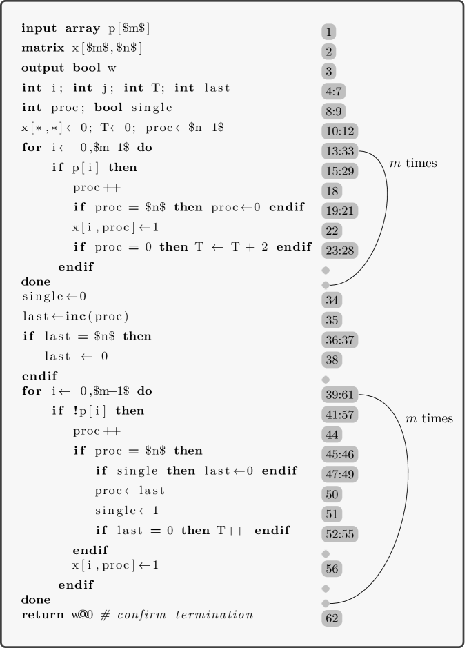
Figure 1: Sparks source code ms.spk

As written, the code requires $O(nm)$ space to hold the schedule $x$ and $O(m)$ time as it consists of two unnested for loops each run $m$ times. It follows from results in [4] that the LP produced has complexity (i.e. inequalities and variables) $O(nm^{2})$. Another implementation could use an integer array $x$ of length $m$ where $x[i]$ is the processor assigned to job $i$. Assuming $m\geq n$ the word size for integers is $O(\log m)$ and so $O(m\log m)$ space is required for $x$ and the resulting LP has complexity $O(m^{2}\log m)$. To actually produce linear programs for this problem we need to bound, for each $m$, the maximum number of assembler steps taken for any instance of this size. We do this below. For a given integer $m$ we will give an upper bound on the number of assembler code steps in order to reach a return statement. For this discussion we will refer to Figure 1, where the range of assembly lines corresponding to each Sparks line is given.

The first 9 lines are variable declarations and are not executed, so there are 53 lines of executable Asm code. We see there are two unnested for loops each executed $m$ times. The first has 19 lines (lines 15-33) and the second has 21 lines (lines 41-61). So an upper bound on number of steps executed is $53+40(m-1)=40m+13$. However inspecting the two for loops we see that they have mutually exclusive if statements depending on the value of the input $p[i]$. The body of these if statements are contained between lines 18-28 and 44-55, respectively, and only one of these blocks can be executed for each $i$. The shorter first block contains 11 statements so we may reduce the overall running time by $11m$ obtaining the upper bound $29m+13$ for the number of assembler steps executed. A slightly tighter analysis is possible by observing that some of the assembly statements for a for loop are executed only once.

An example input ms10 is provided for the case $m=10,n=3$. The Sparks input is:

                  array p[10] <- {0, 1, 1, 0, 0, 1, 1, 0, 0, 0}

The list decreasing algorithm first schedules the jobs with processing time 2, as shown on the left in Figure 2. The optimal schedule is shown on the right and has makespan $T=5$. A complete trace of the run is given in Figure 3. It shows which line is executed at each time step. This is achieved by observing in the LP optimum solution for each time $t$ the unique value of $i$ for which $S(i,t)$=1. We see that the run terminated at around time $t=245$ at the return statement in the last line of code. This termination time compares with the upper bound of $29*10+13=303$ steps calculated above. In the trace it can clearly be seen how at around $t=125$ the code switches from scheduling the jobs with processing time 2 to those with time 1.

(a) Timestep $125$

(b) Timestep $250$

Figure 2: Greedy construction of schedule from input ms10

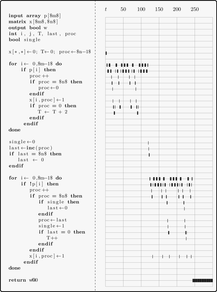
Figure 3: Trace of run on input ms10

Linear Programs							Solvers			Outputs
name	m	max	rows	columns	non-zeros	file	glpsol	cplex	gurobi	T	steps
		steps	($\times{}1000$)	($\times 1000$)	($\times 1000$)	MB
ms5	5	201	129	28	43	7	0.1	0.1	0.3	3	134
ms10	10	321	380	59	1,305	21	0.4	0.3	(31)	5	244
ms20	20	631	1,170	149	4,160	66	1.2	0.8	(91)	10	483
ms40	40	1251	3,845	412	14,099	226	3.9	2.8	(107)	20	958
ms80	80	2491	13,483	1,251	50,635	833	15	10	(587)	39	1899
ms160	160	4971	49,869	4,151	190,407	3287	55	61	(4422)	78	3790

Table 1: Makespan problem sizes, run times in seconds, computed makespan and steps to compute. (secs) indicates non 0/1 solution

Table 1 shows some test results on makespan problems for $m=5,10,20,40,80,160$ with $n=3$. The corresponding LPs (solver inputs) are available from [3].

The first 6 columns describe the linear programs generated for various values of $m$, the number of processes. They give the number of rows and columns in each LP and its size in MB using cplex LP format. The step bound is the upper bound of $31m+11$ on the number of steps required to reach a return statement, computed above. Therefore these LPs will solve any instance of the given size $m$ by simply changing the objective function. As $m$ doubles we can see the input size goes up a little less than 4 times, indicating the predicted quadratic behaviour (since $n$ was held constant). We used three solvers, glpsol 4.55, cplex 12.6.3 and gurobi 8.1.1 each with default settings. In order to use gurobi we converted all files to the larger MPS format using glpsol. Without fixing the input variables to their given 0/1 values via the -f option described earlier, all solvers gave fractional non-optimal solutions. With the input variables fixed glpsol and cplex correctly found the optimum 0/1 solution in each case using preprocessing. However gurobi could only find a 0/1 solution for $m=5$ and found fractional solutions for the other cases. The final two columns describe the outputs obtained on a test problem for each LP: the makespan $T$ and the actual number of steps executed to reach the return statement.

6 Maximum matching

We consider the following matching problem:

Instance

Integer $n$, graph $G$ and matching $M$ in $G$.

Problem

Decide whether $M$ is a maximum matching, and if it is not, to find an augmenting path.

Output

$w=0$ if $M$ is a maximum matching $w=1$ if there is an augmenting path

This standard formulation of this problem has exponential extension complexity, as follows from the result of Rothvoss [14]. However, one iteration of Edmonds’ blossom algorithm [8] can answer the above problem and this is achieved by the code mm.spk given in Appendix A. It is based on the pseudocode in [17] and a detailed explanation and proof of correctness is given in Section 16.5 of Bondy and Murty [5]. Due to space limitations we do not give the assembly code mm.asm here but it is available at [2]. As with the Makespan example we have added the relevant assembly code line numbers to the Sparks code.

To produce linear programs for this problem we need to bound, for each $n$, the maximum number of assembler steps taken for any instance size $n$. We do this in the next section getting an upper bound of less than $31n^{3}$ steps. Since the space required is $O(n^{2}\log n)$ it follows from results in [4] that the LP produced has $O(n^{5}\log n)$ constraints.

6.1 Step count analysis

For a given integer $n$ we will give an upper bound on the number of steps taken in order to reach a return statement. Referring to the source code mm.spk we see that the program is divided into two phases to reduce the number of constraints produced. phase init handles initialization and is executed once whereas phase main performs the blossom algorithm.

The loop structure of phase init is shown in Figure 4. The line numbers correspond to the assembly code mm.asm and as the first 28 lines are declarations they are omitted. It is necessary to get both an upper and lower bound on the number of steps executed in phase init. A total of 7 lines are executed once: 29-32, 38-39, and 59. The first for loop in lines 33-38 has 6 steps but the done statement is only executed once and steps 36 and 37 are executed $n-1$ times. So this loop requires exactly $5n-1$ steps. For simplicity in what follows a for loop with $k+1$ steps, including the done statement, is assigned an upper bound of $kn$ steps and a lower bound of $(k-1)n$ steps.

There remain two nested for loops in lines 20-59. The inner for loop in lines 42-54 is executed $n-1$ times with the corresponding number of iterations $=n-1,n-2,...,1$. Since the loop has 13 lines an upper bound on the number of steps executed is therefore $12(n-1+n-2+...+1)=6n(n-1)$. The remaining 7 lines in the outer for loop 40-58 contribute at most $7n$ steps. In total we have an upper bound of $7+6n^{2}-6n+7n=6n^{2}+n+1$ for phase init.

For the lower bound we note that lines 47,48 are executed only for edges in an input matching and there may be zero of those. So we reduce the size of the inner loop by 3 getting a lower bound of $9n(n-1)/2$ steps. For the outer loop we reduce its size to 6 so in total the lower bound is $7+9n(n-1)/2+6n=(9n^{2}+3n+14)/2$ steps.

For $n=8$ we have an upper bound of 393 and a lower bound of 307 steps. Referring to the output snapshot in Figure 8 we see that S[59,364]=1 and S[62,365]=1 so that for this input 364 steps were executed in phase init.

Figure 4: Control structure of phase init of mm.spk

Figure 5: Control structure of phase main

Figure 6: Control structure of path and blossom processing

We now turn to the main part of the blossom algorithm and give the control structure in Figure 5. There are three nested while loops labelled A,B,C respectively. The outer Loop A, lines 62-257, finds either an augmenting path or a blossom. A blossom is an odd cycle of length at least three which is shrunk to a single vertex, removing at least 2 nodes of the graph. Graphs cannot be shrunk to less than 3 vertices, so shrinking can happen at most $(n-3)/2$ times and this is a bound on the number of times Loop A can be executed. Loop B, lines 85-255 is executed for each vertex in the (possibly shrunk) graph, so $n$ times at most for each iteration of Loop A. Loop C, lines 100-247, is the third nested loop, and is executed at most once for each vertex adjacent to the vertex chosen in Loop B. So at most $n$ iterations are required for each iteration of Loop B.

We begin by analyzing the inner Loop C. The block of code (line numbers 133-238) shown in Figure 6 either finds an augmenting path or handles blossom shrinking. It can be executed at most once for each iteration of Loop A, so $(n-3)/2$ times in total. It is analyzed separately below. Removing these 106 lines from the 148 lines in Loop C leaves 42 lines that require at most $42n$ time steps for each iteration of Loop B. Moving to Loop B and we find 23 lines (85-99, 248-255) which are not in Loop C. Loop B executes $n$ times for each iteration of Loop A and so requires at most $42n^{2}+23n$ time steps for such an iteration.

Finally in Loop A there is a for statement, lines 68-82, executed $n$ times for a total of at most $15n$ steps per iteration. There remain 10 lines (62-67, 83-84, 256-57) executed once for each iteration. So adding in the steps for the inner loops (except shrinking) an iteration of Loop A requires at most $42n^{2}+38n+10$ steps.

We now turn to the code in Figure 6 which is executed at most $(n-3)/2$ times. Consider a single iteration of these 106 lines. Loops D and E of 7 lines each can be executed at most $n$ times each for a total of $14n$ steps. Inside the else clause beginning on line 155 are several more loops. Loop F, lines 157-165, is executed at most $n$ times for a total of $9n$ steps. Loop G, lines 169-236, is more complex. Consider a single iteration. There are two further while loops, Loop H on lines 196-213 and Loop I on lines 214-233. Since $j$ increments every time H of I runs, together these are executed at most $n$ times in an iteration of Loop G. The second of these is longer and has 20 lines. So both loops together take at most $20n$ steps for each of at most $n$ iterations, or $20n^{2}$ steps in total. The remaining 30 lines (169-195, 234-236) of Loop G are executed once per iteration. The total number of steps taken in Loop G for a single blossom shrinking is therefore at most $20n^{2}+30n$. In this code block there remain lines 141, 149-156, 166-168, 238, or a total of 12 lines, each of these is executed once per iteration of the code block. It follows that the total number of steps taken in blossom shrinking is at most $(14n+9n+20n^{2}+30n+12)=20n^{2}+53n+12$.

Putting everything together the total number of steps for an iteration of Loop A is at most $62n^{2}+91n+22$. Since this loop executes at most $(n-3)/2$ times this gives an upper bound of $(62n^{3}-75n^{2}-251n-66)/2$ steps. To this we add the upper bound on the steps taken in phase init, derived above, of $6n^{2}+n+1$ obtaining a total of $(62n^{3}-63n^{2}-249n-64)/2$ steps.

6.2 Examples

Two example inputs are provided in Appendix B for the case $n=8$, wt8 and wt8a. The graphs have vertices labelled 0,1,…,7 and the input matching has 3 edges (0,1),(2,3),(4,5) as shown for $wt8$ in Figure 7 (a). LPs (solver inputs) discussed in this section can be downloaded from [3].

(a) Graph and matching

(b) Blossom 456 found

(c) Blossom shrunk to 5

(d) No augmenting path

Figure 7: Processing the graph wt8

A snapshot of this run is given in Figure 8. We see that it terminates at a return statement on line 258 at around time 1700 indicating that an augmenting path was not found. The step count compares with the upper bound of 8123 steps calculated above.

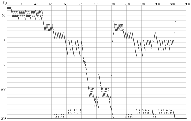
Figure 8: wt8: no augmenting path

In Figure 7(b) we see how the algorithm first finds a blossom on vertices 4,5,6 and shrinks it to vertex 5 as in Figure 7(c). In the subsequent iteration no blossom or augmenting path is found, as shown in Figure 7(d), to the run terminates.

The input wt8a contains the additional edge 47. As before a blossom on vertices 4,5,6 is found and shrunk to vertex 5. However this time an augmenting path 57 is found in the shrunk graph. This expands to the augmenting path 6,5,4,7 in wt8a. Observing the snapshot in Figure 9 we see that the run halts on line 152 of the code after about 1480 steps and returns $w=1$.

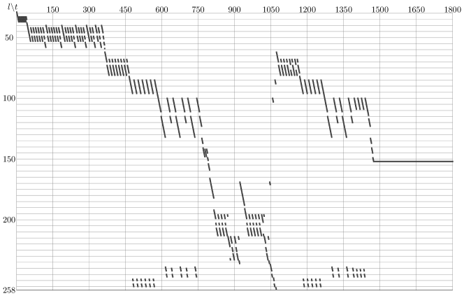
Figure 9: wt8a: augmenting path found

name	n	max steps	main.LB	init.UB	rows	columns	non-zeros	GB
mm8	8	4000 (9747)	307	393	25,490,809	2,567,920	80,568,489	1.6 (3.4)
mm10	10	7000 (19629)	472	611	54,809,388	5,354,967	210,572,706	3.6 (11)
mm12	12	10000 (34771)	673	877	94,860,776	8,200,011	371,213,800	6.3 (23)
mm16	16	16000 (83003)	1183	1553	238,577,463	15,296,088	955,445,591	15 (80)

Table 2: Linear programs generated for maximum matching

Inputs				glpsol	cplex	Outputs
name	n	m	M	secs	secs	answer	steps
wt8.in	8	15	3	32	27	max	1692
wt8a.in	8	16	3	37	26	aug	1474
wt10.in	10	19	4	98	240	max	1627
tr10.in	10	14	4	97	272	aug	3733
wt12.in	12	24	5	188	319	max	2671
tr12.in	12	17	5	189	420	aug	5295
wt16.in	16	43	7	-	1353	max	4241
tr16.in	16	23	7	-	1956	aug	9211

Table 3: Maximum matching test results

Figure 10: trn.in

Table 2 shows some statistics about linear programs built for the maximum matching problem. These are much bigger LPs than those generated for the makespan problem and the analysis of the worst case run time given above is quite loose. To make it easier for the solvers we generated LPs with a time bound somewhat less than the proven worst case. The time bounds used are shown in column 3 with the worst case bound in parenthesis. The phase bounds in columns 4 and 5 are as given above and the corresponding statistics of the LP generated are given in the next 3 columns. The disk space required to store the LP is given in the final column with the size of the LP for the proven time bound in parentheses.

Table 3 shows the results of solving the LPs for some given input graphs. Here $n$ denotes the number of vertices, $m$ the number of edges and $M$ the size of the given matching to test for being of maximum size. The graphs wtn.in derive from Tutte’s theorem and have no maximum matching, so no augmenting path is found. The graphs trn.in shown in Figure 10 achieve the maximum number, $(n-2)/2$ of shrinkings, successively matching edges (1,2),(3,4),…,$n-3,n-4$, before finding an augmenting path from vertex 0 to vertex $n-1$. We observe that the steps used in finding the solution, shown in the final column, are significantly smaller than the time bounds given in column 3 of Table 2. We used the same solvers and default settings as before, except glpsol at version 4.60 (instead of 4.55). glpsol has a limit of $10^{8}$ constraints and so was not able to handle mm16. Both cplex and glpsol solved all problems using the presolver only. gurobi was not able to solve any of the models in the presolver and produced incorrect non integer solutions after pivoting.

7 Concluding remarks

Extension complexity initially was concerned with giving exponential lower bounds for LP formulations of NP-hard problems that project onto their natural formulations. The main examples being the travelling salesman problem and the max-cut problem. These results are independent of the ${\textsc{P}}~{}\neq~{}{\textsc{NP}}$ conjecture. Later work showed that similar results also applied to some problems in P. The makespan and maximum matching problems are two examples of this. Since we know that polynomial size LPs exist for these problems, it is natural to wonder how to construct them and what their minimum size is. The sparktope project was motivated by these questions. The LPs it produces are surely not minimal. However, for example, is it possible to find an LP to solve the maximum matching problem considered here which has $o(n^{5})$ constraints?

Although we have concentrated on converting algorithms for problems in P into polynomially sized LPs the method and software described here will work for any algorithm that can be expressed in Sparks. For example, consider the travelling salesman problem. The convex hull of all TSP tours in the complete graph $K_{n}$ is called the TSP polytope. It is known that this polytope has more than $n!$ facet defining inequalities (see, e.g., [1]). However a dynamic programming algorithm due to Held and Karp [10] runs in $O(2^{n}n^{2})$ time and $O(2^{n}n)$ space. So the LP formulation produced by sparktope based on this algorithm has size $O(4^{n}n^{3}\log n)$ which is asymptotically smaller than the one based on the TSP polytope. Is there an asymptotically smaller sized LP that can solve the travelling salesman problem?

Appendix A mm.spk : sparks code

Appendix B Sample inputs for maximum matching

References

- [1] D.L. Applegate, R.E. Bixby, V. Chvatal, and W.J. Cook, The Traveling Salesman Problem: A Computational Study (Princeton Series in Applied Mathematics), Princeton University Press, 2007.
- [2] D. Avis and D. Bremner, Sparktope, http://doi.org/10.5281/zenodo.3818420, https://gitlab.com/sparktope/sparktope and http://www.cs.unb.ca/~bremner/research/sparks_lp/ (2020).
- [3] D. Avis and D. Bremner, Sparktope example LPs, https://doi.org/10.5281/zenodo.3830794 (2020).
- [4] D. Avis, D. Bremner, H.R. Tiwary, and O. Watanabe, Polynomial size linear programs for problems in P, Discrete Applied Mathematics 265 (2019), pp. 22–39.
- [5] J. Bondy and U. Murty, Graph Theory, 1st ed., Springer, 2008.
- [6] M.M. Deza and M. Laurent, Geometry of cuts and metrics, Algorithms and Combinatorics Vol. 15, Springer-Verlag, 1997.
- [7] J. Edmonds, Maximum matching and a polyhedron with vertices, J. of Res. the Nat. Bureau of Standards 69 B (1965), pp. 125–130.
- [8] J. Edmonds, Paths, trees, and flowers, Canad. J. Math. 17 (1965), pp. 449–467.
- [9] S. Fiorini, S. Massar, S. Pokutta, H.R. Tiwary, and R. de Wolf, Exponential lower bounds for polytopes in combinatorial optimization, J. ACM 62 (2015), pp. 17:1–17:23.
- [10] M. Held and R.M. Karp, A dynamic programming approach to sequencing problems, Journal of the Society for Industrial and Applied Mathematics 10 (1962), pp. 196–210.
- [11] E. Horowitz and S. Sahni, Fundamentals of Computer Algorithms., Computer Science Press, 1978.
- [12] M. Manser (2020). Private Communication.
- [13] R.K. Martin, Using separation algorithms to generate mixed integer model reformulations, Oper. Res. Lett. 10 (1991), pp. 119–128.
- [14] T. Rothvoss, The matching polytope has exponential extension complexity, J. ACM 64 (2017), pp. 41:1–41:19.
- [15] H.R. Tiwary, V. Verdugo, and A. Wiese, On the extension complexity of scheduling polytopes, Operations Research Letters 48 (2020). Available at https://doi.org/10.1016/j.orl.2020.05.008, http://arxiv.org/abs/1902.10271.
- [16] L.G. Valiant, Reducibility by algebraic projections, Enseign. Math. (2) 28 (1982), pp. 253–268.
- [17] Wikipedia contributors, Blossom algorithm, https://en.wikipedia.org/wiki/Blossom_algorithm (2009).