An Application of Quantum Annealing Computing to Seismic Inversion

Abstract

Quantum computing, along with quantum metrology and quantum communication, are disruptive technologies that promise, in the near future, to impact different sectors of academic research and industry. Among the computational challenges with great interest in science and industry are the inversion problems. These kinds of numerical procedures can be described as the process of determining the cause of an event from measurements of its effects. In this paper, we apply a recursive quantum algorithm to a D-Wave quantum annealer to solve a small scale seismic inversions problem. We compare the obtained results from the quantum computer to those derived from a classical algorithm. The accuracy achieved by the quantum computer is at least as good as that of the classical computer.

———————————————————————– ———————————————————————–

I Introduction

Seismic geophysics relies heavily on subsurface modeling based on the numerical analysis of data collected in the field. The computational processing of a large amount of data generated in a typical seismic experiment can take an equally large amount of time before a consistent subsurface model is produced. Electromagnetic reservoir data, like CSEM (Controlled Source Electromagnetic), petrophysical techniques, such as electrical resistivity and magnetic resonance on multi-wells, and engineering optimization problems like reservoir flux simulators, well field design and oil production maximization also need a strong computational apparatus for analysis.

On the other hand, in the past decade, there has been much progress in the development of quantum computers: machines exploiting the laws of quantum mechanics to solve hard computational problems faster than conventional computers. A concrete example of such progress is the so-called quantum supremacy, that has been recently demonstrated using specific purpose quantum computers Arute et al. (2019); Zhong et al. (2020); et. al. (2021). The Geoscience field and related industries, such as the hydrocarbon industry, are strong candidates to benefit from those advances brought by quantum computing.

Currently, different quantum technologies and computational models are being advanced. Giant companies like IBM, Google, and Intel are developing quantum computers based on superconducting technologies Kjaergaard et al. (2020). Other companies are also putting considerable effort into building a fully functional quantum computer based on Josephson junctions, such as the North American Rigetti, whereas, the also American IonQ and the Austrian AQT are working on computers based on trapped ions Bruzewicz et al. (2019). The Canadian company D-Wave, leader in the computational model known as quantum annealing Job and Lidar (2018), is already trading quantum machines, and the also Canadian Xanadu is providing cloud access to their photonic quantum computer Bourassa et al. (2021); Brod et al. (2019). Recent reviews comparing superconducting and trapped-ion technologies and different cloud-based platforms can be found in references Linke et al. (2017) and Devitt (2016), respectively.

In the field of Geoscience, recent works have used quantum annealers to hydrology inversion problems O’Malley (2018); Golden and O’Malley (2021). In those works, it was shown that, although the size of the problem that can be solved on a third-generation D-Wave quantum annealer is considered small for modern computers, they are larger than the problems solved with similar methodology with Intel’s third and fourth generation chips. It is also important to mention that optimization techniques are widely used in seismic inversions, but usually classical algorithms get stuck in local minima. Previous works Alulaiw and Sen (2015); Wei et al. (2006); Greer and Malley (2020) have indicated that quantum annealing can be advantageous to solve seismic problems. However, the potential applications of quantum computing in Geoscience has so far been largely unexploited in the specialized literature.

In this work, we present a formulation of a seismic problem as a binary optimization, and one small scale subsurface seismic problem is solved using the D-Wave quantum annealer available in the Amazon Braket service. We have evaluated the performance of the quantum computer comparing the results obtained to those derived from a classical computer. Our analysis was focused on the accuracy. It was found that the accuracy achieved by the quantum computer is at least as good as that of the classical computer for the problem we have studied.

This paper is organized as follows. In Sec. II we introduce the basic idea of quantum annealing. In Sections III and IV, we present the formulation of a seismic inversion as a binary optimization problem and the methods used, respectively. In Sec V, the results obtained in the D-Wave quantum annealer are shown. In the last section, we draw the conclusions.

II Quantum Annealing

In the literature, there are many different quantum computational models developed. Currently, three main models of quantum computing are being considered: the logic gate model, or circuit model, boson sampling and the adiabatic model. The gate model is an universal quantum computation model that is performed programming a step-by-step instruction build from basic building blocks, known as quantum gates, similar to the classical circuit model Nielsen and Chuang (2001). This model is exploited by companies such as IBM, Intel, Rigetti, IonQ, AQT, and Google. Boson sampling computers consists in sampling from the output distribution of bosons in a linear interferometer Aaronson and Arkhipov (2011); Brod et al. (2019). There is strong evidence that such an experiment is hard to be simulated in classical computers, but it is efficiently solved by special purpose photonic chips. The adiabatic computation model Farhi et al. (2001); Albash and Lidar (2018a) is a model in which the computational problem is mapped into a Hamiltonian, in such a way that the solution of the computational problem is encoded in the ground state of the quantum system represented by the Hamiltonian $H_{final}$. The computation is performed starting from the ground state of a known Hamiltonian $H_{initial}$. The Hamiltonian is slowly modified towards to the target Hamiltonian $H_{final}$. During the process, the total Hamiltonian of the system is given by

$$H(p)=(1-p)H_{initial}+pH_{final},$$ (1)

where $p\in[0,1]$. According to the adiabatic theorem, if the evolution is performed adiabatically, the quantum state of the system remains in the instantaneous ground state throughout the entire process.

The adiabatic model is equivalent to the gate model Aharonov et al. (2007), i.e., any problem that can be computed in the gate model will also be computable in the adiabatic model. This statement is valid for certain types of $k-$local Hamiltonians Aharonov et al. (2007). For example, considering a system of $n$ qubits, we can perform universal adiabatic computation by choosing Biamonte and Love (2008)

$$H_{initial} = \sum_{i}\delta_{i}\sigma_{i}^{x},$$ (2)

$$H_{final} = \sum_{i}H_{i}\sigma_{i}^{z}+\sum_{j>i}J_{i,j}\sigma_{i}^{z}\sigma_{j}^{z}+\sum_{j>i}K_{i,j}\sigma_{i}^{x}\sigma_{j}^{x},$$ (3)

where $\sigma_{i}^{k}$, with $k=x,y,z$, is one of the Pauli matrices of the $i^{th}$ qubit, $\delta_{i}$ and $H_{i}$ are local transverse and longitudinal fields, respectively, and $J_{i,j}$ and $K_{i,j}$ are coupling constants.

The adiabatic model can be viewed as a special case of the quantum annealing computing. In quantum annealers, the Hamiltonian change is not adiabatic. Therefore, quantum annealing is a heuristic type of computation. The D-Wave computer is a quantum annealer that uses Ising chains

$$H_{final} = \sum_{i}H_{i}\sigma_{i}^{z}+\sum_{j>i}J_{i,j}\sigma_{i}^{z}\sigma_{j}^{z}.$$ (4)

The quantum annealing performed with Ising chains is unlikely to implement universal quantum computation Preskill (2018). Therefore, D-Wave annealers are more restrictive than the universal adiabatic model. Quantum annealing with Ising chains can be applied to a class of computational problems known as NP-hard problems Barahona (1982). It is believed that quantum annealing will be able to find better approximate solutions or find such approximate solutions faster then classical computers Preskill (2018). Here, it is also important to mention that the advantage of quantum annealers over classical methods is still under debate Ronnow et al. (2014); Mandra et al. (2016); Katzgraber et al. (2015). Recent works have proposed that, in some cases, quantum annealing is advantageous over classical computing Albash and Lidar (2018b); Denchev et al. (2016); Li et al. (2018); Baldassi and Zecchina (2018), on the other hand, no advantage was reported in references Ronnow et al. (2014); Hen et al. (2015). The origin of the possible speedup is also under debate. Quantum tunneling is often claimed to be the key mechanism underlying possible speedups of quantum annealing. However, recent work has found numerical evidence that quantum tunneling processes can be efficiently simulated by Monte Carlo methods Brady and van Dam (2016) . There is also evidence to suggest that it is unlikely to achieve exponential speedups over classical computing solely by the use of quantum tunneling Crosson and Harrow (2016). The role of the temperature in the performance of quantum annealing has been also studied in Jiang et al. (2017).

To solve a problem in the D-Wave quantum annealer Job and Lidar (2018), it is necessary first to express the problem to be solved as an Ising problem or as a quadratic unconstrained binary optimization (QUBO), which is equivalent to Ising but defined on the binary values $0$ and $1$, whereas the Ising problem is defined on the binary values $\pm 1/2$. The QUBO problem can be written as the minimization of the quadratic function

$$f(\mathbf{q})=\mathbf{q}^{\mathsf{T}}\mathbf{Qq},$$ (5)

where $\mathbf{q}\in\{0,1\}^{n}$, $\mathbf{Q}$ is a $n\times n$ upper (lower) triangular matrix and the vector $\mathbf{q}^{\mathsf{T}}=(q_{1},q_{2},\cdots,q_{n})$ contains $n$ binary variables. QUBO problems are commonly used in machine learning and many important computational problems can be translated to a QUBO formulation as well Lucas (2014). Examples of problems that have been addressed with a D-Wave quantum annealer are: the classification of human cancer types Li et al. (2021), traffic optimization Neukart et al. (2017), transcription factor DNA binding Li et al. (2018), metamaterial designing Kitai et al. (2020) and Higgs boson data analysis Mott et al. (2017).

Recently, there has been a growing interest in quantum algorithms for systems of linear equations, $\mathbf{Ax=b}$, where $\mathbf{A}$ is a $n\times n$ matrix and $\mathbf{b}$ is a unit vector. Such algorithms may find applications in different research areas, including Geoscience. In the quantum gate model, the quantum version of such problem is called Quantum Linear Systems Problem (QLSP) Duan et al. (2020); Dervovic et al. (2018), and it is defined as the problem of preparing the state

$$|\psi\rangle=\frac{\sum_{i}^{n}x_{i}|i\rangle}{\sqrt{\sum_{i}^{n}|x_{i}|^{2}}},$$ (6)

where $\mathbf{x}=(x_{1},x_{2},\cdots)^{\mathsf{T}}$ is the solution of $\mathbf{Ax=b}$.

In 2008, Harrow, Hassidim, and Lloyd (HHL) proposed a quantum algorithm for the QLSP problem Harrow et al. (2009). Given some assumptions Aaronson (2015), the run time of HHL is $O(k^{2}s^{2}\log(n)/\epsilon)$ where $k$ is the condition number of the matrix $\mathbf{A}$, defined as the absolute value of the ratio between the largest and smallest eigenvalues of $\mathbf{A}$, $s$ is the sparsity of $\mathbf{A}$, defined as the number of nonzero entries per row, and $\epsilon$ is the desired precision.

After the initial HHL proposal, several improvements were achieved: the condition number dependence was reduced from $k^{2}$ to $k\log^{3}(k)$ Ambainis (2012), the error dependency was reduced from $1/\epsilon$ to a polynomial function in $log(1/\epsilon)$ Childs et al. (2017), and a sparsity-independent runtime scaling was achieved in Wossing et al. (2018). The QLSP problem can also be solved using iterative quantum solvers in runtime $O(k^{2}\log(k)/log(1/\epsilon))$ Shao and Xiang (2020) and with runtimes $O(k\log(k)/\epsilon)$ and $O(k^{2}\log(k)/\epsilon)$ using the evolution randomization method, a simple variant of adiabatic quantum computing where the parameter $p$ in (1) varies discretely, rather than continuously Subasi et al. (2019). The best general-purpose classical conjugate gradient algorithm to solve $\mathbf{Ax=b}$ has the runtime $O(nks\log(1/\epsilon))$. Here, we must emphasize a fundamental difference between classical and quantum algorithms. While the conjugate gradient returns the solution vector $\mathbf{x}$, quantum algorithms return a quantum state, equation (6), that approximately contains all the components $x_{i}$ of the solution vector $\mathbf{x}$. It is possible to obtain any specific entry $x_{i}$ by measuring the output state (6), but in general, it will require repeating the algorithm many times, which would kill the exponential speedup. Still, quantum algorithms can be used as subroutines in different applications Aaronson (2015); Duan et al. (2020).

In quantum annealers, the problems of solving a system of linear equations and a system of polynomial equations were previously studied in Rogers and Singleton (2020); Borle and Lomonaco (2019); O’Malley and Vesselinov (2016) and Chang et al. (2019), respectively. Unlike the previously mentioned quantum algorithms, quantum annealing solves $\mathbf{Ax=b}$ completely, i.e., it returns the vector $\mathbf{x}$. To compare the performances of a quantum annealer and a classical computer, we must take into account the cost to prepare the problem, i.e., the procedure to map $\mathbf{Ax=b}$ into a QUBO or Ising problem, the cost to perform the annealing, and also the cost to post-process the results. The performance of quantum annealers to solve linear systems was studied in detail in reference Borle and Lomonaco (2019). It was shown that quantum annealers might be competitive if there exists a post-processing method that is polynomial in the size of the Matrix $\mathbf{A}$ with a degree less then 3.

III Seismic Inversion written as a QUBO problem

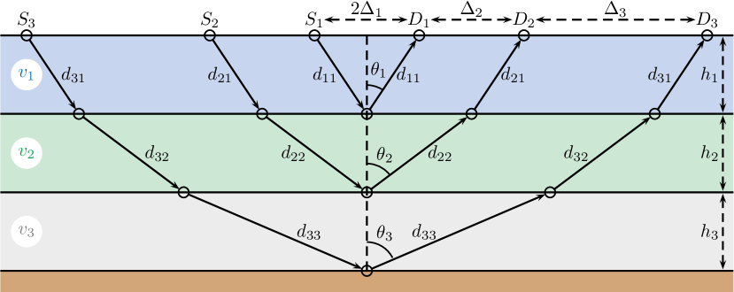
Figure 1: Schematics of seismic data acquisition. Sound traces created in the $i^{th}$ source $S_{i}$ are detected at $D_{i}$ after the time of travel $t_{i}$. This figure depicts a simplified scheme with only $m=3$ layers, but we have considered up to $m=46$.

We considered the propagation of sound waves in a multi-layered medium, as shown in Figure 1. Multiple sources produce sound waves that can be reflected in the interface of each layer. Assuming that the wave propagation can be modeled as narrow beams or rays, the sound trace originated in the $i^{th}$ source reaches the $i^{th}$ detector after the time interval

$$t_{i}=2\sum_{j=1}^{i}\frac{d_{ij}}{v_{j}},$$ (7)

where $d_{ij}$ and $v_{j}$ are the distance traveled by the sound waves and the sound speed in the $j^{th}$ layer, respectively. If we consider the thickness of each layer as $h_{j}$ and the distance between two consecutive sources (detectors) as $\Delta_{i}$, we can write $d_{ij}=h_{j}/\cos\theta_{j}$ where $\theta_{j}=\arctan(\Delta_{j}/h_{j})$.

The layered model described above is commonly used in seismic explorations, either offshore or onshore Kearey et al. (2002). In seismic experiments the goal is to determine the velocities $\{v_{j}\}$ from the time intervals $\{t_{i}\}$, by solving the system

$$\mathbf{Ms=t},$$ (8)

where $\mathbf{t}^{\mathsf{T}}=(t_{1},t_{2},\cdots,t_{m})$, $\mathbf{s}^{\mathsf{T}}=(1/v_{1},1/v_{2}\cdots,1/v_{m})$ is the slowness vector, $\mathbf{M}$ is a $m\times m$ lower triangular matrix with nonzero elements given by $M_{.,j}=2h_{j}/\cos\theta_{j}$, and $m$ is the number of layers.

In order to use a quantum annealer to solve the above seismic problem it is necessary to translate the problem into a QUBO formulation. To proceed, first, we rewrite the system (8) as a minimization problem with the objective function

$$f(\mathbf{s})=||\mathbf{M}\mathbf{s}-\mathbf{t}||^{2},$$ (9)

where $\mathbf{s}\in\mathbb{R}^{m}$. Next we write the slowness vector as $\mathbf{s}=\mathbf{s_{0}}+L(\mathbf{x-I})$, where $L$ defines the bounding limits of $\mathbf{s}$, $0\leq x_{i}<2$ $\forall$ $x_{i}$, $\mathbf{I}^{\mathsf{T}}=(1,1,\cdots)$ and the vector $\mathbf{s_{0}}$ is an initial guess for $\mathbf{s}$. The objective function $f(\mathbf{s})$ is rewritten as

$$f(\mathbf{x})=||\mathbf{M}\mathbf{x}-\mathbf{b}||^{2},$$ (10)

where $\mathbf{x}\in\mathbb{R}^{m}$ and $\mathbf{b}=(\mathbf{t}+L\mathbf{MI}-\mathbf{Ms_{0}})/L$. The matrix $\mathbf{M}$ and the vector $\mathbf{b}$ are parameters of the objective function while the vector $\mathbf{x}$ must be converted into a binary format. Here we discretized each $x_{i}$ variable with the R-bit approximation

$$x_{i}=\sum_{r=0}^{R-1}q_{i,r}2^{-r}.$$ (11)

To formulate our QUBO problem, we construct a new binary vector $\mathbf{q}$ and a new real matrix $\mathbf{A}$ in order to form the binary system of equations $\mathbf{Aq=b}$. It is straightforward to reformulate this system as a binary optimization problem Rogers and Singleton (2020); Borle and Lomonaco (2019); O’Malley and Vesselinov (2016), whose solution vector, $\mathbf{q^{*}}$, is given by

$$\mathbf{q^{*}} = \arg\min_{\mathbf{q}\in\{0,1\}^{R\times m}}||\mathbf{A}\mathbf{q}-\mathbf{b}||^{2}$$ (12)

$$= \arg\min_{\mathbf{q}\in\{0,1\}^{R\times m}}\mathbf{q}^{\mathsf{T}}\mathbf{Qq}+C,$$ (13)

where

$$Q_{ii} = \sum_{k=1}^{m}{A_{ki}A_{ki}-2A_{ki}b_{k}},$$ (14)

$$Q_{ij} = \sum_{k=1}^{m}{2A_{ki}A_{kj}},\text{ for }i<j,$$ (15)

and $C=\sum_{k=1}^{m}b_{k}^{2}$ is an additive constant that does not change the ground state.

The precision of the solution depends on how many binary digits are used to represent the real variables of the problem, a solution with good precision would consume a large number of qubits of the quantum hardware. Here we have used a recursive approach similar to what was used in Rogers and Singleton (2020) to improve the precision of floating-point division. Our recursive approach is described in the algorithm (1), using such an approach we could improve the solution of a system of linear equations with 46 real variables, using just a few qubits to represent each variable. Next, we will show in our example that using $R=3$, in equation (11), and carrying $20$ iterations is sufficient to reach a good solution.

IV Methods

We have performed the quantum computation with the D-Wave computer provided by the Amazon Braket service. Currently, there are two versions of quantum annealer available in Amazon Braket. The first is the D-wave 2000Q version, this computer contains 2041 working qubits. The connections among the qubits are represented by a graph called Chimera Bunyk et al. (2014). In this topology, each qubit is coupled to no more than $6$ other qubits. We can call Chimera as a graph of degree $6$. The second version is the D-Wave Advantage system, it is a more advanced computer with 5436 working qubits disposed in a Pegasus graph with degree 15 Dattani et al. (2019). A QUBO problem can also is represented by a graph, where each vertex of the graph corresponds to a binary variable $q_{i}$. When the QUBO problem is represented by a graph with degree greater then 6, for Chimera, or 15, for Pegasus, it is necessary to embed the QUBO graph onto the chip topology. The present seismic problem, for example, is represented by a full graph, where each vertex is connected to all other vertices. In this work, the embeddings were obtained using a heuristic algorithm Cai et al. (2014) provided by D-Wave.

Errors during the computation are important issues to be considered. In quantum annealing, the computational problem is encoded into the ground state of the Ising Hamiltonian (4), the gap between the ground state and the excited states is a key property of the system. If the gap is too small, thermal excitations and non-adiabatic transitions can induce transitions, as a consequence, the computer will output an excited state, which can be viewed as a computational error Pearson et al. (2019). In addition, the wrong implementation of the Hamiltonian (4) may result in the wrong ground state Pearson et al. (2019). We have noticed that the ground state was achieved with high probability. Therefore, unwanted transitions due to thermal fluctuations or non-adiabatic evolution do not represent an important issue in our case. The annealing time used was 20 $\mu s$, the minimal and default value of the D-Wave machine. To post-process the output we use default D-Wave’ routines.

In our implementation, analog errors are the most important, i.e., inaccurate implementations of the parameters $H_{i}$ and $J_{i,j}$ described in the equation (4). To reduce the impact of analog errors, we have used $10$ spin-reversal transforms, also known as gauge transformations Inc (2021a); Pelofske et al. (2019). This type of transformation is based on the fact that the structure of the Ising problem is not affected when the following transformations are applied: $H_{i}\rightarrow g_{i}H_{i}$ and $J_{i,j}\rightarrow g_{i}g_{j}J_{i,j}$, where $g_{i}=\pm 1$. The original and transformed problems have identical energies. However, the sample statistics are affected by the spin-reversal transform because the quantum hardware is a physical object subject to errors.

V Results

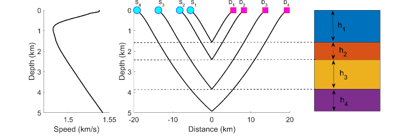
Figure 2: Acoustic sound traces. In the left panel, we show the sound speed profile of the Philippine sea Hodges (2002). In the middle panel, we show the results of numerical simulations of sound traces with incident angle $\theta_{0}=80^{o}$ and, in the right panel, we show the seismic model used. The thickness of each layer of the model matches the position where the corresponding sound trace is reflected. For clarity, we only show the simulations involving only 4 sources (receptors).

We have applied the above formulation to solve a small scale underwater seismic inversion problem. Artificial data were generated by simulating sound traces in ocean. We have used the sound speed profile of the Philippine Sea, available to public Hodges (2002), as shown in Figure 2. From the simulation, we obtained the travel times between the sources and detectors. The seismic inversion model was constructed using 46 layers while the real variables were digitalized with $R=3$ bits. This model yields 138 binary variables, for the present type of problem, it is the maximum number of variables that we can embed in the working graph of the D-Wave Advantage system available in Amazon.

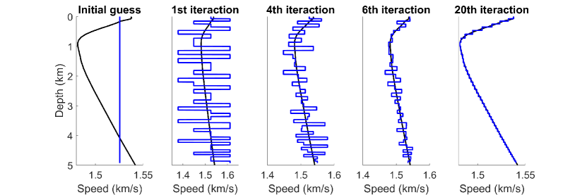
Figure 3: Seismic inversion obtained in the quantum annealer for different iterations. The black curve is the original sound speed profile and the blue curve is the result of the inversion obtained in the quantum annealer.

To perform the seismic inversion we have considered that all layers in the model match the position where the sound wave is reflected, as shown in Figure 2. The solution is presented in Figure 3, as can be seen, good results are obtained with 20 iteractions. We have also performed the inversion with a classical computer running the forward substitution algorithm to invert the lower triangular matrix in equation (8). When classical and quantum inversions are compared, we found that the relative error between them was $\approx 10^{-4}$, as shown in figure 3. This result shows that the quantum computer using the recursive approach to solve a system of linear equations has enough control to find solutions with good precision.

The results could also be compared to the benchmark provided by the condition number of the numerical problem at hand. When performing a numerical inversion procedure on the lower triangular matrix $\mathbf{M}$ to recover the solution $\mathbf{s}$ in Equation (8), a straightforward estimation of the lower bound of the relative error $\epsilon_{s}$ in $\mathbf{s}$ arising from the relative error $\epsilon_{t}$ in the righthand side vector $\mathbf{t}$ due to the numerical conditioning of $\mathbf{M}$ is given by Kincaid and Cheney (1991)

$$\epsilon_{s}=\kappa_{\infty}\epsilon_{t},$$ (16)

where $\kappa_{\infty}$ is the condition number given by

$$\kappa_{\infty}\geq\frac{\max_{j}(h_{j}/\cos\theta_{j})}{\min_{j}(h_{j}/\cos\theta_{j})}.$$ (17)

Therefore, the condition number relates the error associated with $\mathbf{t}$, $\epsilon_{s}$, and the error of the solution $\mathbf{s}$, $\epsilon_{s}$. In this particular application of seismic inversion, where distances are generally in the scale of $10^{3}m$, it is reasonable to assume that the figures are accurate up to the order of $\approx 10m$, with the next order of magnitude ($1m$) giving the scale of the error $\epsilon_{t}$. Given that the error $\epsilon_{t}$ can be estimated as $\approx 10^{-3}$ and the condition number is $\kappa_{\infty}\approx 1$, then we can estimate $\epsilon_{s}\approx 10^{-3}$ from (16 ). This shows that the error of the quantum approach comes from the inversion problem by itself and is of the same order as the classical approach.

VI Conclusions

Quantum computing represents a fundamentally different paradigm, an entirely different way to perform calculations. The Geoscience field and related industries are strong candidates to benefit from it. However, the performance of Geoscience inversion problems on current available quantum computers has so far been largely unexploited.

In this paper, we have solved a seismic inversions in a D-Wave quantum annealer. The seismic problem was written as a system of linear equations and then translated into a QUBO formulation. The results presented here indicate that the current available quantum annealers can solve a seismic inversion at a relatively small size with nearly the same accuracy as a classical computer. The proof-of-principle computations performed here show some promise for the use of quantum annealing in Geosciences.

The practical use of quantum annealing in Geosciences will require the ability to solve large problems. To address this issue, decomposer tools have been proposed to divide a large problem into small subproblems which can be solved individually by the quantum hardware Inc (2021b); Okada et al. (2019); Nishimura et al. (2019). Using such approach, it is possible to solve a large-sized problem using just a limited number of available qubits. Another interesting approach is the reverse annealing. Within this method, one starts from known local solutions which can be obtained in a classical computer. The annealing is performed backward from the known classical state to a state of quantum superposition, then proceeding forward it is possible to reach a new classical state that is a better solution than the initial one. Recently, it has been shown that it is possible to refine local solutions with recursive applications of reverse annealing Passarelli et al. (2020); Yamashiro et al. (2019); Venturelli and Kondratyev (2019); Arai et al. (2021). We believe that the development of hybrid quantum-classical methods, such as mentioned above, will be essential to solve complex seismic problems on quantum annealers in the near future.

Finally, we should mention that the problem solved here is well-conditioned, however, often Geoscience problems are ill-conditioned. An interesting question is whether quantum computers can solve ill-conditioned problems efficiently. In reference Clader et al. (2013), it was theoretically proposed that preconditioning methods can expand the number of linear systems problems that can achieve exponential speedup over classical computers. In future works, we plan to study the performance of the quantum annealers to solve ill-conditioned problems. Another attractive prospect for future work is the implementation of Geoscience problems in gate model computers, based either on superconducting or trapped ions technologies.

Conflict of Interest Statement

The authors declare that the research was conducted in the absence of any commercial or financial relationships that could be construed as a potential conflict of interest.

Author Contributions

A. M. Souza ran the quantum computer, analyzed the results, co-wrote, and reviewed the manuscript. E. O. Martins initiated the study, co-wrote, and reviewed the manuscript. N. Sá, I. Roditi , R. Sarthour and I. S. Oliveira co-wrote and reviewed the manuscript.

Funding

This work was supported by the Brazilian National Institute of Science and Technology for Quantum Information (INCT-IQ) Grant No. 465469/2014-0, the Coordenação de Aperfeiçoamento de Pessoal de Nível Superior - Brasil (CAPES) - Finance Code 001, Conselho Nacional de Desenvolvimento Científico e Tecnológico (CNPq) and PETROBRAS: Projects 2017/00486-1, 2018/00233-9 and 2019/00062-2. A. M. S. acknowledges support from FAPERJ (Grant No. 203.166/2017). I.S.O acknowledges FAPERJ (Grant No. 202.518/2019).

Supplemental Data

Data Availability Statement

Figure captions

1:function Solve($\mathbf{M}$, $\mathbf{t}$, $\mathbf{s_{0}}$, L, $N_{\mathrm{max}}$,$\epsilon$)

2:     $\mathbf{I}\leftarrow[1;1;1;\cdots;1]$

3:     for $c\leftarrow 1$ to $N_{\mathrm{max}}$ do

4:         $\mathbf{b}\leftarrow(\mathbf{t}+L\mathbf{MI}-\mathbf{Ms_{0}})/L$

5:         Construct the vetor $\mathbf{q}$ and the Matrix $\mathbf{A}$

6:         Convert $||\mathbf{A}\mathbf{q}-\mathbf{b}||^{2}$ to QUBO $\mathbf{q}^{\mathsf{T}}\mathbf{Qq}$

7:         Calculate $\mathbf{q^{*}}$

8:         From $\mathbf{q^{*}}$ recover $\mathbf{x}$

9:         $\mathbf{s}\leftarrow\mathbf{s_{0}}+L\mathbf{(x-I)}$

10:         if $||\mathbf{s}-\mathbf{s_{0}}||^{2}\leq\epsilon$ then

11:              Stop Loop

12:         else

13:              $\mathbf{s_{0}}\leftarrow\mathbf{s}$

14:              $L\leftarrow L/2$

15:         end if

16:     end for

17:     return $\mathbf{s}$

18:end function

Algorithm 1 Function to solve the system of equations $\mathbf{Ms}=\mathbf{t}$. The vector $\mathbf{s_{0}}$ is the initial guess for $\mathbf{s}$, $\epsilon$ is the tolerance, $N_{max}$ is the maximum number of iterations, and $L$ defines the interval where we expect to find the solutions (see text).

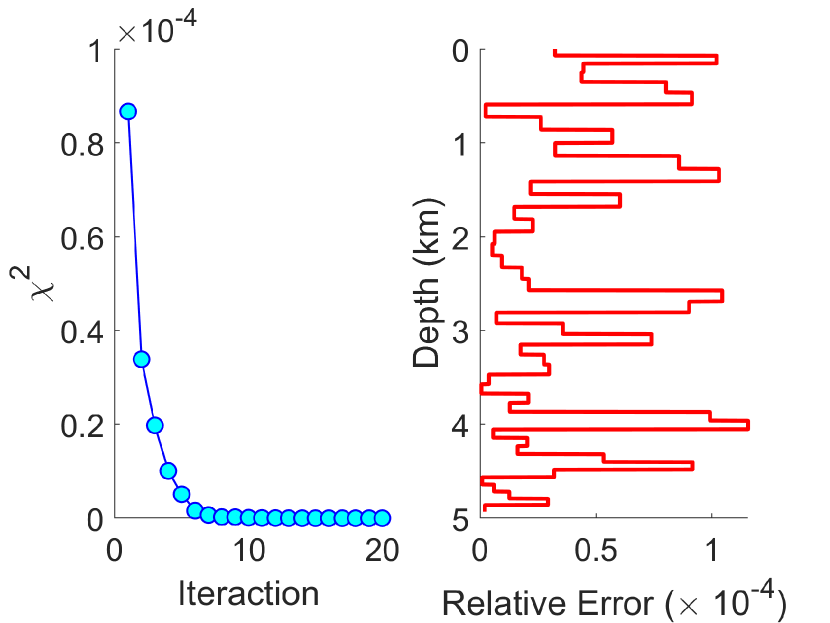
Figure 4: Comparisons between classical and quantum solutions. In the left panel, we show the $\chi^{2}$ test between the quantum annealing solution and the classical solution. The relative error between the classical and quantum solutions is shown as a function of the ocean depth in the right panel.

References

- Arute et al. (2019) Arute F, Arya K, Babbush R, Bacon D, et al JCB. Quantum supremacy using a programmable superconducting processor. Nature 574 (2019) 505–510. doi:https://doi.org/10.1038/s41586-019-1666-5.
- Zhong et al. (2020) Zhong HS, Wang H, Deng YH, Chen MC, et al LCP. Quantum computational advantage using photons. Science 370 (2020) 1460. doi:DOI:10.1126/science.abe8770.
- et. al. (2021) et al YW. Strong quantum computational advantage using a superconducting quantum processor. arXiv:2106.14734 (quant-ph) (2021).
- Kjaergaard et al. (2020) Kjaergaard M, Schwartz ME, Braumüller J, Krantz P, Wang JIJ, Gustavsson S, et al. Superconducting qubits: Current state of play. Annual Review of Condensed Matter Physics 11 (2020) 369.
- Bruzewicz et al. (2019) Bruzewicz CD, Chiaverini J, McConnell R, Sage JM. Trapped-ion quantum computing: Progress and challenges. PNAS 6 (2019) 021314.
- Job and Lidar (2018) Job J, Lidar D. Test driving 1000 qubits. Quantum Science and Technology 3 (2018) 030501. doi:https://doi.org/10.1088/2058-9565/aabd9b.
- Bourassa et al. (2021) Bourassa JE, Alexander RN, Vasmer M, Patil A, et al IT. Blueprint for a scalable photonic fault-tolerant quantum computer. Quantum 5 (2021) 392.
- Brod et al. (2019) Brod DJ, Galvao EF, Crespi A, Osellame R, Spagnolo N, Sciarrino F. Photonic implementation of boson sampling: a review. Advanced Photonics 1 (2019) 034001.
- Linke et al. (2017) Linke NM, Maslov D, Roetteler M, Debnath S, Figgatt C, Landsman KA, et al. Experimental comparison of two quantum computing architectures. PNAS 114 (2017) 3305.
- Devitt (2016) Devitt SJ. Performing quantum computing experiments in the cloud. Phys. Rev. A 94 (2016) 032329.
- O’Malley (2018) O’Malley D. An approach to quantum-computational hydrologic inverse analysis. Sci. Rep. 8 (2018) 6919. doi:https://doi.org/10.1038/s41598-018-25206-0.
- Golden and O’Malley (2021) Golden J, O’Malley D. Pre- and post-processing in quantum-computational hydrologic inverse. Quantum Information Processing 20 (2021) 176.
- Alulaiw and Sen (2015) Alulaiw B, Sen MK. Prestack seismic inversion by quantum annealing: Application to cana field. SEG Technical Program Expanded Abstracts (2015) 3507. doi:https://doi.org/10.1190/segam2015-5831164.1.
- Wei et al. (2006) Wei C, Zhu PM, Wang JY. Quantum annealing inversion and implemantation. Chinese J. Geophys. 49 (2006) 499.
- Greer and Malley (2020) Greer S, Malley O. An approach to seismic inversion with quantum annealing. SEG Technical Program Expanded Abstracts (2020) 2845. doi:https://doi.org/10.1190/segam2020-3424413.1.
- Nielsen and Chuang (2001) Nielsen MA, Chuang IL. Quantum computaion and quantum information (Cambridge University Press) (2001).
- Aaronson and Arkhipov (2011) Aaronson S, Arkhipov A. The computational complexity of linear optics. Proc. 43rd Annu. ACM Symp. Theory of Comput. (2011) 333.
- Farhi et al. (2001) Farhi E, Goldstone J, Gutmann S, Lapan J, Lundgren A, Preda D. A quantum adiabatic evolution algorithm applied to random instances of an np-complete problem. Science 292 (2001) 472.
- Albash and Lidar (2018a) Albash T, Lidar DA. Adiabatic quantum computation. Rev. Mod. Phys. 90 (2018a) 015002. doi:http://doi.org/10.1103/RevModPhys.90.015002.
- Aharonov et al. (2007) Aharonov D, van Dam W, Kempe J, Landau Z, Lloyd S, Regev O. Adiabatic quantum computation is equivalent to standard quantum computation. SIAM Journal of Computing 37 (2007) 166.
- Biamonte and Love (2008) Biamonte JD, Love PJ. Realizable hamiltonians for universal adiabatic quantum computers. Phys. Rev. A 78 (2008) 012352.
- Preskill (2018) Preskill J. Quantum computing in the nisq era and beyond. Quantum 2 (2018) 79. doi:https://doi.org/10.22331/q-2018-08-06-79.
- Barahona (1982) Barahona F. On the computational complexity of ising spin glass models. J. Phys. A: Math. Gen. 15 (1982) 3241–3253. doi:http://doi.org/10.1088/0305-4470/15/10/028.
- Ronnow et al. (2014) Ronnow T, Wang Z, Job J, Boixo S, Isakov S, Weckek D, et al. Defining and detecting quantum speedup. Science 345 (2014) 420.
- Mandra et al. (2016) Mandra S, Zhu Z, Wang W, Perdomo-Ortiz A, Katzgraber H. Strengths and weaknesses of weak-strong cluster problems: A detailed overview of state-of-the-art classical heuristics versus quantum approaches. Phys. Rev. A 94 (2016) 022337.
- Katzgraber et al. (2015) Katzgraber H, Hamze F, Zhu Z, Ochoa A, Munoz-Bauza H. Seeking quantum speedup through spin glasses: The good, the bad, and the ugly. Phys. Rev. X 5 (2015) 031026.
- Albash and Lidar (2018b) Albash T, Lidar DA. Demonstration of a scaling advantage for a quantum annealer over simulated annealing. Phys. Rev. X 8 (2018b) 031016.
- Denchev et al. (2016) Denchev V, Boixo S, Isakov S, Ding N, Babbush R, Smelyanskiy V, et al. What is the computational value of finite-range tunneling ? Phys. Rev. X 6 (2016) 031015.
- Li et al. (2018) Li RY, DiFelice R, Rohs R, Lidar DA. Quantum annealing versus classical machine learning applied to a simplified computational biology problem. npj Quantum Inf 4 (2018) 14. doi:https://doi.org/10.1038/s41534-018-0060-8.
- Baldassi and Zecchina (2018) Baldassi C, Zecchina R. Efficiency of quantum vs. classical annealing in nonconvex learning problems. PNAS 115 (2018) 1457.
- Hen et al. (2015) Hen I, Job J, Albash T, Ronnow T, Troyer M, Lidar D. Probing for quantum speedup in spin-glass problems with planted solutions. Phys. Rev. A 95 (2015) 042325.
- Brady and van Dam (2016) Brady LT, van Dam W. Quantum monte carlo simulations of tunneling in quantum adiabatic optimization. Phys. Rev. A 93 (2016) 032304.
- Crosson and Harrow (2016) Crosson E, Harrow AW. Simulated quantum annealing can be exponentially faster than classical simulated annealing. Proc. of FOCS (2016) 714.
- Jiang et al. (2017) Jiang Z, Smelyanskiy VN, Isakov SV, Boixo S, Mazzola G, Troyer M, et al. Scaling analysis and instantons for thermally-assisted tunneling and quantum monte carlo simulations. Phys. Rev. A 95 (2017) 012322.
- Lucas (2014) Lucas A. Ising formulations of many np problems. Front. Phys. 2 (2014) 5. doi:https://doi.org/10.3389/fphy.2014.00005.
- Li et al. (2021) Li R, Gujja S, Bajaj S, Gamel O, Cilfone N, Gulcher J, et al. Quantum processor-inspired machine learning in the biomedical sciences. Patterns 2 (2021) 100246. doi:https://doi.org/10.1016/j.patter.2021.100246.
- Neukart et al. (2017) Neukart F, Compostella G, Seidel C, von Dollen D, Yarkoni S, Parney B. Traffic flow optimization using a quantum annealer. Frontiers in ICT 4 (2017) 29. doi:10.3389/fict.2017.00029.
- Kitai et al. (2020) Kitai K, Guo J, Ju S, Tanaka S, Tsuda K, Shiomi J, et al. Designing metamaterials with quantum annealing and factorization machines. Phys. Rev. Research 2 (2020) 013319. doi:https://doi.org/10.1103/PhysRevResearch.2.013319.
- Mott et al. (2017) Mott A, Job J, Vlimant JR, Lidar D, Spiropulu M. Solving a higgs optimization problem with quantum annealing for machine learning. Nature 550 (2017) 375. doi:https://doi.org/10.1038/nature24047.
- Duan et al. (2020) Duan B, Yuan J, Yu CH, Huang J, Hsieh CY. A survay on hhl algorithm: From theory to applications in quantum machine learning. Phys. Lett. A 384 (2020) 126595.
- Dervovic et al. (2018) Dervovic D, Herbster M, Mountney P, Severini S, Usher N, Wossnig L. Quantum linear systems algorithms: a primer. arXiv:1802.08227v1 (2018).
- Harrow et al. (2009) Harrow AW, Hassidim A, Lloyd S. Quantum algorithm for linear systems of equations. Phys. Rev. Lett 103 (2009) 150502. doi:http://doi.org/10.1103/PhysRevLett.103.150502.
- Aaronson (2015) Aaronson S. Read the fine print. Nat. Phys. 11 (2015) 291–293. doi:https://doi.org/10.1038/nphys3272.
- Ambainis (2012) Ambainis A. Variable time amplitude amplification and quantum algorithms for linear algebra problems. Dürr C, Wilke T, editors, 29th International Symposium on Theoretical Aspects of Computer Science (STACS 2012) (Dagstuhl, Germany: Schloss Dagstuhl–Leibniz-Zentrum fuer Informatik) (2012), Leibniz International Proceedings in Informatics (LIPIcs), vol. 14, 636–647. doi:10.4230/LIPIcs.STACS.2012.636.
- Childs et al. (2017) Childs AM, Kothari R, Somma RD. Quantum algorithm for systems of linear equations with exponentially improved dependence on precision. SIAM J. Comput. 46 (2017) 1920–1950. doi:https://doi.org/10.1137/16M1087072.
- Wossing et al. (2018) Wossing L, Zhao Z, Prakash A. Quantum linear system algorithm for dense matrices. Phys. Rev. Lett 120 (2018) 050502. doi:https://doi.org/10.1103/PhysRevLett.120.050502.
- Shao and Xiang (2020) Shao C, Xiang H. Row and column iteration methods to solve linear systems on a quantum computer. Phys. Rev. A 101 (2020) 022322.
- Subasi et al. (2019) Subasi Y, Somma RD, Orsucci D. Quantum algorithms for systems of linear equations inspired by adiabatic quantum computing. Phys. Rev. Lett. 122 (2019) 060404.
- Rogers and Singleton (2020) Rogers ML, Singleton RL. Floating-point calculations on a quantum annealer: Division and matrix inversion. Front. Phys. 265 (2020) 8. doi:doi:10.3389/fphy.2020.00265.
- Borle and Lomonaco (2019) Borle A, Lomonaco SJ. Analyzing the quantum annealing approach for solving linear least squares problemss. Das GK, Mandal PS, Mukhopadhyaya K, Nakano S, editors, WALCOM: Algorithms and Computation (Springer) (2019), 289–301. doi:https://doi.org/10.1007/978-3-030-10564-8˙23.
- O’Malley and Vesselinov (2016) O’Malley D, Vesselinov VV. Toq.jl: A high-level programming language for d-wave machines based on julia. IEEE Conference on High Performance Extreme Computing (HPEC) (2016). doi:https://doi.org/10.1109/HPEC.2016.7761616.
- Chang et al. (2019) Chang CC, Gambhir A, Humble TS, Sota S. Quantum annealing for systems of polynomial equations. Sci. Rep. 9 (2019) 10258.
- Kearey et al. (2002) Kearey P, Brooks M, Hill I. An Introduction to Geophysical Exploration (Wiley), 3 edn. (2002).
- Bunyk et al. (2014) Bunyk PI, Hoskinson EM, Johnson MW, Tolkacheva E, Altomare F, Berkley AJ, et al. Architectural considerations in the design of a superconducting quantum annealing processor. IEEE Trans. Appl. Supercond. 24 (2014) 1700110. doi:https://doi.org/10.1109/TASC.2014.2318294.
- Dattani et al. (2019) Dattani N, Szalay S, Chancellor N. Pegasus: The second connectivity graph for large-scale quantum annealing hardware. arXiv:1901.07636 (quant-ph) (2019).
- Cai et al. (2014) Cai J, Macready B, Roy A. A practical heuristic for finding graph minors. ArXiv:1406.2741 [quant-ph] (2014).
- Pearson et al. (2019) Pearson A, Mishra A, Hen I, Lidar DA. Analog errors in quantum annealing: doom and hope. npj Quantum Information volume 5 (2019) 2347. doi:https://doi.org/10.1038/s41534-019-0210-7.
- Inc (2021a) [Dataset] Inc DWS. Qpu solver datasheet. file:///C:/Users/alexa/Downloads/09-1109B-C_QPU_Solver_Datasheet.pdf (2021a). Accessed: 2021-10-15.
- Pelofske et al. (2019) Pelofske E, Hahn G, Djidjev H. Optimizing the spin reversal transform on the d-wave 2000q. 2019 IEEE International Conference on Rebooting Computing (ICRC) (2019), 1–8. doi:10.1109/ICRC.2019.8914719.
- Hodges (2002) Hodges RP. Underwater Acoustics (Wiley) (2002).
- Kincaid and Cheney (1991) Kincaid D, Cheney W. Numerical Analysis: Mathematics of Scientific Computing (USA: Brooks/Cole Publishing Co.) (1991).
- Inc (2021b) [Dataset] Inc DWS. qbsolv documentation. https://docs.ocean.dwavesys.com/_/downloads/qbsolv/en/latest/pdf/ (2021b). Accessed: 2021-10-15.
- Okada et al. (2019) Okada S, Ohzeki M, MTerabe, Taguchi S. Improving solutions by embedding larger subproblems in a d-wave quantum annealer. Sci. Rep. 9 (2019) 2098.
- Nishimura et al. (2019) Nishimura N, Tanahashi K, Suganuma K, Miyama MJ, Ohzeki M. Item listing optimization for e-commerce websites based on diversity. Front. Comput. Sci. 1 (2019) 2. doi:https://doi.org/10.3389/fcomp.2019.00002.
- Passarelli et al. (2020) Passarelli G, Yip KW, Lidar DA, Nishimori H, Lucignano P. Reverse quantum annealing of the p-spin model with relaxation. Phys. Rev. A 101 (2020) 022331.
- Yamashiro et al. (2019) Yamashiro Y, Ohkuwaa M, Nishimori H, Lidar DA. Dynamics of reverse annealing for the fully connected p-spin model. Phys. Rev. A 100 (2019) 052331.
- Venturelli and Kondratyev (2019) Venturelli D, Kondratyev A. Reverse quantum annealing approach to portfolio optimization problems. Quantum Machine Intelligence 1 (2019) 17.
- Arai et al. (2021) Arai S, Ohzeki M, Tanaka K. Mean field analysis of reverse annealing for code-division multiple-access multiuser detection. Phys. Rev. Research 3 (2021) 033006.
- Clader et al. (2013) Clader BD, Jacobs BC, Sprouse CR. Preconditioned quantum linear system algorithm. Phys. Rev. Lett. 110 (2013) 250504.