Inverse Cosmography: testing the effectiveness of cosmographic polynomials using machine learning

Abstract

Cosmography has been referred to as a solution to the inverse scattering problem, which is reasonable since it allows us to calculate cosmological bounds from data samples by performing an expansion of the cosmological observables around the present time. Nevertheless, this approach is not properly an inverse scattering solution since the method only circumvents the problem to fit the equation of state (EoS) parameters (model-dependent) by replacing it with their fit of its cosmographic parameters (with a polynomial series-dependence). Therefore, the question that we want to answer is: can we construct a new cosmography approach where the cosmodynamical parameters can be fitted and then employ them to analyse the kinematics via its generic cosmographic parameters? By all means, without experimenting with the traditional problem of truncation of the series that all cosmography proposals in the literature argue. In this work, we present a solution to this question. A generic EoS depending solely on the form of $f_{i}(z)$ and its derivative is found, where this function can be any polynomial (mimicking a dark energy-like term) that allow the dynamics of a specific cosmological density. We test our generic EoS with standard cosmological models and with polynomials proposals as Padé and Chebyshev approximants. All of them reproduce $\Lambda$CDM at $z>1$ between 1-$\sigma$, but fail at lower observational redshift range. Interesting enough, a Padé (2,2) approximant has been considered inside a $f(z)$CDM-like model showing a transition in $z=1$. Also, we found that this is not assured since models with these characteristics have degeneracy and truncation problems that have a divergence at this redshift limit. With a Chebyshev (2,1) approximant, here proposed, the divergence is not present for large redshifts. To explore our results, also we present a new supernovae sample trained via a deep learning tool called Recurrent-Bayesian (RNN+BNN) network that can solve problems as overfitting at lower redshifts and increase the density of data points in this region, which can help to discern between cosmographies at 2-$\sigma$ of precision.

1 Introduction

To understand the cosmic accelerating evolution in a standard manner we often base our description of the Universe in a model-dependent way. This argument leads to a biased cosmic reconstruction of the dynamics of the universe, where the cosmological parameters suffer from degeneracies problems or cannot be well-tested with a good-fit convergence using observational samples. Currently, these problems fall into the window of cosmological tension parameter discussions, like those of $\sigma_{8}$ and $H_{0}$ [1]. Strategies towards a model-independent analysis to relax these problems require the assumptions of homogeneity and isotropy in a scenario where the cosmic dynamics is independent of the energy densities. On this line of thought, the so-called cosmography approach has been proved to be an optimized method that can reconstruct the dynamical evolution of the cosmic acceleration (via a dark energy-like term) without assuming a specific cosmological model (see [3, 2], and references therein).

For several years, Cosmography has been referred to as an inverse scattering approach, which is reasonable since it allows us to calculate cosmological constraints directly from the observational surveys by performing an expansion of the cosmological observables of interest around the present time ($a_{(z=0)}=a_{0}$). Nevertheless, Cosmography is not a proper inverse scattering approach since the method only circumvents the problem to fit the equation of state (EoS) parameters (with a model-dependency) by replacing it with their fit of its cosmographic parameters (with a polynomial series-dependence). Therefore, the question that we want to solve is: can we construct a new cosmography approach where the cosmological parameters are fitted as usual and then employ them to analyse the kinematics via its cosmographic parameters? Moreover, can this be done without experimenting with the traditional problem of truncation of the series.

An interesting work that tackles a similar question was addressed in [4], where a straightforward cosmography approach over the EoS was improved to test cosmological parametric versions of the dynamics of dark energy. In this approach, a homogeneous supernovae observational sample was used to perform the statistical analysis of specific dark energy parameterisations to obtain directly the kinematics of the cosmographic parameters. The conclusion of this proposal lies in the fact that is possible to set constraints over the cosmographic parameter values using the cosmostatistics analyses of the dynamics imposed in the dark energy-like term. Also, the idea of using supernovae data was to avoid biased results in relation with the Planck cosmic microwave background (CMB) temperature data, since this survey is best fitted with a $\Lambda$CDM model that is in mild tension with constraints from dynamical data probes. Some cosmography proposals available in the literature perform a test with this latter sample, which is misleading to consider since this approach is unlikely to reveal any new physics beyond an improved $\Lambda$CDM with higher corrections. And these corrections are directly linked to low redshift data precision –also in the context of a Bayesian approach–.

According to the above issues and with the results in [4], our proposal in this paper consists of an inverse technique that can obtain a generic equation of state without assuming directly a cosmographic series. Therefore, we relax two inherent cosmography problems, namely

1. The study of the dark energy dynamics (without a cosmological constant $\Lambda$) by proposing standard Taylor series or suitable Padé or Chebyshev polynomials evolving with a cold dark matter (CDM) fluid.

2. The calculations of the cosmographic parameters using (i) without truncation problems over the series/polynomials proposed.

As an extension of this approach, and in order to work with a homogeneous data sample at low redshift, in [5] a novel computational tool based in machine learning (ML) for supernovae, called Recurrent-Bayesian Neural Networks (RNN+BNN), was proposed. A deep learning architecture can develop a trained homogeneous supernovae sample in where the resulting dynamics of dark energy could lead to the necessity of another cosmological model different from $\Lambda$CDM. In such a scenario, our inverse cosmography approach can fit statistically very well since it is not necessary to consider higher-order corrections of the cosmography series to obtain a convergence best fit in comparison to the standard dark energy EoSs. Using trained data from a deep learning architecture for a homogeneous sample as supernovae show, from a Bayesian point of view, better evidence without dealing with the degeneracy of the models at the third order of the series. This aspect usually appears when a combination of surveys is considered [6]. This evidence $\mathcal{E}=\int{\mathcal{L}(\theta)P(\theta)d\theta}$, where $\theta$ of the vector of free cosmographic parameters, $P(\theta)$ is the prior distribution of these parameters and $\mathcal{L}$ if the maximum likelihood of the model under consideration, has been computed using a MultiNest method for different activation function (see Table 6 in [5]).

While in the near future, high-redshift spectroscopy surveys [7, 8, 9] or Gravitational Waves surveys [10, 11] will provide accurate data in redshifts of $2<z<5$, our present deep learning result [5] allows to acquire more density of precise data of one species, the modulus distance, in redshifts range $0.01<z<4$.

To achieve our goal, this paper is organised as follows: in Sec.2 we describe the standard background cosmography in order to get the inverse cosmography. In Sec.3 we present three standard cases for the EoS with dark energy-like terms $f(z)$ as cosmological fluids. Also, we introduce the description of the $f(z)$CDM model using Padé and Chebyshev polynomial approaches. We calculate the EoS derived from the inverse cosmography and their cosmographic parameters at present time up to the fourth order in the series. In Sec.4 we introduce the RNN+BNN architecture to train the supernovae Pantheon sample [5]. The recipe to perform this training is also explained. In Sec.5 we perform statistical analyses for the models considered and we show the information criteria results that allow us to carry out model selection. In Sec.6 we will discuss the main results. To make the treatment comprehensive, in the Appendix we present the exact expressions for the cosmographic parameters for each model under consideration.

2 Inverse cosmography

We start by describing the standard cosmography equations. As will follow, this approach considers a Taylor-like expansion of the scale factor around $z=0$, which is the only parameter that can measure the Hubble flow according to the cosmological principle, therefore we can write

$$a(t)=1+\sum_{n=1}^{\infty}\dfrac{1}{n!}\dfrac{d^{n}a}{dt^{n}}\bigg{|}_{t=t_{0}}(t-t_{0})^{n}\ ,$$ (2.1)

where the Hubble, deceleration, jerk and snap parameters give information of the late universe and are defined respectively as:

$$H(t)\equiv\dfrac{1}{a}\dfrac{da}{dt}\ ,\hskip 14.22636ptq(t)\equiv-\dfrac{1}{aH^{2}}\dfrac{d^{2}a}{dt^{2}}\ ,\hskip 14.22636ptj(t)\equiv\dfrac{1}{aH^{3}}\dfrac{d^{3}a}{dt^{3}},\ \hskip 14.22636pts(t)\equiv\dfrac{1}{aH^{4}}\dfrac{d^{4}a}{dt^{4}}\ .$$ (2.2)

Extra cosmographic parameters have longer definitions which involve higher order derivatives of $H(z)$ in a sequence given by: $\dot{a}=aH,\quad\ddot{a}=-qaH^{2},\quad\dddot{a}=jaH^{3},\quad d^{4}a/dt^{4}=saH^{4},\quad\text{and}\quad d^{5}a/dt^{5}=laH^{5}$.

The signs of each cosmographic parameter gives information about the cosmic kinetic scenario: the sign of the deceleration parameter $q$ indicates whether the universe is accelerating (negative sign) or decelerating (positive sign), the sign of $j$ determines the change of the universe dynamics and the value of $s$ is necessary to discriminate between evolving dark energy or $\Lambda$. From here we notice that divergences in Taylor series are observed at $z>1$, since the expansion is performed around $z=0$, as a consequence of the convergence radius. These cosmographic parameters are essential since their character over the sign immediately shows the kinematics of the universe. Moreover, all of them are not observable quantities, therefore we require to perform a data fit over a specific model rewritten in terms of these parameters using astrophysical observations.

At this point, we can relax the degeneracy problem among cosmological models –certainly, with the Cosmological Principle as the backbone of this approach–, and in some manner, the hypothesis model(s) under testing will be the best one(s) once we perform the corresponding statistical cosmology over it(them). The consequence of using this approach is the high degeneracy and divergence on the terms related to the cosmographic parameters. The current arguments to defend this method remain in the idea of more data, better precision and the divergence of the series can be alleviated per se. Even with these ideas, cosmography remains unsuitable if we continue to study it with the following methodology:

1. Propose a Taylor (polynomial) series for the Hubble parameter around the present time.

2. Write the luminosity distance as a function of the redshift.

3. Confront the cosmographic parameters in the series with the current astrophysical samples.

4. Set the bounds on the cosmographic parameters with several kinds of surveys.

The final task of this methodology remains in confronting the point that the kinematics of the universe can be understood by setting limits on the standard cosmography using not only Taylor series [13], but also Padé and Chebyshev polynomials to parameterise cosmic distances. The use of these polynomials eliminates the convergence problem at higher redshifts and therefore, the systematic errors due the truncated Taylor series [14, 15]. More interesting approaches have been done towards a cosmography equation of state [16] or to link the late universe expansion with the early universe via a parametric cosmography [17]. However, none of them have yet set a non-stop-rule on the proposed cosmographic series with the use of combined observational samples. Over the general ideas up to now, a low order of the series expansion will generate values within the error propagation of the cosmographic parameters, while a high order of the propagation can be possible by using a larger sample that includes data points at higher redshift. This transition of redshift regions can be treated by considering different data samples. In the end, the amount by which the series will be well truncated depends on the quality of the measurements, and even then, systematic characteristics in the observational data continue to give the wrong results.

All these proposals express concern about finding not only a model-independent scenario but the endless loop tests of different kinds of polynomials in order to found a well-fitted description of the kinematics of the universe. In this direction, in [4] a mathematical expression to obtain the EoS for a specific dynamical model was proposed. This expression allows us to obtain the cosmographic parameters without assuming directly a cosmography-dependent polynomial series over them. Along the rest of this paper, we are going to refer to this approach as inverse cosmography.

With the inverse cosmography approach, we can obtain directly the cosmographic parameter values by fitting a specific function that can replace the standard dark energy-like term without dealing with the mentioned problems, i.e. we can constrain directly the cosmological parameters for the model and use them to compute the cosmographic parameters, e.g $q(z)$ and $j(z)$ (also $q_{0}$ and $j_{0}$) without considering higher corrections over them [15] or perform a change of variables over the redshift to avoid divergences.

To derive the inverse cosmography, we start as usual: with the spatial flatness hypothesis on the Hubble function as

$$\left(\frac{H(z)}{H_{0}}\right)^{2}=\Omega_{k}(1+z)^{2}+\Omega_{m}(1+z)^{3}+\Omega_{r}(1+z)^{4}+\Omega_{i}f_{i}(z),$$ (2.3)

where curvature $\Omega_{k}$ and radiation $\Omega_{r}$ contributions can be neglected in a late universe scenario, and the density closure relation is that $\Omega_{m}+\Omega_{i}=1$. The term $\Omega_{i}$ is related to the standard description of the current universe dynamics once the form of $f(z)$ is given. From here we are going to refer to $i=\Lambda$ as standard dark energy scenarios and $i=p$ as polynomial scenarios with their Hubble flow function given by, respectively

$$\left(\frac{H(z)}{H_{0}}\right)^{2} = \Omega_{m}(1+z)^{3}+\Omega_{\Lambda}f_{\Lambda}(z),$$ (2.4)

$$\left(\frac{H(z)}{H_{0}}\right)^{2} = \Omega_{m}(1+z)^{3}+\Omega_{p}f_{p}(z),$$ (2.5)

where $\Omega_{\Lambda}=1-\Omega_{m}$ and $\Omega_{p}$ is a CDM-fluid related to the polynomial case.

However, this approach requires a fiducial model, e.g. we can assume a flat quintessence model or a dynamical dark energy model. Therefore, we can write a generic expression for the cosmological EoS where we do not impose any form of dark energy-like $\Omega_{i}$ by formally solve (2.3) to obtain

$$w(z)=-1+\frac{1}{3}(1+z)\frac{f_{i}(z)^{\prime}}{f_{i}(z)},$$ (2.6)

where the prime denotes $d/dz$. Notice that this generic EoS depends solely on the form of $f_{i}(z)$. This is an interesting result since we obtain an EoS that only requires a functional form of $z$ and its derivative, e.g this function can be any polynomial at hand that allow the dynamics of a specific cosmological density.

Following the inverse cosmography idea, we can use the definitions (2.2) and (2.6) with the chain rule $\dot{}=d/dt=-(1+z)H(z)d/dz$, to obtain our new set of cosmographic parameters in terms $H(z)$ and its derivatives:

$$q(z)=-1+\frac{1}{2}(1+z)\frac{[H(z)^{2}]^{\prime}}{H(z)^{2}},$$ (2.7)

$$j(z)=\frac{1}{2}(1+z)^{2}\frac{[H(z)^{2}]^{\prime\prime}}{H(z)^{2}}-(1+z)\frac{[H(z)^{2}]^{\prime}}{H(z)^{2}}+1,$$ (2.8)

$$s(z)=-\frac{1}{6}(1+z)^{3}\frac{[H(z)^{2}]^{\prime\prime\prime}}{H(z)^{2}}+\frac{1}{2}(1+z)^{2}\frac{[H(z)^{2}]^{\prime\prime}}{H(z)^{2}}+(1+z)\frac{[H(z)^{2}]^{\prime}}{H(z)^{2}}-1.$$ (2.9)

By solving and evaluate them at $z=0$ we get the usual cosmographic series

$$H(z) = H_{0}+\frac{dH}{dz}\bigg{\rvert}_{z=0}z+\frac{1}{2!}\frac{d^{2}H}{dz^{2}}\bigg{\rvert}_{z=0}z^{2}+\frac{1}{3!}\frac{d^{3}H}{dz^{3}}\bigg{\rvert}_{z=0}z^{3}+\ldots$$ (2.10)

Similar expressions can be calculated by expressing everything in terms of the function normalised by the Hubble constant, $E(z)=H(z)/H_{0}$ and its derivatives. Nonetheless, the information we can obtain from this is exactly equivalent.

3 The models

In this work, we analyse three standard dark energy scenarios and two polynomial approaches to find directly their corresponding EoS using our generic equation (2.6). The first subsection is devoted to the standard $w$CDM model and Taylor-like parameterisations as Chevallier-Polarsky-Linder (CPL) and Redshift Squared (RS). In the second subsection the scenario presented will be a $f(z)$CDM-like approach based in Padé (2,2) and Chebyschev (2,1) polynomial expressions. To make the treatment comprehensive, in the following sections we present the cosmographic parameters for each model at the present time. In the Appendix, we develop the exact expressions for the general cosmographic parameters for each model under consideration.

3.1 Standard equations of state

As usual when we have to deal with a specific dark energy form with

$$f_{\Lambda}(z)=\text{exp}\left[3\int^{z}_{0}\frac{1+w_{\Lambda}(\tilde{z})}{1+\tilde{z}}d\tilde{z}\right],$$ (3.1)

we do not have a theoretical consensus on how to choose the best $w_{\Lambda}(z)$, and only an optimal form that can be cosmologically viable, e.g. for quintessence models ($w_{\Lambda}=\text{constant}$), we have $f_{\Lambda}(z)=(1+z)^{3(1+w_{\Lambda})}$. For a cosmological constant if $w_{\Lambda}=-1$ then $f_{\Lambda}=1$. Constrictions over the free parameters in the models are a useful way to compare the relative performance of several kinds of surveys to reconstruct the cosmic expansion [18]. Nonetheless, a generic form of $w_{\Lambda}$ remains unknown.

By using (2.7)-(2.8)-(2.9), we can easily derive the cosmographic parameters without dealing with higher derivatives for the solution of $H(z)$. Also, the cosmographic expressions obtained will show a relation between the kinematics and the dynamics of the universe. For this task, we are going to consider the following models:

3.1.1 $w$-constant flat cosmological case ($w$CDM)

This model can be modeled by:

$$\left(\frac{H(z)}{H_{0}}\right)^{2}=\Omega_{m}(1+z)^{3}+\Omega_{\Lambda}(1+z)^{3(1+w)},$$ (3.2)

where $\Omega_{m}$ is the present matter density and $\Omega_{\Lambda}=(1-\Omega_{m})$ the dark energy density. According to this model, and using our inverse cosmographic parameters defined above, we compute the following cosmographic parameters:

$$q(z)=\frac{1}{2}\left[\frac{3w\Omega_{m}}{\left(\Omega_{m}-1\right)(z+1)^{3w}-\Omega_{m}}+3w+1\right],$$ (3.3)

$$j(z)=\frac{[9w(w+1)+2]\left(\Omega_{m}-1\right)(z+1)^{3w}-2\Omega_{m}}{2\left(\Omega_{m}-1\right)(z+1)^{3w}-2\Omega_{m}},$$ (3.4)

$$s(z)=-\frac{[9w(w+1)+2]\left(\Omega_{m}-1\right)(w-z)(z+1)^{3w}+2z\Omega_{m}}{2(z+1)\left[\left(\Omega_{m}-1\right)(z+1)^{3w}-\Omega_{m}\right]},$$ (3.5)

where we notice that for dust $w=0$: $q=1/2$, $j=1$ and $s=0$ holds for any redshift. If we consider the evaluation of these parameters at $z=0$ and for a particular value of $w_{\Lambda}=-1$ we recover the standard $\Lambda$CDM scenario: $2q_{0}+j_{0}+s_{0}=2(\Omega_{m}-1)$.

3.1.2 Chevallier-Polarski-Linder (CPL) case

The evolution for this model [19, 20] can be represented by two parameters that exhibit the present value of the EoS $w_{0}$ and its overall time evolution $w_{a}$:

$$\left(\frac{H(z)}{H_{0}}\right)^{2} = \Omega_{m}(1+z)^{3}+\Omega_{\Lambda}(1+z)^{3(1+w_{0}+w_{a})}e^{-\left(\frac{3w_{a}z}{1+z}\right)}.$$ (3.6)

Following the above prescription, we can obtain the following cosmographic parameters at present time:

$$q_{0} = \frac{\left(3w_{0}+1\right)\left(\Omega_{m}-1\right)-\Omega_{m}}{2\left(\Omega_{m}-1\right)-2\Omega_{m}},$$ (3.7)

$$j_{0} = \frac{1}{2}\left[-\left(3w_{a}+2\right)\left(\Omega_{m}-1\right)-9w_{0}^{2}\left(\Omega_{m}-1\right)-9w_{0}\left(\Omega_{m}-1\right)+2\Omega_{m}\right],$$ (3.8)

$$s_{0} = \frac{\left[\left(-9w_{0}-2\right)w_{a}-w_{0}\left(9w_{0}\left(w_{0}+1\right)+2\right)\right]\left(\Omega_{m}-1\right)}{2\left(\Omega_{m}-1\right)-2\Omega_{m}}.$$ (3.9)

3.1.3 Redshift squared (RS) case

This model [21] can relax CPL parameterisation divergency at low redshift regions and can be well-behaved at $z\rightarrow-1$. The evolution of this model is given by

$$\left(\frac{H(z)}{H_{0}}\right)^{2} = \Omega_{m}(1+z)^{3}+(1-\Omega_{m})(1+z)^{3(1+w_{0})}(1+z^{2})^{\frac{3w_{a}}{2}}.$$ (3.10)

For this case the cosmographic parameters at present time are

$$q_{0} = \frac{1}{2}\left[3\left(\Omega_{m}-\left(w_{0}+1\right)\left(\Omega_{m}-1\right)\right)-2\right],$$ (3.11)

$$j_{0} = \frac{1}{2}\left[2-3\left(w_{a}+3w_{0}\left(w_{0}+1\right)\right)\left(\Omega_{m}-1\right)\right],$$ (3.12)

$$s_{0} = -\frac{1}{2}\left[\left(-9w_{0}-6\right)w_{a}-w_{0}\left(9w_{0}\left(w_{0}+1\right)+2\right)\right]\left(\Omega_{m}-1\right).$$ (3.13)

3.2 $f(z)$CDM Padé-like equations of state

The Padé approximant for cosmographic analyses [22] has been shown to have larger convergence radius in comparison to Taylor-like series, as the ones described above, and it is proving to be an optimal choice to extrapolate the analysis to higher redshifts as:

$$P_{(n,m)}(z)=\dfrac{\displaystyle{\sum_{i=0}^{n}a_{i}z^{i}}}{1+\displaystyle{\sum_{j=1}^{m}b_{j}z^{j}}}\,,$$ (3.15)

where the Padé approximant $P_{(n,m)}$ of order $n/m$, defines the ratio between two standard Taylor-like series as $f(z)=\sum_{i=0}^{\infty}a_{i}z^{i}$. In the latter reference, a possible extension to the analysis up to $z\sim 6$ for a Padé approximants of order (2,2) was presented. In our inverse cosmography approach we are going to consider this order for the polynomial since our deep learning training data is up to this redshift range. Following the proposal in [17], but taking into account the full definition for the Padé approximant, we write a new background evolution as

$$f_{p}(z)=\frac{P_{0}+P_{1}z+P_{2}z^{2}}{1+Q_{1}z+Q_{2}z^{2}},\quad\rightarrow\quad P_{(2,2)}=\frac{H(z)}{H_{0}}=\frac{1+P_{1}z+P_{2}z^{2}}{1+Q_{1}z+Q_{2}z^{2}},$$ (3.16)

where in the standard cosmography approach, each coefficient of the polynomial is a function that depends on the cosmographic parameters [6], making the analysis a loop problem because of the model-dependent on every of them.

At this point, we can apply our inverse cosmography approach over a $f(z)$CDM-like model, where $\Lambda$ is replaced by a Padé (2,2) polynomial in (2.5) and then obtain its characteristic EoS via (2.6)

$$w(z)_{\text{Pad\'{e}}}=-1+\frac{(z+1)\left[P_{1}\left(1-Q_{2}z^{2}\right)+P_{2}z\left(Q_{1}z+2\right)-P_{0}\left(2Q_{2}z+Q_{1}\right)\right]}{3\left[z\left(P_{2}z+P_{1}\right)+P_{0}\right)\left(z\left(Q_{2}z+Q_{1}\right)+1\right]},$$ (3.17)

from where if we consider $P_{0}=1$ we obtain the EoS for Padé (2,2). This term in the denominator will be important from a computational point of view, since will allow us to integrate without having divergencies at low redshift (see Sec.5.2). Notice how we recover $\Lambda$CDM at larger redshifts. According to this proposal and considering the Padé (2,2) (3.16) as $f_{p}(z)$ in (2.5), we can compute the corresponding cosmographic parameters at present time using again (2.7)-(2.8)-(2.9):

$$q_{0} = \frac{3\Omega_{m}+\Omega_{p}\left(-P_{1}-Q_{1}\right)}{2\left(\Omega_{m}+\Omega_{p}\right)}-1,$$ (3.18)

$$j_{0} = \frac{\Omega_{p}\left[P_{1}\left(Q_{1}+1\right)+P_{2}+Q_{1}\left(Q_{1}+1\right)-Q_{2}\right]}{\Omega_{m}+\Omega_{p}}+1,$$ (3.19)

$$s_{0} = 1-\frac{\Omega_{m}+\Omega_{p}\left[-\left(P_{1}+1\right)Q_{1}-P_{2}Q_{1}+Q_{1}\left[Q_{1}\left(-\left(P_{1}+Q_{1}\right)\right)-Q_{1}\right]+Q_{2}\left(P_{1}+2Q_{1}\right)+Q_{2}\right]}{\Omega_{m}+\Omega_{p}}$$ (3.20)

$$-\frac{\left(P_{1}+P_{2}\right)\Omega_{p}}{\Omega_{m}+\Omega_{p}}.$$

From these latter equations we see that for the case with $P_{i}=Q_{i}=0$, we recover a $\Lambda$CDM EoS and its respectively cosmographic parameters at present time $q_{0}=-1$, $j_{0}=1$, $s_{0}=0$. This is without calibrating the luminosity distance as it is usually done in standard cosmography.

3.3 $f(z)$CDM Chebyshev-like equations of state

In [15] was presented a method to optimize the standard technique of rational polynomials and consisted in defining the $(n,m)$ rational Chebyshev approximant with a coefficient $b_{0}\neq 0$ as

$$R_{(n,m)}(z)=\dfrac{\displaystyle{\sum_{i=0}^{n}}\ a_{i}T_{i}(z)}{1+\displaystyle{\sum_{j=1}^{m}}\ b_{j}T_{j}(z)}\ ,$$ (3.21)

was proposed. Applying a similar procedure used to obtain the Padé approximants, we can compute the background evolution with a rational Chebyshev $R_{(2,1)}$ as

$$f_{p}(z)=\frac{a_{0}+a_{1}z+2a_{2}z^{2}-a_{2}}{1+b_{1}z},\quad\rightarrow\quad R_{(2,1)}=\frac{H(z)}{H_{0}}=\frac{a_{3}+a_{1}z+2a_{2}z^{2}}{1+b_{1}z},$$ (3.22)

where $a_{3}=a_{0}-a_{2}$. Once again, in the standard cosmography approach, each coefficient $a_{i}$ and $b_{i}$ is a function that depends solely on the cosmographic parameters [15]. To relax the model-dependent loop problem, we calculate, as we did in the Padé case, our inverse cosmography approach as $f(z)$CDM-like model, where $\Lambda$ is replaced now by the rational Chebyshev $R_{(2,1)}$ in (2.5) and then obtain its characteristic EoS via (2.6)

$$w(z)_{\text{Chebyshev}}=-1+\frac{\left[2a_{2}z\left(b_{1}z+2\right)-a_{3}b_{1}+a_{1}\right](z+1)}{3\left(z\left(2a_{2}z+a_{1}\right)+a_{3}\right)\left(b_{1}z+1\right)},$$ (3.23)

from where $a_{3}=a_{1}/b_{1}$ to avoid any divergencies. We will perform a change of variable over $a_{0}$ once we integrate this EoS in Sec.5.2, in this manner we preserved the same expression for Chebyshev approximant (3.22). We recover again $\Lambda$CDM at larger redshifts. Now, we can compute the corresponding cosmographic parameters at present time using (2.7)-(2.8)-(2.9):

$$q_{0} = \frac{\left(a_{1}-a_{3}b_{1}\right)\Omega_{p}+3\Omega_{m}}{2\left(a_{3}\Omega_{p}+\Omega_{m}\right)}-1,$$ (3.24)

$$j_{0} = \frac{\left[a_{1}\left(-b_{1}-1\right)+a_{3}b_{1}\left(b_{1}+1\right)+2a_{2}+a_{3}\right]\Omega_{p}+\Omega_{m}}{a_{3}\Omega_{p}+\Omega_{m}},$$ (3.25)

$$s_{0} = \frac{\left[-a_{1}\left(b_{1}+1\right)+a_{3}b_{1}\left(b_{1}+1\right)+2a_{2}+a_{3}\right]\Omega_{p}+\Omega_{m}}{a_{3}\Omega_{p}+\Omega_{m}}.$$ (3.26)

At this point, in the cases with $a_{1}=a_{2}=a_{3}=0$ and $b_{1}=0$, we obtain a cosmology with a universe that is decelerating at the present time and with a preference for a cosmological constant. Noteworthy, this theoretical approach allows us to see that the cosmography is sensible to the values of the coefficient for this polynomial and present an anti-correlation between the cosmographic parameters. Notice that this result has been discussed in [17] after an exhaustive statistical analysis with data sets. We obtain the same result without considering cosmostatistics tools yet. We verify our arguments in Sec.5 and extend them with deep learning methods.

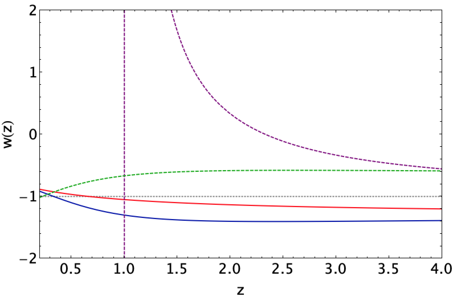
Figure 1: Equation of state for the standard cosmological models Sec.(3.1) and $f(z)$CDM cosmological models Secs.(3.2-3.3). For this evolution, the $\Lambda$CDM (grey dotted line), the standard models CPL and RS (red and blue solid lines, respectively) and the Padé (2,2) and Chebyshev (2,1) (purple and green dashed lines, respectively) are assumed with negative values of $w_{i}$, and positive values for all the free coefficients in the polynomials.

In Fig. 1, a comparison between our EoS is shown. According to the values considered for each of the free coefficients in the models, our analyses show a disagreement with [23] and [17] since the standard models behave as expected, the polynomial choices show a quintessence behaviour for $z>1$. Notice how both polynomials asymptotically approach each other near to $z\sim 4$ (our optimal redshift to perform the deep learning training, as we shall see below). Also, in the latter reference it was suggested that Padé (2,2) can be a good choice in redshift regions $z<1$, but from its EoS, we obtain that at $z=1$ there is a divergence. So the link between their toy model and the Padé approach is never reached. The reason for their results lies in the use of biased best fits that experiment truncation problems to test this toy model.

4 The method

To understand the inverse cosmography at high redshift, we require an observational sample in a redshift range where the kinematics can offer tight constraints over the cosmological parameters of the model. The computational method adopted in this paper allows us to further extend the cosmographic fit up to $z\approx 4$, with less than 2-$\sigma$ C.L. We can compare this analysis with studies where the use of Gamma Ray Burst (GRB) data can be employed up to $z\approx 6$. While exhibiting a strong correlation with their peak energy, the errors lead to biased results and the calibration at low-redshift is cosmology-dependent [24].

In Ref.[5], one of us proposed a novel deep learning architecture to extend the observational redshift range for late-time surveys, specifically for supernovae Type Ia. The results presented offer a way to study the evolution of dark energy models from an EoS point of view. Furthermore, a modified version of this algorithm can be employed to adapt our inverse cosmography and constrain the kinematics described by the polynomials at hand. For this method, we combine two architectures: the Recurrent Neural Networks (RNN) and the Bayesian Neural Networks (BNN). From this point forward, we will refer to this method as the RNN+BNN network. In the next sections we present our objective by describing the methodology to implement our inverse cosmography in this architecture. With this computational methodology, we can train a neural network with their confidence regions for specific homogeneous data. Additionally, RNN+BNN network minimizes the computational batch of expensive codes for dark energy models and probes the deviation from the $\Lambda$CDM scenario at large redshifts for a supernovae trained sample. In this section, we start by describing the supernovae sample used to train the network. Afterward, we present the main methodology for each RNN and BNN neural networks to implement these cosmographic models. Finally, we will describe the RNN+BNN architecture employed to implement the inverse cosmography. This method allows us to constrain at high redshifts ($z=4$) the inverse cosmographic parameters, which describes the kinematical state of the Universe without dealing with the convergence (or degeneracy) problems in the polynomials.

4.1 Supernovae sample

The most recent supernovae Type Ia sample is considered to be trained using the combination of the two networks described in the next two subsections. The so-called Pantheon supernovae sample consists of 40 bins [27] with 1048 SNIa compressed in a redshift range $[0.01,2.3]$. Type Ia supernovae can give determinations of the distance modulus $\mu$, whose theoretical prediction is related to the luminosity distance $d_{L}$. As we are considering spatial flatness, the $d_{L}$ is related to the comoving distance $D$ through $d_{L}(z)=c{H_{0}^{-1}}(1+z)D(z),$ where $c$ is the speed of light. From here we can compute the normalised Hubble function $H(z)/H_{0}$ by taking the inverse of the derivative of $D(z)$ with respect to $z$

$$D(z)=\int^{z}_{0}\frac{H_{0}}{H(\tilde{z})}d\tilde{z},$$ (4.1)

where $H_{0}$ is the Hubble constant prior value used to normalize the quantity $D(z)$.

4.2 Recurrent Neural Networks (RNN) for supernovae

To perform this first part of the neural network (NN), we consider a non-linear regression method using the supernovae sample described previously. The main idea consists in adopting a real target to train the NN for each data point. If the first data point trained is far away from the real data, then the algorithm penalizes this point and continues the process until it reaches a true value. Once the training is done for the entire sample, then the algorithm proceeds to minimise the loss function, this can be done using a Mean Squared Error (MSE) function combined with an Adam optimizer.

To set the architecture for this NN, we design a cell were the output data ($\mu(z)$) of the previous step is used to calculate the new one. Each cell is provided with the information of the output value using the following equations:

$$h^{<t>} = g(W_{h}\cdot h^{<t-1>}+W_{x}\cdot x^{<t>}+b_{a}),$$ (4.2)

$$y^{<t>} = g(W_{y}\cdot h^{<t>}+b_{y}),$$ (4.3)

where $b$ is the bias, $g$ is the activation function, $y^{<t>}$ is the output and $h^{<t>}$ and $h^{<t-1>}$, are the hidden state and its value before it, respectively. The $g$ function is given by $g=\tanh(x)$, in the range $(-1,1)$.

4.3 Bayesian Neural Networks (BNN) for supernovae

To solve the problem of overfitting in the networks, we perform the addition of posterior distributions making the networks probabilistic. First, we can compute the probability distribution over a specific weight given in the distribution of the trained data and insert this as a new input for the next distribution. Finally, an entire distribution can be obtained after $n$ steps, which will increase the prediction accuracy and confidence phase spaces. The prior distribution on the weight function for a new input point $x$ can be calculated by integrating the following equation:

$$p(\mathbf{y}^{*}|\mathbf{x}^{*},\mathbf{X},\mathbf{Y})=\int p(\mathbf{y}^{*}|\mathbf{x}^{*},\mathbf{\omega})p(\mathbf{\omega}|\mathbf{X},\mathbf{Y})\mathbf{d\omega},$$ (4.4)

where X and Y denotes the redshift $z$ and the modulus distance $\mu$, respectively. $p(\omega|X,Y)$ is the posterior distribution over the space of parameters. Furthermore, we can compute the model uncertainty applying this distribution in the training $n$-times.

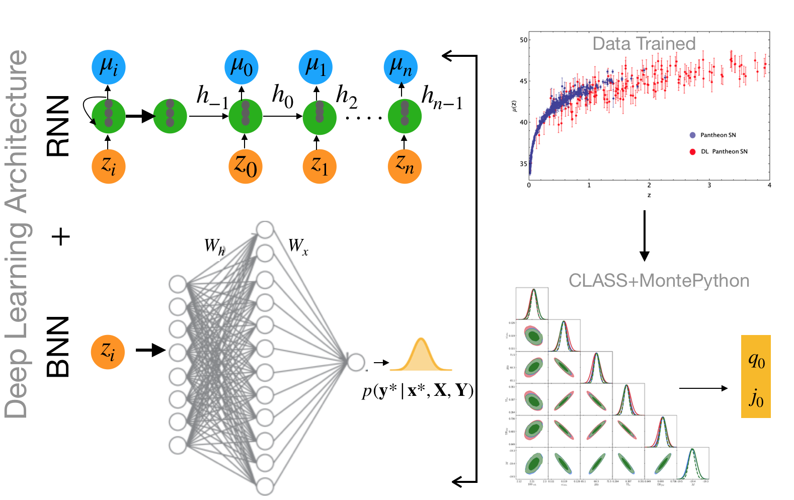
Figure 2: Left Top: Deep learning RNN architecture. The input $z_{i}$ are the redshifts and the output $\mu_{i}$ is the modulus luminosity distance. In this figure we consider only one layer and the grey colored circles inside each green color node represent the number of neurons $h_{i}$. The values for layers and neurons are given in Step 1, Sec. 4.4. Notice how each neuron receives inputs values from the latter neurons through each step $n$. In each step, an activation function Tanh is associated. Left Bottom: Deep learning BNN architecture. The network consists of one hidden layer with twelve nodes and an output layer with a single node. The weight functions between input a hidden layers are given in Eqs.(4.2). The result prior distribution is given by Eq.(4.4). Top Right: Supernovae final data sample trained using RNN+BNN. The RNN generates the data up to $z=4$ (see Figure 3). The BNN calculates the error bars at 1-$\sigma$ C.C for the training. Bottom Right: Bayesian process using CLASS + MontePython tools to compute the cosmographic parameters best fits and their evidence using the SN final data sample.

4.4 RNN+BNN network for inverse cosmography

To perform the deep learning training we follow the methodology given in [5]. The finals steps will detail the modifications performed to insert our inverse cosmographic models. We start by dividing the process into two blocks: first, by describing the deep learning process and the characteristic on the NN architecture. Secondly, the process to compute the best fit values for the cosmographic parameters.

• Training the supernovae data with RNN+BNN architecture

  • Step 1. Construction of the neural network (NN). For RNN we choose a Tanh activation function with 8 hyperparameters: Size=4, Epochs=100, Layers=1, Neurons=100, Bathsize=10. And a variational dropout composed of an input $z$, a hidden state $h$, and an output $\mu(z)$. A diagram of this architecture was developed in [5], also it demonstrated why a Tahn function is adequate to train supernovae data from a Bayesian point of view.

  • Step 2. Organising the supernovae data. We ordering the Pantheon data from higher to low redshift with a choice of a number of steps $n=4$. We ordered in this manner since a recurrent network feed itself during the training, e.g. one network with a neuron will have a connection from the input and also from the output of its previous time step, from which feed itself. Furthermore, this will have the advantage to have more information to train in regions where the density of data points is higher (at low redshifts for this SN sample) up to regions where there is a lower density of data points (at high redshifts for this SN sample).

  • Step 3. Calculation of the confidence errors via BNN. Given that the neural networks tend to overfit, it is important to choose a mode of regularisation. BNN allows our algorithm to calculate errors via a regularisation method. Our dropout has the following parameter: the probability to drop the input is $0$, this is because after testing several times, we found that our models could not be training with input dropout due to the loss of information. Since the cost function is MSE type (see Figure 3, bottom plot) we can use Adam optimizer.

  • Step 4. Results from the training. After the training, we read the model and apply $500$ times the same dropout to our initial model. The predicted sample with the above characteristics consist of 1810 data points in a redshift range of $[0.01-4.0]$. See Figure 3, top plot).

• Inverse Cosmography in Deep Learning RNN+BNN:

  • Step 5. Compute $\mu(z)$ for each cosmological model. We obtain $\mu$ by using the cosmological models described in Sec.3 and integrating them to obtain $H(z)/H_{0}$. At this step we increase the number of epochs up to 1000.

  • Step 6. Calculate the best fits cosmographic parameters. We modified the publicly version codes CLASS and Monte Python to constrain the models from Sec.3 using RNN+BNN Pantheon sample from the Step 4 obtained and add them in Step 5.

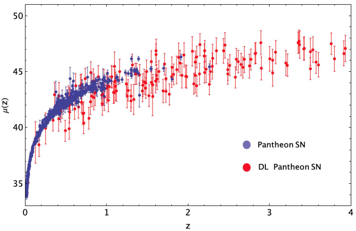
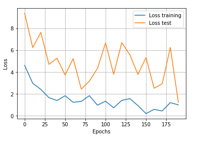
Figure 3: Top: Deep learning training for Pantheon sample up to $z=4$. The error bars represent the 1-$\sigma$ C.C. The Pantheon observational data is given by the purple dots and the training RNN+BNN supernovae data is given by the red points. Bottom: Loss versus epochs plot for the training RNN+BNN supernovae data. This training was performed using a Tanh as activation function, which shows a better Bayesian evidence according to [5].

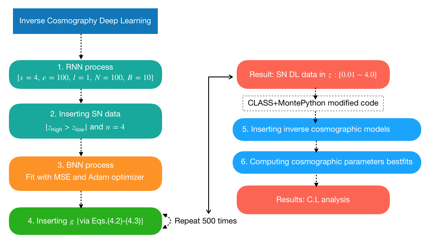
Figure 4: The algorithm tree performed to obtain the cosmographic parameters best fits via inverse cosmography using the DL supernovae data trained. The full steps are described in Sec. 4.4. The teal color box denotes the RNN architecture. The orange color box denotes the BNN architecture, related to the calculations of the errors. The green box denotes the inclusion of activation functions to train the observed data. Red boxes denote the final results in each tree. Blue boxes denote the process related to the standard MCMC and Bayesian calculations using CLASS+MontePython codes. Our modified version includes the models described in Eqs.(3.2)-(3.6)-(3.10)-(3.17)-(3.23).

We notice that this algorithm can easily perform the fit of cosmological models with independent model priors. The only restriction is the activation function, which can be viewed as a choice of a prior since it is relevant in regions where the training data is sparse or even non-existent and the resulting trained supernovae sample depends on this choice. Nevertheless, this is a physical prior selection since Tanh activation function can exhibit a behaviour similar to SNeIa’s, where the observed differences in their peak luminosities are near correlated with observed differences in the shapes of their light curves. Also, this is supported by high Bayesian evidence [5]. The numerical process is detailed in Figure 2. We specify the deep learning architecture, divided into the RNN (the trained data) and the BNN (the calculation of the error in the trained data). Afterward, the final sample is generated and used in the calculations of the cosmographic parameters $(q_{0},j_{0})$ best fits via the evidence computed by CLASS and MontePython codes. In Figure 4 we present the algorithm tree performed to obtain the cosmographic parameters best fits via inverse cosmography using the supernovae data trained.

5 The results: How many cosmographic parameters?

In this section we present the results for the information criteria AIC and BIC [25] to compare our cosmological models and select the best one in comparison to the standard $\Lambda$CDM from an inverse cosmography point of view.

In agreement with the information criteria idea, we compute the logarithm of the Bayes factor between two models $\mathcal{B}_{ij}=\mathcal{E}_{i}/\mathcal{E}_{j}$, where the reference model ($\mathcal{E}_{i}$) with the highest evidence is the $\Lambda$CDM model and without a flat prior over $H_{0}$. We apply our modified version of the MCEvidence code since it calculates the bayesian evidence evolving from MCMC chains employed to fit the cosmological parameters instead of fitting the cosmographic parameters as it is usually done. We based our discretization on Jeffreys’s scale [26]: if $\ln{B_{ij}}<1$ there is no significant preference for $\Lambda$CDM (or weak); if $1<\ln{B_{ij}}<2.5$ the preference is substantial (or positive); if $2.5<\ln{B_{ij}}<5$ it is strong; if $\ln{B_{ij}}>5$ it is decisive (or very strong).

To develop our Bayesian analyses, we are going to consider the following steps:

1. We are using the three kinds of samples: Pantheon observational, our RNN+BNN trained supernovae sample (DL), and the join of these samples (Pantheon+DL), to perform the fitting of the cosmological parameters.

2. By statistical inference analyses, we will select the best model in comparison to $\Lambda$CDM.

3. Using the best fits values we can compute our cosmographic parameters without any degeneracy and truncation problems using our exact solutions as given in Sec.3 for each of the cosmological models. We emphasize this step since all the methodologies in the literature impose a minimum requirement to obtain a positive luminosity distance or positive $H^{2}$ in a redshift range $0<z/(1+z)<1$.

Parameters	Prior CPL (uniform)	Parameters	Prior RS (uniform)
$\Omega_{m}$	[0.25,0.35]	$\Omega_{m}$	[0.25,0.34]
$\Omega_{\Lambda}$	[0.65,0.75]	$\Omega_{\Lambda}$	[0.66,0.75]
$H_{0}$	[64,74.4]	$H_{0}$	[64.8,73.7]
M	[-19.5,-19.2]	M	[-19.5,-19.2]
$w_{0}$	[-1.31,0.53]	$w_{0}$	[-1.26,-0.64]
$w_{a}$	[-0.26,0.94]	$w_{a}$	[-1.36,0.46]

Table 1: Ranges of the model parameters considered in this paper. The left panel [right panel] indicates the priors for CPL (3.6) [RS (3.10)] models .

Parameters	Prior Padé (uniform)	Parameters	Prior Chebyshev (uniform)
$\Omega_{m}$	[0.09,0.81]	$\Omega_{m}$	[0.09,0.89]
$\Omega_{\Lambda}$	[0.19,0.91]	$\Omega_{\Lambda}$	[0.10,0.90]
M	[-19.5,-19.3]	M	[-19.5,-19.3]
$P_{1}$	[0.0,1.0]	$a_{1}$	[-0.15,107]
$P_{2}$	[-0.2,0.22]	$a_{2}$	[-0.72,0.61]
$Q_{1}$	[-0.3,3.0]	$b_{1}$	[-12.2,18.6]
$Q_{2}$	[-0.2,0.22]	$a_{3}$	[-0.01,5.75]

Table 2: Ranges of the model parameters considered in this paper. The left panel [right panel] indicates the priors for Padé (3.16) [Chebyshev (3.22)] models .

5.1 Standard equations of state

• Case $\Lambda$CDM. We present our statistical results using Eqs.(3.2)-(3.3)-(3.4) and the steps described in (i)-(ii)-(iii) above. For this model we notice that our trained data overlaps the observational results and show better confidence contour at 1-$\sigma$ (see Figure 5). Also, we recover the standard cosmographic parameters values at larger redshift (up to $z=4$) as it is shown in Figure 6 for the three samples.

  

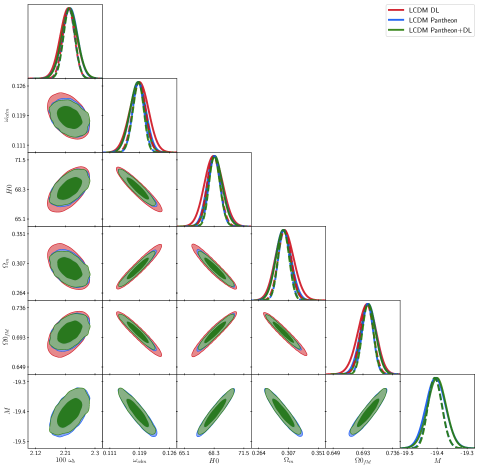
  Figure 5: Confidence contours for the $\Lambda$CDM model using Pantheon observational (blue), our RNN+BNN trained supernovae sample (DL) (red) and the join of these samples (Pantheon+DL) (green). One and two-dimensional posterior distribution are denoted by the solid line and the dashed line stands for the average likelihood distribution.

  Table 3: Best fits values for $\Lambda$CDM model using Pantheon sample.

  Parameters	Best-fit	mean$\pm\sigma$	95% lower	95% upper
  $100~{}w_{b}$	$2.224$	$2.226_{-0.025}^{+0.024}$	$2.177$	$2.274$
  $w_{cdm}$	$0.118$	$0.118_{-0.002}^{+0.002}$	$0.114$	$0.122$
  $M$	$-19.4$	$-19.4_{-0.023}^{+0.022}$	$-19.44$	$-19.35$
  $H_{0}$	$68.36$	$68.43_{-0.88}^{+0.81}$	$66.8$	$70.11$
  $\Omega_{m}$	$0.301$	$0.300_{-0.011}^{+0.011}$	$0.2776$	$0.322$
  $\Omega_{\Lambda}$	$0.700$	$0.670_{-0.011}^{+0.011}$	$0.678$	$0.722$

  
  
  

  Table 4: Best fits values for $\Lambda$CDM model using RNN+BNN supernovae (DL) sample.

  Parameter	Best-fit	mean$\pm\sigma$	95% lower	95% upper
  $100~{}w_{b}$	$2.223$	$2.223_{-0.025}^{+0.026}$	$2.172$	$2.274$
  $w_{cdm}$	$0.119$	$0.119_{-0.0024}^{+0.0024}$	$0.114$	$0.123$
  $H_{0}$	$68.28$	$68.29_{-1}^{+0.97}$	$66.33$	$70.27$
  $\Omega_{m}$	$0.302$	$0.302_{-0.014}^{+0.013}$	$0.275$	$0.329$
  $\Omega_{\Lambda}$	$0.698$	$0.698_{-0.013}^{+0.014}$	$0.671$	$0.724$

  
  
  

  Table 5: Best fits values for $\Lambda$CDM model using Pantheon+(RNN+BNN) supernovae (DL) sample.

  Parameter	Best-fit	mean$\pm\sigma$	95% lower	95% upper
  $100~{}w_{b}$	$2.224$	$2.226_{-0.025}^{+0.024}$	$2.177$	$2.275$
  $w_{cdm}$	$0.118$	$0.118_{-0.002}^{+0.002}$	$0.114$	$0.122$
  $M$	$-19.4$	$-19.4_{-0.022}^{+0.021}$	$-19.44$	$-19.35$
  $H_{0}$	$68.36$	$68.47_{-0.84}^{+0.77}$	$66.92$	$70.13$
  $\Omega_{m}$	$0.301$	$0.299_{-0.011}^{+0.011}$	$0.2771$	$0.320$
  $\Omega_{\Lambda}$	$0.699$	$0.700_{-0.011}^{+0.011}$	$0.680$	$0.723$

  
  
  

  

  

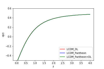
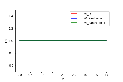
  Figure 6: Left: Cosmographic parameters for $\Lambda$CDM. Right: Deceleration parameter $q(z)$ using Pantheon observational (blue), our RNN+BNN trained supernovae sample (DL) (red) and the join of these samples (Pantheon+DL) (green). Left: Jerk parameter $j(z)$ using Pantheon observational (blue), our RNN+BNN trained supernovae sample (DL) (red) and the join of these samples (Pantheon+DL) (green).

• Case CPL. We present our statistical results using Eqs.(3.6)-(3.7)-(3.8) and the steps described in (i)-(ii)-(iii) above. For this model, we notice that our trained data overlaps the observational results in parameter spaces where there is no the dependence of the cosmological parameters. Suggesting that CPL is not a good option for $z>2.3$, the observational cutoff of Pantheon sample. When the samples are combined, the C.C is better with a correlation of the cosmological parameters at 1-$\sigma$ (see Figure 7). We compute the standard cosmographic parameter values at larger redshift (up to $z=4$) as it is shown in Figure 8 for the three samples. Notice that our RNN+BNN supernovae sample does not prefer the CPL model at low redshift, indicating that we should explore in detail another model. These latter results can be seen directly from the evolution of the $w(z)$ for each data sample under consideration (see Figure 17), where at low $z$, the model CPL using the RNN+BNN data trained violated the energy conditions. Also, this is indicated in the values of $H_{0}$, $\Omega_{m}$ and $\Omega_{\Lambda}$ that seems not converge (see Tables 6-7-8). At high redshifts, both parameters recover the standard scenario.

  

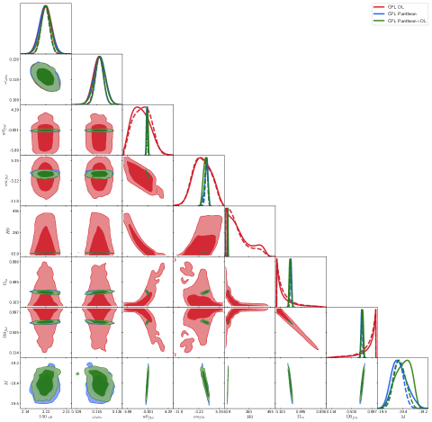
  Figure 7: Confidence contours for the CPL model using Pantheon observational (blue), our RNN+BNN trained supernovae sample (DL) (red) and the join of these samples (Pantheon+DL) (green). One and two-dimensional posterior distribution are denoted by the solid line and the dashed line stands for the average likelihood distribution.

  Table 6: Best fits values for CPL model using Pantheon sample.

  Parameter	Best-fit	mean$\pm\sigma$	95% lower	95% upper
  $100~{}w_{b}$	$2.219$	$2.223_{-0.026}^{+0.025}$	$2.172$	$2.275$
  $w_{cdm}$	$0.119$	$0.119_{-0.002}^{+0.002}$	$0.114$	$0.123$
  $w_{0}$	$-1.024$	$-0.985_{-0.17}^{+0.14}$	$-1.284$	$-0.641$
  $w_{a}$	$0.064$	$-0.158_{-0.54}^{+0.87}$	$-0.698$	$-0.711$
  $M$	$-19.4$	$-19.39_{-0.067}^{+0.052}$	$-19.52$	$-19.26$
  $H_{0}$	$68.41$	$68.64_{-2}^{+1.5}$	$65.03$	$72.47$
  $\Omega_{m}$	$0.301$	$0.230_{-0.015}^{+0.018}$	$0.265$	$0.334$
  $\Omega_{\Lambda}$	$0.699$	$0.700_{-0.018}^{+0.015}$	$0.666$	$0.735$

  
  
  

  Table 7: Best fits values for CPL model using RNN+BNN supernovae (DL) sample.

  Parameter	Best-fit	mean$\pm\sigma$	95% lower	95% upper
  $100~{}w_{b}$	$2.215$	$2.223_{-0.026}^{+0.026}$	$2.171$	$2.274$
  $w_{cdm}$	$0.117$	$0.1185_{-0.0024}^{+0.002}$	$0.1137$	$0.123$
  $w_{0}$	$0.077$	$-2.411_{-2.1}^{+2.7}$	$-4.511$	$0.289$
  $w_{a}$	$-0.055$	$-1.749_{-3.8}^{+4.1}$	$-8.729$	$5.576$
  $H_{0}$	$64.51$	$166.2_{-1.3e+02}^{+35}$	$37.82$	$379.8$
  $\Omega_{m}$	$0.335$	$0.154_{-0.15}^{+0.002}$	$0.004$	$0.156$
  $\Omega_{\Lambda}$	$0.665$	$0.846_{-0.002}^{+0.15}$	$0.844$	$0.996$

  
  
  

  Table 8: Best fits values for CPL model using Pantheon+(RNN+BNN) supernovae (DL) sample.

  Parameter	Best-fit	mean$\pm\sigma$	95% lower	95% upper
  $100~{}w_{b}$	$2.226$	$2.223_{-0.025}^{+0.025}$	$2.173$	$2.273$
  $w_{cdm}$	$0.118$	$0.118_{-0.002}^{+0.003}$	$0.113$	$0.123$
  $w_{0}$	$-1.006$	$-0.9189_{-0.17}^{+0.18}$	$-1.243$	$-0.6056$
  $w_{a}$	$-0.004$	$-0.508_{-0.79}^{+0.96}$	$-2.073$	$0.983$
  $M$	$-19.4$	$-19.36_{-0.059}^{+0.082}$	$-19.49$	$-19.24$
  $H_{0}$	$68.58$	$69.43_{-1.9}^{+2.2}$	$65.73$	$73.11$
  $\Omega_{m}$	$0.299$	$0.293_{-0.02}^{+0.018}$	$0.258$	$0.329$
  $\Omega_{\Lambda}$	$0.701$	$0.707_{-0.018}^{+0.02}$	$0.671$	$0.742$

  
  
  

  

  

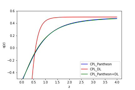
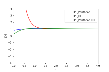
  Figure 8: Left: Cosmographic parameters for CPL. Right: Deceleration parameter $q(z)$ using Pantheon observational (blue), our RNN+BNN trained supernovae sample (DL) (red) and the join of these samples (Pantheon+DL) (green). Left: Jerk parameter $j(z)$ using Pantheon observational (blue), our RNN+BNN trained supernovae sample (DL) (red) and the join of these samples (Pantheon+DL) (green).

• Case RS. We present our statistical results using Eqs. (3.10)-(3.11)-(3.12) and the steps described in (i)-(ii)-(iii) above. For this model, we notice that our trained data continue overlapping with the observational results in parameter spaces where there is no dependence on the cosmological parameters. We notice that when samples are combined, the C.C is better with a correlation of the cosmological parameters at 1-$\sigma$ (see Figure 9). We compute the standard cosmographic parameter values at larger redshift (up to $z=4$) as it is shown in Figure 10 for the three samples. Here we notice that our RNN+BNN supernovae sample does have a preference for RS in comparison to the CPL model at low redshift, indicating that we should explore polynomials with $z^{2}$-factors. This is also indicated in the values of $H_{0}$, $\Omega_{m}$ and $\Omega_{\Lambda}$ that seems to converge better (see Tables 9-10-11). At high redshifts, both parameters recover the standard scenario. Interesting enough, in both CPL and RS cases, there is a deviation transition for $j$ in $z=[0.5,1]$, redshift regions where the Padé and Chebyshev could be considered.

  

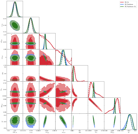
  Figure 9: Confidence contours for the RS model using Pantheon observational (blue), our RNN+BNN trained supernovae sample (DL) (red) and the join of these samples (Pantheon+DL) (green). One and two-dimensional posterior distribution are denoted by the solid line and the dashed line stands for the average likelihood distribution.

  Table 9: Best fits values for RS model using Pantheon sample.

  Parameter	Best-fit	mean$\pm\sigma$	95% lower	95% upper
  $100~{}w_{b}$	$2.224$	$2.222_{-0.026}^{+0.026}$	$2.171$	$2.273$
  $w_{cdm}$	$0.118$	$0.119_{-0.002}^{+0.002}$	$0.114$	$0.123$
  $w_{0}$	$-1.014$	$-0.986_{-0.12}^{+0.16}$	$-1.282$	$-0.717$
  $w_{a}$	$0.019$	$-0.100_{-0.4}^{+0.42}$	$-0.918$	$0.726$
  $M$	$-19.4$	$-19.39_{-0.062}^{+0.076}$	$-19.54$	$-19.25$
  $H_{0}$	$68.47$	$68.67_{-2}^{+2.2}$	$64.36$	$72.85$
  $\Omega_{m}$	$0.3$	$0.299_{-0.021}^{+0.018}$	$0.260$	$0.340$
  $\Omega_{\Lambda}$	$0.700$	$0.701_{-0.018}^{+0.021}$	$0.661$	$0.740$

  
  
  

  Table 10: Best fits values for RS model using RNN+BNN supernovae (DL) sample.

  Parameter	Best-fit	mean$\pm\sigma$	95% lower	95% upper
  $100~{}w_{b}$	$2.22$	$2.222_{-0.025}^{+0.025}$	$2.172$	$2.272$
  $w_{cdm}$	$0.119$	$0.119_{-0.003}^{+0.002}$	$0.114$	$0.123$
  $w_{0}$	$-1.738$	$-1.038_{-1.2}^{+0.36}$	$-2.22$	$0.4432$
  $w_{a}$	$1.721$	$-0.7272_{-1.5}^{+0.46}$	$-2.22$	$1.223$
  $H_{0}$	$177.4$	$81.61_{-35}^{+16}$	$41.4$	$126.4$
  $\Omega_{m}$	$0.045$	$0.274_{-0.2}^{+0.074}$	$0.045$	$0.611$
  $\Omega_{\Lambda}$	$0.955$	$0.725_{-0.074}^{+0.2}$	$0.389$	$0.955$

  
  
  

  Table 11: Best fits values for RS model using Pantheon+(RNN+BNN) supernovae (DL) sample.

  Parameter	Best-fit	mean$\pm\sigma$	95% lower	95% upper
  $100~{}\omega_{b}$	$2.223$	$2.223_{-0.026}^{+0.025}$	$2.172$	$2.275$
  $\omega_{cdm}$	$0.119$	$0.119_{-0.002}^{+0.003}$	$0.114$	$0.123$
  $w_{0}$	$-1.014$	$-0.950_{-0.13}^{+0.13}$	$-1.2$	$-0.709$
  $w_{a}$	$0.012$	$-0.203_{-0.31}^{+0.5}$	$-0.923$	$0.488$
  $M$	$-19.4$	$-19.37_{-0.040}^{+0.001}$	$-19.41$	$-19.36$
  $H_{0}$	$68.47$	$69.22_{-2.000}^{+1.900}$	$65.87$	$72.67$
  $\Omega_{m}$	$0.301$	$0.295_{-0.019}^{+0.017}$	$0.262$	$0.327$
  $\Omega_{0}$	$0.700$	$0.705_{-0.017}^{+0.019}$	$0.673$	$0.738$

  
  
  

  

  

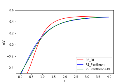
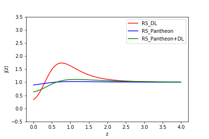
  Figure 10: Left: Cosmographic parameters for RS. Right: Deceleration parameter $q(z)$ using Pantheon observational (blue), our RNN+BNN trained supernovae sample (DL) (red) and the join of these samples (Pantheon+DL) (green). Left: Jerk parameter $j(z)$ using Pantheon observational (blue), our RNN+BNN trained supernovae sample (DL) (red) and the join of these samples (Pantheon+DL) (green).

  

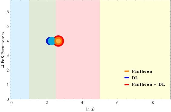
  Figure 11: Bayesian portrait for CPL and RS according to the number of free EoS parameters using the values given in Tables 6-7-8 and 9-10-11. The qualitative color regions represent Jeffrey’s scale as: strong evidence in favour of hypothesis model (light-yellow), moderate evidence in favour of hypothesis model (light-red), weak evidence for hypothesis model (light-green) and inconclusive evidence (light-blue). Each color in the plot legend indicates the sample used to calculated the value $\ln B_{ij}$ in comparison to $\Lambda$CDM model. For each sample, the light color circles denote the RS model and the darker color circles denote the CPL model. This option was selected since the models overlap statistically for the observational sample and the join sample.

5.2 $f(z)$CDM-like equations of state

To study $H_{0}$ tension issues using our EoS dark energy approximants-like, we consider as a fiducial prior Late Universe measurements as: $H_{0}=73.8\pm 1.1$km/s/Mpc from SH0ES $+$ H0LiCOW [1] in the following models:

• Case $f(z)$CDM Padé-like. For this model, consider (3.17), where, as we mentioned above, $P_{0}=1$ to recover Padé (2,2). To perform the numerical integration of this EoS, we consider a change of variable in terms of Padé approximants from $z=0$, where $P_{0}=-P_{1}/Q_{1}$, and then integrate up to $P_{0}=1$. In this manner we avoid any possible divergency due the Padé approximant. We notice a high correlation between the approximants of the model and the cosmological parameters for our three samples, see Figure 12 and Tables 12-13-14. The analyses with Pantheon and DL show positive bestfits values for the approximants $P_{1}$ and $P_{2}$, which is in agreement with the theoretical analysis from Figure 1. For the approximants $Q_{1}$ and $Q_{2}$ with contrary values in each sample cases, this is a remnant of the transition from a deceleration phase to an acceleration one as we can see from Figure 13. We observe also that the cosmographic parameters $q$ and $j$ are indistinguishable between each other for Pantheon+DL and Pantheon samples.

  

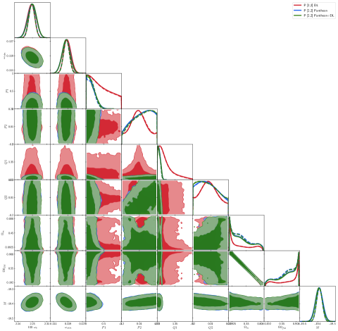
  Figure 12: Confidence contours for the $f(z)$CDM Padé-like model using Pantheon observational (blue), our RNN+BNN trained supernovae sample (DL) (red) and the join of these samples (Pantheon+DL) (green). One and two-dimensional posterior distribution are denoted by the solid line and the dashed line stands for the average likelihood distribution.

  Table 12: Best fits values for $f(z)$CDM Padé-like model using Pantheon sample.

  Parameters	Best-fit	mean$\pm\sigma$	95% lower	95% upper
  $100~{}w_{b}$	$2.222$	$2.225_{-0.025}^{+0.026}$	$2.174$	$2.275$
  $w_{cdm}$	$0.118$	$0.118_{-0.002}^{+0.002}$	$0.114$	$0.123$
  $P_{1}$	$0.183$	$0.156_{-0.16}^{+0.043}$	$1.462e-06$	$0.376$
  $P_{2}$	$0.040$	$0.035_{-0.061}^{+0.18}$	$-0.162$	$0.22$
  $Q_{1}$	$-0.204$	$-0.107_{-0.19}^{+0.053}$	$-0.3$	$0.131$
  $Q_{2}$	$0.0262$	$-0.013_{-0.19}^{+0.06}$	$-0.2$	$0.186$
  $M$	$-19.4$	$-19.4_{-0.029}^{+0.028}$	$-19.46$	$-19.34$
  $\Omega_{m}$	$0.251$	$0.311_{-0.31}^{+0.093}$	$0.001$	$0.404$
  $\Omega_{0}$	$0.749$	$0.688_{-0.093}^{+0.31}$	$0.595$	$0.998$

  
  
  

  Table 13: Best fits values for $f(z)$CDM Padé-like using RNN+BNN supernovae (DL) sample.

  Parameter	Best-fit	mean$\pm\sigma$	95% lower	95% upper
  $100~{}w_{b}$	$2.223$	$2.224_{-0.025}^{+0.025}$	$2.173$	$2.274$
  $w_{cdm}$	$0.118$	$0.118_{-0.002}^{+0.002}$	$0.114$	$0.123$
  $P_{1}$	$0.089$	$0.411_{-0.41}^{+0.14}$	$7.315e-06$	$0.921$
  $P_{2}$	$0.151$	$0.004_{-0.11}^{+0.099}$	$-0.188$	$0.196$
  $Q_{1}$	$-0.222$	$0.506_{-0.81}^{+0.14}$	$-0.3$	$2.07$
  $Q_{2}$	$-0.137$	$-0.004_{-0.14}^{+0.094}$	$-0.2$	$0.183$
  $\Omega_{m}$	$0.0142$	$0.28_{0.001}^{+0.002}$	$0.281$	$0.282$
  $\Omega_{0}$	$0.986$	$0.720_{0.001}^{+0.002}$	$0.721$	$0.722$

  
  
  

  Table 14: Best fits values for $f(z)$CDM Padé-like model using Pantheon+(RNN+BNN) supernovae (DL) sample.

  Parameter	Best-fit	mean$\pm\sigma$	95% lower	95% upper
  $100~{}w_{b}$	$2.221$	$2.226_{-0.026}^{+0.025}$	$2.176$	$2.276$
  $w_{cdm}$	$0.119$	$0.118_{-0.002}^{+0.002}$	$0.114$	$0.123$
  $P_{1}$	$0.108$	$0.154_{-0.15}^{+0.043}$	$1.897e-05$	$0.366$
  $P_{2}$	$-0.007$	$0.0370_{-0.06}^{+0.18}$	$-0.161$	$0.22$
  $Q_{1}$	$-0.163$	$-0.104_{-0.2}^{+0.055}$	$-0.3$	$0.135$
  $Q_{2}$	$0.055$	$-0.013_{-0.19}^{+0.061}$	$-0.203$	$0.048$
  $M$	$-19.4$	$-19.4_{-0.028}^{+0.027}$	$-19.45$	$-19.34$
  $\Omega_{m}$	$0.424$	$0.310_{-0.3}^{+0.092}$	$0.01$	$0.402$
  $\Omega_{0}$	$0.575$	$0.690_{-0.092}^{+0.3}$	$0.600$	$0.990$

  
  
  

  

  

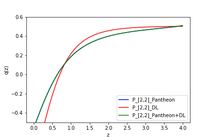
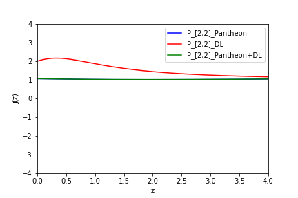
  Figure 13: Left: Cosmographic parameters for $f(z)$CDM Padé. Right: Deceleration parameter $q(z)$ using Pantheon observational (blue), our RNN+BNN trained supernovae sample (DL) (red) and the join of these samples (Pantheon+DL) (green). Left: Jerk parameter $j(z)$ using Pantheon observational (blue), our RNN+BNN trained supernovae sample (DL) (red) and the join of these samples (Pantheon+DL) (green).

• Case $f(z)$CDM Chebyshev-like. As in the latter case, for this model, consider (3.23), where $a_{3}=a_{1}/b_{1}$, to recover Chebyshev (2,1). To perform the numerical integration of the EoS, we consider a change of variable in terms of Chebyshev approximants from $a_{0}=0$, up to $a_{2}=-a_{1}/b_{1}$. In this manner we avoid any possible divergence and recover the original Chebyshev approximant. The results for this case are reported in Tables 15-16-17 and Figure 14. For this kind of polynomial $R_{(2,1)}$ we found a high correlation between approximants, but the confidence regions for the DL simulations gets to reproduce the same observational trend at $95\%$. The analyses with Pantheon and DL show a couple of positive bestfits values for the approximants $a_{1}$ and $a_{2}$ and negative values for $b_{1}$, in agreement with the theoretical analysis from Figure 1. From Figure 15 we notice deviations from $q$ and $j$ in comparison to the observational and join sample, but at high redshift, the three tested samples for this model are asymptotically approaching.

  

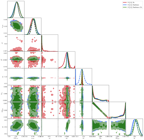
  Figure 14: Confidence contours for the $f(z)$CDM Chebyshev-like model using Pantheon observational (blue), our RNN+BNN trained supernovae sample (DL) (red) and the join of these samples (Pantheon+DL) (green). One and two-dimensional posterior distribution are denoted by the solid line and the dashed line stands for the average likelihood distribution.

  Table 15: Best fits values for $f(z)$CDM Chebyshev-like model using Pantheon sample.

  Parameter	Best-fit	mean$\pm\sigma$	95% lower	95% upper
  $100~{}w_{b}$	$2.222$	$2.223_{-0.026}^{+0.028}$	$2.168$	$2.277$
  $w_{cdm}$	$0.119$	$0.119_{-0.002}^{+0.002}$	$0.114$	$0.123$
  $a_{1}$	$0.026$	$0.013_{-0.065}^{+0.055}$	$-0.102$	$0.134$
  $a_{2}$	$-0.009$	$0.016_{-0.002}^{+0.001}$	$0.014$	$0.017$
  $b_{1}$	$0.587$	$0.140_{-0.73}^{+1.1}$	$-1.632$	$2.252$
  $M$	$-19.4$	$-19.39_{-0.005}^{+0.001}$	$-19.39$	$-19.39$
  $\Omega_{m}$	$0.134$	$0.248_{-0.005}^{+0.001}$	$0.243$	$0.245$
  $\Omega_{0}$	$0.866$	$0.752_{-0.005}^{+0.001}$	$0.745$	$0.753$

  
  
  

  Table 16: Best fits values for $f(z)$CDM Chebyshev-like using RNN+BNN supernovae (DL) sample.

  Parameter	Best-fit	mean$\pm\sigma$	95% lower	95% upper
  $100~{}w_{b}$	$2.22$	$2.225_{-0.024}^{+0.027}$	$2.175$	$2.278$
  $w_{cdm}$	$0.119$	$0.118_{-0.003}^{+0.002}$	$0.114$	$0.123$
  $a_{1}$	$-0.616$	$3.796_{-8.2}^{+2.8}$	$-4.404$	$6.596$
  $a_{2}$	$0.599$	$-0.059_{-0.13}^{+0.21}$	$-0.188$	$0.152$
  $b_{1}$	$-0.027$	$0.038_{-0.2}^{+0.14}$	$-0.162$	$0.178$
  $\Omega_{m}$	$0.256$	$0.291_{-0.002}^{+0.001}$	$0.289$	$0.292$
  $\Omega_{0}$	$0.744$	$0.708_{-0.002}^{+0.001}$	$0.706$	$0.709$

  
  
  

  Table 17: Best fits values for $f(z)$CDM Chebyshev-like model using Pantheon+(RNN+BNN) supernovae (DL) sample.

  Parameter	Best-fit	mean$\pm\sigma$	95% lower	95% upper
  $100~{}w_{b}$	$2.225$	$2.225_{-0.028}^{+0.024}$	$2.175$	$2.279$
  $w_{cdm}$	$0.119$	$0.118_{-0.002}^{+0.002}$	$0.114$	$0.123$
  $a_{1}$	$0.017$	$0.009_{-0.079}^{+0.07}$	$-0.149$	$0.162$
  $a_{2}$	$0.001$	$0.021_{-0.064}^{+0.046}$	$-0.119$	$0.251$
  $b_{1}$	$-1.618$	$-0.360_{-0.41}^{+0.71}$	$-0.77$	$0.350$
  $M$	$-19.4$	$-19.39_{-0.028}^{+0.026}$	$-19.44$	$-19.32$
  $\Omega_{m}$	$0.262$	$0.278_{-0.001}^{+0.001}$	$0.277$	$0.279$
  $\Omega_{0}$	$0.738$	$0.722_{-0.001}^{+0.001}$	$0.720$	$0.722$

  
  
  

  

  

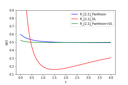
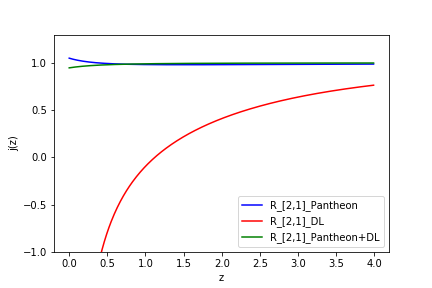
  Figure 15: Left: Cosmographic parameters for $f(z)$CDM Chebyshev. Right: Deceleration parameter $q(z)$ using Pantheon observational (blue), our RNN+BNN trained supernovae sample (DL) (red) and the join of these samples (Pantheon+DL) (green). Left: Jerk parameter $j(z)$ using Pantheon observational (blue), our RNN+BNN trained supernovae sample (DL) (red) and the join of these samples (Pantheon+DL) (green).

Model	$\chi^{2}$	$\bf{q_{0}}$	$\bf{j_{0}}$	$\ln{B_{ij}}$	AIC	BIC
$\Lambda$CDM	1028	$-0.551\pm 0.014$	$1.0$	-	-	-
CPL	1028	$-0.534\pm 0.308$	$0.790\pm 1.011$	2.637	1036	1055.4
RS	1028	$-0.536\pm 0.335$	$0.9\pm 1.312$	2.637	1036	1055.4
$f(z)$CDM Padé-like	1028	$-0.550\pm 0.354$	$1.063\pm 0.282$	2.637	1036	1055.94
$f(z)$CDM Chebyshev-like	1028	$0.599\pm 0.184$	$1.050\pm 0.460$	3.042	1038	1062.92

Table 18: Cosmological models and approximants using Pantheon sample. Column 1: cosmographic parameters values at 2-$\sigma$. Column 2: Bayes factor. Column 3 and 4: information criteria AIC and BIC, respectively.

Model	$\chi^{2}$	$\bf{q_{0}}$	$\bf{j_{0}}$	$\ln{B_{ij}}$	AIC	BIC
$\Lambda$CDM	7.991	$-0.550\pm 0.020$	$1.0$	-	-	-
CPL	2.75	$-1.721\pm 6.564$	$11.716\pm 66.16$	2.163	10.72	30.659
RS	3.81	$-0.632\pm 0.8272$	$0.344\pm 2.7626$	2.281	11.81	31.749
$f(z)$CDM Padé-like	7.97	$-0.910\pm 0.142$	$2.00\pm 0.601$	7.594	15.97	35.909
$f(z)$CDM Chebyshev-like	7.96	$4.358\pm 5.989$	$-7.643\pm 12.606$	7.588	17.96	42.884

Table 19: Cosmological models and approximants using trained DL Pantheon sample. Column 1: cosmographic parameters values at 2-$\sigma$. Column 2: Bayes factor. Column 3 and 4: information criteria AIC and BIC, respectively.

Model	$\chi^{2}$	$\bf{q_{0}}$	$\bf{j_{0}}$	$\ln{B_{ij}}$	AIC	BIC
$\Lambda$CDM	1035	$-0.551\pm 0.016$	$1.0$	-	-	-
CPL	1035	$-0.475\pm 0.380$	$0.224\pm 2.240$	2.637	1062.94	1043
RS	1035	$-0.505\pm 0.286$	$0.634\pm 1.309$	2.637	1062.94	1043
$f(z)$CDM Padé-like	1035	$-0.552\pm 0.35$	$1.070\pm 0.281$	2.637	1043	1062.94
$f(z)$CDM Chebyshev-like	1035	$0.525\pm 0.445$	$0.947\pm 0.605$	3.042	1045	1069.92

Table 20: Cosmological models and approximants using Pantheon + DL Pantheon samples. Column 1: cosmographic parameters values at 2-$\sigma$. Column 2: Bayes factor. Column 3 and 4: information criteria AIC and BIC, respectively.

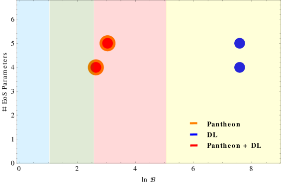
Figure 16: Bayesian portrait for Padé (2,2) and Chebyshev (2,1) according to the number of free EoS parameters using the values given in Tables 12-13-14 and 15-16-17. The qualitative color regions represent Jeffrey’s scale as: strong evidence in favour of hypothesis model (light-yellow), moderate evidence in favour of hypothesis model (light-red), weak evidence for hypothesis model (light-green) and inconclusive evidence (light-blue). Each color in the plot legend indicates the sample used to calculated the value $\ln B_{ij}$ in comparison to $\Lambda$CDM model. The Padé model lies in the y-axes line corresponding to four free parameters and the Chebyshev model lies in the y-axes line corresponding to five free parameters. Notice that the results obtained by using Pantheon and Pantheon+DL samples overlap statistically.

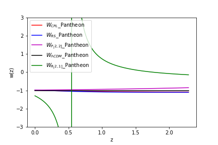
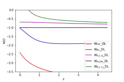
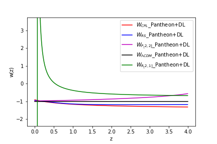
Figure 17: Equation of state for the standard cosmological models Sec.(3.1) and $f(z)$CDM cosmological models Secs.(3.2-3.3) obtained using the best fits reported for each sample and cases. $\Lambda$CDM model is denote by a solid black line, the standard models CPL and RS by solid red and blue lines, respectively and the Padé (2,2) and Chebyshev (2,1) models by purple and green lines, respectively.

6 Discussion

In this work, we presented a proposal that consists of an inverse cosmography approach from which we can compute a generic EoS without assuming directly a cosmographic series. In this approach it is possible to relax a couple of cosmography problems, as e.g truncation issues over the series/polynomials proposed. Also, we developed the study of the dark energy dynamics, without a $\Lambda$, by proposing suitable Padé or Chebyshev polynomials evolving with a cold dark matter (CDM) fluid. All these models were tested with current supernovae data and deep learning for supernovae trained samples. This machine learning architecture can train a homogeneous SNeIa sample in where the resulting dynamics of dark energy could lead to the necessity of another cosmological model different from $\Lambda$CDM. In this panorama, our inverse cosmography approach can fit very well since it is not necessary to consider higher-order corrections of the cosmography series to obtain a convergence best fit in comparison to the standard dark energy EoSs as our Bayesian analyses show (see Tables 18-19-20). The advantage to join current and trained supernovae sample is the density information data that we acquire in a redshift range of $0.01<z<4$, which is larger than the observable one. From the results of the Bayesian evidence, we notice that models polynomial-like, as Padé and Chebyshev lie in better significant regions in comparison to the standard ones (see Figure 11). Furthermore, $f(z)$CDM Padé-like and $f(z)$CDM Chebyshev-like are decisive in comparison to $\Lambda$CDM using DL sample (see Figure 16).

Now, from the perspective of the EoS’s (see Figure 17), we obtained the following results: in the case $f(z)$CDM Padé-like we obtain a dynamical EoS with a transition from $\Lambda$CDM to a quintessence scenario. A deviation of 1-$\sigma$ from the standard model can be observed using Pantheon and join sample. For this case, we notice that $f(z)$CDM Padé-like model does not have any divergence in the observational redshift range as it was reported in the mentioned references. Also, this model mimics $\Lambda$CDM at low redshift. On the contrary, $f(z)$CDM Chebyshev-like model does present a divergence at low redshift, but at high redshift starts to mimic $f(z)$CDM Padé-like model. Notice how all the tested models reproduce the theoretical scenarios reported in Figure 1.

Furthermore, up to the best of our knowledge, no CLASS + MontePython code adapted for cosmography has yet been developed. This process involves introducing directly the definition of the modulus distance and then deal with series divergencies. Meanwhile, using inverse cosmography it is possible to adapt easily the numerical codes and obtain a theoretical convergence. The inclusion of observable data from another nature that can give us information a higher redshifted universe will enrich the convergence of a series with more exotic polynomials. This future study will be reported elsewhere.

Appendix A Generic cosmographic parameters

In this Appendix we present the exact solutions of the cosmographic parameters for the models considered and in term of the standard cosmological parameters.

A.1 Chevallier-Polarski-Linder (CPL) case

With the inverse cosmography prescription (2.7)-(2.8)-(2.9), we can obtain the following cosmographic parameters for this model as follow:

$$q(z) = \frac{\left(\Omega_{m}-1\right)(z+1)^{3\left(w_{a}+w_{0}\right)}\left(3zw_{a}+3w_{0}(z+1)+z+1\right)-(z+1)\Omega_{m}e^{\frac{3zw_{a}}{z+1}}}{2\left(\Omega_{m}-1\right)(z+1)^{3w_{a}+3w_{0}+1}-2(z+1)\Omega_{m}e^{\frac{3zw_{a}}{z+1}}},$$ (A.1)

$$j(z) = \frac{\left(\Omega_{m}-1\right)\left(9z^{2}w_{a}^{2}+3(3z+1)(z+1)w_{a}+2(z+1)^{2}\right)(z+1)^{3\left(w_{a}+w_{0}\right)}}{2(z+1)^{2}\left(\left(\Omega_{m}-1\right)(z+1)^{3\left(w_{a}+w_{0}\right)}-\Omega_{m}e^{\frac{3zw_{a}}{z+1}}\right)}$$ (A.2)

$$+\frac{9w_{0}\left(\Omega_{m}-1\right)\left(2zw_{a}+z+1\right)(z+1)^{3w_{a}+3w_{0}+1}}{2(z+1)^{2}\left(\left(\Omega_{m}-1\right)(z+1)^{3\left(w_{a}+w_{0}\right)}-\Omega_{m}e^{\frac{3zw_{a}}{z+1}}\right)}$$

$$+\frac{9w_{0}^{2}\left(\Omega_{m}-1\right)(z+1)^{3w_{a}+3w_{0}+2}-2(z+1)^{2}\Omega_{m}e^{\frac{3zw_{a}}{z+1}}}{2(z+1)^{2}\left(\left(\Omega_{m}-1\right)(z+1)^{3\left(w_{a}+w_{0}\right)}-\Omega_{m}e^{\frac{3zw_{a}}{z+1}}\right)},$$

$$s(z) = \left[\frac{\left(\Omega_{m}-1\right)(z+1)^{3\left(w_{a}+w_{0}\right)}}{2\left(\Omega_{m}-1\right)(z+1)^{3w_{a}+3w_{0}+4}-2(z+1)^{4}\Omega_{m}e^{\frac{3zw_{a}}{z+1}}}\right]$$ (A.3)

$$\times(-9z^{3}w_{a}^{3}+(z+1)^{2}w_{a}\left(-9w_{0}\left(3w_{0}z-2(z-1)z+1\right)+9z^{2}+z-2\right)$$

$$+9z(z+1)w_{a}^{2}\left(-3w_{0}z+(z-1)z-1\right)$$

$$+\left(9w_{0}\left(w_{0}+1\right)+2\right)(z+1)^{3}\left(z-w_{0}\right))-2z(z+1)^{3}\Omega_{m}e^{\frac{3zw_{a}}{z+1}},$$

A.2 Redshift squared (RS) case

With the inverse cosmography prescription (2.7)-(2.8)-(2.9), we can obtain the following cosmographic parameters for this model as follow:

$$\frac{2}{3}(q(z)+1) = \frac{\left(\Omega_{m}-\left(\Omega_{m}-1\right)(z+1)^{3w_{0}}\left(z^{2}+1\right)^{\frac{3w_{a}}{2}-1}\left(z(z+1)w_{a}+\left(w_{0}+1\right)\left(z^{2}+1\right)\right)\right)}{\Omega_{m}-\left(\Omega_{m}-1\right)(z+1)^{3w_{0}}\left(z^{2}+1\right)^{\frac{3w_{a}}{2}}},\quad\quad$$ (A.4)

$$2j(z) = \frac{3\left(\Omega_{m}-1\right)(z+1)^{3w_{0}}}{\left(z^{2}+1\right)^{2}\left(\left(\Omega_{m}-1\right)(z+1)^{3w_{0}}-\Omega_{m}\left(z^{2}+1\right)^{-\frac{3w_{a}}{2}}\right)}$$ (A.5)

$$\times((z+1)w_{a}\left(6w_{0}\left(z^{3}+z\right)+z(z(3z-1)+5)+1\right)$$

$$+3z^{2}(z+1)^{2}w_{a}^{2}+3w_{0}\left(w_{0}+1\right)\left(z^{2}+1\right)^{2})+2,$$

$$s(z) = \frac{3\left(\Omega_{m}-1\right)(z+1)^{3w_{0}}}{6(z+1)\left(z^{2}+1\right)^{3}\left(\left(\Omega_{m}-1\right)(z+1)^{3w_{0}}\left(z^{2}+1\right)^{\frac{3w_{a}}{2}}-\Omega_{m}\right)}$$ (A.6)

$$\times\left(z^{2}+1\right)^{\frac{3w_{a}}{2}}(-9z^{3}(z+1)^{3}w_{a}^{3}+9z(z+1)^{2}w_{a}^{2}(-3w_{0}\left(z^{3}+z\right)$$

$$+z(z((z-1)z+2)-3)-1)+(z+1)w_{a}(9w_{0}\left(z^{2}+1\right)$$

$$\times\left(-3w_{0}\left(z^{3}+z\right)+z(z(2(z-1)z+3)-4)-1\right)$$

$$+z(z(z(z(z(9z-5)+26)-8)+27)-3)-6)$$

$$+\left(9w_{0}\left(w_{0}+1\right)+2\right)\left(z^{2}+1\right)^{3}\left(z-w_{0}\right))-6z\left(z^{2}+1\right)^{3}\Omega_{m}.$$

A.3 $f(z)$CDM Padé-like case

With the inverse cosmography prescription (2.7)-(2.8)-(2.9), we can obtain the following cosmographic parameters for this model as follow:

$$q(z) = \frac{(z+1)\left(3(z+1)^{2}\Omega_{m}+\frac{\Omega_{p}\left(P_{1}\left(Q_{2}z^{2}-1\right)+P_{2}z\left(Q_{1}z+2\right)-2Q_{2}z-Q_{1}\right)}{\left(z\left(Q_{2}z+Q_{1}\right)+1\right){}^{2}}\right)}{2\left((z+1)^{3}\Omega_{m}+\frac{\Omega_{p}\left(P_{2}z^{2}-P_{1}z+1\right)}{z\left(Q_{2}z+Q_{1}\right)+1}\right)}-1,$$ (A.7)

$$\frac{j(z)}{(z+1)\Omega_{p}}-1 = \frac{P_{1}\left(Q_{2}^{2}(-(2z+1))z^{3}+Q_{1}\left(-Q_{2}z^{3}+2z+1\right)+3Q_{2}(z+1)z+1\right)}{\left(z\left(Q_{2}z+Q_{1}\right)+1\right){}^{2}\left((z+1)^{3}\Omega_{m}\left(z\left(Q_{2}z+Q_{1}\right)+1\right)+\Omega_{p}\left(P_{2}z^{2}-P_{1}z+1\right)\right)}$$ (A.8)

$$+\frac{P_{2}\left(z^{2}\left(-Q_{1}\left(Q_{1}z+3\right)-Q_{2}\left(Q_{1}(2z+1)z+5z+3\right)\right)-z+1\right)}{\left(z\left(Q_{2}z+Q_{1}\right)+1\right){}^{2}\left((z+1)^{3}\Omega_{m}\left(z\left(Q_{2}z+Q_{1}\right)+1\right)+\Omega_{p}\left(P_{2}z^{2}-P_{1}z+1\right)\right)}$$

$$+\frac{Q_{2}^{2}z^{2}(5z+3)+Q_{2}\left(3Q_{1}(2z+1)z+z-1\right)+Q_{1}\left(2Q_{1}z+Q_{1}+1\right))}{\left(z\left(Q_{2}z+Q_{1}\right)+1\right){}^{2}\left((z+1)^{3}\Omega_{m}\left(z\left(Q_{2}z+Q_{1}\right)+1\right)+\Omega_{p}\left(P_{2}z^{2}-P_{1}z+1\right)\right)},\quad\quad\quad$$

$$\frac{1-s(z)}{(z+1)} = \frac{(z+1)\Omega_{m}\left(z\left(Q_{2}z+Q_{1}\right)+1\right){}^{4}}{\left(z\left(Q_{2}z+Q_{1}\right)+1\right){}^{3}\left((z+1)^{3}\Omega_{m}\left(z\left(Q_{2}z+Q_{1}\right)+1\right)+\Omega_{p}\left(P_{2}z^{2}-P_{1}z+1\right)\right)}$$ (A.9)

$$+\frac{\Omega_{p}(Q_{2}^{3}z^{3}\left(P_{1}z(2z(z+1)+1)-z(5z+7)-4\right)}{\left(z\left(Q_{2}z+Q_{1}\right)+1\right){}^{3}\left((z+1)^{3}\Omega_{m}\left(z\left(Q_{2}z+Q_{1}\right)+1\right)+\Omega_{p}\left(P_{2}z^{2}-P_{1}z+1\right)\right)}$$

$$+\frac{Q_{2}^{2}z\left(P_{1}z\left(Q_{1}(3z+1)z^{2}-(z+8)z-6\right)-Q_{1}(z(11z+12)+6)z-6z^{2}+2z+4\right)}{\left(z\left(Q_{2}z+Q_{1}\right)+1\right){}^{3}\left((z+1)^{3}\Omega_{m}\left(z\left(Q_{2}z+Q_{1}\right)+1\right)+\Omega_{p}\left(P_{2}z^{2}-P_{1}z+1\right)\right)}$$

$$+\frac{Q_{2}(P_{1}\left(Q_{1}^{2}z^{4}-4Q_{1}(z+1)^{2}z-2(2z+1)z+1\right)}{\left(z\left(Q_{2}z+Q_{1}\right)+1\right){}^{3}\left((z+1)^{3}\Omega_{m}\left(z\left(Q_{2}z+Q_{1}\right)+1\right)+\Omega_{p}\left(P_{2}z^{2}-P_{1}z+1\right)\right)}$$

$$+\frac{2Q_{1}\left(-2Q_{1}(2z(z+1)+1)z-4z^{2}+1\right)-z)+P_{2}(Q_{2}^{2}z^{3}(Q_{1}z(2z(z+1)+1)}{\left(z\left(Q_{2}z+Q_{1}\right)+1\right){}^{3}\left((z+1)^{3}\Omega_{m}\left(z\left(Q_{2}z+Q_{1}\right)+1\right)+\Omega_{p}\left(P_{2}z^{2}-P_{1}z+1\right)\right)}$$

$$+\frac{z(5z+7)+4)+Q_{2}z\left(Q_{1}z^{2}\left(Q_{1}(3z+1)z+10z+4\right)+2(z-1)(3z+2)\right)}{\left(z\left(Q_{2}z+Q_{1}\right)+1\right){}^{3}\left((z+1)^{3}\Omega_{m}\left(z\left(Q_{2}z+Q_{1}\right)+1\right)+\Omega_{p}\left(P_{2}z^{2}-P_{1}z+1\right)\right)}$$

$$+\frac{Q_{1}\left(Q_{1}z^{3}\left(Q_{1}z+4\right)+4z^{2}-2z-1\right)+z)}{\left(z\left(Q_{2}z+Q_{1}\right)+1\right){}^{3}\left((z+1)^{3}\Omega_{m}\left(z\left(Q_{2}z+Q_{1}\right)+1\right)+\Omega_{p}\left(P_{2}z^{2}-P_{1}z+1\right)\right)}$$

$$+\frac{Q_{1}\left(-\left(P_{1}+Q_{1}\right)\left(Q_{1}(2z(z+1)+1)+3z\right)-Q_{1}\right)}{\left(z\left(Q_{2}z+Q_{1}\right)+1\right){}^{3}\left((z+1)^{3}\Omega_{m}\left(z\left(Q_{2}z+Q_{1}\right)+1\right)+\Omega_{p}\left(P_{2}z^{2}-P_{1}z+1\right)\right)}$$

$$-\frac{\left(P_{1}+1\right)Q_{1}+Q_{2})-\left(P_{1}+P_{2}\right)\Omega_{p}}{\left(z\left(Q_{2}z+Q_{1}\right)+1\right){}^{3}\left((z+1)^{3}\Omega_{m}\left(z\left(Q_{2}z+Q_{1}\right)+1\right)+\Omega_{p}\left(P_{2}z^{2}-P_{1}z+1\right)\right)},\quad\quad\quad\quad$$

A.4 $f(z)$CDM Chebyshev-like case

With the inverse cosmography prescription (2.7)-(2.8)-(2.9), we can obtain the following cosmographic parameters for this model as follow:

$$q(z) = \frac{(z+1)\left(\Omega_{p}\left(2a_{2}z\left(b_{1}z+2\right)-a_{3}b_{1}+a_{1}\right)+3(z+1)^{2}\left(b_{1}z+1\right){}^{2}\Omega_{m}\right)}{2\left(b_{1}z+1\right)\left(\left(z\left(2a_{2}z+a_{1}\right)+a_{3}\right)\Omega_{p}+(z+1)^{3}\left(b_{1}z+1\right)\Omega_{m}\right)}-1,$$ (A.10)

$$j(z) = \frac{\Omega_{p}(a_{1}\left(b_{1}\left(b_{1}z^{3}-3z-1\right)-1\right)+b_{1}(a_{3}\left(b_{1}(3z(z+1)+1)+3z+1\right)}{\left(b_{1}z+1\right){}^{2}\left(\left(z\left(2a_{2}z+a_{1}\right)+a_{3}\right)\Omega_{p}+(z+1)^{3}\left(b_{1}z+1\right)\Omega_{m}\right)}$$ (A.11)

$$-\frac{2a_{2}z^{2}\left(b_{1}z+z+3\right))+2a_{2}+a_{3})+(z+1)^{3}\left(b_{1}z+1\right){}^{3}\Omega_{m}}{\left(b_{1}z+1\right){}^{2}\left(\left(z\left(2a_{2}z+a_{1}\right)+a_{3}\right)\Omega_{p}+(z+1)^{3}\left(b_{1}z+1\right)\Omega_{m}\right)},$$

$$s(z) = \frac{\Omega_{p}(a_{1}\left(b_{1}\left(b_{1}z^{3}-3z-1\right)-1\right)+b_{1}(a_{3}\left(b_{1}(3z(z+1)+1)+3z+1\right)}{\left(b_{1}z+1\right){}^{2}\left(\left(z\left(2a_{2}z+a_{1}\right)+a_{3}\right)\Omega_{p}+(z+1)^{3}\left(b_{1}z+1\right)\Omega_{m}\right)}$$ (A.12)

$$-\frac{2a_{2}z^{2}\left(b_{1}z+z+3\right))+2a_{2}+a_{3})+(z+1)^{3}\left(b_{1}z+1\right){}^{3}\Omega_{m}}{\left(b_{1}z+1\right){}^{2}\left(\left(z\left(2a_{2}z+a_{1}\right)+a_{3}\right)\Omega_{p}+(z+1)^{3}\left(b_{1}z+1\right)\Omega_{m}\right)}.$$

References

- [1] L. Verde, T. Treu and A. G. Riess, Nature Astronomy 2019 doi:10.1038/s41550-019-0902-0 [arXiv:1907.10625 [astro-ph.CO]].
- [2] Y. L. Bolotin, V. A. Cherkaskiy, O. Y. Ivashtenko, M. I. Konchatnyi and L. G. Zazunov, arXiv:1812.02394 [gr-qc].
- [3] S. Capozziello, M. De Laurentis, O. Luongo and A. Ruggeri, Galaxies 1, 216 (2013) doi:10.3390/galaxies1030216 [arXiv:1312.1825 [gr-qc]].
- [4] C. Escamilla-Rivera and S. Capozziello, Int. J. Mod. Phys. D 28, no. 12, 1950154 (2019) doi:10.1142/S0218271819501542 [arXiv:1905.04602 [gr-qc]].
- [5] C. Escamilla-Rivera, M. A. C. Quintero and S. Capozziello, JCAP 03 (2020) no.03, 008 doi:10.1088/1475-7516/2020/03/008 [arXiv:1910.02788 [astro-ph.CO]].
- [6] S. Capozziello, R. D’Agostino and O. Luongo, Int. J. Mod. Phys. D 28, no. 10, 1930016 (2019) doi:10.1142/S0218271819300167 [arXiv:1904.01427 [gr-qc]].
- [7] https://www.desi.lbl.gov https://www.lsst.org
- [8] D. J. Schlegel et al., arXiv:1907.11171 [astro-ph.IM].
- [9] Bowman, J., Rogers, A., Monsalve, R. et al. Nature 555, 67–70 (2018).
- [10] M. Corman, C. Escamilla-Rivera and M. Hendry, [arXiv:2004.04009 [astro-ph.CO]].
- [11] [LIGO Scientific and Virgo], [arXiv:2004.08342 [astro-ph.HE]].
- [12] C. Escamilla-Rivera and J. C. Fabris, Galaxies 4, no. 4, 76 (2016) doi:10.3390/galaxies4040076 [arXiv:1511.07066 [astro-ph.CO]].
- [13] E. K. Li, M. Du and L. Xu, Mon. Not. Roy. Astron. Soc. 491, no. 4, 4960 (2020) doi:10.1093/mnras/stz3308
- [14] C. Gruber and O. Luongo, Phys. Rev. D 89, no. 10, 103506 (2014) doi:10.1103/PhysRevD.89.103506
- [15] S. Capozziello, R. D’Agostino and O. Luongo, Mon. Not. Roy. Astron. Soc. 476, no. 3, 3924 (2018) doi:10.1093/mnras/sty422 [arXiv:1712.04380 [astro-ph.CO]].
- [16] A. Aviles, C. Gruber, O. Luongo and H. Quevedo, Phys. Rev. D 86, 123516 (2012) doi:10.1103/PhysRevD.86.123516 [arXiv:1204.2007 [astro-ph.CO]].
- [17] M. Benetti and S. Capozziello, JCAP 1912, no. 12, 008 (2019) doi:10.1088/1475-7516/2019/12/008 [arXiv:1910.09975 [astro-ph.CO]].
- [18] C. Escamilla-Rivera, Galaxies 4 (2016) 8.
- [19] M. Chevallier, D. Polarski, Int. J. Mod. Phys. D 10 (2001) 213.
- [20] E.V. Linder, Gen. Rel. Grav. 40 (2008) 329.
- [21] E.M. Jr. Barboza, J.S. Alcaniz, Phys. Lett. B 666 (2008) 415.
- [22] A. Aviles, J. Klapp and O. Luongo, Phys. Dark Univ. 17, 25 (2017) doi:10.1016/j.dark.2017.07.002 [arXiv:1606.09195 [astro-ph.CO]].
- [23] S. Capozziello, Ruchika and A. A. Sen, Mon. Not. Roy. Astron. Soc. 484, 4484 (2019) doi:10.1093/mnras/stz176 [arXiv:1806.03943 [astro-ph.CO]].
- [24] V. Vitagliano, J. Q. Xia, S. Liberati and M. Viel, JCAP 03, 005 (2010) doi:10.1088/1475-7516/2010/03/005 [arXiv:0911.1249 [astro-ph.CO]].
- [25] A. R. Liddle, Mon. Not. Roy. Astron. Soc. 351, L49 (2004) doi:10.1111/j.1365-2966.2004.08033.x [astro-ph/0401198].
- [26] H. Jeffreys, Theory of Probability, 3rd ed.; Oxford University Press: Oxford, United Kingdom. 1998.
- [27] D. M. Scolnic et al., Astrophys. J. 859 (2018) 101