DTR Bandit: Learning to Make Response-Adaptive Decisions With Low Regret

Abstract

Dynamic treatment regimes (DTRs) are personalized, adaptive, multi-stage treatment plans that adapt treatment decisions both to an individual’s initial features and to intermediate outcomes and features at each subsequent stage, which are affected by decisions in prior stages. Examples include personalized first- and second-line treatments of chronic conditions like diabetes, cancer, and depression, which adapt to patient response to first-line treatment, disease progression, and individual characteristics. While existing literature mostly focuses on estimating the optimal DTR from offline data such as from sequentially randomized trials, we study the problem of developing the optimal DTR in an online manner, where the interaction with each individual affect both our cumulative reward and our data collection for future learning. We term this the DTR bandit problem. We propose a novel algorithm that, by carefully balancing exploration and exploitation, is guaranteed to achieve rate-optimal regret when the transition and reward models are linear. We demonstrate our algorithm and its benefits both in synthetic experiments and in a case study of adaptive treatment of major depressive disorder using real-world data.

Keywords: dynamic treatment regimes; online learning; adaptive intervention; $Q$-learning; personalized decision making.

1 Introduction

Contextual bandits, where personalized decisions are made sequentially and simultaneously with data collection, are increasingly used to address important decision making problems where data is limited and expensive to collect, with applications in product recommendation (Li et al. 2011), revenue management (Qiang and Bayati 2016), policymaking (Athey et al. 2018), and personalized medicine (Tewari and Murphy 2017). Bandit algorithms are also increasingly being considered in place of classic randomized trials in order to improve both learning and the outcomes for study participants (Villar et al. 2015, Athey et al. 2018).

But, in many cases decisions are not a one-and-done proposition and there is often a crucial opportunity to adapt to a unit’s response to initial treatment. Generally, a more conservative or more commonly effective treatment is often used at first, reverting to more intensive or more unique treatment if the patient’s condition does not respond to the initial intervention or dialing treatment back if the condition is in remission. Figure 1, for example, shows a personalized and adaptive treatment plan for the treatment of pediatric attention deficit hyperactivity disorder (ADHD) proposed by Pelham and Fabiano (2008). These adaptive treatment plans are called dynamic treatment regimes (DTRs; Murphy 2003). Crucially, in DTRs, the initial treatment choice not only affects the initial outcome, but also a subject’s features in future stages, which may further affect future decisions and outcomes. Therefore, successful learning of DTRs hinges on accurately learning both the outcome and the transition dynamics and their dependence on subject’s features.

Figure 1: A simple DTR for the treatment of attention deficit hyperactivity disorder (ADHD). B-mod stands for behavioral modification therapy.

Traditionally, DTRs are estimated offline, usually from data collected by sequential multiple assignment randomized trials (SMARTs), which randomize assignment at each decision point. Many offline learning methods for DTRs have been proposed, which assume that we have access to the collection of observed trajectories for all patients who participated in the study. However, sequential randomized trials are usually costly and limited in size in practice, especially in healthcare domains. Thus, it would be attractive to use algorithms that learn an effective DTR in an online manner while ensuring subjects have good outcomes, much like the contextual bandit algorithms but being able to be response-adaptive at the unit level. Adaptivity is incredibly crucial in practice: while contextual bandits can personalize treatments to individuals’ baseline characteristics such as age, weight, comorbidities, etc., these features’ predictive ability pales in comparison to the informativeness of an individual’s actual response to an actual treatment.

In this paper, we study efficient online learning algorithms for optimal DTRs when the $Q$ functions are linear. As in contextual bandits, from each unit we interact with, we only observe bandit feedback, i.e., only the rewards of the actions taken and never that of the others, so we face the trade-off between exploration and exploitation: we are motivated to apply the current-best DTR so to collect the highest reward for the current unit, but we also need to explore other treatments for fear of missing better options for future units due to lack of data. Unlike contextual bandits, our decisions not only impact the immediate reward and which arm we observe at the present context for use in future learning, but they also impact both the possible reward in future stages for the same unit and the possible context at which we may obtain new data on future-stage reward structure. Our proposed algorithm tackles the trade-off between exploration and exploitation by carefully balancing the two imperatives and maintaining two sets of parameter estimators (one unbiased but imprecise, one biased but much more precise) to use in different context regions (inspired by Goldenshluger and Zeevi 2013). We prove that, under a sharp margin condition (i.e., $\alpha=1$ in Assumption 2 below), our algorithm only incurs $O(\log T)$ regret after interacting with $T$ units, compared to the oracle policy that knows the true reward and transition models exactly. Our result is rate optimal and comparable to regret rates in the one-stage linear-response bandit problem where we may treat each unit only once.

1.1 Related Literature

Dynamic Treatment Regimes.

DTRs generalize individualized treatment regimes (ITRs; Kallus 2018, Athey and Wager 2021, Qian and Murphy 2011, Zhao et al. 2012), which personalize single treatment interventions based on baseline unit features. In DTR models, additional interventions are made and can be tailored to the patient’s time-varying features, which may be impacted by previous interventions. A number of methods have been proposed to estimate the optimal DTR from batched data from either randomized trials or observational studies, including potential outcome imputation (Murphy et al. 2001), likelihood-based methods (Thall et al. 2007), $A$-learning (Murphy 2003, Schulte et al. 2014), and weight-based methods (Zhao et al. 2015, Zhang et al. 2013, Jiang et al. 2019), among others. Our work leverages ideas from $Q$-learning, which has been used for learning DTRs offline from both randomized trial data (Zhao et al. 2009, Chakraborty et al. 2010, Shortreed et al. 2011, Song et al. 2015) and observational data (Moodie et al. 2014). For a more complete review of DTR methods, see Chakraborty and Moodie (2013).

Efficient Reinforcement Learning (RL).

Online algorithms and regret analysis appear rarely in the DTR literature. A closely related topic is studied in regret-efficient exploration in episodic RL problems. The tabular RL case, where both state and action spaces are finite, is well-studied in the literature (e.g., Azar et al. 2017). However, the state space (which corresponds to units’ features in DTR problems) is usually enormous or even infinite in real-world applications, which makes the tabular algorithms (whose regret grows polynomially in the number of states) untenable in practice. Thus, effectively modeling the problem structure is necessary. Jin et al. (2019) proposed an efficient RL algorithm with linear function approximation (LSVI-UCB) and proved $O(\sqrt{T})$ regret. The current work differs from Jin et al. (2019) by introducing the margin condition to the DTR problem, which allows for much lower regret rate when feature distributions are not arbitrarily concentrated near the decision boundary, as would indeed not occur in practice. In the context of RL with function approximation, our paper is the first to leverage such a condition to obtain logarithmic regret rates, which are faster than square-root rates that are minimax optimal in the absence of a margin condition. Moreover, we consider the new problem of delayed feedback in Appendix C. Beyond regret minimization, some recent work studied other aspects of RL with linear/low-rank MDPs, including policy learning (Yang and Wang 2019) and representation learning (Agarwal et al. 2020).

Contextual Bandits.

Contextual bandits extends multi-armed bandits (Lai and Robbins 1985) by introducing observations of side information at each time point (e.g., Auer 2002). While some literature makes no assumption about the context generating process and allows for adversarially chosen contexts (e.g., Beygelzimer et al. 2011), this can be overly pessimistic in real-world scenarios and inevitably leads to high regret. Thus, another line of literature considers the stochastic contextual bandit problem, which assumes that contexts and rewards are drawn i.i.d. from a stationary but unknown distribution (e.g., Dudik et al. 2011). We will focus on the stochastic setting in this paper.

The margin condition, which has been introduced to characterize the hardness of classification problems (Mammen and Tsybakov 1999), has been used in stochastic contextual bandits in Rigollet and Zeevi (2010), Goldenshluger and Zeevi (2013), Hu et al. (2022), Bastani and Bayati (2020), among others. The margin condition parameter (usually denoted as $\alpha\geq 0$) quantifies the concentration of contexts near the decision boundary between arms and crucially determines the learning difficulty of bandit problems. Among these, Rigollet and Zeevi (2010), Perchet and Rigollet (2013), Hu et al. (2022) assume non-parametric relationships between rewards and covariates. Nonparametric algorithms may perform poorly in moderate to high dimensions due to the curse of dimension, so much of the literature focuses on the case where the rewards are parametric – particularly, linear – functions of the observed contexts. Under the linear model, Goldenshluger and Zeevi (2013) achieve optimal $O(\log T)$ regret under a sharp margin ($\alpha=1$). Bastani et al. (2021) show that the analysis techniques can be easily extended to general margin conditions.

1.2 Organization

The rest of the paper is organized as follows. In Section 2, we formally introduce the DTR bandit problem and assumptions. We describes our proposed algorithm in Section 3. In Section 4, we analyze our algorithm theoretically: we derive an upper bound on the regret of our algorithm, and we show a matching lower bound on the regret of any algorithm. In Section 5 we evaluate the empirical performance of our algorithm on both synthetic data and a real-world sequenced randomized trial on treatment regimes for patients with major depressive disorder. We conclude our paper and discuss future directions in Section 6.

1.3 Notation

We use $\|\cdot\|$ to represent the Euclidean norm of vectors and the spectral norm of matrices, $\|\cdot\|_{1}$ to represent the $L_{1}$ norm of vectors, and $\|\cdot\|_{\infty}$ to represent the infinity norm of vectors. For any integer $n$, let $[n]$ denote the set $\{1,\dots,n\}$. For two scalers $a,b\in\mathbb{R}$, let $a\wedge b=\min\{a,b\}$ and $a\vee b=\max\{a,b\}$. For an event $A$, the indicator variable $\mathbb{I}(A)$ is equal to $1$ if $A$ is true and $0$ otherwise. For a set $S$, its cardinality is denoted as $|S|$. For a matrix $\mathcal{A}$, its minimum and maximum eigenvalues are denoted as $\lambda_{\min}(\mathcal{A})$, $\lambda_{\max}(\mathcal{A})$, respectively. For two functions $f_{1}(T)>0$ and $f_{2}(T)>0$, we use the standard notation for asymptotic order: $f_{1}(T)=O(f_{2}(T))$ represents $\limsup_{T\to\infty}f_{1}(T)/f_{2}(T)<\infty$, $f_{1}(T)=\Omega(f_{2}(T))$ represents $\liminf_{T\to\infty}f_{1}(T)/f_{2}(T)>0$, and $f_{1}(T)=\Theta(f_{2}(T))$ represents simultaneously $f_{1}(T)=\Omega(f_{2}(T))$ and $f_{1}(T)=O(f_{2}(T))$.

2 The DTR Bandit Problem

We now formally formulate the DTR bandit problem. For simplicity, we focus on the two-armed two-stage DTR bandits. We present the extension to the general multi-armed problem in Appendix D and discuss the $M$-stage problem in Section 6.

2.1 Problem Setup

The DTR bandit problem proceeds in rounds indexed by $t$. For $t=1,2,\dots$, nature draws a potential trajectory $\left\{\mathbf{X}_{t,1},\mathbf{X}_{t,2}\left(a_{1}\right),\mathbf{X}_{t,3}\left(a_{1},a_{2}\right)\right\}_{a_{1}\in[2],a_{2}\in[2]}$ i.i.d. from a fixed but unknown distribution $\mathcal{P}$. In the first stage of each round, the decision maker observes the initial context $\mathbf{X}_{t,1}\in\mathcal{X}_{1}\subseteq\mathbb{R}^{p_{1}}$ and pulls an arm $A_{t,1}\in[2]$ according to the observed context and the data collected so far. They then obtain an updated context $\mathbf{X}_{t,2}=\mathbf{X}_{t,2}(A_{t,1})\in\mathcal{X}_{2}\subseteq\mathbb{R}^{p_{2}}$. In the second stage, the decision maker pulls an arm $A_{t,2}\in[2]$ according to the updated information set so far, and receives the final context $\mathbf{X}_{t,3}=\mathbf{X}_{t,3}(A_{t,1},A_{t,2})\in\mathcal{X}_{3}\subseteq\mathbb{R}^{p_{3}}$. The reward the decision maker gets from time $t$ is

$$Y_{t}=f\left(\mathbf{X}_{t,1},A_{t,1},\mathbf{X}_{t,2},A_{t,2},\mathbf{X}_{t,3}\right),$$

where $f$ is a known function that aggregates all contexts and actions in this round into a scalar. To emphasize the dependence on actions, we write $Y_{t}(a_{1},a_{2})$ as the potential reward had they taken $a_{1}$ in stage one and $a_{2}$ in stage two, i.e.,

$$Y_{t}(a_{1},a_{2})=f\left(\mathbf{X}_{t,1},a_{1},\mathbf{X}_{t,2}\left(a_{1}\right),a_{2},\mathbf{X}_{t,3}\left(a_{1},a_{2}\right)\right),$$

so $Y_{t}=Y_{t}(A_{t,1},A_{t,2})$. Besides, we define the history prior to each stage as $\mathbf{H}_{t,1}=\mathbf{X}_{t,1}$ and $\mathbf{H}_{t,2}=\left(\mathbf{X}_{t,1}^{\intercal},A_{t,1},\mathbf{X}_{t,2}^{\intercal}\right)^{\intercal}$, and the potential history prior to stage two had we pulled arm $a_{1}$ in stage one as $\mathbf{H}_{t,2}(a_{1})=\left(\mathbf{X}_{t,1}^{\intercal},a_{1},\mathbf{X}_{t,2}^{\intercal}(a_{1})\right)^{\intercal}$; we let $\mathcal{H}_{1}=\mathcal{X}_{1}$ and the support of $\mathbf{H}_{t,2}$ be $\mathcal{H}_{2}$.

Specifically, the decision maker aims to maximize cumulative rewards at any horizon $T$, namely $\sum_{t=1}^{T}Y_{t}$, using an admissible policy (interchangeably called algorithm or allocation rule). An admissible policy, $\mathcal{A}=\{\mathcal{A}_{t,1},\mathcal{A}_{t,2}\}$, is a sequence of random functions $\mathcal{A}_{t,1}:\mathcal{H}_{1}\to[2],\mathcal{A}_{t,2}:\mathcal{H}_{2}\to[2]$ such that, for each $t$, $\mathcal{A}_{t,1}$ is conditionally independent of $\{\mathbf{X}_{t^{\prime},1},A_{t^{\prime},1},\mathbf{X}_{t^{\prime},2}(a_{1}),A_{t^{\prime},2},\mathbf{X}_{t^{\prime},3}(a_{1},a_{2})\}_{t^{\prime}\in[T],a_{1}\in[2],a_{2}\in[2]}$ given $\{\mathbf{X}_{t^{\prime},1},A_{t^{\prime},1},\mathbf{X}_{t^{\prime},2},A_{t^{\prime},2},\mathbf{X}_{t^{\prime},3}\}_{t^{\prime}\in[t-1]}$, and $\mathcal{A}_{t,2}$ is conditionally independent of $\{\mathbf{X}_{t^{\prime},1},A_{t^{\prime},1},\mathbf{X}_{t^{\prime},2}(a_{1}),A_{t^{\prime},2},\mathbf{X}_{t^{\prime},3}(a_{1},a_{2})\}_{t^{\prime}\in[T],a_{1}\in[2],a_{2}\in[2]}$ given $\{\mathbf{X}_{t^{\prime},1},A_{t^{\prime},1},\mathbf{X}_{t^{\prime},2},A_{t^{\prime},2},\mathbf{X}_{t^{\prime},3}\}_{t^{\prime}\in[t-1]}\cup\{\mathbf{X}_{t,1},A_{t,1},\mathbf{X}_{t,2}\}$, where we let $A_{t^{\prime},1}=\mathcal{A}_{t^{\prime},1}(\mathbf{X}_{t^{\prime},1})$, $\mathbf{X}_{t^{\prime},2}=\mathbf{X}_{t^{\prime},2}(A_{t^{\prime},1})$, $A_{t^{\prime},2}=\mathcal{A}_{t^{\prime},2}(\mathbf{H}_{t^{\prime},2})$, and $\mathbf{X}_{t^{\prime},3}=\mathbf{X}_{t^{\prime},3}(A_{t^{\prime},1},A_{t^{\prime},2})$.

2.2 $Q$-Functions and Regret

We can use $Q$-functions (cf. Sutton and Barto 2018) to conveniently represent the expected total rewards in future stages of each context-action pair if one were to follow the optimal policy. Specifically, we let

$$Q_{2}(\mathbf{h}_{2},a_{2}) =\mathbb{E}\left[Y_{t}\mid\mathbf{H}_{t,2}=\mathbf{h}_{2},A_{t,2}=a_{2}\right],$$ (1)

$$Q_{1}(\mathbf{x}_{1},a_{1}) =\mathbb{E}\left[\max_{a_{2}\in[2]}Q_{2}\left(\mathbf{H}_{t,2},a_{2}\right)\mid\mathbf{X}_{t,1}=\mathbf{x}_{1},A_{t,1}=a_{1}\right].$$ (2)

Then $Q_{2}(\mathbf{h}_{2},a_{2})$ represents the expected reward if we pull arm $a_{2}$ in stage 2 given history $\mathbf{h}_{2}$, while $Q_{1}(\mathbf{x}_{1},a_{1})$ represents the expected reward if we pull arm $a_{1}$ in stage 1 given initial context $\mathbf{x}_{1}$ and then, when the resulting stage 2 context realizes, pull the arm in stage 2 that maximizes expected reward.

Had the decision maker known the true functions $Q_{1}$ and $Q_{2}$ (but not the realizations of $\mathbf{X}_{t,2}(a_{1}),\mathbf{X}_{t,3}(a_{1},a_{2})$ before they are observed), the optimal decision at time $t$ would be to follow the oracle policy $\mathcal{A}^{*}$ that always pulls the arm with higher $Q$-function in each stage, i.e.,

$${A_{t,1}^{*}}\triangleq\mathcal{A}^{*}_{t,1}(\mathbf{X}_{t,1})=\arg\max_{a_{1}\in[2]}Q_{1}(\mathbf{X}_{t,1},a_{1}),$$

$${A_{t,2}^{*}}\triangleq\mathcal{A}^{*}_{t,2}(\mathbf{H}_{t,2}^{*})=\arg\max_{a_{2}\in[2]}Q_{2}(\mathbf{H}_{t,2}^{*},a_{2}),$$

where $\mathbf{H}_{t,2}^{*}=\left(\mathbf{X}_{t,1}^{\intercal},A^{*}_{t,1},\mathbf{X}_{t,2}^{\intercal}(A_{t,1}^{*})\right)^{\intercal}$. (Notice $A_{t,1}^{*},A_{t,2}^{*}$ are random variables.) The average reward they would then get at each round (and, in particular, in round $t$) would be

$$\mathbb{E}[Y_{t}\left(A_{t,1}^{*},A_{t,2}^{*}\right)].$$

However, because they do not know these $Q$-functions, this optimal reward is infeasible in practice. The expected reward they would get in round $t$ by following algorithm $\mathcal{A}$ is

$$\mathbb{E}[Y_{t}(A_{t,1},A_{t,2})],$$

where $A_{t,1}=\mathcal{A}_{t,1}(\mathbf{X}_{t,1})$, $\mathbf{X}_{t,2}=\mathbf{X}_{t,2}\left(A_{t,1}\right)$, and $A_{t,2}=\mathcal{A}_{t,2}(\mathbf{H}_{t,2})$. $\mathbf{X}_{t,2}$ may differ from $\mathbf{X}_{t,2}\left(A_{t,2}^{*}\right)$, because the decision maker may pull the suboptimal arm in the first stage.

Define the per-step regret $r_{t}$ as the difference between these two average rewards:

$$r_{t}\triangleq\mathbb{E}[Y_{t}\left(A_{t,1}^{*},A_{t,2}^{*}\right)]-\mathbb{E}[Y_{t}(A_{t,1},A_{t,2})].$$

We measure the performance of an algorithm $\mathcal{A}$ by its expected cumulative regret compared to the oracle policy $\mathcal{A}^{*}$ up to time $T$, which quantifies how much $\mathcal{A}$ is inferior to $\mathcal{A}^{*}$:

$$R_{T}(\mathcal{A})=\sum_{t=1}^{T}r_{t}.$$

The growth of this function in $T$ quantifies the quality of $\mathcal{A}$.

While the expected cumulative regret can be seen as the difference between two marginal expectations in two independent stochastic systems, it is often helpful to couple them via the context realizations in order to analyze the regret. For example, in contextual bandits, one can rephrase the per-step expected regret as the expected mean-reward difference at each context. It turns out $Q$-functions are helpful in this respect as well. The following proposition shows that $r_{t}$ can actually be equivalently written as the sum of the expected differences in each of the $Q$-functions.

Proposition 1.

For any $t\in[T]$,

$$r_{t}=\mathbb{E}\left[Q_{1}(\mathbf{X}_{t,1},A^{*}_{t,1})-Q_{1}(\mathbf{X}_{t,1},A_{t,1})+\max_{a_{2}}Q_{2}(\mathbf{H}_{t,2},a_{2})-Q_{2}(\mathbf{H}_{t,2},A_{t,2})\right].$$

Intuitively, Proposition 1 shows that the per-step expected regret comes from two sources: the total regret over both stages that we expect to get due to a suboptimal decision in the first stage (even if we follow the optimal policy afterwards) and the regret we expect to get due to a suboptimal decision in the second stage.

2.3 Assumptions

We now introduce several assumptions that rigorously define our problem instances. We first introduce the notion of sub-Gaussianity, which will be used repeatedly.

Definition 1 (Sub-Gaussian random variables).

A random variable $Z\in\mathbb{R}$ is $\sigma$-sub-Gaussian if $\mathbb{E}[e^{sZ}]\leq e^{\sigma^{2}s^{2}/2}$ for $\forall s\in\mathbb{R}$.

This definition implies $\mathbb{E}Z=0$ and $Var[Z]\leq\sigma^{2}$. Any bounded $0$-mean random variable $Z$ with $|Z|\leq z_{\max}$ is $z_{\max}$-sub-Gaussian. Another classic example of a $\sigma$-sub-Gaussian random variable is the centered Gaussian distribution with variance $\sigma^{2}$.

Linear $Q$-Functions

Our first assumption states that the $Q$-functions are linear in some feature maps of the history information, which is the typical modeling choice for $Q$-functions in the DTR literature (Chakraborty et al. 2013, Chakraborty and Moodie 2013).

Assumption 1.

For $m\in[2],a\in[2]$, there exists some known function $\boldsymbol{\psi}_{m}:\mathcal{H}_{m}\rightarrow\mathbb{R}^{d_{m}}$ and some unknown parameter $\boldsymbol{\beta}_{a,m}$ such that

$$Q_{m}(\mathbf{h}_{m},a)=\boldsymbol{\beta}_{a,m}^{\intercal}\boldsymbol{\psi}_{m}(\mathbf{h}_{m}).$$

Moreover, there exist positive constants $x_{\max},b_{\max},\sigma$ such that $\left\lVert\boldsymbol{\psi}_{m}(\mathbf{h}_{m})\right\rVert\leq x_{\max}$ for all $\mathbf{h}_{m}\in\mathcal{H}_{m}$, $\left\lVert\boldsymbol{\beta}_{a,m}\right\rVert\leq b_{\max}$, and the residues

$$\eta^{(a_{1})}_{t,1} =\max_{a_{2}\in[2]}Q_{2}\left(\mathbf{H}_{t,2}(a_{1}),a_{2}\right)-Q_{1}(\mathbf{X}_{t,1},a_{1}),$$

$$\eta^{(a_{1},a_{2})}_{t,2} =Y_{t}(a_{1},a_{2})-Q_{2}(\mathbf{X}_{t,2}(a_{1}),a_{2})$$

are $\sigma$-sub-Gaussian and independent of all else.

Boundedness of ferature maps and parameters is necessary to guarantee that the per-step regret is finite in worst-case over instances, which ensures that exploration will not be uncontrollably costly. This assumption is common in literature (Goldenshluger and Zeevi 2013, Bastani and Bayati 2020) and is usually satisfied, because most attributes in practice are bounded in nature.

Margin Condition.

Our second assumption is an adapted version of the margin condition commonly used in stochastic contextual bandits (Rigollet and Zeevi 2010, Goldenshluger and Zeevi 2013) and classification (Mammen and Tsybakov 1999). It determines how the estimation error of $Q$-functions translates into regret of decision-making.

Assumption 2.

There exist positive constants $\gamma_{1},\gamma_{2},\alpha_{1},\alpha_{2}$ such that for any $\kappa>0$,

$$\mathbb{P}\left(0<\left|Q_{1}(\mathbf{X}_{t,1},1)-Q_{1}(\mathbf{X}_{t,1},2)\right|\leq\kappa\right)\leq\gamma_{1}\kappa^{\alpha_{1}},$$ (3)

$$\mathbb{P}\left(0<\left|Q_{2}\left({\mathbf{H}_{t,2}(a_{1})},1\right)-Q_{2}\left({\mathbf{H}_{t,2}(a_{1})},2\right)\right|\leq\kappa\right)\leq\gamma_{2}\kappa^{\alpha_{2}}\quad\forall a_{1}\in[2].$$ (4)

To simplify notation we let $\alpha=\min\{\alpha_{1},\alpha_{2}\}$.

Differently from existing literature, we impose the margin condition on the difference between $Q$-functions, rather than the mean reward functions. Moreover, because the second-stage covariate distribution is directly affected by the implemented algorithm, we explicitly require the margin condition to hold in the second stage for each initial-stage arm.

Intuitively, the margin condition quantifies the concentration of contexts very near the decision boundary, which measures the difficulty of determining the optimal arm. When either $\alpha_{1}$ or $\alpha_{2}$ is very small, the $Q$-functions in the corresponding stage can be arbitrarily close to each other with high probability, so even very small estimation error may lead to suboptimal decisions. In contrast, when both $\alpha_{1}$ and $\alpha_{2}$ are very large, either the $Q$-functions are the same so that pulling which arm does not matter, or they are separated apart from each other with sufficient probability so that the optimal arm is easy to identify.

The next lemma shows that, for many continuous distributions with upper bounded density, we have $\alpha=1$. In fact, Goldenshluger and Zeevi (2013), Bastani and Bayati (2020) explicitly assume $\alpha=1$.

Lemma 1.

Suppose each of $\boldsymbol{\psi}_{1}(\mathbf{X}_{t,1})$, $\boldsymbol{\psi}_{2}(\mathbf{H}_{t,2}(1))$ and $\boldsymbol{\psi}_{2}(\mathbf{H}_{t,2}(2))$ has a density and this density is bounded by $\mu_{\max}$. Then, Assumption 2 holds with $\alpha_{m}=1$ and $\gamma_{m}=12\mu_{\max}x_{\max}^{d}/\left\lVert\boldsymbol{\beta}_{1,m}-\boldsymbol{\beta}_{2,m}\right\rVert$.

Positive-definiteness of Design Matrices.

Our last assumption is the positive-definiteness of design matrices in both stages, and we focus on decision regions where arm $a$ is optimal by a margin. Our Assumption 3 is closely related to asumption $(A3)$ in Goldenshluger and Zeevi (2013) and assumptions $3$ and $EC.1$ in Bastani and Bayati (2020).

Assumption 3.

There exist positive constants $\Delta_{1},\Delta_{2},\phi_{1},\phi_{2}$ such that the sets of histories where each arm is optimal in each stage,

$$U_{a,m}\triangleq\{\mathbf{h}\in\mathcal{H}_{m}:Q_{m}(\mathbf{h},a)>Q_{m}(\mathbf{h},3-a)+\Delta_{m}\},\quad a,m\in[2],$$

satisfy for all $a\in[2]$:

$$\lambda_{\min}\left(\mathbb{E}\left[\boldsymbol{\psi}_{1}\left(\mathbf{X}_{t,1}\right)\boldsymbol{\psi}_{1}^{\intercal}\left(\mathbf{X}_{t,1}\right)\mathbb{I}\left\{\mathbf{X}_{t,1}\in U_{a_{1},1}\right\}\right]\right)\geq\phi_{1},$$ (5)

$$\lambda_{\min}\left({\textstyle\sum_{a_{1}\in[2]}}\mathbb{E}\left[\boldsymbol{\psi}_{2}\left(\mathbf{H}_{t,2}(a_{1})\right)\boldsymbol{\psi}_{2}^{\intercal}\left(\mathbf{H}_{t,2}(a_{1})\right)\mathbb{I}\left\{\mathbf{H}_{t,2}(a_{1})\in U_{a,2},\mathbf{X}_{t,1}\in U_{a_{1},1}\right\}\right]\right)\geq\phi_{2}.$$ (6)

In the first stage, we require that the design matrices of $\mathbf{X}_{t,1}$’s in the optimal regions are positive-definite (Eq. 5). In the second stage, we require that the design matrices of $\mathbf{H}_{t,2}(a_{1})$’s in the optimal regions in the second stage which come from pulling the optimal arm in the optimal regions in the first stage are also positive-definite (Eq. 6). These are common technical requirements for the uniqueness and convergence of OLS (ordinary least squares) estimators. Intuitively, Assumption 3 implies that, as long as we pull arm $a$ in stage $m$ when the context falls in $U_{a,m}$, it is possible to collect sufficient informative samples (of order $\Theta(t)$ at time $t$) on both arms without necessarily forcing exploration too often, and in turn we can quickly improve estimation accuracy without collecting too much regret. And, as long as we have moderately accurate estimation of the parameters, we are very likely to pull the right arm in the $U_{a,m}$ regions. Eqs. 5 and 6 also imply that for each arm there is positive probability for it to be optimal by a margin:

Lemma 2.

When Assumption 3 holds, there exists $p,p^{\prime}>0$ such that for all $a\in[2]$:

$$\mathbb{P}\left(\mathbf{X}_{t,1}\in U_{a,1}\right)\geq p,$$ (7)

$${\textstyle\sum_{a_{1}\in[2]}}\mathbb{P}\left(\mathbf{H}_{t,2}(a_{1})\in U_{a,2},\mathbf{X}_{t,1}\in U_{a_{1},1}\right)\geq p^{\prime}.$$ (8)

In real-world applications, we indeed often expect each of the treatments to be optimal at least in some cases. Nonetheless, we will discuss a relaxation of Assumption 3 to allow for arms that are suboptimal everywhere in Appendix D. Our algorithm for two arms is unchanged; we only extend the analysis.

3 Algorithm

In this section we present our algorithm for the DTR bandits. Our algorithm adapts an idea that originated in the one-stage problem (Goldenshluger and Zeevi 2013) to the sequential setting: specifically, we maintain two sets of $Q$-function estimators at each time point, one based solely on samples from forced (randomized) pulls at specially prescribed time steps and the other based on all samples up to the current round, which includes rounds in which we pull the arms that appear to be optimal based on past data, inducing a dependence structure in the data. Which of the two estimates we use when determining which arm appears better depends on how close we appear to be to the decision boundary. We discuss the intuition and importance of this below.

3.1 Forced-Pull Estimators and All-Samples Estimators

Our algorithm will occasionally force pull certain arms without regard to contextual observations. Fix $q\in\mathbb{Z}^{+}$ as our forced sampling schedule parameter. Similar to Bastani and Bayati (2020), we prescribe the following time steps to perform force pulls: for $a_{1},a_{2}\in[2]$,

$$\mathcal{T}_{(a_{1},a_{2})}\triangleq\{(2^{n+2}-4)q+j~{}:~{}j=q(2a_{1}+a_{2}-3)+1,q(2a_{1}+a_{2}-3)+2,\dots,q(2a_{1}+a_{2}-2),\ n=0,1,2,\dots\}.$$ (9)

Then, at time step $t$, if $t\in\mathcal{T}_{(a_{1},a_{2})}$, we pull $a_{1}$ in stage one and $a_{2}$ in stage two regardless of what history we see. Moreover, we denote by $\mathcal{T}_{a,1}(t)\triangleq\left(\cup_{a_{2}\in[2]}\mathcal{T}_{(a,a_{2})}\right)\cap[t]$ and $\mathcal{T}_{a,2}(t)\triangleq\left(\cup_{a_{1}\in[2]}\mathcal{T}_{(a_{1},a)}\right)\cap[t]$ the time indices where we force pull arm $a$ in each stage, up to time $t$. As we will show in Lemma 3, $|\mathcal{T}_{a,m}(t)|$ is of order $\Theta(q\log t)$.

Based solely on forced samples, we get the forced-sample estimators. Define

$$\tilde{\Sigma}_{a,m}(t) =\sum_{j\in\mathcal{T}_{a,m}(t)}\boldsymbol{\psi}_{m}\left(\mathbf{H}_{j,m}\right)\boldsymbol{\psi}_{m}^{\intercal}\left(\mathbf{H}_{j,m}\right)\quad a,m\in[2],$$

$$\tilde{\boldsymbol{\beta}}_{a,2}(t) =\tilde{\Sigma}_{a,2}^{-1}(t)\left(\sum_{j\in\mathcal{T}_{a,2}(t)}\boldsymbol{\psi}_{2}(\mathbf{H}_{j,2})Y_{j}\right)\quad a\in[2].$$

Using $\tilde{\boldsymbol{\beta}}_{a,2}(t)$, we can impute pseudo-outcomes

$$\tilde{Y}_{j}=\max_{a\in[2]}~{}\tilde{\boldsymbol{\beta}}_{a,2}^{\intercal}(t)\boldsymbol{\psi}_{2}\left(\mathbf{H}_{j,2}\right)\quad j\in[t],$$

and estimate the first-stage parameter

$$\tilde{\boldsymbol{\beta}}_{a,1}(t)=\tilde{\Sigma}_{a,1}^{-1}(t)\left(\sum_{j\in\mathcal{T}_{a,1}(t)}\boldsymbol{\psi}_{1}(\mathbf{X}_{j,1})\tilde{Y}_{j}\right)\quad a\in[2].$$

Finally, we can compute the following forced-pull $Q$ estimators:

$${\tilde{Q}_{t,m}(\mathbf{h},a)=\tilde{\boldsymbol{\beta}}_{a,m}^{\intercal}(t)\boldsymbol{\psi}_{m}(\mathbf{h}).}$$

Next we discuss the $Q$-estimators constructed from all past samples. For $a,m\in[2]$, define $\mathcal{S}_{a,m}(t)\triangleq\{j\in[t]:A_{j,m}=a\}$ to be all rounds in which we pull arm $a$ in the $m$-th stage, up to time $t$. In contrast to the forced-pull estimators, the all-samples estimators are based on all samples collected:

$$\hat{\Sigma}_{a,m}(t) =\sum_{j\in\mathcal{S}_{a,m}(t)}\boldsymbol{\psi}_{m}\left(\mathbf{H}_{j,m}\right)\boldsymbol{\psi}_{m}^{\intercal}\left(\mathbf{H}_{j,m}\right)\quad a,m\in[2],$$

$$\hat{\boldsymbol{\beta}}_{a,2}(t) =\hat{\Sigma}_{a,2}^{-1}(t)\left(\sum_{j\in\mathcal{S}_{a,2}(t)}\boldsymbol{\psi}_{2}(\mathbf{H}_{j,2})Y_{j}\right)\quad a\in[2],$$

$$\hat{Y}_{j} =\max_{a\in[2]}\hat{\boldsymbol{\beta}}_{a,2}^{\intercal}(t)\boldsymbol{\psi}_{2}\left(\mathbf{H}_{j,2}\right)\quad j\in[t],$$

$$\hat{\boldsymbol{\beta}}_{a,1}(t) =\hat{\Sigma}_{a,1}^{-1}(t)\left(\sum_{j\in\mathcal{S}_{a,1}(t)}\boldsymbol{\psi}_{1}(\mathbf{X}_{j,1})\hat{Y}_{j}\right)\quad a\in[2].$$

Using these, we can compute the all-sample $Q$ estimators:

$${\hat{Q}_{t,m}(\mathbf{h},a)=\hat{\boldsymbol{\beta}}_{a,m}^{\intercal}(t)\boldsymbol{\psi}_{m}(\mathbf{h}).}$$

3.2 Running the Algorithm

We now describe how the algorithm proceeds. The algorithm has three parameters: the scheduling parameter $q$ and the covariate diversity parameters $\Delta_{1},\Delta_{2}$. (We discuss their choice in our empirical analyses in Section 5.) First, at time $t$, if $t$ falls into the forced sampling steps $\mathcal{T}_{(a_{1},a_{2})}$, we pull $a_{1}$ in stage one and $a_{2}$ in stage two regardless of $\mathbf{H}_{t,1},\mathbf{H}_{t,2}$. Otherwise, if $t\notin\cup_{a_{1},a_{2}\in[2]}\mathcal{T}_{(a_{1},a_{2})}$, we use our $Q$-estimators to choose the action in each stage, using the forced-pull estimators if they provide a clear enough distinction between arms and otherwise using the all-samples estimators. Specifically, in the $m$-th stage, we first compare the $\tilde{Q}_{t-1,m}$ estimators of both arms, and if they differ by at least $\Delta_{m}/2$ at the observed history prior to the stage, $\mathbf{H}_{t,m}$, then we pull the arm with higher $\tilde{Q}_{t-1,m}$ value. Otherwise, if the $\tilde{Q}_{t-1,m}$ values are too close, we pull the arm with higher $\hat{Q}_{t-1,m}$ value at $\mathbf{H}_{t,m}$. At the end of time $t$, we update all estimators and enter the next round. We summarize our algorithm in Algorithm 1.

Algorithm 1 DTRBandit

0:  Input parameters: $\Delta_{1},\Delta_{2},q$.

1:  for $t=1,2,\dots$ do

2:     if $t\in\mathcal{T}_{(a_{1},a_{2})}$ for $a_{1},a_{2}\in[2]$ then

3:        pull $A_{t,1}=a_{1},A_{t,2}=a_{2}$

4:        observe rewards and compute $\hat{\boldsymbol{\beta}}_{a,m}(t)$, $\tilde{\boldsymbol{\beta}}_{a,m}(t)$ for $a,m\in[2]$

5:     else

6:        for $m=1,2$ do

7:           if $\left|\tilde{Q}_{t-1,m}(\mathbf{H}_{t,m},1)-\tilde{Q}_{t-1,m}(\mathbf{H}_{t,m},2)\right|>\Delta_{m}/2$ then

8:              pull $A_{t,m}=\arg\max_{a=1,2}\tilde{Q}_{t-1,m}(\mathbf{H}_{t,m},a)$

9:           else

10:              pull $A_{t,m}=\arg\max_{a=1,2}\hat{Q}_{t-1,m}(\mathbf{H}_{t,m},a)$

11:           end if

12:           observe rewards and compute $\hat{\boldsymbol{\beta}}_{a,m}(t)$ for $a\in[2]$

13:        end for

14:     end if

15:  end for

3.3 Explaining the Algorithm

We next give some intuition for our choices and for why to expect that Algorithm 1 should have low regret. Forced pulls offer clean, independent samples on both arms, and the second-stage OLS estimator based on them is unbiased and known to concentrate around the true parameter values. This also ensures that our $\tilde{Y}$ estimate is close to $\max_{a_{2}\in[2]}Q_{2}\left(\mathbf{H}_{2}(a_{1}),a_{2}\right)$, which leads to the concentration of the first-stage OLS estimator.

All these factors result in the concentration of the forced-pull $Q$-estimators around true $Q$-functions, and as we show in Proposition 3, we only need $\Theta(\log t)$ independent samples (as our forced-pull schedule ensures) to get a uniform $\Delta_{m}/4$-approximation of $Q_{m}$ with probability $O\left(t^{-2}\right)$, for $m=1,2$. For each action, however, the $Q$-functions are not perfectly separated and they may be arbitrarily close, making it hard to choose the right action unless our estimates are well separated. When our approximation error on $Q_{m}$ is at most $\Delta_{m}/4$, our error on the difference $Q_{m}(\mathbf{h},1)-Q_{m}(\mathbf{h},2)$ is at most $\Delta_{m}/2$. Thus, whenever $\left|\tilde{Q}_{m}(\mathbf{h},1)-\tilde{Q}_{m}(\mathbf{h},2)\right|>\Delta_{m}/2$, we are (almost) certain about which arm is optimal.

Moreover, as long as our $\Delta_{m}/4$-approximation applies, whenever $\left|Q_{m}(\mathbf{h},1)-Q_{m}(\mathbf{h},2)\right|>\Delta_{m}$, i.e., $\mathbf{h}\in U_{1,m}\cup U_{2,m}$, we also expect to fall into such a scenario where the forced-samples estimators are $\Delta_{m}/2$-separated. Under Assumption 3, this occurs with positive probability. Therefore, following our algorithm in these regions, we expect to collect $\Theta(t)$ samples on each arm in each stage, but only for contexts far from the margin. Assumption 3 nonetheless ensures sufficient diversity in that region. Since this offers much more data than the very limited $\Theta(\log t)$ forced pulls, we get a much faster (of rate $\sqrt{t}$) concentration for the all-sample estimator, $\hat{Q}$. This allows us to make very accurate decisions near the margin, where the forced-pull estimator is not accurate enough.

4 Theoretical Guarantees

In this section, we provide a regret upper bound for Algorithm 1 as well as a matching (in order of $T$) lower bound on the regret of any other algorithm, which shows that our algorithm is rate optimal. We provide an outline of the proof of the below in Appendix A, where we break up the argument into modular Propositions, each of which we prove in detail in Appendix B.

Theorem 1.

Let $\hat{\mathcal{A}}$ denote our algorithm described in Algorithm 1. Suppose Assumptions 1, 2 and 3 hold. Then there exists a constant $\tilde{C}$ such that, if $q\geq\tilde{C}$, then the expected regret of our algorithm is bounded as follows:

$$R_{T}(\hat{\mathcal{A}})=\begin{cases}O(d^{\frac{\alpha+1}{2}}(\log d)^{\frac{\alpha+2}{2}}T^{\frac{1-\alpha}{2}}+d\log d\log T+(d\log d)^{2}),&\alpha<1\\ O(d(\log d)^{\frac{3}{2}}\log T+(d\log d)^{2}),&\alpha=1\\ O(d\log d\log T+(d\log d)^{2}+d^{\frac{\alpha+1}{2}}(\log d)^{\frac{\alpha+2}{2}}),&\alpha>1.\end{cases}$$ (10)

More specifically, letting

$$\tilde{C}_{1}=\frac{16(\log d+2)x_{\max}^{2}\left(\left(128dx_{\infty}^{2}\sigma^{2}/\Delta_{2}^{2}\phi_{2}\right)\vee 1\right)}{\phi_{2}},$$

$$\tilde{C}_{2}=\frac{512(\log d+2)dx_{\max}^{2}x_{\infty}^{2}\sigma^{2}\left(1\vee 64x_{\max}^{4}/\phi_{2}^{2}\right)}{\Delta_{1}^{2}\phi_{1}^{2}},$$

we have that, if $q\geq\tilde{C}_{1}\vee\tilde{C}_{2}$, then our expected regret is bounded by:

$$R_{T}(\hat{\mathcal{A}})\leq ~{}8qb_{\max}x_{\max}(3\log T+128q)+24b_{\max}x_{\max}\left(49+\frac{16dx_{\max}^{2}}{\phi_{1}}+\frac{16dx_{\max}^{2}}{\phi_{2}}\right)$$

$$~{}+2^{\alpha_{1}+2}\gamma_{1}C_{1}^{-\frac{\alpha_{1}+1}{2}}\left((M+2)^{\alpha_{1}+2}+2^{\alpha_{1}+6}\right)f(\alpha_{1})$$

$$~{}+2^{\alpha_{2}+3}\gamma_{2}C_{2}^{-\frac{\alpha_{2}+1}{2}}\left((M+2)^{\alpha_{2}+2}+2^{\alpha_{2}+4}\right)f(\alpha_{2}),$$ (11)

where

$$f(\alpha^{\prime})=\frac{2T^{\frac{1-\alpha^{\prime}}{2}}}{1-\alpha^{\prime}}\mathbb{I}\{\alpha^{\prime}<1\}+\log T\mathbb{I}\{\alpha^{\prime}=1\}+\frac{2}{\alpha^{\prime}-1}\mathbb{I}\{\alpha^{\prime}>1\},$$

$$C_{1}=\min\left\{\frac{\phi_{1}^{2}}{128dx_{\infty}^{2}x_{\max}^{2}\sigma^{2}},\frac{\phi_{1}^{2}\phi_{2}^{2}}{2048dx_{\infty}^{2}x_{\max}^{6}\sigma^{2}}\right\},$$

$$C_{2}=\frac{\phi_{2}^{2}}{32dx_{\max}^{2}x_{\infty}^{2}\sigma^{2}},$$

$$M=\lfloor\sqrt{(\alpha+4)\log((\alpha+4)d)}\rfloor.$$

In the most relevant case of $\alpha=1$ (cf. Lemma 1), our algorithm achieves logarithmic regret, which significantly improves on the existing square-root regret (see Section 1.1).

The regret rate obtained in Eq. 11 is optimal in its dependence on $T$ for $\alpha\leq 1$ and optimal up to a log factor for $\alpha>1$. To see this first note that any one-stage linear-response contextual bandit instance $\left(\bar{\mathcal{P}}_{\mathbf{X}},\bar{\boldsymbol{\beta}}_{1},\bar{\boldsymbol{\beta}}_{2},\bar{\mathcal{P}}_{\eta^{(1)}},\bar{\mathcal{P}}_{\eta^{(2)}}\right)$ can be embedded inside an instance of the DTR bandit problem by simply letting $\mathbf{X}_{t,1}\sim\bar{\mathcal{P}}_{\mathbf{X}}$, $\mathbf{X}_{t,2}(a_{1})=\bar{\boldsymbol{\beta}}_{a_{1}}^{\intercal}\mathbf{X}_{t,1}+\eta_{t}^{(a_{1})}$, $\mathbf{X}_{t,3}(a_{1},a_{2})\equiv 0$, and $Y_{t}=\mathbf{X}_{t,2}$. In this construction, we essentially observe the same information and receive the same reward in the DTR bandit problem as in the one-stage bandit problem. Conversely, given any DTR bandit algorithm $\mathcal{A}$, we can apply the algorithm in the one-stage linear-response bandit problem by treating it as a DTR instance with $\mathbf{X}_{t,1}\sim\bar{\mathcal{P}}_{\mathbf{X}}$, $\mathbf{X}_{t,2}(a_{1})=\bar{\boldsymbol{\beta}}_{a_{1}}^{\intercal}\mathbf{X}_{t,1}+\eta_{t}^{(a_{1})}$, $\mathbf{X}_{t,3}(a_{1},a_{2})\equiv 0$, and $Y_{t}=\mathbf{X}_{t,2}$. And, the regret of $\mathcal{A}$ up to round $T$ in the DTR bandit problem instance constructed above is exactly equal to its regret up to round $T$ in the given one-stage linear-response bandit instance.

Bastani et al. (2021) show that, in the one-stage linear-response contextual bandit problem, for any algorithm, there always exists an instance satisfying the first-stage parts of our assumptions (namely, Assumption 1 for the first-stage parameters, Eq. 3 of Assumption 2, and Eq. 5 of Assumption 3) such that the regret up to time $T$ is $\Omega\left(T^{\frac{1-\alpha}{2}}\right)$ when $\alpha<1$, $\Omega(\log T)$ when $\alpha=1$, and $\Omega(1)$ when $\alpha>1$, where the asymptotic notation omits constants in $T$. By our above observation, such an instance can also be embedded into a DTR bandit instance with $\alpha_{1}=\alpha$ and $\alpha_{2}=\infty$, so the same lower bound applies to algorithms for the DTR bandit problem. Thus, Algorithm 1 is rate-optimal in $T$ when $\alpha\leq 1$, and only exceeds the lower bound by a factor of $\log T$ when $\alpha>1$.

5 Empirical Study

We now compare the performance of DTRBandit with some benchmark algorithms on both synthetic data and the STAR*D dataset obtained from a randomized clinical trial.

5.1 Algorithms Considered

For both synthetic and STAR*D experiments, we will compare our algorithm with the following online benchmarks:

1. $\epsilon$-Greedy: At the beginning, we pull each of $(a_{1},a_{2})$ pairs $d$ times to enable initial estimation for $\hat{\boldsymbol{\beta}}_{a,m}$. In all subsequent rounds, with probability $1-\epsilon$ we act greedily according to the $\hat{Q}$ estimates, and with probability $\epsilon$ we pull the other arm to explore. Greedy is a special case with $\epsilon=0$.

2. LSVI-UCB: algorithm 1 in Jin et al. (2019), an upper-confidence-bound-based algorithm designed for linear MDPs. The tuning parameters are chosen as suggested in theorem $3.1$ therein.

DTRBandit depends on the tuning parameters $\Delta_{1}$, $\Delta_{2}$, and $q$. We will investigate the how the algorithms performance with different parameter choices. In all experiments, we set $\Delta_{1}=\Delta_{2}=\Delta$ and abbreviate the corresponding algorithm as DTRB$(q,\Delta)$ .

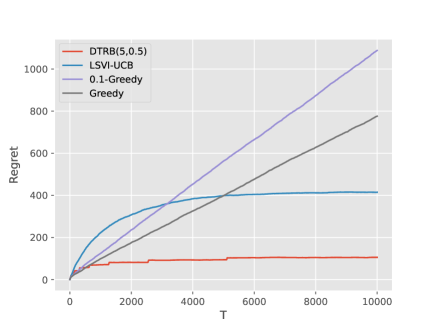
Figure 2: Expected regret of different algorithms.

5.2 Synthetic Experiments

We start by considering a synthetic experiment where we generate data from a model that conforms to our linear $Q$ assumption. We let $\mathbf{X}_{t,1}$ be i.i.d samples from $\text{Uniform}(0,1)$. The second-stage contexts are generated from the following distributions:

$$\mathbb{P}\left(\mathbf{X}_{t,2}(1)=\textbf{x}_{2}\mid\mathbf{X}_{t,1}=\textbf{x}_{1}\right)=\textbf{x}_{1}\text{Beta}_{4,1}(\textbf{x}_{2})+(1-\textbf{x}_{1})\text{Beta}_{1,2}(\textbf{x}_{2}),$$

$$\mathbb{P}\left(\mathbf{X}_{t,2}(2)=\textbf{x}_{2}\mid\mathbf{X}_{t,1}=\textbf{x}_{1}\right)=\textbf{x}_{1}\text{Beta}_{1,4}(\textbf{x}_{2})+(1-\textbf{x}_{1})\text{Beta}_{2,1}(\textbf{x}_{2}).$$

Lastly, $\mathbf{X}_{t,3}(a_{1},1)=\mathbf{X}_{t,2}(a_{1})+1+\epsilon_{t}^{(a_{1},1)}$, and $\mathbf{X}_{t,3}(a_{1},2)=3\mathbf{X}_{t,2}(a_{1})+\epsilon_{t}^{(a_{1},2)}$, where each $\epsilon_{t}^{(a_{1},a_{2})}$ is i.i.d. from $\text{Normal}(0,1)$. The final reward $Y(a_{1},a_{2})$ equals $\mathbf{X}_{t,3}(a_{1},a_{2})$. With these distributions, we can compute the $Q$-functions in closed form, and the corresponding optimal decision rule is: in the first stage, pull arm $1$ when $\mathbf{X}_{1}>5/14$ and arm $2$ otherwise; in the second stage, pull arm $1$ when $\mathbf{X}_{2}<1/2$ and arm $2$ otherwise. It is easy to check that our example satisfy the conditions in Lemma 1, so it satisfies Assumption 2 with $\alpha=1$.

Fig. 2 shows the regret for different algorithms in this setting. Here we simulate $40$ independent paths up to $T=10{,}000$, and compute the average regret of different algorithms over these paths. Both Greedy and $\epsilon$-Greedy achieve linear regret in the long run, but for different reasons. Greedy suffers from a constant fraction of “bad" paths where the decision-maker stops exploring and repeatedly makes the suboptimal decision from early on due to lack of exploration. On the other hand, $\epsilon$-Greedy suffers from excessive exploration: randomizing with $\epsilon$ probability at each time step means it chooses the sub-optimal arm with $\Omega(\epsilon)$ probability at each time step, which accumulates to $\Omega(\epsilon T)$ regret. LSVI-UCB achieves sub-linear regret, but performs significantly worse than DTRBandit. In contrast to these three, DTRBandit performs very well in the long run and has logarithmic regret.

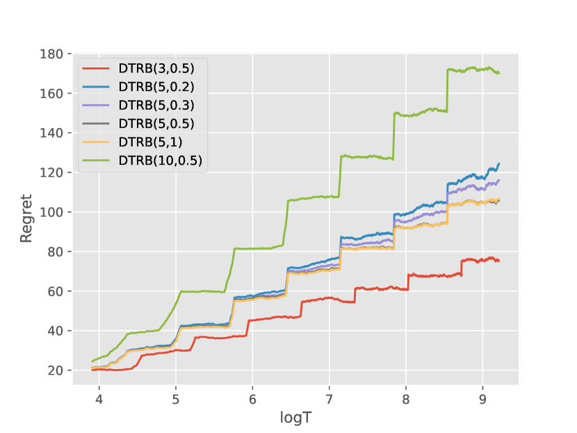
(a) Regret versus $\log T$.

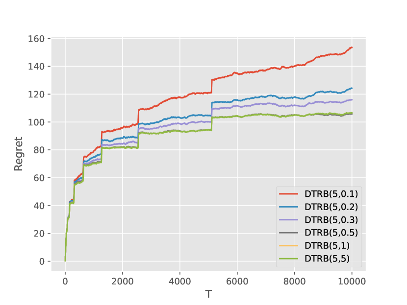
(b) Regret with different $\Delta$’s.

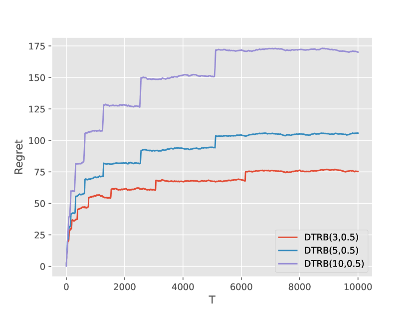
(c) Regret with different $q$’s.

Figure 3: Expected regret of DTRBandit with different $\Delta$ and $q$ inputs.

We now briefly discuss the choice of tuning parameters $\Delta$ and $q$ for DTRBandit. On a high level, larger $q$ means we perform more exploration, and larger $\Delta$ means we rely more on hat-estimators instead of tilde-estimators. Fig. 3 shows the expected regret of DTRBandit with different $\Delta$ and $q$ inputs. First of all, DTRBandit is very robust to the choices of these parameters, and Fig. 3(a) shows that it achieves logarithmic regret across different parameter choices, which agrees with our theoretical results in Section 4. It is interesting to see that we can achieve logarithmic regret in practice even when $q$ is much smaller than what would be theoretically required by Theorem 1, and $\Delta$ is much larger than what would be theoretically required to satisfy Assumption 3. Moreover, the cumulative regret gets lower as $q$ gets smaller, and $\Delta$ gets larger. Therefore, in practice, we suggest following a “small $q$, large $\Delta$ (compared to the scale of rewards)" rule-of-thumb to choose these parameters.

5.3 Empirical Study: STAR*D Data

We next study the algorithms using real data, where our linear $Q$ assumption likely does not hold.

5.3.1 Background on STAR*D and Problem Formulation.

Sequenced Treatment Alternatives to Relieve Depression (STAR*D) was a multi-level randomized controlled trial designed to assess effectiveness of different treatment regimes for patients with major depressive disorder (Rush et al. 2004). The primary outcome at each level (i.e., stage) was assessed using the QIDS scores, which measures severity of depression and ranges from $0$ to $26$ in the sample. Before each treatment level, participants with a total clinican-rated QIDS-score of $0$ to $5$ were considered as having a clinically meaningful response and therefore in remission, and those without remission were eligible for future treatments and entered the next treatment level.

Following existing literature (Chakraborty et al. 2013, Liu et al. 2018), we focus on level $2/2A$ (referred to as stage $1$) and level $3$ (referred to as stage $2$) of the study only. There were $1260$ participants with complete features who entered stage $1$; $468$ of them achieved remission, $465$ of them dropped out, and $327$ of them entered stage $2$. The treatments were divided into two groups: one group that involves SSRIs (selective serotonin reuptake inhibitors), and the other that involves only non-SSRIs.

We define the following context, treatment, and outcome variables:

• $\mathbf{X}_{1}$: QIDS-score measured at the start of stage $1$ (QIDS.start₁), the slope of QIDS-score over the previous level (QIDS.slope₁), and participant preference at the start of stage $1$ (preference₁, taking values $1,2$). We let $\psi_{1}(\mathbf{H}_{1})=\mathbf{X}_{1}$.

• $A_{1}$: $1$ if treated with SSRI drugs in stage $1$, and $2$ if treated with non-SSRI drugs.

• $\mathbf{X}_{2}$: QIDS.end₁ measured at the start of stage $1$, QIDS.start₂, QIDS.slope₂ and preference₂ measured at the start of stage $2$. We let $\psi_{2}(\mathbf{H}_{2})=(\text{QIDS.start}_{2},\text{QIDS.slope}_{2}$, $\text{preference}_{2})$.

• $A_{2}$: $1$ if treated with SSRI drugs in stage $2$, $2$ if treated with non-SSRI drugs. In the dataset, if a patient is treated with a non-SSRI drug in stage $1$, then $A_{2}\equiv 2$.

• $\mathbf{X}_{3}$: QIDS.end₂ measured at the start of stage $2$.

• $Y$: Let $R=1$ if the patient achieves remission before stage $2$, and $0$ otherwise. Define

  $$Y=-R\cdot\text{QIDS.end}_{1}-(1-R)\cdot\left(\frac{\text{QIDS.end}_{1}+\text{QIDS.end}_{2}}{2}\right).$$

  Here we take the negative of QIDS-scores to make higher values correspond to better outcomes.

The STAR*D dataset is then viewed as 1260 observations of the above variables, one for each participant with complete features who entered stage 1. However, in contrast to existing literature that focuses on offline DTR estimation and evaluation methods, we aim to learn a mapping between patient covariates and the optimal treatment regime in a online and adaptive manner. Therefore, we do not simply observe all data points at once nor do we even observe all of them sequentially. We next discuss how we use this data to nonetheless evaluate online DTR bandit algorithms.

5.3.2 Off-policy DTR Bandit Algorithm Evaluation

For any given DTR bandit algorithm $\mathcal{A}$, we want to evaluate its performance using the average reward it collects up to each fixed time $T$, i.e.,

$${g}_{T}(\mathcal{A})=\mathbb{E}\left[\frac{1}{T}\sum_{t=1}^{T}Y_{t}(A_{t,1},A_{t,2})\right],$$

where $A_{t,1}$ and $A_{t,2}$ are obtained by running algorithm $\mathcal{A}$. Because we only have access to outcomes of the treatments administered in the STAR*D dataset and never for treatments not administered, estimating ${g}_{T}(\mathcal{A})$ using this dataset is nontrivial. This is known as off-policy evaluation.

Our key idea for off-policy DTR bandit algorithm evaluation stems from the Policy-Evaluator Algorithm (Li et al. 2011, Algorithm $1$), which gives an unbiased estimator of the average reward for contextual bandit algorithms. Assume that $S$ is a dataset obtained from a uniformly randomized sequential trial, i.e., $(a_{1},a_{2})$ are chosen uniformly at random to generate the data. Then we could evaluate a DTR bandit algorithm $\mathcal{A}$ as follows. We play through the data sequentially. First we set $t=0$. For each data point $(\textbf{x}_{1},a_{1},\textbf{x}_{2},a_{2},\textbf{x}_{3},y)$ in $S$, we first show $\textbf{x}_{1}$ to $\mathcal{A}$. If it takes an action different from $a_{1}$ in the first stage, we skip this data point, ignoring the outcomes, not adding it to our history, and not increasing the time counter $t$. Otherwise, we additionally show $(a_{1},\textbf{x}_{2})$ to $\mathcal{A}$. Again, if it takes an action different from $a_{2}$ in the second stage, we skip this data point. Otherwise, if it matched both $a_{1}$ and $a_{2}$, we add the outcome (divided by $T$) to our cumulative reward, add the data point to our history, and increment $t$. We repeat this procedure until we get $T$ samples in our trajectory. In the end, we must have an unbiased estimator for ${g}_{T}(\mathcal{A})$.

Algorithm 2 ReplayDTR

1:  Inputs: $T>0$; online DTR algorithm $\mathcal{A}$; dataset $S$; weights $\{1/p_{i}\}_{i\in S}$.

2:  $\text{hist}_{0}\leftarrow()$  {An initially empty history}

3:  $\hat{G}(\mathcal{A})\leftarrow 0$  {An initially zero total payoff}

4:  for $t=1,2,\dots,T$ do

5:     repeat

6:      Sample the next data point $(\mathbf{x}_{1},a_{1},\mathbf{x}_{2},a_{2},\mathbf{x}_{3},y)$ according to weights $\{1/p_{i}\}_{i\in S}$ from $S$ with replacement

7:     until $\mathcal{A}(\text{hist}_{t-1},\mathbf{x}_{1})=a_{1},\,\mathcal{A}(\text{hist}_{t-1},\mathbf{x}_{1},a_{1},\mathbf{x}_{2})=a_{2}$

8:     $\text{hist}_{t}\leftarrow(\text{hist}_{t-1},\mathbf{x}_{1},a_{1},\mathbf{x}_{2},a_{2},\mathbf{x}_{3},y)$

9:     $\hat{G}(\mathcal{A})\leftarrow\hat{G}(\mathcal{A})+y$

10:  end for

10:  Output: $\hat{G}(\mathcal{A})/T$

However, the STAR*D data does not come from a uniformly randomized trial and the randomization probabilities are adapted to each participant’s time-varying features (but not adapted over participants). Moreover, since we are evaluating a history-dependent online algorithm rather than a fixed policy, we cannot simply reweight the outcomes in the average reward computed from the previously mentioned method. We tackle this problem by using weighted sampling from STAR*D data (with replacement), so that each data point looks like coming from uniform randomization between arms. Specifically, first, we estimate the propensity $p_{i}$ of the $i$-th point $(\textbf{x}_{1i},a_{1i},\textbf{x}_{2i},a_{2i},\textbf{x}_{3i},y_{i})$ in STAR*D, i.e., the probability we choose $(a_{1i},a_{2i})$ given the features. $p_{i}$ is estimated as the product of three parts: i) the probability of choosing $a_{1i}$ in stage $1$ (from a logistic model using $\textbf{x}_{1i}$ as predictors), ii) the probability of stay/drop-out in stage $2$ (from a logistic model using $\textbf{x}_{1i}$, $a_{1i}$, $\textbf{x}_{1i}a_{1i}$ and QIDS.slope₂ as predictors), and iii) the probability of choosing $a_{i,2}$ in stage $2$ if the $i$-th point is present in stage $2$ (from a logistic model using $\textbf{x}_{1i}$, $a_{1i}$, $\textbf{x}_{1i}a_{1i}$ and $\textbf{x}_{2i}$ as predictors). We then assign weight $1/p_{i}$ to the $i$-th data point, and to generate the next data point $(\mathbf{x}_{1},a_{1},\mathbf{x}_{2},a_{2},\mathbf{x}_{3},y)$, we sample from $S$ according to weights $\{1/p_{i}\}_{i\in S}$ with replacement. The rest of our algorithm is the same as in the uniformly randomized case, and the detailed evaluation procedure is summarized in Algorithm 2.

5.3.3 Comparison of Algorithms

Again, we compare the empirical performance of DTRBandit with Greedy, $\epsilon$-Greedy and LSVI-UCB. In addition, we use the following two as benchmarks for comparison:

1. Logging: the average rewards observed in the STAR*D dataset after adjusting for dropouts (which estimates $g_{T}(\mathcal{A})$ for the logging policy that generated the data).

2. Offline: the average rewards of the estimated optimal treatment regime using the whole offline dataset (given in Chakraborty et al. 2013), which suggests treating a patient in stage $1$ with SSRI if $(-0.73+0.01\times\text{QIDS.start}_{1}+0.01\times\text{QIDS.slope}_{1}-0.67\times\text{preference}_{1})>0$ (and with a non-SSRI otherwise), and treating a patient in stage $2$ with SSRI if $(-0.18-0.01\times\text{QIDS.start}_{2}-0.25\times\text{QIDS.slope}_{2})>0$ (and with a non-SSRI otherwise).

To be consistent with real-world practice, all algorithms are implemented with the extra condition that we do not enter the second stage when $\text{QIDS.end}_{1}\leq 5$, and we can only use non-SSRI drugs in stage $2$ if we use non-SSRI drugs in stage $1$. When implementing DTRBandit and $\epsilon$-Greedy, because when $\text{QIDS.end}_{1}\leq 5$, the outcome $Y$ is determined by the observations before stage $2$, we define $\tilde{Y}=\hat{Y}=\text{QIDS.end}_{1}$ for data points with $\text{QIDS.end}_{1}\leq 5$; we attempted a similar change when implementing LSVI-UCB, but its performance gets worse, so we do not make this change for LSVI-UCB. Besides, for all algorithms, in both defining and estimating $Q_{1}(\textbf{h},2)$, we replace the max with the estimated value of pulling arm $2$ in stage $2$, because arm $2$ is the only feasible arm afterwards. Our exploration schedule for DTRBandit is updated to explore the $3$ first- and second-stage treatment combinations that appear in the data, because we do not need to learn about the infeasible treatment plan $(2,1)$. Moreover, since Jin et al. (2019) require the feature map to be bounded by $1$, we normalize the features when running LSVI-UCB. Lastly, for DTRBandit, we vary the margin parameter $\Delta$ and force-pull schedule parameter $q$, while following the general rule of “small $q$, large $\Delta$" as we discussed in Section 5.2. Compared with synthetic experiments, we choose smaller $q$’s since the horizon is shorter, and larger $\Delta$’s since the scale of the final outcome is much larger.

Table 1: Average rewards of different algorithms at $T=5000$

DTRB(1, 10)	DTRB(1, 20)	DTRB(1, 50)	DTRB(2, 10)	DTRB(2, 20)	DTRB(2, 50)
$-7.680$	$-7.561$	$-7.552$	$-7.688$	$-7.604$	$-7.547$
Logging	LSVI-UCB	Greedy	0.1-Greedy	0.2-Greedy	Offline
$-8.438$	$-8.071$	$-7.810$	$-7.724$	$-7.835$	$-7.688$

Table 1 presents the average rewards evaluated at $T=5{,}000$. Here we generated $10$ independent paths from the STAR*D data set, and compute the mean of the average rewards of different algorithms over these paths. All online algorithms improve substantially from the logging policy used in the original dataset. In particular, DTRBandit consistently performs well under different parameter choices, achieves the highest average reward among all online algorithms, and is often better than the Offline benchmark that roughly serves as a proxy for “good algorithms". Interestingly, we find that the performance of DTRBandit gets better when $q$ gets smaller and $\Delta$ gets larger. This is consistent with our discovery in Section 5.2, and can serve as a general guideline for choosing these parameters in practice.

6 Conclusions and Future Directions

In this paper, we define and solve the DTR bandit problem, where we can both personalize initial decision to each incoming unit and adapt a second-linear decision after observing the effect of the first-line decision. We propose a novel algorithm that achieves rate-optimal regret under the linear $Q$ model. Our algorithm shows favorable empirical performance in both synthetic scenarios and in a real-world healthcare dataset.

We discuss several extensions of work, some of which we will detail in the appendix. In Appendix C, we extend our model to the setting where the feedback from second-stage outcomes may be delayed until after a new unit already arrives. We provide a revised algorithm for a large class of arrival processes, and show that the additional regret due to delays is additive. In Appendix D, we discuss the extension to two-stage DTR bandits with more than two arms, where we also allow for the possibility of arms that are everywhere suboptimal, in violation of Assumption 3. We extend our analysis to show that a slightly modified algorithm has the same order of regret as in Theorem 1. Finally, the extension to $M>2$ stages is straightforward. For each intermediate stage $m\in[M-1]$, we can compute $\tilde{Y}_{m,j}=\max_{a\in[2]}\tilde{\boldsymbol{\beta}}_{a,m+1}^{\intercal}(t)\boldsymbol{\psi}_{m+1}(\mathbf{H}_{j,m+1})$ and $\hat{Y}_{m,j}=\max_{a\in[2]}\hat{\boldsymbol{\beta}}_{a,m+1}^{\intercal}(t)\boldsymbol{\psi}_{m+1}(\mathbf{H}_{j,m+1})$. The corresponding $\tilde{\boldsymbol{\beta}}_{a,m}(t)$ and $\hat{\boldsymbol{\beta}}_{a,m}(t)$ can be obtained by regressing $\tilde{Y}_{m,j}$ and $\hat{Y}_{m,j}$ on $\boldsymbol{\psi}_{m}(\mathbf{H}_{j,m})$. The rest of the algorithm can be extended by changing $m\in[2]$ to $m\in[M]$.

Appendices

Appendix A Regret Upper Bound Analysis

In this section, we provide an outline for the analysis of the regret upper bound. Here we break up our analysis into modular Propositions, each of which we prove in detail in Appendix B, and then we explain how these results come together to establish Theorem 1.

A.1 OLS Tail Inequality for Adaptive Observations with Measurement Error.

The key to get uniform (over $\mathcal{H}_{1}$ or $\mathcal{H}_{2}$) concentration bounds on the estimated $Q$-functions is to get good concentration bounds for the OLS estimators $\tilde{\boldsymbol{\beta}}_{a,m},\hat{\boldsymbol{\beta}}_{a,m}$. However, in our bandit setup, the observations from pulling a certain arm are not independent. Moreover, the true outcome $\max_{a_{2}\in[2]}Q_{2}\left(\mathbf{H}_{t,2}(a_{1}),a_{2}\right)$ is not observable in practice, and we can only run OLS on an imputed value with some possible measurement error. In this section, we provide a general result for OLS estimators from adaptive samples with measurement error, which will be frequently utilized in later sections.

Proposition 2 (OLS Tail Inequality for Adaptive Observations with Measurement Error).

Let $S=\{(\mathbf{H}_{i},Y_{i})\}_{i=1}^{n}$ be samples generated from a linear model $Y_{i}=\boldsymbol{\beta}^{T}\mathbf{g}(\mathbf{H}_{i})+\epsilon_{i}+\delta_{i}$ with unknown $\boldsymbol{\beta}\in\mathbb{R}^{d}$ and known $\mathbf{g}:\mathcal{H}\rightarrow\mathbb{R}^{d}$. Assume that there exists a filtration $\{\mathcal{F}_{i}\}_{i=0}^{n}$ such that $\{g_{j}(\mathbf{H}_{i})\epsilon_{i}\}_{i=1}^{n}$ is a martingale difference sequence adapted to the filtration, where $g_{j}(\mathbf{H}_{i})$ denotes the $j$-th entry of $\mathbf{g}(\mathbf{H}_{i})$. If $||\mathbf{g}(\mathbf{H}_{i})||\leq x_{\max}$, $||\mathbf{g}(\mathbf{H}_{i})||_{\infty}\leq x_{\infty}$ and $\epsilon_{i}$ is $\sigma$-sub-Gaussian for all $i\in[n]$ in an adaptive sense, the following tail inequality holds for all $\chi>0$ and $\phi>0$:

$$\mathbb{P}\left(\left\lVert\hat{\boldsymbol{\beta}}-\boldsymbol{\beta}\right\rVert\geq\chi,\lambda_{\min}\left(\hat{\Sigma}\right)\geq\phi\right)\leq 2d\exp\left(-\frac{\chi^{2}\phi^{2}}{8ndx_{\infty}^{2}\sigma^{2}}\right)+\mathbb{P}\left(\sum_{i=1}^{n}\left|\delta_{i}\right|\geq\frac{\chi\phi}{2x_{\max}}\right),$$

where $\hat{\Sigma}=\sum_{i=1}^{n}\mathbf{g}(\mathbf{H}_{i})\mathbf{g}^{\intercal}(\mathbf{H}_{i})$ and $\hat{\boldsymbol{\beta}}=\hat{\Sigma}^{-1}\left(\sum_{i=1}^{n}\mathbf{g}(\mathbf{H}_{i})Y_{i}\right)$.

A.2 Concentration of the Forced-Pull Estimators.

We are now equipped to prove the convergence of our forced-pull estimators. Define $\mathcal{G}_{t,m}$ to be the event that our $\tilde{Q}_{t,m}$ has good estimation accuracy uniformly over both arms and all $\textbf{h}\in\mathcal{H}_{m}$:

$$\mathcal{G}_{t,m}\triangleq\left\{\max_{a\in[2]}\sup_{\textbf{h}\in\mathcal{H}_{m}}|\tilde{Q}_{t,m}(\textbf{h},a)-Q_{m}(\textbf{h},a)|\leq\frac{\Delta_{m}}{4}\right\},\quad t\in[T],m\in[2],$$ (12)

and $\mathcal{G}_{t}$ to be the event that both $\mathcal{G}_{t,1}$ and $\mathcal{G}_{t,2}$ hold at time $t$:

$$\mathcal{G}_{t}\triangleq\mathcal{G}_{t,1}\cap\mathcal{G}_{t,2}.$$

The following proposition shows that both $\mathcal{G}_{t,1}$ and $\mathcal{G}_{t,2}$ (thus, also $\mathcal{G}_{t}$) hold with high probability.

Proposition 3.

When $q\geq\tilde{C}_{1}\vee\tilde{C}_{2}$ and $t\geq 64q^{2}$,

1. $\mathbb{P}(\mathcal{G}_{t,1})\geq 1-\frac{{8}}{t^{2}},$

2. $\mathbb{P}(\mathcal{G}_{t,2})\geq 1-\frac{{6}}{t^{2}}.$

To prove Proposition 3, we note that by the construction of forced sampling, $\{(\mathbf{H}_{j,2},Y_{j}):j\in\mathcal{T}_{a,2}(t)\}$ is a set of independent samples. Therefore, we can use Proposition 2 to get concentration bounds for $\tilde{\boldsymbol{\beta}}_{a,2}(t)$. When $\tilde{\boldsymbol{\beta}}_{a,2}(t)$ is well-concentrated, $\tilde{Y}_{j}$ is close enough to $\max_{a\in[2]}\boldsymbol{\beta}^{\intercal}_{a,2}\boldsymbol{\psi}_{2}(\mathbf{H}_{j,2})$, so applying Proposition 2 again we get concentration bounds for $\tilde{\boldsymbol{\beta}}_{a,1}(t)$. The only missing part is the positive-definiteness of the design matrices. Because $\{\mathbf{H}_{j,m}:j\in\mathcal{T}_{a,m}(t)\}$ are independent samples, by the matrix Chernoff inequality (see, e.g., Tropp, 2015, Theorem 5.1.1), the minimal eigenvalue of the corresponding design matrix concentrates around the minimal eigenvalue of its mean. Assumption 3 guarantees that the latter is strictly positive, thus our design matrix has lower-bounded minimal eigenvalue with high probability (Lemmas 4 and 5). Proposition 3 then follows naturally.

A.3 Concentration of the All-Samples Estimators.

Next, we consider tail bounds on the all-samples estimators. Define $\mathcal{M}_{t,m}$ to be the event that the minimum eigenvalues of both $\hat{\Sigma}_{1,m}(t)$ and $\hat{\Sigma}_{2,m}(t)$ grow at least linearly in $t$:

$$\mathcal{M}_{t,m}=\left\{\lambda_{\min}\left(\hat{\Sigma}_{1,m}(t)\right)\geq\frac{\phi_{m}t}{4}\right\}\cap\left\{\lambda_{\min}\left(\hat{\Sigma}_{2,m}(t)\right)\geq\frac{\phi_{m}t}{4}\right\},$$ (13)

For notation brevity, we let $\mathcal{M}_{t}=\mathcal{M}_{t,1}\cap\mathcal{M}_{t,2}$. Consider the samples $\left\{\left(\mathbf{H}_{j,2},Y_{j}\right)\right\}_{j\in\mathcal{S}_{a,2}(t)}$. Let $\mathcal{F}_{j}$ be the $\sigma$-algebra generated by $\left\{\mathbf{H}_{i,2},A_{i,2},Y_{i}\right\}_{i\in[j]}\cup\mathbf{H}_{j+1,2}$. If we denote the $k$-th entry of $\boldsymbol{\psi}_{2}\left(\mathbf{H}_{j,2}\right)$ as $\boldsymbol{\psi}_{2k}\left(\mathbf{H}_{j,2}\right)$, it is easy to see that $\left\{\boldsymbol{\psi}_{2k}(\mathbf{H}_{j,2})\eta_{j,2}^{(A_{j,1},a)}\mathbb{I}\left\{A_{j,2}=a\right\}\right\}_{j=1}^{T}$ is a martingale difference sequence adapted to $\left\{\mathcal{F}_{j}\right\}_{j=1}^{T}$. Therefore, we can use similar arguments as in the proof of Proposition 2 to get tail bounds on $\hat{\boldsymbol{\beta}}_{a,1}(t)$ under the event $\mathcal{M}_{t}$. Moreover, we can apply similar arguments to $\left\{\left(\mathbf{H}_{j,1},\hat{Y}_{j}\right)\right\}_{j\in\mathcal{S}_{a,2}(t)}$ to get a concentration bound on $\hat{\boldsymbol{\beta}}_{a,2}(t)$ under $\mathcal{M}_{t}$. Combining all these parts together we get the following two results:

Proposition 4.

For any $t\in[T]$,

$$\mathbb{P}\left(\max_{\textbf{h}\in\mathcal{H}_{1}}\left|\hat{Q}_{t,1}(\textbf{h},a)-Q_{1}(\textbf{h},a)\right|>\chi,\mathcal{M}_{t}\right)\leq 2d\exp\left(-\frac{\phi_{1}^{2}\chi^{2}t}{128dx_{\infty}^{2}x_{\max}^{2}\sigma^{2}}\right)+4d\exp\left(-\frac{\phi_{1}^{2}\phi_{2}^{2}\chi^{2}t}{2048dx_{\infty}^{2}x_{\max}^{6}\sigma^{2}}\right).$$

Proposition 5.

For any $t\in[T]$,

$$\mathbb{P}\left(\max_{x\in\mathcal{X}_{1}}|\hat{Q}_{t,2}(x,a)-Q_{2}(x,a)|>\chi,\mathcal{M}_{t}\right)\leq 2d\exp\left(-\frac{\phi_{2}^{2}\chi^{2}t}{32dx_{\max}^{2}x_{\infty}^{2}\sigma^{2}}\right).$$

What remains is to prove that $\mathcal{M}_{t}^{C}$ happens with low probability. Consider the following subsets of $\mathcal{S}_{a,m}$:

$$\mathcal{S}_{a,1}^{\prime}(t)=\left\{j\in[t]:j\not\in\cup_{a_{1},a_{2}\in[2]}\mathcal{T}_{(a_{1},a_{2})},\mathbf{H}_{j,1}\in U_{a,1},\mathcal{G}_{j-1,1}\right\},$$ (14)

$$\mathcal{S}^{\prime}_{a,2}(t)=\bigcup_{i\in[2]}\left\{j\in[t]:j\not\in\cup_{a_{1},a_{2}\in[2]}\mathcal{T}_{(a_{1},a_{2})},\mathbf{H}_{j,1}\in U_{i,1},\mathbf{H}_{j,2}(i)\in U_{a,2},\mathcal{G}_{j-1}\right\}.$$ (15)

Lemma 7 shows that $\left\{\mathbf{H}_{j,m}:j\in\mathcal{S}_{a,m}^{\prime}(t)\right\}$ are independent samples. We can then prove that under Assumption 3, $\left|\mathcal{S}_{a,m}^{\prime}(t)\right|<p_{m}t/4$ happens with low probability. Moreover, we can apply the matrix Chernoff inequality to show that $\lambda_{\min}\left(\sum_{s\in\mathcal{S}^{\prime}_{a,m}(t)}\mathbf{H}_{s,m}\mathbf{H}_{s,m}^{\intercal}\right)$ concentrates around the smallest eigenvalue of the mean of $\sum_{s\in\mathcal{S}^{\prime}_{a,m}(t)}\mathbf{H}_{s,m}\mathbf{H}_{s,m}^{T}$, which grows linearly when $\left|\mathcal{S}_{a,m}^{\prime}(t)\right|=\Omega(t)$. Using the trivial relationship that $\lambda_{\min}\left(\hat{\Sigma}_{a,m}(t)\right)\geq\lambda_{\min}\left(\sum_{s\in\mathcal{S}^{\prime}_{a,m}(t)}\mathbf{H}_{s,m}\mathbf{H}_{s,m}^{\intercal}\right)$, since all summand matrices are positive semidefinite, we can get the following bound on $\mathbb{P}(\mathcal{M}_{t}^{C})$:

Proposition 6.

When $q\geq\tilde{C}_{1}\vee\tilde{C}_{2}$, $t\geq 256q^{2}$ and $t\in\left(\cap_{a_{1},a_{2}\in[2]}\mathcal{T}_{(a_{1},a_{2})}^{C}\right)\cup\{2^{j}q\}_{j\geq 5}$ (i.e., when we do not force-pull, or when we are at the last step of a force-pull stage),

$$\mathbb{P}\left(\mathcal{M}_{t}^{C}\right)\leq\sum_{m\in[2]}2d\exp\left(-\frac{\phi_{m}t}{48x_{\max}^{2}}\right)+\frac{280}{t^{2}}.$$

A.4 Regret Upper Bound

Finally, we can compute the upper bound on our algorithm’s regret. Define $\mathcal{T}_{0}=\left\{t:t\leq 256q^{2}\right\}\cup\mathcal{T}_{1,1}\cup\mathcal{T}_{2,1}$. We then decompose the regret of our algorithm into four exhaustive cases:

1. $R^{(1)}$: when we initialize or explore ($t\in\mathcal{T}_{0}$);

2. $R^{(2)}$: when $t\not\in\mathcal{T}_{0}$, and $\mathcal{G}_{t-1}\cap\mathcal{M}_{t-1}$ does not hold;

3. $R^{(3)}$: when $t\not\in\mathcal{T}_{0}$, $\mathcal{G}_{t-1}\cap\mathcal{M}_{t-1}$ holds, and we pull the suboptimal arm in the first stage;

4. $R^{(4)}$: when $t\not\in\mathcal{T}_{0}$, $\mathcal{G}_{t-1}\cap\mathcal{M}_{t-1}$ holds, and we pull the suboptimal arm in the second stage.

Our regret is the sum of these four terms. To analyze our regret, we next show how control each of the terms, $R^{(1)}$ to $R^{(4)}$.

First, note that the per-step regret is always bounded by $6b_{\max}x_{\max}$. Because we have at most $3q\log t$ forced pulls on each arm up to time $t$ when $t\geq 64q^{2}$ (Lemma 3), it is easy to see that $R^{(1)}\leq 8qb_{\max}x_{\max}(3\log T+128q)$.

Next, Propositions 3 and 6 guarantee that $\mathbb{P}\left(\mathcal{G}_{t}^{C}\cup\mathcal{M}_{t}^{C}\right)$ is of order $O(1/t^{2})$, so summing up over $t\not\in\mathcal{T}_{0}$ we get $R^{(2)}\leq 24b_{\max}x_{\max}\left(49+16dx_{\max}^{2}/\phi_{1}+16dx_{\max}^{2}/\phi_{2}\right)$.

Thirdly, when $\mathcal{G}_{t-1}\cap\mathcal{M}_{t-1}$ holds, we never make a mistake when we use only the $\tilde{Q}$ estimators to make a decision, so regret comes only when the $\tilde{Q}$ estimators are close and we use $\hat{Q}$ estimators to make decisions. When $\mathbf{H}_{t,1}$ falls into the region where $|Q_{1}(\mathbf{H}_{t,1},1)-Q_{1}(\mathbf{H}_{t,1},2)|=O\left(t^{-1/2}\right)$, our algorithm may pull the suboptimal arm. However, such event happens with low probability $O(t^{-\alpha_{1}/2})$ by Assumption 2, and the regret we incur in such an event is of order $O(t^{-1/2})$, so the total regret caused by such event is controllable. On the other hand, when $\mathbf{H}_{t,1}$ falls into the region where $|Q_{1}(\mathbf{H}_{t,1},1)-Q_{1}(\mathbf{H}_{t,1},2)|=\Omega\left(t^{-1/2}\right)$, by Proposition 4 we very rarely make a mistake and pull the suboptimal arm at time $t$. Therefore, using a peeling argument, we obtain $R^{(3)}\leq 2^{\alpha_{1}+2}\gamma_{1}C_{1}^{-\frac{\alpha_{1}+1}{2}}\left((M+2)^{\alpha_{1}+2}+2^{\alpha_{1}+6}\right)f(\alpha_{1})$.

The analysis of $R^{(4)}$ is almost analogous to the analysis of $R^{(3)}$, and we get $R^{(4)}\leq 2^{\alpha_{2}+3}\gamma_{2}C_{2}^{-\frac{\alpha_{2}+1}{2}}\left((M+2)^{\alpha_{2}+2}+2^{\alpha_{2}+4}\right)f(\alpha_{2})$. Adding all four terms together we get the result in Theorem 1.

Appendix B Omitted Proofs

In this section, any $a$ denotes one of the arms and can take value in $[2]$.

B.1 Proofs in Section 2

Proof of Proposition 1..

On one hand,

$$\mathbb{E}\left[Y_{t}(A^{*}_{t,1},A^{*}_{t,2})\right]= \mathbb{E}\left[Q_{2}(\mathbf{H}^{*}_{t,2},A^{*}_{t,2})\right]$$

$$= \mathbb{E}\left[\max_{a_{2}}Q_{2}(\mathbf{H}^{*}_{t,2},a_{2})\right]$$

$$= \mathbb{E}\left[\mathbb{E}\left[\max_{a_{2}}Q_{2}(\mathbf{H}^{*}_{t,2},a_{2})\mid\mathbf{X}_{t,1},A^{*}_{t,1}\right]\right]$$

$$= \mathbb{E}\left[Q_{1}(\mathbf{X}_{t,1},A^{*}_{t,1})\right].$$

On the other hand,

$$\mathbb{E}\left[Y_{t}(A_{t,1},A_{t,2})\right]= \mathbb{E}\left[Q_{2}(\mathbf{H}_{t,2},A_{t,2}))\right]$$

$$= \mathbb{E}\left[\max_{a_{2}}Q_{2}(\mathbf{H}_{t,2},a_{2})\right]-\mathbb{E}\left[\max_{a_{2}}Q_{2}(\mathbf{H}_{t,2},a_{2})\right]+\mathbb{E}\left[Q_{2}(\mathbf{H}_{t,2},A_{t,2})\right]$$

$$= \mathbb{E}\left[Q_{1}(\mathbf{X}_{t,1},A_{t,1})\right]-\mathbb{E}\left[\max_{a_{2}}Q_{2}(\mathbf{H}_{t,2},a_{2})\right]+\mathbb{E}\left[Q_{2}(\mathbf{H}_{t,2},A_{t,2})\right].$$

Taking a difference between these two we get the desired result. ∎

Proof of Lemma 1.

We will give a detailed proof for $\alpha_{1}=1$. The arguments for $\alpha_{2}=1$ are similar.

For simplicity suppose $\boldsymbol{\beta}_{1,1}\neq\boldsymbol{\beta}_{2,1}$; otherwise pulling either arm is optimal in stage $1$. Letting $V_{d}(R)$ be the volume of the $R$-radius $d$-ball, we have

$$\mathbb{P}\left(0<\left|Q_{1}\left(\mathbf{X}_{t,1},1\right)-Q_{1}\left(\mathbf{X}_{t,1},2\right)\right|\leq\kappa\right)\leq 2\mathbb{P}\left(0<\left(\boldsymbol{\beta}_{1,1}-\boldsymbol{\beta}_{2,1}\right)^{\intercal}\boldsymbol{\psi}_{1}\left(\mathbf{X}_{t,1}\right)\leq\kappa\right)$$

$$\leq 2\mu_{\max}\int_{0}^{\kappa/\left\lVert\boldsymbol{\beta}_{1,1}-\boldsymbol{\beta}_{2,1}\right\rVert}V_{d-1}\left(\left(x_{\max}^{2}-u^{2}\right)_{+}^{1/2}\right)du$$

$$\leq 12\mu_{\max}x_{\max}^{d}\kappa/\left\lVert\boldsymbol{\beta}_{1,1}-\boldsymbol{\beta}_{2,1}\right\rVert.$$

∎

B.2 Proofs for Regret Upper Bound

B.2.1 Proofs in Section A.1

Proof of Proposition 2..

It is easy to check that $\hat{\boldsymbol{\beta}}-\boldsymbol{\beta}=\hat{\Sigma}^{-1}\left(\sum_{i=1}^{n}g(\mathbf{H}_{i})\epsilon_{i}+\sum_{i=1}^{n}g(\mathbf{H}_{i})\delta_{i}\right)$. When the event $\lambda_{\min}\left(\hat{\Sigma}\right)\geq\phi$ holds,

$$\left\lVert\hat{\boldsymbol{\beta}}-\boldsymbol{\beta}\right\rVert =\left\lVert\hat{\Sigma}^{-1}\left(\sum_{i=1}^{n}g(\mathbf{H}_{i})\epsilon_{i}+\sum_{i=1}^{n}g(\mathbf{H}_{i})\delta_{i}\right)\right\rVert$$

$$\leq\left\lVert\hat{\Sigma}^{-1}\right\rVert\cdot\left(\left\lVert\sum_{i=1}^{n}g(\mathbf{H}_{i})\epsilon_{i}\right\rVert+\left\lVert\sum_{i=1}^{n}g(\mathbf{H}_{i})\delta_{i}\right\rVert\right)$$

$$\leq\frac{1}{\phi}\left\lVert\sum_{i=1}^{n}g(\mathbf{H}_{i})\epsilon_{i}\right\rVert+\frac{1}{\phi}\left\lVert\sum_{i=1}^{n}g(\mathbf{H}_{i})\delta_{i}\right\rVert$$

$$\leq\frac{1}{\phi}\left\lVert\sum_{i=1}^{n}g(\mathbf{H}_{i})\epsilon_{i}\right\rVert+\frac{x_{\max}}{\phi}\sum_{i=1}^{n}\left|\delta_{i}\right|.$$

Therefore, for any $\chi>0$,

$$\mathbb{P}\left(\left\lVert\hat{\boldsymbol{\beta}}-\boldsymbol{\beta}\right\rVert\geq\chi,\lambda_{\min}\left(\hat{\Sigma}\right)\geq\phi\right)\leq\mathbb{P}\left(\left\lVert\sum_{i=1}^{n}g(\mathbf{H}_{i})\epsilon_{i}\right\rVert\geq\frac{\chi\phi}{2}\right)+\mathbb{P}\left(\sum_{i=1}^{n}\left|\delta_{i}\right|\geq\frac{\chi\phi}{2x_{\max}}\right).$$

Note that

$$\mathbb{P}\left(\left\lVert\sum_{i=1}^{n}g(\mathbf{H}_{i})\epsilon_{i}\right\rVert\geq\frac{\chi\phi}{2}\right)\leq\sum_{j=1}^{d}\mathbb{P}\left(\left|\sum_{i=1}^{n}g_{j}(\mathbf{H}_{i})\epsilon_{i}\right|\geq\frac{\chi\phi}{2\sqrt{d}}\right).$$

Because each $g_{j}(\mathbf{H}_{i})\epsilon_{i}$ is $x_{\infty}\sigma$-sub-Gaussian and $\{g_{j}(\mathbf{H}_{i})\epsilon_{i}\}_{i=1}^{n}$ is a martingale difference sequence adapted to the filtration $\{\mathcal{F}_{i}\}_{i=0}^{n}$, by Wainwright [2019, theorem 2.19],

$$\mathbb{P}\left(\left|\sum_{i=1}^{n}g_{j}(\mathbf{H}_{i})\epsilon_{i}\right|\geq\frac{\chi\phi}{2\sqrt{d}}\right)\leq 2\exp\left(-\frac{\chi^{2}\phi^{2}}{8ndx_{\infty}^{2}\sigma^{2}}\right).$$

Combining all above pieces we complete the proof.

∎

B.2.2 Proofs in Section A.2

First, we prove a supporting lemma on that bounds the number of forced pulls. Its proof is modified from lemma EC.8 in Bastani and Bayati [2020].

Lemma 3.

If $t\geq 64q^{2}$, then $q\log t\leq|\mathcal{T}_{a,m}(t)|\leq 3q\log t$.

Proof of Lemma 3.

Define the $n$-th consecutive round of forced pulls as

$$L_{n}=\left\{\left(2^{n+2}-4\right)q+1,\dots,2^{n+2}q\right\},\quad n\geq 0.$$

By construction, each arm $a$ is sampled $2q$ times in the $m$-th stage during $L_{n}$. Let $n_{t}=\sup\left\{j\in\mathbb{N}:t\geq 2^{j+2}q\right\}$, and we have $2n_{t}q\leq\left|\mathcal{T}_{a,m}(t)\right|\leq 2(n_{t}+1)q$.

To obtain the lower bound, note that $t\leq 2^{n_{t}+3}q$, which implies $n_{t}\geq\log(t/8q)$. For $t\geq 64q^{2}$,

$$\left|\mathcal{T}_{a,m}(t)\right|\geq 2n_{t}q\geq 2q\log\left(t/8q\right)\geq 2q\left(\log t-\log(8q)\right)\geq q\log t.$$

To obtain the upper bound, note that $t\geq 2^{n_{t}+2}q$, which implies $n_{t}\leq\log_{2}(t/4q)$.

$$\left|\mathcal{T}_{a,m}(t)\right|\leq 2\left(n_{t}+1\right)q\leq 2\log_{2}(t/2q)q\leq 3q\log t.$$

∎

I. Positive Definiteness of Design Matrices.

Lemma 4.

For any $t\in[T]$,

$$\mathbb{P}\left(\lambda_{\min}\left(\tilde{\Sigma}_{a,1}(t)\right)\leq\frac{\phi_{1}}{2}\left|\mathcal{T}_{a,1}(t)\right|\right)\leq d\exp\left(-\frac{\left|\mathcal{T}_{a,1}(t)\right|\phi_{1}}{8x_{\max}^{2}}\right).$$

Proof of Lemma 4.

First we have

$$\lambda_{\max}\left(\boldsymbol{\psi}_{1}\left(\mathbf{H}_{j,1}\right)\boldsymbol{\psi}_{1}^{\intercal}\left(\mathbf{H}_{j,1}\right)\right)=\max_{\left\lVert u\right\rVert=1}u^{T}\boldsymbol{\psi}_{1}\left(\mathbf{H}_{j,1}\right)\boldsymbol{\psi}_{1}^{\intercal}\left(\mathbf{H}_{j,1}\right)u\leq x_{\max}^{2}.$$

Moreover,

$$\lambda_{\min}\left(\mathbb{E}\left[\tilde{\Sigma}_{a,1}(t)\right]\right) =\lambda_{\min}\left(\sum_{j\in\mathcal{T}_{a,1}(t)}\mathbb{E}\left[\boldsymbol{\psi}_{1}\left(\mathbf{H}_{j,1}\right)\boldsymbol{\psi}_{1}^{\intercal}\left(\mathbf{H}_{j,1}\right)\right]\right)$$

$$\geq\lambda_{\min}\left(\sum_{j\in\mathcal{T}_{a,1}(t)}\mathbb{E}\left[\boldsymbol{\psi}_{1}\left(\mathbf{H}_{j,1}\right)\boldsymbol{\psi}_{1}^{\intercal}\left(\mathbf{H}_{j,1}\right)\right]\mathbb{I}\left\{\mathbf{H}_{j,1}\in U_{a,1}\right\}\right)$$

$$\geq\sum_{j\in\mathcal{T}_{a,1}(t)}\lambda_{\min}\left(\mathbb{E}\left[\boldsymbol{\psi}_{1}\left(\mathbf{H}_{j,1}\right)\boldsymbol{\psi}_{1}^{\intercal}\left(\mathbf{H}_{j,1}\right)\right]\mathbb{I}\left\{\mathbf{H}_{j,1}\in U_{a,1}\right\}\right)$$

$$\geq\phi_{1}\left|\mathcal{T}_{a,1}(t)\right|.$$

Because $\left\{\boldsymbol{\psi}_{1}\left(\mathbf{H}_{j,1}\right)\boldsymbol{\psi}_{1}^{\intercal}\left(\mathbf{H}_{j,1}\right)\right\}_{j\in\mathcal{T}_{a,1}(t)}$ are independent, by Matrix Chernoff inequality [cf. Tropp, 2015, Theorem 5.1.1],

$$\mathbb{P}\left(\lambda_{\min}\left(\tilde{\Sigma}_{a,1}(t)\right)\leq\frac{\phi_{1}}{2}\left|\mathcal{T}_{a,1}(t)\right|\right)\leq d\exp\left(-\frac{\left|\mathcal{T}_{a,1}(t)\right|\phi_{1}}{8x_{\max}^{2}}\right).$$

∎

Lemma 5.

For any $t\in[T]$,

$$\mathbb{P}\left(\lambda_{\min}\left(\tilde{\Sigma}_{a,2}(t)\right)\leq\frac{\phi_{2}}{4}\left|\mathcal{T}_{a,2}(t)\right|\right)\leq d\exp\left(-\frac{\left|\mathcal{T}_{a,2}(t)\right|\phi_{2}}{{16}x_{\max}^{2}}\right).$$

Proof of Lemma 5.

By the same argument as in Lemma 4, we know $\lambda_{\max}\left(\boldsymbol{\psi}_{2}\left(\mathbf{H}_{j,2}\right)\boldsymbol{\psi}_{2}^{\intercal}\left(\mathbf{H}_{j,2}\right)\right)\leq x_{\max}^{2}$. Note that

$$\tilde{\Sigma}_{a,2}(t)= \sum_{j\in\mathcal{T}_{a,2}(t)}\boldsymbol{\psi}_{2}\left(\mathbf{H}_{j,2}\right)\boldsymbol{\psi}_{2}^{\intercal}\left(\mathbf{H}_{j,2}\right)$$

$$= \sum_{j\in\mathcal{T}_{a,2}(t)\cap\mathcal{T}_{1,1}(t)}\boldsymbol{\psi}_{2}\left(\mathbf{H}_{j,2}(1)\right)\boldsymbol{\psi}_{2}^{\intercal}\left(\mathbf{H}_{j,2}(1)\right)+\boldsymbol{\psi}_{2}\left(\mathbf{H}_{j+2q,2}(2)\right)\boldsymbol{\psi}_{2}^{\intercal}\left(\mathbf{H}_{j+2q,2}(2)\right),$$

where the last equality follows from our forced-pull schedule. Since

$$\lambda_{\min}\left(\sum_{j\in\mathcal{T}_{a,2}(t)\cap\mathcal{T}_{1,1}(t)}\mathbb{E}\left[\boldsymbol{\psi}_{2}\left(\mathbf{H}_{j,2}(1)\right)\boldsymbol{\psi}_{2}^{\intercal}\left(\mathbf{H}_{j,2}(1)\right)+\boldsymbol{\psi}_{2}\left(\mathbf{H}_{j+2q,2}(2)\right)\boldsymbol{\psi}_{2}^{\intercal}\left(\mathbf{H}_{j+2q,2}(2)\right)\right]\right)$$

$$= \lambda_{\min}\left(\sum_{j\in\mathcal{T}_{a,2}(t)\cap\mathcal{T}_{1,1}(t)}\sum_{a_{1}\in[2]}\mathbb{E}\left[\boldsymbol{\psi}_{2}\left(\mathbf{H}_{j,2}(a_{1})\right)\boldsymbol{\psi}_{2}^{\intercal}\left(\mathbf{H}_{j,2}(a_{1})\right)\right]\right)$$

$$\geq \sum_{j\in\mathcal{T}_{a,2}(t)\cap\mathcal{T}_{1,1}(t)}\lambda_{\min}\left(\sum_{a_{1}\in[2]}\mathbb{E}\left[\boldsymbol{\psi}_{2}\left(\mathbf{H}_{j,2}(a_{1})\right)\boldsymbol{\psi}_{2}^{\intercal}\left(\mathbf{H}_{j,2}(a_{1})\right)\right]\right)$$

$$\geq \frac{\phi_{2}}{2}\left|\mathcal{T}_{a,2}(t)\right|,$$

and each term in the sum is independent, by Matrix Chernoff inequality,

$$\mathbb{P}\left(\lambda_{\min}\left(\tilde{\Sigma}_{a,2}(t)\right)\leq\frac{\phi_{2}}{4}\left|\mathcal{T}_{a,2}(t)\right|\right)\leq d\exp\left(-\frac{\left|\mathcal{T}_{a,2}(t)\right|\phi_{2}}{16x_{\max}^{2}}\right).$$

∎

II. Concentration of $\tilde{Q}_{t,1}$ and $\tilde{Q}_{t,2}$.

Proof of Proposition 3..

First of all, for any $\chi>0$,

$$\mathbb{P}\left(\left\lVert\tilde{\boldsymbol{\beta}}_{a_{2},2}(t)-\boldsymbol{\beta}_{a_{2},2}\right\rVert\geq\chi\right)$$

$$\leq \mathbb{P}\left(\left\lVert\tilde{\boldsymbol{\beta}}_{a_{2},2}(t)-\boldsymbol{\beta}_{a_{2},2}\right\rVert\geq\chi,\lambda_{\min}\left(\tilde{\Sigma}_{a_{2},2}(t)\right)\geq\frac{\phi_{2}}{4}\left|\mathcal{T}_{a_{2},2}(t)\right|\right)+d\exp\left(-\frac{\left|\mathcal{T}_{a_{2},2}(t)\right|\phi_{2}}{16x_{\max}^{2}}\right)$$

$$\leq 2d\exp\left(-\frac{\chi^{2}\phi_{2}^{2}\left|\mathcal{T}_{a_{2},2}(t)\right|}{128dx_{\infty}^{2}\sigma^{2}}\right)+d\exp\left(-\frac{\left|\mathcal{T}_{a_{2},2}(t)\right|\phi_{2}}{16x_{\max}^{2}}\right),$$ (16)

where the first inequality follows from Lemma 5, and the second inequality follows from Proposition 2. Statement 2 is a direct consequence of this result:

$$\mathbb{P}\left(\max_{a_{2}\in[2]}\sup_{\textbf{h}\in\mathcal{H}_{2}}\left|\tilde{Q}_{t,2}(\textbf{h},a_{2})-Q_{1}(\textbf{h},a_{2})\right|>\frac{\Delta_{2}}{4}\right)$$

$$\leq \sum_{a_{2}\in[2]}\mathbb{P}\left(\left\lVert\tilde{\boldsymbol{\beta}}_{a_{2},2}(t)-\boldsymbol{\beta}_{a_{2},2}\right\rVert>\frac{\Delta_{2}}{4x_{\max}}\right)$$

$$\leq 4d\exp\left(-\frac{\Delta_{2}^{2}\phi_{2}^{2}\left|\mathcal{T}_{a_{2},2}(t)\right|}{2048dx_{\max}^{2}x_{\infty}^{2}\sigma^{2}}\right)+2d\exp\left(-\frac{\left|\mathcal{T}_{a_{2},2}(t)\right|\phi_{2}}{16x_{\max}^{2}}\right)$$

$$\leq \frac{6}{t^{2}},$$

where the last inequality follows from Lemma 3 and $q\geq\tilde{C}_{1}$.

We now prove Statement 1. Note that

$$\mathbb{P}\left(\max_{a_{1}\in[2]}\sup_{\textbf{h}\in\mathcal{H}_{1}}\left|\tilde{Q}_{t,1}(\textbf{h},a_{1})-Q_{1}(\textbf{h},a_{1})\right|>\frac{\Delta_{1}}{4}\right)$$

$$\leq \sum_{a_{1}\in[2]}\mathbb{P}\left(\left\lVert\tilde{\boldsymbol{\beta}}_{a_{1},1}(t)-\boldsymbol{\beta}_{a_{1},1}\right\rVert>\frac{\Delta_{1}}{4x_{\max}}\right)$$

$$\leq \sum_{a_{1}\in[2]}\mathbb{P}\left(\left\lVert\tilde{\boldsymbol{\beta}}_{a_{1},1}(t)-\boldsymbol{\beta}_{a_{1},1}\right\rVert>\frac{\Delta_{1}}{4x_{\max}},\lambda_{\min}\left(\tilde{\Sigma}_{a_{1},1}(t)\right)>\frac{\phi_{1}}{2}\left|\mathcal{T}_{a_{1},1}(t)\right|\right)+d\exp\left(-\frac{\left|\mathcal{T}_{a_{1},1}(t)\right|\phi_{1}}{8x_{\max}^{2}}\right),$$

where the last inequality follows from a union bound and Lemma 4. For any $j\in\mathcal{T}_{a_{1},1}(t)$,

$$\tilde{Y}_{j}= \max_{a\in[2]}\tilde{\boldsymbol{\beta}}_{a,2}^{\intercal}(t)\boldsymbol{\psi}_{2}\left(\mathbf{H}_{j,2}\right)$$

$$= \boldsymbol{\beta}_{a_{1},1}^{\intercal}\boldsymbol{\psi}\left(\mathbf{X}_{t,1}\right)+\left[\max_{a\in[2]}\boldsymbol{\beta}_{a,2}^{\intercal}\boldsymbol{\psi}_{2}\left(\mathbf{H}_{j,2}\right)-\boldsymbol{\beta}_{a_{1},1}^{\intercal}\boldsymbol{\psi}\left(\mathbf{X}_{t,1}\right)\right]+\left[\max_{a\in[2]}\tilde{\boldsymbol{\beta}}_{a,2}^{\intercal}(t)\boldsymbol{\psi}_{2}\left(\mathbf{H}_{j,2}\right)-\max_{a\in[2]}\boldsymbol{\beta}_{a,2}^{\intercal}\boldsymbol{\psi}_{2}\left(\mathbf{H}_{j,2}\right)\right]$$

$$= \boldsymbol{\beta}_{a_{1},1}^{\intercal}\boldsymbol{\psi}\left(\mathbf{X}_{t,1}\right)+\eta_{j,1}^{(a_{1})}+\left[\max_{a\in[2]}\tilde{\boldsymbol{\beta}}_{a,2}^{\intercal}(t)\boldsymbol{\psi}_{2}\left(\mathbf{H}_{j,2}\right)-\max_{a\in[2]}\boldsymbol{\beta}_{a,2}^{\intercal}\boldsymbol{\psi}_{2}\left(\mathbf{H}_{j,2}\right)\right].$$

By Proposition 2,

$$\mathbb{P}\left(\left\lVert\tilde{\boldsymbol{\beta}}_{a_{1},1}(t)-\boldsymbol{\beta}_{a_{1},1}\right\rVert>\frac{\Delta_{1}}{4x_{\max}},\lambda_{\min}\left(\tilde{\Sigma}_{a_{1},1}(t)\right)>\frac{\phi_{1}}{2}\left|\mathcal{T}_{a_{1},1}(t)\right|\right)$$

$$\leq 2d\exp\left(-\frac{\Delta_{1}^{2}\phi_{1}^{2}\left|\mathcal{T}_{a_{1},1}(t)\right|}{512dx_{\max}^{2}x_{\infty}^{2}\sigma^{2}}\right)+\mathbb{P}\left(\sum_{j\in\mathcal{T}_{a_{1},1}(t)}\left|\max_{a\in[2]}\tilde{\boldsymbol{\beta}}_{a,2}^{\intercal}(t)\boldsymbol{\psi}_{2}\left(\mathbf{H}_{j,2}\right)-\max_{a\in[2]}\boldsymbol{\beta}_{a,2}^{\intercal}\boldsymbol{\psi}_{2}\left(\mathbf{H}_{j,2}\right)\right|\geq\frac{\Delta_{1}\phi_{1}\left|\mathcal{T}_{a_{1},1}(t)\right|}{16x_{\max}^{2}}\right)$$

$$\leq 2d\exp\left(-\frac{\Delta_{1}^{2}\phi_{1}^{2}\left|\mathcal{T}_{a_{1},1}(t)\right|}{512dx_{\max}^{2}x_{\infty}^{2}\sigma^{2}}\right)+\sum_{a\in[2]}\mathbb{P}\left(\left\lVert\tilde{\boldsymbol{\beta}}_{a,2}-\boldsymbol{\beta}_{a,2}\right\rVert\geq\frac{\Delta_{1}\phi_{1}}{16x_{\max}^{3}}\right)$$

$$\leq 2d\exp\left(-\frac{\Delta_{1}^{2}\phi_{1}^{2}\left|\mathcal{T}_{a_{1},1}(t)\right|}{512dx_{\max}^{2}x_{\infty}^{2}\sigma^{2}}\right)+\sum_{a\in[2]}2d\exp\left(-\frac{\Delta_{1}^{2}\phi_{1}^{2}\phi_{2}^{2}\left|\mathcal{T}_{a,2}(t)\right|}{32768dx_{\max}^{6}x_{\infty}^{2}\sigma^{2}}\right)+d\exp\left(-\frac{\left|\mathcal{T}_{a,2}(t)\right|\phi_{2}}{16x_{\max}^{2}}\right)$$

$$\leq \frac{8}{t^{2}},$$

where the last inequality follows from Lemma 3, $q\geq\tilde{C}_{1}\vee\tilde{C}_{2}$ . ∎

B.2.3 Proofs in Section A.3

I. Characterization of $\mathcal{S}_{a,m}^{\prime}(t)$.

Lemma 6.

For any $t\in[T]$, $a,m\in[2]$,

$$\mathcal{S}_{a,m}^{\prime}(t)\subseteq\mathcal{S}_{a,m}(t).$$

Proof of Lemma 6.

If we have $\max_{a\in[2]}\sup_{\textbf{h}\in\mathcal{H}_{1}}|\tilde{Q}_{j-1,1}(\textbf{h},a)-Q_{1}(\textbf{h},a)|\leq\Delta_{1}/4$ (i.e., $\mathcal{G}_{j-1,1}$) and $Q_{1}(\mathbf{H}_{j,1},a)>Q_{1}(\mathbf{H}_{j,1},3-a)+\Delta_{1}$ (i.e., $\mathbf{H}_{j,1}\in U_{a,1}$), we know

$$\tilde{Q}_{j-1,1}(\mathbf{H}_{j,1},a)-\tilde{Q}_{j-1,1}(\mathbf{H}_{j,1},3-a)$$

$$> \tilde{Q}_{j-1,1}(\mathbf{H}_{j,1},a)-Q_{1}(\mathbf{H}_{j,1},a)+Q_{1}(\mathbf{H}_{j,1},3-a)-\tilde{Q}_{j-1,1}(\mathbf{H}_{j,1},3-a)+\Delta_{1}$$

$$> \frac{\Delta_{1}}{2}.$$

By our algorithm, whenever $j\not\in\cup_{a_{1},a_{2}\in[2]}\mathcal{T}_{(a_{1},a_{2})}$ and $\tilde{Q}_{j-1,1}(\mathbf{H}_{j,1},a)-\tilde{Q}_{j-1,1}(\mathbf{H}_{j,1},3-a)>\Delta_{1}/2$, we pull arm $a$. Therefore, $\mathcal{S}_{a,1}^{\prime}(t)\subseteq\mathcal{S}_{a,1}(t)$.

Define

$$\mathcal{S}^{\prime}_{(i,a)}(t)=\left\{j\in[t]:j\not\in\cup_{a_{1},a_{2}\in[2]}\mathcal{T}_{(a_{1},a_{2})},\mathbf{H}_{j,1}\in U_{i,1},\mathbf{H}_{j,2}(i)\in U_{a,2},\mathcal{G}_{j-1}\right\},$$

so we have $\mathcal{S}^{\prime}_{a,2}(t)=\cup_{i\in[2]}\mathcal{S}^{\prime}_{(i,a)}(t)$. Because $\mathcal{S}_{(i,a)}^{\prime}(t)\subseteq\mathcal{S}_{i,1}^{\prime}(t)\subseteq\mathcal{S}_{i,1}(t)$, for any $j\in\mathcal{S}_{(i,a)}^{\prime}(t)$, we have $\mathbf{H}_{j,2}=\mathbf{H}_{j,2}(i)$. Moreover, $\mathcal{G}_{j-1,2}$ and $\mathbf{H}_{j,2}\in U_{a,2}$ implies $\tilde{Q}_{j-1,2}(\mathbf{H}_{j,2},a)-\tilde{Q}_{j-1,2}(\mathbf{H}_{j,2},3-a)>\Delta_{2}/2$, and by our algorithm $A_{j,2}=a$. Thus $\mathcal{S}^{\prime}_{(i,a)}(t)\subseteq\mathcal{S}_{a,2}(t)$, so $\mathcal{S}^{\prime}_{a,2}(t)\subseteq\mathcal{S}_{a,2}(t)$. ∎

Lemma 7.

$\{\mathbf{H}_{j,1}:j\in\mathcal{S}_{a,1}^{\prime}(t)\}$ are i.i.d. and $\{\mathbf{H}_{j,2}:j\in\mathcal{S}_{a,2}^{\prime}(t)\}$ are independent samples.

Proof of Lemma 7.

Note that $j\not\in\cup_{a_{1},a_{2}\in[2]}\mathcal{T}_{(a_{1},a_{2})}$ is deterministic. Because $\mathcal{G}_{j-1,1}$ and $\mathcal{G}_{j-1}$ only depend on samples in $\mathcal{T}_{1,1}(j-1)\cup\mathcal{T}_{2,1}(j-1)$, they are independent of $\mathbf{H}_{j,1}$, $\mathbf{H}_{j,2}(1)$ and $\mathbf{H}_{j,2}(2)$. Therefore, $\{\mathbf{H}_{j,1}:j\not\in\cup_{a_{1},a_{2}\in[2]}\mathcal{T}_{(a_{1},a_{2})},\mathcal{G}_{j-1,1}\}$ are i.i.d. samples from $\mathcal{P}_{\mathbf{X}_{1}}$, and $\{(\mathbf{H}_{j,1},\mathbf{H}_{j,2}(1),\mathbf{H}_{j,2}(2)):j\not\in\cup_{a_{1},a_{2}\in[2]}\mathcal{T}_{(a_{1},a_{2})},\mathcal{G}_{j-1}\}$ are i.i.d. samples from $\mathcal{P}_{(\mathbf{X}_{1},\mathbf{H}_{2}(1),\mathbf{H}_{2}(2))}$. Besides, whether $\mathbf{H}_{j,1}$ falls in $U_{a,1}$ and whether $\cup_{i\in[2]}\left\{\mathbf{H}_{j,1}\in U_{i,1},\mathbf{H}_{j,2}(i)\in U_{a,2}\right\}$ holds are simply rejection sampling, so the results follow. ∎

II. Bounding $\mathcal{M}_{t}^{C}$

Proof of Proposition 6.

Note that for any $n\in\{0,1,2,\dots\}$, we do not perform any forced-sampling in $\left[2^{n+1}q+1,\left(2^{n+2}-4\right)q\right]$. For any $t\in\left(\cap_{a_{1},a_{2}\in[2]}\mathcal{T}_{(a_{1},a_{2})}^{C}\right)\cup\{2^{j}q\}_{j\geq 5}$ , define

$$n_{t}=\sup\left\{j\in\mathbb{N}_{+}:t\geq 2^{j+2}q\right\},$$ (17)

$$V_{t}=\left[2^{n_{t}+1}q+1,\left(2^{n_{t}+2}-4\right)q\right]\cup\left[2^{n_{t}+2}q+1,t\right].$$ (18)

When $t\geq 32q$,

$$|V_{t}| =t-2^{n_{t}+1}q-4q\geq\frac{t}{2}-4q\geq\frac{3}{8}t.$$

Let

$$N_{a,m}(t)\triangleq\mathcal{S}^{\prime}_{a,m}(t)\cap V_{t}\subseteq\mathcal{S}^{\prime}_{a,m}(t).$$

We have

$$\mathbb{I}\left\{s\in N_{a,1}(t)\right\}= \mathbb{I}\left\{\mathcal{G}_{s-1,1}\right\}\mathbb{I}\left\{\mathbf{H}_{s,1}\in U_{a,1}\right\}\mathbb{I}\left\{s\in V_{t}\right\}$$

$$\geq \mathbb{I}\left\{\mathcal{G}_{2^{n_{t}+1}q}\right\}\mathbb{I}\left\{\mathcal{G}_{2^{n_{t}+2}q}\right\}\mathbb{I}\left\{\mathbf{H}_{s,1}\in U_{a,1}\right\}\mathbb{I}\left\{s\in V_{t}\right\},$$

where the inequality follows from the fact that when $s\in\left[2^{n_{t}+1}q+1,\left(2^{n_{t}+2}-4\right)q\right]$, $\mathcal{G}_{s-1}=\mathcal{G}_{2^{n_{t}+1}q}$ and when $s\in\left[2^{n_{t}+2}q+1,t\right]$, $\mathcal{G}_{s-1}=\mathcal{G}_{2^{n_{t}+2}q}$.

Note that

$$\lambda_{\min}\left(\hat{\Sigma}_{a,m}(t)\right)= \lambda_{\min}\left(\sum_{s\in\mathcal{S}_{a,m}(t)}\boldsymbol{\psi}_{m}\left(\mathbf{H}_{s,m}\right)\boldsymbol{\psi}_{m}^{\intercal}\left(\mathbf{H}_{s,m}\right)\right)$$

$$\geq \lambda_{\min}\left(\sum_{s\in N_{a,m}(t)}\boldsymbol{\psi}_{m}\left(\mathbf{H}_{s,m}\right)\boldsymbol{\psi}_{m}^{\intercal}\left(\mathbf{H}_{s,m}\right)\right).$$

Moreover, we have

$$\lambda_{\min}\left(\mathbb{E}\left[\sum_{s\in N_{a,1}(t)}\boldsymbol{\psi}_{1}\left(\mathbf{H}_{s,1}\right)\boldsymbol{\psi}_{1}^{\intercal}\left(\mathbf{H}_{s,1}\right)\mid\mathcal{G}_{2^{n_{t}+1}q}\cap\mathcal{G}_{2^{n_{t}+2}q}\right]\right)$$

$$\geq \lambda_{\min}\left(\mathbb{E}\left[\sum_{s\in V_{t}}\boldsymbol{\psi}_{1}\left(\mathbf{H}_{s,1}\right)\boldsymbol{\psi}_{1}^{\intercal}\left(\mathbf{H}_{s,1}\right)\mathbb{I}\left\{\mathbf{H}_{s,1}\in U_{a,1}\right\}\mathbb{I}\left\{\mathcal{G}_{2^{n_{t}+1}q}\right\}\mathbb{I}\left\{\mathcal{G}_{2^{n_{t}+2}q}\right\}\mid\mathcal{G}_{2^{n_{t}+1}q}\cap\mathcal{G}_{2^{n_{t}+2}q}\right]\right)$$

$$= \lambda_{\min}\left(\mathbb{E}\left[\sum_{s\in V_{t}}\boldsymbol{\psi}_{1}\left(\mathbf{H}_{s,1}\right)\boldsymbol{\psi}_{1}^{\intercal}\left(\mathbf{H}_{s,1}\right)\mathbb{I}\left\{\mathbf{H}_{s,1}\in U_{a,1}\right\}\right]\right)$$

$$\geq \frac{3\phi_{1}t}{8},$$

and, by similar arguments,

$$\lambda_{\min}\left(\mathbb{E}\left[\sum_{s\in N_{a,2}(t)}\boldsymbol{\psi}_{2}\left(\mathbf{H}_{s,2}\right)\boldsymbol{\psi}_{2}^{\intercal}\left(\mathbf{H}_{s,2}\right)\mid\mathcal{G}_{2^{n_{t}+1}q}\cap\mathcal{G}_{2^{n_{t}+2}q}\right]\right)\geq\frac{3\phi_{2}t}{8}.$$

By matrix Chernoff inequality [cf. Tropp, 2015, Theorem 5.1.1],

$$\mathbb{P}\left(\lambda_{\min}\left(\hat{\Sigma}_{a,m}(t)\right)\leq\frac{\phi_{m}t}{4},\mathcal{G}_{2^{n_{t}+1}q}\cap\mathcal{G}_{2^{n_{t}+2}q}\right)$$

$$\leq \mathbb{P}\left(\lambda_{\min}\left(\sum_{s\in N_{a,m}(t)}\boldsymbol{\psi}_{m}\left(\mathbf{H}_{s,m}\right)\boldsymbol{\psi}_{m}^{\intercal}\left(\mathbf{H}_{s,m}\right)\right)\leq\frac{\phi_{m}t}{4},\mathcal{G}_{2^{n_{t}+1}q}\cap\mathcal{G}_{2^{n_{t}+2}q}\right)$$

$$\leq d\exp\left(-\frac{\phi_{m}t}{48x_{\max}^{2}}\right).$$

Finally, since $2^{n_{t}+1}q>t/4\geq 64q^{2}$, by Proposition 3,

$$\mathbb{P}\left(\mathcal{G}_{2^{n_{t}+1}q}^{C}\cup\mathcal{G}_{2^{n_{t}+2}q}^{C}\right)\leq\frac{{14}}{(t/4)^{2}}+\frac{{14}}{(t/2)^{2}}\leq\frac{{280}}{t^{2}}.$$

By a union bound we have

$$\mathbb{P}\left(\mathcal{M}_{t}^{C}\right)\leq \sum_{m\in[2]}\sum_{a\in[2]}\mathbb{P}\left(\lambda_{\min}\left(\hat{\Sigma}_{a,m}(t)\right)<\frac{\phi_{m}t}{4},\mathcal{G}_{2^{n_{t}+1}q}\cap\mathcal{G}_{2^{n_{t}+2}q}\right)+\mathbb{P}\left(\mathcal{G}_{2^{n_{t}+1}q}^{C}\cup\mathcal{G}_{2^{n_{t}+2}q}^{C}\right)$$

$$\leq \sum_{m\in[2]}2d\exp\left(-\frac{\phi_{m}t}{48x_{\max}^{2}}\right)+\frac{280}{t^{2}}.$$

∎

III. Concentration of $\hat{Q}_{t,1}$ and $\hat{Q}_{t,2}$.

Proof of Propositions 4 and 5..

First, following similar arguments as in the proof of Proposition 2, when the event $\lambda_{\min}\left(\hat{\Sigma}_{a,2}(t)\right)\geq\phi$ holds,

$$\left\lVert\hat{\boldsymbol{\beta}}_{a,2}(t)-\boldsymbol{\beta}_{a,2}\right\rVert\leq \frac{1}{\phi}\left\lVert\sum_{j\in\mathcal{S}_{a,2}(t)}\boldsymbol{\psi}_{2}(\mathbf{H}_{j,2})\eta_{j,2}^{(A_{j,1},a)}\right\rVert$$

$$= \frac{1}{\phi}\left\lVert\sum_{j=1}^{t}\boldsymbol{\psi}_{2}(\mathbf{H}_{j,2})\eta_{j,2}^{(A_{j,1},a)}\mathbb{I}\left\{A_{j,2}=a\right\}\right\rVert.$$

Let $\mathcal{F}_{j}$ be the $\sigma$-algebra generated by $\left\{\mathbf{H}_{i,2},A_{i,2},Y_{i}\right\}_{i\in[j]}\cup\mathbf{H}_{j+1,2}$. If we denote the $k$-th entry of $\boldsymbol{\psi}_{2}\left(\mathbf{H}_{j,2}\right)$ as $\boldsymbol{\psi}_{2k}\left(\mathbf{H}_{j,2}\right)$, it is easy to see that $\left\{\boldsymbol{\psi}_{2k}(\mathbf{H}_{j,2})\eta_{j,2}^{(A_{j,1},a)}\mathbb{I}\left\{A_{j,2}=a\right\}\right\}_{j=1}^{T}$ is a martingale difference sequence adapted to $\left\{\mathcal{F}_{j}\right\}_{j=1}^{T}$. Thus, for any $\chi^{\prime}>0$,

$$\mathbb{P}\left(\left\lVert\hat{\boldsymbol{\beta}}_{a,2}(t)-\boldsymbol{\beta}_{a,2}\right\rVert>\chi^{\prime},\lambda_{\min}\left(\hat{\Sigma}_{a,2}(t)\right)\geq\phi\right)$$

$$\leq \sum_{k=1}^{d}\mathbb{P}\left(\left|\sum_{j=1}^{t}\boldsymbol{\psi}_{2k}(\mathbf{H}_{j,2})\eta_{j,2}^{(A_{j,1},a)}\mathbb{I}\left\{A_{j,2}=a\right\}\right|>\frac{\phi\chi^{\prime}}{\sqrt{d}}\right)$$

$$\leq 2d\exp\left(-\frac{\phi^{2}\chi^{\prime 2}}{2tdx_{\infty}^{2}\sigma^{2}}\right).$$ (19)

where the last inequality follows from Wainwright [2019, theorem 2.19].

Proposition 5 is a direct consequence of Eq. 19:

$$\mathbb{P}\left(\max_{\textbf{h}\in\mathcal{H}_{2}}\left|\hat{Q}_{t,2}(\textbf{h},a)-Q_{2}(\textbf{h},a)\right|>\chi,\mathcal{M}_{t}\right)$$

$$\leq \mathbb{P}\left(\left\lVert\hat{\boldsymbol{\beta}}_{a,2}(t)-\boldsymbol{\beta}_{a,2}\right\rVert>\frac{\chi}{x_{\max}},\lambda_{\min}\left(\hat{\Sigma}_{a,2}(t)\right)\geq\frac{\phi_{2}t}{4}\right)$$

$$\leq 2d\exp\left(-\frac{\phi_{2}^{2}\chi^{2}t}{32dx_{\infty}^{2}x_{\max}^{2}\sigma^{2}}\right).$$

Now we prove Proposition 4. Note that

$$\mathbb{P}\left(\max_{\textbf{h}\in\mathcal{H}_{1}}\left|\hat{Q}_{t,1}(\textbf{h},a)-Q_{1}(\textbf{h},a)\right|>\chi,\mathcal{M}_{t}\right)\leq\mathbb{P}\left(\left\lVert\hat{\boldsymbol{\beta}}_{a,1}(t)-\boldsymbol{\beta}_{a,1}\right\rVert>\frac{\chi}{x_{\max}},\mathcal{M}_{t}\right).$$

Recall that $\hat{\boldsymbol{\beta}}_{a,1}(t)=\hat{\Sigma}_{a,1}^{-1}(t)\left(\sum_{j\in\mathcal{S}_{a,1}(t)}\boldsymbol{\psi}_{1}(\mathbf{H}_{j,1})\hat{Y}_{j}\right)$, where

$$\hat{Y}_{j}= \max_{a_{2}\in[2]}\hat{\boldsymbol{\beta}}_{a_{2},2}^{\intercal}(t)\boldsymbol{\psi}_{2}\left(\mathbf{H}_{j,2}\right)$$

$$= \boldsymbol{\beta}_{a,1}^{\intercal}\boldsymbol{\psi}\left(\mathbf{H}_{t,1}\right)+\left[\max_{a_{2}\in[2]}\boldsymbol{\beta}_{a_{2},2}^{\intercal}\boldsymbol{\psi}_{2}\left(\mathbf{H}_{j,2}\right)-\boldsymbol{\beta}_{a,1}^{\intercal}\boldsymbol{\psi}\left(\mathbf{H}_{t,1}\right)\right]+\left[\max_{a_{2}\in[2]}\hat{\boldsymbol{\beta}}_{a_{2},2}^{\intercal}(t)\boldsymbol{\psi}_{2}\left(\mathbf{H}_{j,2}\right)-\max_{a_{2}\in[2]}\boldsymbol{\beta}_{a_{2},2}^{\intercal}\boldsymbol{\psi}_{2}\left(\mathbf{H}_{j,2}\right)\right]$$

$$= \boldsymbol{\beta}_{a,1}^{\intercal}\boldsymbol{\psi}\left(\mathbf{H}_{t,1}\right)+\eta_{j,1}^{(a)}+\left[\max_{a_{2}\in[2]}\hat{\boldsymbol{\beta}}_{a_{2},2}^{\intercal}(t)\boldsymbol{\psi}_{2}\left(\mathbf{H}_{j,2}\right)-\max_{a_{2}\in[2]}\boldsymbol{\beta}_{a_{2},2}^{\intercal}\boldsymbol{\psi}_{2}\left(\mathbf{H}_{j,2}\right)\right]$$

$$\triangleq \boldsymbol{\beta}_{a,1}^{\intercal}\boldsymbol{\psi}\left(\mathbf{H}_{t,1}\right)+\eta_{j,1}^{(a)}+\delta_{j}.$$

Following similar arguments as in the proof of Proposition 2, when the event $\lambda_{\min}\left(\hat{\Sigma}_{a,1}(t)\right)\geq\phi_{1}t/4$ holds,

$$\left\lVert\hat{\boldsymbol{\beta}}_{a,1}(t)-\boldsymbol{\beta}_{a,1}\right\rVert\leq \frac{4}{\phi_{1}t}\left\lVert\sum_{j\in\mathcal{S}_{a,1}(t)}\boldsymbol{\psi}_{1}(\mathbf{H}_{j,1})\eta_{j,1}^{(a)}\right\rVert+\frac{4x_{\max}}{\phi_{1}t}\sum_{j\in\mathcal{S}_{a,1}(t)}\left|\delta_{j}\right|$$

$$\leq \frac{4}{\phi_{1}t}\left\lVert\sum_{j=1}^{t}\boldsymbol{\psi}_{1}(\mathbf{H}_{j,1})\eta_{j,1}^{(a)}\mathbb{I}\left\{A_{j,1}=a\right\}\right\rVert+\frac{4x^{2}_{\max}}{\phi_{1}}\max_{a_{2}\in[2]}\left\lVert\hat{\boldsymbol{\beta}}_{a_{2},2}(t)-\boldsymbol{\beta}_{a_{2},2}\right\rVert.$$

Therefore,

$$\mathbb{P}\left(\left\lVert\hat{\boldsymbol{\beta}}_{a,1}(t)-\boldsymbol{\beta}_{a,1}\right\rVert>\frac{\chi}{x_{\max}},\mathcal{M}_{t}\right)$$

$$\leq \mathbb{P}\left(\left\lVert\sum_{j=1}^{t}\boldsymbol{\psi}_{1}(\mathbf{H}_{j,1})\eta_{j,1}^{(a)}\mathbb{I}\left\{A_{j,1}=a\right\}\right\rVert>\frac{\phi_{1}t\chi}{8x_{\max}}\right)$$

$$+\sum_{a_{2}\in[2]}\mathbb{P}\left(\left\lVert\hat{\boldsymbol{\beta}}_{a_{2},2}(t)-\boldsymbol{\beta}_{a_{2},2}\right\rVert>\frac{\phi_{1}\chi}{8x_{\max}^{3}},\lambda_{\min}\left(\hat{\Sigma}_{a_{2},2}(t)\right)\geq\frac{\phi_{2}t}{4}\right)$$

$$\leq 2d\exp\left(-\frac{\phi_{1}^{2}\chi^{2}t}{128dx_{\infty}^{2}x_{\max}^{2}\sigma^{2}}\right)+4d\exp\left(-\frac{\phi_{1}^{2}\phi_{2}^{2}\chi^{2}t}{2048dx_{\infty}^{2}x_{\max}^{6}\sigma^{2}}\right),$$

where the last inequality follows from Wainwright [2019, theorem 2.19] and Eq. 19. ∎

B.2.4 Proof of Regret Upper Bound.

Proof of Theorem 1.

Denote our algorithm as $\mathcal{A}$. We have

$$R_{T}(\mathcal{A})= \sum_{t=1}^{T}\mathbb{E}\left[\left|Q_{1}(\mathbf{H}_{t,1},1)-Q_{1}(\mathbf{H}_{t,1},2)\right|\mathbb{I}\left\{A_{t,1}\neq A_{t,1}^{*}\right\}\right]+$$

$$\sum_{t=1}^{T}\mathbb{E}\left[\left|Q_{2}(\mathbf{H}_{t,2},1)-Q_{2}(\mathbf{H}_{t,2},2)\right|\mathbb{I}\left\{A_{t,2}\neq\arg\max_{a_{2}}Q_{2}(\mathbf{H}_{t,2},a_{2})\right\}\right]$$

$$\leq \underbrace{\sum_{t\in\mathcal{T}_{0}}4b_{\max}x_{\max}}_{R^{(1)}}+\underbrace{\sum_{t\not\in\mathcal{T}_{0}}\mathbb{E}\left[4b_{\max}x_{\max}\mathbb{I}\left\{\mathcal{G}_{t-1}^{C}\cup\mathcal{M}_{t-1}^{C}\right\}\right]}_{R^{(2)}}$$

$$+\underbrace{\sum_{t\not\in\mathcal{T}_{0}}\mathbb{E}\left[\left|Q_{1}(\mathbf{H}_{t,1},1)-Q_{1}(\mathbf{H}_{t,1},2)\right|\mathbb{I}\left\{A_{t,1}\neq A_{t,1}^{*},\mathcal{G}_{t-1}\cap\mathcal{M}_{t-1}\right\}\right]}_{R^{(3)}}$$

$$+\underbrace{\sum_{t\not\in\mathcal{T}_{0}}\mathbb{E}\left[\left|Q_{2}(\mathbf{H}_{t,2},1)-Q_{2}(\mathbf{H}_{t,2},2)\right|\mathbb{I}\left\{A_{t,2}\neq\arg\max_{a_{2}}Q_{2}(\mathbf{H}_{t,2},a_{2}),\mathcal{G}_{t-1}\cap\mathcal{M}_{t-1}\right\}\right]}_{R^{(4)}}.$$

We now control each term of $R^{(1)}$ to $R^{(4)}$.

Step I. Controlling $R^{(1)}$.

By Lemma 3 and the construction of our forced sampling schedule, $|\mathcal{T}_{0}|\leq 6q\log T+256q^{2}$, so

$$R^{(1)}\leq 8qb_{\max}x_{\max}(3\log T+128q).$$

Step II. Controlling $R^{(2)}$.

By Propositions 3 and 6, when $t\geq 256q^{2}$ and $t\in\left(\cap_{a_{1},a_{2}\in[2]}\mathcal{T}_{(a_{1},a_{2})}^{C}\right)\cup\{2^{j}q\}_{j\geq 5}$,

$$\mathbb{P}\left(\mathcal{G}_{t}^{C}\cup\mathcal{M}_{t}^{C}\right)\leq \mathbb{P}\left(\mathcal{G}_{t}^{C}\right)+\mathbb{P}\left(\mathcal{M}_{t}^{C}\right)$$

$$\leq \frac{294}{t^{2}}+\sum_{m\in[2]}2d\exp\left(-\frac{\phi_{m}t}{48x_{\max}^{2}}\right)$$

$$\triangleq f_{0}(t).$$

Therefore,

$$R^{(2)}= 4b_{\max}x_{\max}\sum_{t\not\in\mathcal{T}_{0}}\mathbb{P}\left(\mathcal{G}_{t-1}^{C}\cup\mathcal{M}_{t-1}^{C}\right)$$

$$\leq 4b_{\max}x_{\max}\sum_{t=256q^{2}}^{T}f_{0}(t-1)$$

$$\leq 4b_{\max}x_{\max}\int_{t=1}^{\infty}f_{0}(t)dt$$

$$\leq 24b_{\max}x_{\max}\left(49+\frac{16dx_{\max}^{2}}{\phi_{1}}+\frac{16dx_{\max}^{2}}{\phi_{2}}\right).$$

Step III. Controlling $R^{(3)}$.

For any $t\not\in\mathcal{T}_{0}$, when $\mathcal{G}_{t-1}$ holds, $\tilde{Q}_{t-1,1}(\mathbf{H}_{t,1},a)-\tilde{Q}_{t-1,1}(\mathbf{H}_{t,1},3-a)>\Delta_{1}/2$ implies $Q_{1}(\mathbf{H}_{t,1},a)-Q_{1}(\mathbf{H}_{t,1},3-a)>0$, so we never make mistakes when we use only the $\tilde{Q}$ estimators to make decision. Define

$$D_{1}(t)= \left\{\hat{Q}_{t-1,1}(\mathbf{H}_{t,1},1)-\hat{Q}_{t-1,1}(\mathbf{H}_{t,1},2)\leq 0,Q_{1}(\mathbf{H}_{t,1},1)-Q_{1}(\mathbf{H}_{t,1},2)\in(0,\Delta_{1}],\mathcal{M}_{t-1}\right\}$$

$$\supseteq \Big{\{}\left|\tilde{Q}_{t-1,1}(\mathbf{H}_{t,1},1)-\tilde{Q}_{t-1,1}(\mathbf{H}_{t,1},2)\right|\leq\frac{\Delta_{1}}{2},\hat{Q}_{t-1,1}(\mathbf{H}_{t,1},1)-\hat{Q}_{t-1,1}(\mathbf{H}_{t,1},2)\leq 0,$$

$$Q_{1}(\mathbf{H}_{t,1},1)-Q_{1}(\mathbf{H}_{t,1},2)>0,\mathcal{G}_{t-1}\cap\mathcal{M}_{t-1}\Big{\}},$$

$$D_{2}(t)=\left\{\hat{Q}_{t-1,1}(\mathbf{H}_{t,1},2)-\hat{Q}_{t-1,1}(\mathbf{H}_{t,1},1)\leq 0,Q_{1}(\mathbf{H}_{t,1},2)-Q_{1}(\mathbf{H}_{t,1},1)\in(0,\Delta_{1}],\mathcal{M}_{t-1}\right\}.$$

We have

$$R^{(3)}\leq\sum_{t\not\in\mathcal{T}_{0}}\mathbb{E}\left[\left|Q_{1}(\mathbf{H}_{t,1},1)-Q_{1}(\mathbf{H}_{t,1},2)\right|\mathbb{I}\left\{D_{1}(t)\cup D_{2}(t)\right\}\right].$$

For any $t\not\in\mathcal{T}_{0}$ and $r=0,1,2,\dots$, define

$$\mathcal{B}_{1,r}(t)=\left\{2r\delta_{t}\leq Q_{1}(\mathbf{H}_{t,1},1)-Q_{1}(\mathbf{H}_{t,1},2)\leq 2(r+1)\delta_{t}\right\},$$

where $\delta_{t}$ is a parameter that we will choose later to minimize regret. Since

$$D_{1}(t)\subseteq\cup_{r=0}^{\lfloor\Delta_{1}/(2\delta_{t})\rfloor}\left\{\hat{Q}_{t-1,1}(\mathbf{H}_{t,1},1)-\hat{Q}_{t-1,1}(\mathbf{H}_{t,1},2)\leq 0,\mathcal{B}_{1,r}(t),\mathcal{M}_{t-1}\right\},$$

we have

$$\mathbb{E}\left[(Q_{1}(\mathbf{H}_{t,1},1)-Q_{1}(\mathbf{H}_{t,1},2)\mathbb{I}\{D_{1}(t)\}\right]$$

$$\leq 2\delta_{t}\sum_{r=0}^{\lfloor\Delta_{1}/(2\delta_{t})\rfloor}(r+1)\mathbb{P}(\hat{Q}_{t-1,1}(\mathbf{H}_{t,1},1)-\hat{Q}_{t-1,1}(\mathbf{H}_{t,1},2)\leq 0,\mathcal{M}_{t-1},\mathcal{B}_{1,r}(t)).$$

Moreover, when $\mathcal{B}_{1,r}(t)$ holds, $\hat{Q}_{t-1,1}(\mathbf{H}_{t,1},1)-\hat{Q}_{t-1,1}(\mathbf{H}_{t,1},2)\leq 0$ implies either $|Q_{1}(\mathbf{H}_{t,1},1)-\hat{Q}_{t-1,1}(\mathbf{H}_{t,1},1)|\geq r\delta_{t}$ or $|Q_{1}(\mathbf{H}_{t,1},2)-\hat{Q}_{t-1,1}(\mathbf{H}_{t,1},2)|\geq r\delta_{t}$. By a union bound,

$$\mathbb{P}\left(\hat{Q}_{t-1,1}(\mathbf{H}_{t,1},1)-\hat{Q}_{t-1,1}(\mathbf{H}_{t,1},2)\leq 0,\mathcal{M}_{t-1},\mathcal{B}_{1,r}(t)\right)$$

$$\leq \sum_{a\in[2]}\mathbb{P}\left(\left|Q_{1}(\mathbf{H}_{t,1},a)-\hat{Q}_{t-1,1}(\mathbf{H}_{t,1},a)\right|\geq r\delta_{t},\mathcal{M}_{t-1},\mathcal{B}_{1,r}(t)\right)$$

$$\leq \sum_{a\in[2]}\mathbb{P}\left(\sup_{\mathbf{h}\in\mathcal{H}_{1}}\left|Q_{1}(\mathbf{h},a)-\hat{Q}_{t-1,1}(\mathbf{h},a)\right|\geq r\delta_{t},\mathcal{M}_{t-1},\mathcal{B}_{1,r}(t)\right)$$

$$\leq \sum_{a\in[2]}\mathbb{P}\left(\sup_{\mathbf{h}\in\mathcal{H}_{1}}\left|Q_{1}(\mathbf{h},a)-\hat{Q}_{t-1,1}(\mathbf{h},a)\right|\geq r\delta_{t},\mathcal{M}_{t-1}\right)\mathbb{P}\left(\mathcal{B}_{1,r}(t)\right),$$

where the last equality follows from the fact that $\mathbf{H}_{t,1}$ is independent of $\max_{\mathbf{h}\in\mathcal{H}_{1}}|\hat{Q}_{t-1,1}(\mathbf{h},a)-Q_{1}(\mathbf{h},a)|$ and $\mathcal{M}_{t-1}$ (depending only on events up to time $t-1$) .

By Proposition 4 and Assumption 2,

$$\mathbb{P}\left(\sup_{\mathbf{h}\in\mathcal{H}_{1}}\left|Q_{1}(\mathbf{h},a)-\hat{Q}_{t-1,1}(\mathbf{h},a)\right|\geq r\delta_{t},\mathcal{M}_{t-1}\right)\mathbb{P}\left(\mathcal{B}_{1,r}(t)\right)$$

$$\leq \min\left\{1,6d\exp\left(-C_{1}r^{2}\delta_{t}^{2}(t-1)\right)\right\}\mathbb{P}(\mathcal{B}_{1,r}(t))$$

$$\leq \gamma_{1}(2(r+1)\delta_{t})^{\alpha_{1}}\min\left\{1,6d\exp\left(-C_{1}r^{2}\delta_{t}^{2}(t-1)\right)\right\}.$$

If we set $\delta_{t}=\frac{1}{\sqrt{C_{1}(t-1)}}$ , we have

$$\mathbb{E}\left[\left|Q_{1}(\mathbf{H}_{t,1},1)-Q_{1}(\mathbf{H}_{t,1},2)\right|\mathbb{I}\{D_{1}(t)\cup D_{2}(t)\}\right]$$

$$\leq 8\gamma_{1}\delta_{t}\sum_{r=0}^{\lfloor\Delta_{1}/(2\delta_{t})\rfloor}(r+1)(2(r+1)\delta_{t})^{\alpha_{1}}\min\left\{1,6d\exp\left(-C_{1}r^{2}\delta_{t}^{2}(t-1)\right)\right\}$$

$$\leq \underbrace{2^{\alpha_{1}+3}\gamma_{1}C_{1}^{-\frac{\alpha_{1}+1}{2}}(t-1)^{-\frac{\alpha_{1}+1}{2}}\sum_{r=0}^{M}(r+1)^{\alpha_{1}+1}}_{J_{1}}$$

$$+\underbrace{2^{\alpha_{1}+6}d\gamma_{1}C_{1}^{-\frac{\alpha_{1}+1}{2}}(t-1)^{-\frac{\alpha_{1}+1}{2}}\sum_{r=M+1}^{\infty}(r+1)^{\alpha_{1}+1}\exp\left(-r^{2}\right)}_{J_{2}}.$$

We now control each term in the sum. Note that

$$\sum_{r=0}^{M}(r+1)^{\alpha_{1}+1}=\sum_{r=1}^{M+1}r^{\alpha_{1}+1}\leq\int_{1}^{M+2}r^{\alpha_{1}+1}dr=\frac{(M+2)^{\alpha_{1}+2}-1}{\alpha_{1}+2}\leq\frac{1}{2}(M+2)^{\alpha_{1}+2},$$

so

$$J_{1}\leq 2^{\alpha_{1}+2}\gamma_{1}(M+2)^{\alpha_{1}+2}C_{1}^{-\frac{\alpha_{1}+1}{2}}(t-1)^{-\frac{\alpha_{1}+1}{2}}.$$

Moreover, when $r\geq M+1\geq\sqrt{(\alpha_{1}+4)\log((\alpha_{1}+4)d)}$, we have

$$r^{2}-(\alpha_{1}+3)\log r-\log d$$

$$\geq (\alpha_{1}+4)\log((\alpha_{1}+4)d)-\frac{1}{2}(\alpha_{1}+3)(\log(\alpha_{1}+4)+\log\log((\alpha_{1}+4)d))-\log d$$

$$\geq (\alpha_{1}+4)\log((\alpha_{1}+4)d)-\frac{1}{2}(\alpha_{1}+3)(\log((\alpha_{1}+4)d)+\log((\alpha_{1}+4)d))-\log((\alpha_{1}+4)d)$$

$$= 0,$$

so $(r+1)^{\alpha_{1}+1}e^{-r^{2}}\leq(2r)^{\alpha_{1}+1}e^{-r^{2}}\leq 2^{\alpha_{1}+1}/\left(dr^{2}\right)$. Therefore,

$$J_{2}\leq 2^{\alpha_{1}+6}d\gamma_{1}C_{1}^{-\frac{\alpha_{1}+1}{2}}(t-1)^{-\frac{\alpha_{1}+1}{2}}\sum_{r=M+1}^{\infty}\frac{2^{\alpha_{1}+1}}{dr^{2}}\leq 2^{2\alpha_{1}+8}\gamma_{1}C_{1}^{-\frac{\alpha_{1}+1}{2}}(t-1)^{-\frac{\alpha_{1}+1}{2}}.$$

Summing up over $t\not\in\mathcal{T}_{0}$, we have

$$R^{(3)}\leq \sum_{t=256q^{2}}^{T}2^{\alpha_{1}+2}\gamma_{1}C_{1}^{-\frac{\alpha_{1}+1}{2}}\left((M+2)^{\alpha_{1}+2}+2^{\alpha_{1}+6}\right)(t-1)^{-\frac{\alpha_{1}+1}{2}}$$

$$\leq 2^{\alpha_{1}+2}\gamma_{1}C_{1}^{-\frac{\alpha_{1}+1}{2}}\left((M+2)^{\alpha_{1}+2}+2^{\alpha_{1}+6}\right)\int_{t=1}^{T}t^{-\frac{\alpha_{1}+1}{2}}dt.$$

Lastly, by basic calculus we get

$$\int_{t=1}^{T}t^{-\frac{\alpha_{1}+1}{2}}dt\leq\begin{cases}\frac{2}{1-\alpha_{1}}T^{\frac{1-\alpha_{1}}{2}},&\alpha_{1}<1\\ \log T,&\alpha_{1}=1\\ \frac{2}{\alpha_{1}-1},&\alpha_{1}>1.\end{cases}$$

Step IV. Controlling $R^{(4)}$.

The proof of this part is almost analogous to the proof in Step III except for changing some constants. The only major difference is that, if we let

$$\mathcal{B}_{2,r}(t)=\left\{{2r\delta_{t}^{(2)}\leq Q_{2}(\mathbf{H}_{t,2},1)-Q_{2}(\mathbf{H}_{t,2},2)\leq 2(r+1)\delta_{t}^{(2)}}\right\},$$

since the distribution of $\mathbf{H}_{t,2}$ depends on which arm we pull in the first stage, we have

$$\mathbb{P}(\mathcal{B}_{2,r}(t))\leq \sum_{a\in[2]}\mathbb{P}\left(0<\left|Q_{2}(\mathbf{H}_{t,2}(a),1)-Q_{2}(\mathbf{H}_{t,2}(a),2)\right|\leq 2(r+1)\delta_{t}^{(2)}\right)$$

$$\leq 2\gamma_{2}\left(2(r+1)\delta_{t}^{(2)}\right)^{\alpha_{2}}.$$

Following similar arguments as in Step III, we get

$$R^{(4)}\leq\begin{cases}2^{\alpha_{2}+4}(1-\alpha_{2})^{-1}\gamma_{2}C_{2}^{-\frac{\alpha_{2}+1}{2}}((M+2)^{\alpha_{2}+2}+2^{\alpha_{2}+4})T^{\frac{1-\alpha_{2}}{2}},&\alpha_{2}<1\\ 2^{\alpha_{2}+3}\gamma_{2}C_{2}^{-\frac{\alpha_{2}+1}{2}}\left((M+2)^{\alpha_{2}+2}+2^{\alpha_{2}+4}\right)\log T,&\alpha_{2}=1\\ 2^{\alpha_{2}+4}(\alpha_{2}-1)^{-1}\gamma_{2}C_{2}^{-\frac{\alpha_{2}+1}{2}}\left((M+2)^{\alpha_{2}+2}+2^{\alpha_{2}+4}\right),&\alpha_{2}>1.\end{cases}$$

∎

Appendix C DTR Bandit with Delayed Feedback

Because the second stage of a DTR might only occur some time after the first, in many real-life settings we do not get to observe all second-stage outcomes of previous arrivals before a new unit arrives, unlike what is modeled in Section 2.1. In this section, we show that for certain arrival processes, a modified version of Algorithm 1 can enjoy similar regret guarantees even when observation of some outcomes are delayed, incurring only an additive penalty due to delays.

We first define sub-exponential tails, which are used to characterize the arrival process.

Definition 2 (Sub-exponential Random Variables).

A random variable $X$ with mean $\mu=\mathbb{E}[X]$ is sub-exponential if there are positive parameters $(\nu,b)$ such that

$$\mathbb{E}\left[e^{\lambda(X-\mu)}\right]\leq e^{\frac{\nu^{2}\lambda^{2}}{2}}\quad\forall|\lambda|<\frac{1}{b}.$$

Assume that first stage observations arrive in intervals $I_{t}^{1}$, which are i.i.d. non-negative sub-exponential random variables with mean $\mu_{1}$ and parameters $(\nu_{1},b_{1})$. That is, the first stage of the $t$-th unit arrives at time $\sum_{t^{\prime}\leq t}I_{t^{\prime}}^{1}$. A special case is a Poisson arrival process, where the interarrival times are i.i.d. exponential. Moreover, assume for the $t$-th unit we observe the second stage context with a delay of $I_{t}^{2}$ after its first-stage arrival, where $I_{t}^{2}$ are i.i.d. non-negative sub-exponential random variables with mean $\mu_{2}$ and parameters $(\nu_{2},b_{2})$. That is, the second stage of the $t$-th unit arrives at time $I_{t}^{2}+\sum_{t^{\prime}\leq t}I_{t^{\prime}}^{1}$. Without loss of generality, assume we pull an arm and observe the outcome immediately after each context arrival – any delay in this can simply be added into the delay of observing the context.

We now describe our modified algorithm, which we summarize in Algorithm 3. For any timestep $t\not\in\cup_{a_{1},a_{2}\in[2]}\mathcal{T}_{(a_{1},a_{2})}$, let $e_{t}=\max\left\{j<t:j\in\cup_{a_{1},a_{2}\in[2]}\mathcal{T}_{(a_{1},a_{2})}\right\}\geq t/2$ be the last timestep before $t$ where we force-pull. Similar to Algorithm 1, our proposed algorithm for DTR bandit with delayed feedback maintains two sets of $Q$ estimators, $\tilde{Q}^{\text{ob}}_{t,m}(\mathbf{h},a)$ and $\hat{Q}^{\text{ob}}_{t,m}(\mathbf{h},a)$, one based only on force-pull samples and the other based on all samples. There are two major differences from Algorithm 1. First, the corresponding $\boldsymbol{\beta}$-estimators are based only the samples that have been observed by the time index $t$ (which is emphasized by the superscript “ob”). Second, when we make decisions at time $t$, our tilde estimator $\tilde{Q}^{\text{ob}}_{e_{t},m}(x,a)$ is based on samples observed before $e_{t}$ instead of $t-1$. This second change is in order to be able to guarantee a similar result as Proposition 6.

Algorithm 3 DelayedDTRBandit

0:  Input parameters: $\Delta_{1},\Delta_{2},q$.

1:  for arrival $(t,m)\in\mathbb{N}\times[2]$ do

2:     if $t\in\mathcal{T}_{(a_{1},a_{2})}$ for $a_{1},a_{2}\in[2]$ then

3:        pull $A_{t,m}=a_{m}$

4:     else

5:        compute $\hat{\boldsymbol{\beta}}^{\text{ob}}_{a,m}(t-1)$, $\tilde{\boldsymbol{\beta}}^{\text{ob}}_{a,m}(e_{t})$ for $a,m\in[2]$

6:        if $\left|\tilde{Q}^{\text{ob}}_{e_{t},m}(\mathbf{H}_{t,m},1)-\tilde{Q}^{\text{ob}}_{e_{t},m}(\mathbf{H}_{t,m},2)\right|>\Delta_{m}/2$ then

7:           pull $A_{t,m}=\arg\max_{a=1,2}\tilde{Q}^{\text{ob}}_{e_{t},m}(\mathbf{H}_{t,m},a)$

8:        else

9:           pull $A_{t,m}=\arg\max_{a=1,2}\hat{Q}^{\text{ob}}_{t-1,m}(\mathbf{H}_{t,m},a)$

10:        end if

11:     end if

12:  end for

Algorithm 3 enjoys the same order of regret in terms of $T$ and $d$ dependence as in Theorem 1, as is shown below in Theorem 2. In particular, the additional regret due to delays is additive.

Theorem 2.

Let $\hat{\mathcal{A}}^{\prime}$ denote our algorithm described in Algorithm 3. Suppose Assumptions 1, 2 and 3 hold. Then there exists a constant $\tilde{C}$ such that, if $q\geq\tilde{C}$, then the expected regret of our algorithm is bounded as follows:

$$R_{T}(\hat{\mathcal{A}}^{\prime})=\begin{cases}O\left(d^{\frac{\alpha+1}{2}}(\log d)^{\frac{\alpha+2}{2}}T^{\frac{1-\alpha}{2}}+d\log d\log T+(d\log d)^{2}+\max\left\{\frac{\nu_{1}^{4}}{\mu_{1}^{4}},\frac{b_{1}^{2}}{\mu_{1}^{2}},\frac{\nu_{2}^{4}}{\mu_{1}^{4}},\frac{b_{2}^{2}}{\mu_{1}^{2}}\right\}+\frac{\mu_{2}}{\mu_{1}}\right),&\alpha<1\\ O\left(d(\log d)^{\frac{3}{2}}\log T+(d\log d)^{2}+\max\left\{\frac{\nu_{1}^{4}}{\mu_{1}^{4}},\frac{b_{1}^{2}}{\mu_{1}^{2}},\frac{\nu_{2}^{4}}{\mu_{1}^{4}},\frac{b_{2}^{2}}{\mu_{1}^{2}}\right\}+\frac{\mu_{2}}{\mu_{1}}\right),&\alpha=1\\ O\left(d\log d\log T+(d\log d)^{2}+d^{\frac{\alpha+1}{2}}(\log d)^{\frac{\alpha+2}{2}}+\max\left\{\frac{\nu_{1}^{4}}{\mu_{1}^{4}},\frac{b_{1}^{2}}{\mu_{1}^{2}},\frac{\nu_{2}^{4}}{\mu_{1}^{4}},\frac{b_{2}^{2}}{\mu_{1}^{2}}\right\}+\frac{\mu_{2}}{\mu_{1}}\right),&\alpha>1.\end{cases}$$ (20)

where the $O$ notation hides anything that is constant in $T,d,\mu_{1},\mu_{2},\nu_{1},\nu_{2},b_{1},b_{2}$.

Proof Sketch of Theorem 2.

Define the event

$$\mathcal{O}_{t}=\left\{\mathbf{H}_{1,2},\dots,\mathbf{H}_{\lfloor t/2\rfloor,2}\text{ arrive before }\mathbf{H}_{t,1}\right\}.$$

We have

$$\mathbb{P}\left(\mathcal{O}_{t}^{C}\right) \leq\sum_{i=1}^{\lfloor t/2\rfloor}\mathbb{P}\left(\sum_{j=i+1}^{t}I^{1}_{j}<I^{2}_{i}\right)$$

$$\leq\frac{t}{2}\mathbb{P}\left(\sum_{j=\lfloor t/2\rfloor+1}^{t}I^{1}_{j}<I^{2}_{1}\right)$$

$$\leq\frac{t}{2}\mathbb{P}\left(\sum_{j=\lfloor t/2\rfloor+1}^{t}I^{1}_{j}<\frac{1}{2}\left(t-\lfloor t/2\rfloor\right)\mu_{1}\right)+\frac{t}{2}\mathbb{P}\left(I^{2}_{1}>\frac{t-1}{4}\mu_{1}\right).$$

By Wainwright [2019, equation (2.18)], we know that, when $t\geq 8\mu_{2}/\mu_{1}+2$,

$$\mathbb{P}\left(\sum_{j=\lfloor t/2\rfloor+1}^{t}I^{1}_{j}<\frac{1}{2}(t-\lfloor t/2\rfloor)\mu_{1}\right)\leq\exp\left(-\min\left\{\frac{\mu_{1}^{2}t}{16\nu_{1}^{2}},\frac{\mu_{1}t}{8b_{1}}\right\}\right),$$

$$\mathbb{P}\left(I^{2}_{1}>\frac{t-1}{4}\mu_{1}\right) \leq\exp\left(-\min\{\frac{((t-1)\mu_{1}/4-\mu_{2})^{2}}{2\nu_{2}^{2}},\frac{(t-1)\mu_{1}/4-\mu_{2}}{2b_{2}}\}\right)$$

$$\leq\exp\left(-\min\left\{\frac{\mu_{1}^{2}t^{2}}{128\nu_{2}^{2}},\frac{\mu_{1}t}{16b_{2}}\right\}\right),$$

which implies that for $t\geq 8\mu_{2}/\mu_{1}+2$,

$$\mathbb{P}\left(\mathcal{O}_{t}^{C}\right)\leq t\exp\left(-\min\left\{\frac{\mu_{1}^{2}t}{16\nu_{1}^{2}},\frac{\mu_{1}t}{8b_{1}},\frac{\mu_{1}^{2}t^{2}}{128\nu_{2}^{2}},\frac{\mu_{1}t}{16b_{2}}\right\}\right).$$

This means that by the time the t-th first-stage context arrives, with high probability the decision maker would have observed outcomes for both stages of the first $\lfloor t/2\rfloor$ arrivals, which is intuitively sufficient to get same-order estimation accuracy for the $Q$ estimators as in the situation where we have prompt observations. At time $t$, we can use similar arguments as in the proof of Theorem 1 to show that

$$\mathbb{P}(\mathcal{G}_{e_{t}}^{C})\leq O\left(t^{-2}\right)+O\left(te^{-c\min\left\{\frac{\mu_{1}^{2}}{\nu_{1}^{2}},\frac{\mu_{1}}{b_{1}},\frac{\mu_{1}^{2}}{\nu_{2}^{2}},\frac{\mu_{1}}{b_{2}}\right\}\left(t\wedge t^{2}\right)}\right),$$

$$\mathbb{P}(\mathcal{M}_{t-1}^{C})\leq O\left(t^{-2}\right)+O\left(de^{-c^{\prime}t}\right)+O\left(te^{-c^{\prime\prime}\min\left\{\frac{\mu_{1}^{2}}{\nu_{1}^{2}},\frac{\mu_{1}}{b_{1}},\frac{\mu_{1}^{2}}{\nu_{2}^{2}},\frac{\mu_{1}}{b_{2}}\right\}\left(t\wedge t^{2}\right)}\right)$$

for some constants $c,c^{\prime},c^{\prime\prime}$ independent of $t,d,\mu_{1},\mu_{2},\nu_{1},\nu_{2},b_{1},b_{2}$, where the extra term $O\left(t\exp\left(-c\min\left\{\mu_{1}^{2}/\nu_{1}^{2},\mu_{1}/b_{1},\mu_{1}^{2}/\nu_{2}^{2},\mu_{1}/b_{2}\right\}\left(t\wedge t^{2}\right)\right)\right)$ accounts for situations where event $\mathcal{O}_{e_{t}}$ fails. The rest of the proof is similar to the proof of Theorem 1. ∎

Appendix D Extension to Multiple Arms and to Allowing Suboptimal Arms

In this section, we briefly discuss how our algorithm and analysis can be modified to solve the multiple-armed DTR bandits and also allowing for the possibility of suboptimal arms. We index our arms in the first stage as $1,\dots,K_{1}$ and in the second stage as $1,\dots,K_{2}$. We define ${Q}_{t,m}$ as in the $2$-armed case except replacing $\max_{a\in[2]}$ with $\max_{a\in[K_{m}]}$. As before, we assume that both $Q$-functions are linear, and the parameters are well bounded as in Assumption 1. Moreover, we make slight modification to Assumptions 2 and 3 as follows:

Assumption 4 (Margin Condition).

There exist positive constants $\gamma_{1},\gamma_{2},\alpha_{1},\alpha_{2}$ such that for any $\kappa>0$,

$$\mathbb{P}\left(0<\left|Q_{1}(\mathbf{X}_{t,1},i)-Q_{1}(\mathbf{X}_{t,1},j)\right|\leq\kappa\right)\leq\gamma_{1}\kappa^{\alpha_{1}}\quad\forall i,j\in[K_{1}],$$

$$\mathbb{P}\left(0<\left|Q_{2}(\mathbf{H}_{t,2}(a),i)-Q_{2}(\mathbf{H}_{t,2}(a),j)\right|\leq\kappa\right)\leq\gamma_{2}\kappa^{\alpha_{2}}\quad\forall a\in[K_{1}],i,j\in[K_{2}].$$

Assumption 5 (Positive-definiteness of Design Matrices, Allowing for Suboptimal Arms).

Let $\left\{\mathcal{K}_{sub,1},\mathcal{K}_{opt,1}\right\}$ and $\left\{\mathcal{K}_{sub,2},\mathcal{K}_{opt,2}\right\}$ be partitions of $[K_{1}]$ and $[K_{2}]$, respectively. There exist positive constants $\Delta_{1},\Delta_{2}$ that satisfy the following properties:

• Sub-optimal arms satisfy $Q_{m}(\mathbf{h},a)<\max_{i\in[K_{m}]}Q_{m}(\mathbf{h},i)-\Delta_{m},\quad\forall m\in[2],\mathbf{h}\in\mathcal{H}_{m},a\in\mathcal{K}_{sub,m}.$

• Let $U_{a,m}\triangleq\left\{\mathbf{h}\in\mathcal{H}_{m}:Q_{m}(\mathbf{h},a)>\max_{i\neq a}Q_{m}(\mathbf{h},i)+\Delta_{m}\right\}$, $\forall m\in[2],a\in\mathcal{K}_{opt,m}$. There exist $\phi_{1},\phi_{2}>0$ such that

  1. $\lambda_{\min}\left(\mathbb{E}[\boldsymbol{\psi}_{1}(\mathbf{X}_{t,1})\boldsymbol{\psi}_{1}^{\intercal}(\mathbf{X}_{t,1})\mathbb{I}\{\mathbf{X}_{t,1}\in U_{a,1}\}]\right)\geq\phi_{1},\forall a\in\mathcal{K}_{opt,1}$

  2. $\lambda_{\min}\left(\sum_{i\in\mathcal{K}_{opt,1}}\mathbb{E}\left[\boldsymbol{\psi}_{2}(\mathbf{H}_{t,2}(i))\boldsymbol{\psi}_{2}^{\intercal}(\mathbf{H}_{t,2}(i))\mathbb{I}\{\mathbf{H}_{t,2}(i)\in U_{a,2},\mathbf{X}_{t,1}\in U_{i,1}\}\right]\right)\geq\phi_{2},\forall a\in\mathcal{K}_{opt,2}$.

It’s easy to see that Assumption 5 naturally imply that there exist $p_{1},p_{2}>0$ such that

$$\mathbb{P}\left(\mathbf{X}_{t,1}\in U_{a,1}\right)\geq p_{1},\quad\forall a\in\mathcal{K}_{opt,1},$$

$$\sum_{i\in\mathcal{K}_{opt,1}}\mathbb{P}\left(\mathbf{H}_{t,2}(i)\in U_{a,2},\mathbf{X}_{t,1}\in U_{i,1}\right)\geq p_{2},\quad\forall a\in\mathcal{K}_{opt,2}.$$

In contrast, this is not required for the remaining arms in $\mathcal{K}_{sub,1},\mathcal{K}_{sub,2}$, which are allowed to be suboptimal everywhere as long as they are suboptimal by a margin.

We now proceeds to describe our algorithm. Our forced pull schedule is now for $a_{1}\in[K_{1}],a_{2}\in[K_{2}]$,

$$\mathcal{T}_{(a_{1},a_{2})}\triangleq\left\{(2^{n}-1)K_{1}K_{2}q+j~{}:~{}j=q(K_{2}a_{1}+a_{2}-K_{2}-1)+1,\dots,q(K_{2}a_{1}+a_{2}-K_{2}),\ n=0,1,\dots\right\}.$$ (21)

Both $\tilde{Q}_{t,m}$ and $\hat{Q}_{t,m}$ can be estimated in the same way as in the $2$-armed case except replacing $\max_{a\in[2]}$ with $\max_{a\in[K_{m}]}$. In each stage, we first filter out seemingly suboptimal arms based on $\tilde{Q}_{t,m}$, then pull the arm with highest $\hat{Q}_{t,m}$ estimate among the remaining arms. The detailed algorithm is summerized in Algorithm 4.

Algorithm 4 K-armed DTRBandit

0:  Input parameters: $\Delta_{1},\Delta_{2},q$.

1:  for $t=1,2,\dots$ do

2:     if $t\in\mathcal{T}_{(a_{1},a_{2})}$ for $a_{1}\in[K_{1}],a_{2}\in[K_{2}]$ then

3:        pull $A_{t,1}=a_{1},\,~{}A_{t,2}=a_{2}$

4:        observe rewards and compute $\hat{\boldsymbol{\beta}}_{a,m}(t)$, $\tilde{\boldsymbol{\beta}}_{a,m}(t)$, for $m\in[2]$ and $a\in[K_{m}]$

5:     else

6:        for $m=1,2$ do

7:           set $\hat{\mathcal{K}}_{opt,m}=\left\{a\in[K_{m}]:\max_{i\in[K_{m}]}\tilde{Q}_{t-1,m}(\mathbf{H}_{t,m},i)-\tilde{Q}_{t-1,m}(\mathbf{H}_{t,m},a)\leq\frac{\Delta_{m}}{2}\right\}$

8:           pull $A_{t,m}=\arg\max_{a\in\hat{\mathcal{K}}_{opt,m}}\hat{Q}_{t-1,m}(\mathbf{H}_{t,m},a)$

9:           observe rewards and compute $\hat{\boldsymbol{\beta}}_{a,m}(t)$ for $a\in[K_{m}]$

10:        end for

11:     end if

12:  end for

Finally, we briefly explain how our analysis extends easily to show that Algorithm 4 has low regret. For $\forall t\in[T]$, define

$$\mathcal{G}_{t}=\left\{\max_{m\in[2]}\max_{a\in[K_{m}]}\sup_{\mathbf{h}\in\mathcal{H}_{m}}\left|\tilde{Q}_{t,m}(\mathbf{h},a)-Q_{m}(\mathbf{h},a)\right|\leq\frac{\Delta_{m}}{4}\right\},$$ (22)

$${\mathcal{M}_{t}=\left\{\max_{m\in[2]}\min_{a\in\mathcal{K}_{opt,m}}\lambda_{\min}\left(\hat{\Sigma}_{a,m}(t)\right)\geq\frac{\phi_{m}t}{4}\right\}},$$ (23)

$${\mathcal{L}_{t}=\left\{\max_{a\in[K_{2}]}\left\lVert\hat{\boldsymbol{\beta}}_{a,2}(t)-\boldsymbol{\beta}_{a,2}\right\rVert\leq\frac{\Delta_{2}}{2x_{\max}}\right\}}.$$ (24)

Compared to Eq. 13, here $\mathcal{M}_{t}$ only requires the minimum eigenvalues of the design matrices for optimal arms to grow like $\Omega(T)$. Moreover, we define a new event $\mathcal{L}_{t}$ that requires an additional estimation accuracy guarantee on $\max_{a\in[K_{2}]}\left\lVert\hat{\boldsymbol{\beta}}_{a,2}(t)-\boldsymbol{\beta}_{a,2}\right\rVert$. Following similar analysis as in Sections B.2.2 and B.2.3, as long as $q$ is chosen large enough, we have $\mathbb{P}\left(\mathcal{G}_{t}^{C}\cup\mathcal{M}_{t}^{C}\cup\mathcal{L}_{t}^{C}\right)=O(1/t^{2}).$ Moreover, when $\mathcal{G}_{t}\cap\mathcal{M}_{t}\cap\mathcal{L}_{t}$ holds, for $\forall a\in\mathcal{K}_{opt,2}$, $\left\lVert\hat{\boldsymbol{\beta}}_{a,2}(t)-\boldsymbol{\beta}_{a,2}\right\rVert$ has a sub-Gaussian tail.

Controlling $\left\lVert\hat{\boldsymbol{\beta}}_{a,1}(t)-\boldsymbol{\beta}_{a,1}\right\rVert$ is more subtle due to suboptimal arms. Recall that

$$\hat{\boldsymbol{\beta}}_{a,1}(t) =\hat{\Sigma}_{a,1}^{-1}(t)\left(\sum_{j\in\mathcal{S}_{a,1}(t)}\boldsymbol{\psi}_{1}(\mathbf{X}_{j,1})\hat{Y}_{j}\right),$$

where

$$\hat{Y}_{j}= \max_{a_{2}\in[K_{2}]}\hat{\boldsymbol{\beta}}_{a_{2},2}^{\intercal}(t)\boldsymbol{\psi}_{2}\left(\mathbf{H}_{j,2}\right)$$

$$= \boldsymbol{\beta}_{a,1}^{\intercal}\boldsymbol{\psi}\left(\mathbf{H}_{t,1}\right)+\eta_{j,1}^{(a)}+\left[\max_{a_{2}\in[K_{2}]}\hat{\boldsymbol{\beta}}_{a_{2},2}^{\intercal}(t)\boldsymbol{\psi}_{2}\left(\mathbf{H}_{j,2}\right)-\max_{a_{2}\in[K_{2}]}\boldsymbol{\beta}_{a_{2},2}^{\intercal}\boldsymbol{\psi}_{2}\left(\mathbf{H}_{j,2}\right)\right].$$

Thus, proving convergence of $\hat{\boldsymbol{\beta}}_{a,1}(t)$ depends on controlling $\max_{a_{2}\in[K_{2}]}\hat{\boldsymbol{\beta}}_{a_{2},2}^{\intercal}(t)\boldsymbol{\psi}_{2}\left(\mathbf{H}_{j,2}\right)-\max_{a_{2}\in[K_{2}]}\boldsymbol{\beta}_{a_{2},2}^{\intercal}\boldsymbol{\psi}_{2}\left(\mathbf{H}_{j,2}\right)$, but we can only guarantee sub-Gaussian convergence of $\hat{\boldsymbol{\beta}}_{a_{2},2}(t)$ for optimal arms in stage $2$. This can be solved by the following arguments. By Assumption 5, for all $a^{\prime}\in\mathcal{K}_{sub,2},a\in\mathcal{K}_{opt,1},j\in\mathcal{S}_{a,1}(t)$,

$$\boldsymbol{\beta}_{a^{\prime},2}^{\intercal}\boldsymbol{\psi}_{2}\left(\mathbf{H}_{j,2}(a)\right)<\max_{a_{2}\in[K_{2}]}\boldsymbol{\beta}_{a_{2},2}^{\intercal}\boldsymbol{\psi}_{2}(\mathbf{H}_{j,2}(a))-\Delta_{2}.$$

Moreover, when $\mathcal{L}_{t}$ holds, we have

$$\max_{a_{2}\in[K_{2}],a\in\mathcal{K}_{opt,1},j\in\mathcal{S}_{a,1}(t)}\left|\boldsymbol{\beta}_{a_{2},2}^{\intercal}\boldsymbol{\psi}_{2}\left(\mathbf{H}_{j,2}(a)\right)-\hat{\boldsymbol{\beta}}_{a_{2},2}^{\intercal}\boldsymbol{\psi}_{2}\left(\mathbf{H}_{j,2}(a)\right)\right|\leq\frac{\Delta_{2}}{2}.$$

These two inequality imply that for any $a^{\prime}\in\mathcal{K}_{sub,2}$,

$$\hat{\boldsymbol{\beta}}_{a^{\prime},2}^{\intercal}(t)\boldsymbol{\psi}_{2}\left(\mathbf{H}_{j,2}(a)\right)\leq \boldsymbol{\beta}_{a^{\prime},2}^{\intercal}(t)\boldsymbol{\psi}_{2}\left(\mathbf{H}_{j,2}(a)\right)+\frac{\Delta_{2}}{2}$$

$$< \max_{a_{2}\in[K_{2}]}\boldsymbol{\beta}_{a_{2},2}^{\intercal}\boldsymbol{\psi}_{2}(\mathbf{H}_{j,2}(a))-\frac{\Delta_{2}}{2}$$

$$\leq \max_{a_{2}\in[K_{2}]}\hat{\boldsymbol{\beta}}_{a_{2},2}^{\intercal}\boldsymbol{\psi}_{2}\left(\mathbf{H}_{j,2}(a)\right),$$

so

$$\max_{a_{2}\in[K_{2}]}\hat{\boldsymbol{\beta}}_{a_{2},2}^{\intercal}\boldsymbol{\psi}_{2}\left(\mathbf{H}_{j,2}(a)\right)=\max_{a_{2}\in\mathcal{K}_{opt,2}}\hat{\boldsymbol{\beta}}_{a_{2},2}^{\intercal}\boldsymbol{\psi}_{2}\left(\mathbf{H}_{j,2}(a)\right),$$

and

$$\max_{a_{2}\in[K_{2}]}\hat{\boldsymbol{\beta}}_{a_{2},2}^{\intercal}(t)\boldsymbol{\psi}_{2}\left(\mathbf{H}_{j,2}\right)-\max_{a_{2}\in[K_{2}]}\boldsymbol{\beta}_{a_{2},2}^{\intercal}\boldsymbol{\psi}_{2}\left(\mathbf{H}_{j,2}\right)$$

$$= \max_{a_{2}\in\mathcal{K}_{opt,2}}\hat{\boldsymbol{\beta}}_{a_{2},2}^{\intercal}\boldsymbol{\psi}_{2}\left(\mathbf{H}_{j,2}(a)\right)-\max_{a_{2}\in\mathcal{K}_{opt,2}}\boldsymbol{\beta}_{a_{2},2}^{\intercal}\boldsymbol{\psi}_{2}\left(\mathbf{H}_{j,2}\right)$$

$$\leq \max_{a_{2}\in\mathcal{K}_{opt,2}}\left\lVert\hat{\boldsymbol{\beta}}_{a_{2},2}(t)-\boldsymbol{\beta}_{a_{2},2}\right\rVert x_{\max}.$$

Thus, when $\mathcal{G}_{t}\cap\mathcal{M}_{t}\cap\mathcal{L}_{t}$ holds, for all $a\in\mathcal{K}_{opt,1}$, we can prove a similar sub-Gaussian convergence for $\left\lVert\hat{\boldsymbol{\beta}}_{a,1}(t)-\boldsymbol{\beta}_{a,1}\right\rVert$ as in Proposition 4. Besides, the estimation accuracy guaranteed by $\mathcal{G}_{t}$ ensures that all suboptimal arms are ruled out of $\hat{K}_{opt,m}$ in both stages, so we do not need to care about convergence of $\hat{\boldsymbol{\beta}}_{a,m}(t)$ for suboptimal arms. The rest of the proof for the regret upper bound then follows similarly as in Section B.2.4, and we omit the details here.

References

- Agarwal et al. [2020] Alekh Agarwal, Sham Kakade, Akshay Krishnamurthy, and Wen Sun. Flambe: Structural complexity and representation learning of low rank mdps. Advances in neural information processing systems, 33:20095–20107, 2020.
- Athey and Wager [2021] Susan Athey and Stefan Wager. Policy learning with observational data. Econometrica, 89(1):133–161, 2021.
- Athey et al. [2018] Susan Athey, Sarah Baird, Julian Jamison, Craig McIntosh, Berk Özler, and Dohbit Sama. A sequential and adaptive experiment to increase the uptake of long-acting reversible contraceptives in cameroon, 2018. URL http://pubdocs.worldbank.org/en/606341582906195532/Study-Protocol-Adaptive-experiment-on-FP-counseling-and-uptake-of-MCs.pdf. Study protocol.
- Auer [2002] Peter Auer. Using confidence bounds for exploitation-exploration trade-offs. Journal of Machine Learning Research, 3(Nov):397–422, 2002.
- Azar et al. [2017] Mohammad Gheshlaghi Azar, Ian Osband, and Rémi Munos. Minimax regret bounds for reinforcement learning. In Proceedings of the 34th International Conference on Machine Learning-Volume 70, pages 263–272. JMLR. org, 2017.
- Bastani and Bayati [2020] Hamsa Bastani and Mohsen Bayati. Online decision making with high-dimensional covariates. Operations Research, 68(1):276–294, 2020.
- Bastani et al. [2021] Hamsa Bastani, Mohsen Bayati, and Khashayar Khosravi. Mostly exploration-free algorithms for contextual bandits. Management Science, 67(3):1329–1349, 2021.
- Beygelzimer et al. [2011] Alina Beygelzimer, John Langford, Lihong Li, Lev Reyzin, and Robert Schapire. Contextual bandit algorithms with supervised learning guarantees. In Proceedings of the Fourteenth International Conference on Artificial Intelligence and Statistics, pages 19–26, 2011.
- Chakraborty and Moodie [2013] Bibhas Chakraborty and Erica E.M. Moodie. Statistical methods for dynamic treatment regimes. Springer, 2013.
- Chakraborty et al. [2010] Bibhas Chakraborty, Susan Murphy, and Victor Strecher. Inference for non-regular parameters in optimal dynamic treatment regimes. Statistical methods in medical research, 19(3):317–343, 2010.
- Chakraborty et al. [2013] Bibhas Chakraborty, Eric B Laber, and Yingqi Zhao. Inference for optimal dynamic treatment regimes using an adaptive m-out-of-n bootstrap scheme. Biometrics, 69(3):714–723, 2013.
- Dudik et al. [2011] Miroslav Dudik, Daniel Hsu, Satyen Kale, Nikos Karampatziakis, John Langford, Lev Reyzin, and Tong Zhang. Efficient optimal learning for contextual bandits. In Proceedings of the Twenty-Seventh Conference on Uncertainty in Artificial Intelligence, pages 169–178, 2011.
- Goldenshluger and Zeevi [2013] Alexander Goldenshluger and Assaf Zeevi. A linear response bandit problem. Stochastic Systems, 3(1):230–261, 2013.
- Hu et al. [2022] Yichun Hu, Nathan Kallus, and Xiaojie Mao. Smooth contextual bandits: Bridging the parametric and nondifferentiable regret regimes. Operations Research, 2022.
- Jiang et al. [2019] Binyan Jiang, Rui Song, Jialiang Li, and Donglin Zeng. Entropy learning for dynamic treatment regimes. Statistica Sinica, 29(4):1633, 2019.
- Jin et al. [2019] Chi Jin, Zhuoran Yang, Zhaoran Wang, and Michael I Jordan. Provably efficient reinforcement learning with linear function approximation. arXiv preprint arXiv:1907.05388, 2019.
- Kallus [2018] Nathan Kallus. Balanced policy evaluation and learning. In Advances in Neural Information Processing Systems, pages 8895–8906, 2018.
- Lai and Robbins [1985] Tze Leung Lai and Herbert Robbins. Asymptotically efficient adaptive allocation rules. Advances in applied mathematics, 6(1):4–22, 1985.
- Li et al. [2011] Lihong Li, Wei Chu, John Langford, and Xuanhui Wang. Unbiased offline evaluation of contextual-bandit-based news article recommendation algorithms. In Proceedings of the fourth ACM international conference on Web search and data mining, pages 297–306, 2011.
- Liu et al. [2018] Ying Liu, Yuanjia Wang, Michael R Kosorok, Yingqi Zhao, and Donglin Zeng. Augmented outcome-weighted learning for estimating optimal dynamic treatment regimens. Statistics in medicine, 37(26):3776–3788, 2018.
- Mammen and Tsybakov [1999] Enno Mammen and Alexandre B Tsybakov. Smooth discrimination analysis. The Annals of Statistics, 27(6):1808–1829, 1999.
- Moodie et al. [2014] Erica EM Moodie, Nema Dean, and Yue Ru Sun. Q-learning: Flexible learning about useful utilities. Statistics in Biosciences, 6(2):223–243, 2014.
- Murphy [2003] Susan A Murphy. Optimal dynamic treatment regimes. Journal of the Royal Statistical Society: Series B (Statistical Methodology), 65(2):331–355, 2003.
- Murphy et al. [2001] Susan A Murphy, Mark J van der Laan, and James M Robins. Marginal mean models for dynamic regimes. Journal of the American Statistical Association, 96(456):1410–1423, 2001.
- Pelham and Fabiano [2008] William E Pelham and Gregory A Fabiano. Evidence-based psychosocial treatments for attention-deficit/hyperactivity disorder. Journal of Clinical Child & Adolescent Psychology, 37(1):184–214, 2008.
- Perchet and Rigollet [2013] Vianney Perchet and Philippe Rigollet. The multi-armed bandit problem with covariates. The Annals of Statistics, 41(2):693–721, 2013.
- Qian and Murphy [2011] Min Qian and Susan A Murphy. Performance guarantees for individualized treatment rules. Annals of statistics, 39(2):1180, 2011.
- Qiang and Bayati [2016] Sheng Qiang and Mohsen Bayati. Dynamic pricing with demand covariates. Available at SSRN 2765257, 2016.
- Rigollet and Zeevi [2010] Philippe Rigollet and Assaf Zeevi. Nonparametric bandits with covariates. In Adam Tauman Kalai and Mehryar Mohri, editors, COLT 2010 - The 23rd Conference on Learning Theory, Haifa, Israel, June 27-29, 2010, pages 54–66. Omnipress, 2010.
- Rush et al. [2004] A John Rush, Maurizio Fava, Stephen R Wisniewski, Philip W Lavori, Madhukar H Trivedi, Harold A Sackeim, Michael E Thase, Andrew A Nierenberg, Frederic M Quitkin, and T Michael Kashner. Sequenced treatment alternatives to relieve depression (star* d): rationale and design. Controlled clinical trials, 25(1):119–142, 2004.
- Schulte et al. [2014] Phillip J Schulte, Anastasios A Tsiatis, Eric B Laber, and Marie Davidian. Q-and a-learning methods for estimating optimal dynamic treatment regimes. Statistical science: a review journal of the Institute of Mathematical Statistics, 29(4):640, 2014.
- Shortreed et al. [2011] Susan M Shortreed, Eric Laber, Daniel J Lizotte, T Scott Stroup, Joelle Pineau, and Susan A Murphy. Informing sequential clinical decision-making through reinforcement learning: an empirical study. Machine learning, 84(1-2):109–136, 2011.
- Song et al. [2015] Rui Song, Weiwei Wang, Donglin Zeng, and Michael R Kosorok. Penalized q-learning for dynamic treatment regimens. Statistica Sinica, 25(3):901, 2015.
- Sutton and Barto [2018] Richard S Sutton and Andrew G Barto. Reinforcement learning: An introduction. MIT press, 2018.
- Tewari and Murphy [2017] Ambuj Tewari and Susan A Murphy. From ads to interventions: Contextual bandits in mobile health. In Mobile Health, pages 495–517. Springer, 2017.
- Thall et al. [2007] Peter F Thall, Leiko H Wooten, Christopher J Logothetis, Randall E Millikan, and Nizar M Tannir. Bayesian and frequentist two-stage treatment strategies based on sequential failure times subject to interval censoring. Statistics in medicine, 26(26):4687–4702, 2007.
- Tropp [2015] Joel A Tropp. An introduction to matrix concentration inequalities. Foundations and Trends® in Machine Learning, 8(1-2):1–230, 2015.
- Villar et al. [2015] Sofía S Villar, Jack Bowden, and James Wason. Multi-armed bandit models for the optimal design of clinical trials: benefits and challenges. Statistical science, 30(2):199, 2015.
- Wainwright [2019] Martin J Wainwright. High-dimensional statistics: A non-asymptotic viewpoint, volume 48. Cambridge University Press, 2019.
- Yang and Wang [2019] Lin Yang and Mengdi Wang. Sample-optimal parametric q-learning using linearly additive features. In International Conference on Machine Learning, pages 6995–7004. PMLR, 2019.
- Zhang et al. [2013] Baqun Zhang, Anastasios A Tsiatis, Eric B Laber, and Marie Davidian. Robust estimation of optimal dynamic treatment regimes for sequential treatment decisions. Biometrika, 100(3):681–694, 2013.
- Zhao et al. [2015] Ying-Qi Zhao, Donglin Zeng, Eric B Laber, and Michael R Kosorok. New statistical learning methods for estimating optimal dynamic treatment regimes. Journal of the American Statistical Association, 110(510):583–598, 2015.
- Zhao et al. [2012] Yingqi Zhao, Donglin Zeng, A John Rush, and Michael R Kosorok. Estimating individualized treatment rules using outcome weighted learning. Journal of the American Statistical Association, 107(499):1106–1118, 2012.
- Zhao et al. [2009] Yufan Zhao, Michael R Kosorok, and Donglin Zeng. Reinforcement learning design for cancer clinical trials. Statistics in medicine, 28(26):3294–3315, 2009.