Introducing PyCross: PyCloudy Rendering Of Shape Software
for pseudo 3D ionisation modelling of nebulae

Abstract

Research into the processes of photoionised nebulae plays a significant part in our understanding of stellar evolution. It is extremely difficult to visually represent or model ionised nebula, requiring astronomers to employ sophisticated modelling code to derive temperature, density and chemical composition. Existing codes are available that often require steep learning curves and produce models derived from mathematical functions. In this article we will introduce PyCross: PyCloudy Rendering Of Shape Software. This is a pseudo 3D modelling application that generates photoionisation models of optically thin nebulae, created using the Shape software. Currently PyCross has been used for novae and planetary nebulae, and it can be extended to Active Galactic Nuclei or any other type of photoionised axisymmetric nebulae. Functionality, an operational overview, and a scientific pipeline will be described with scenarios where PyCross has been adopted for novae (V5668 Sagittarii (2015) & V4362 Sagittarii (1994)) and a planetary nebula (LoTr1). Unlike the aforementioned photoionised codes this application neither requires any coding experience, nor the need to derive complex mathematical models, instead utilising the select features from Cloudy / PyCloudy and Shape. The software was developed using a formal software development lifecycle, written in Python and will work without the need to install any development environments or additional python packages. This application, Shape models and PyCross archive examples are freely available to students, academics and research community on GitHub for download.

1 Introduction

Some of the most iconic images of modern astronomy are of nebulae, made visible through emission lines in photoionized gas. The study of such photoionised gas has played a major role in understanding a number of physical processes ranging from atomic physics to stellar evolution theories. Visible light from nebulae originates directly from photoionised gas at an equilibrium temperature of approximately $10^{3}$–$10^{4}$ K [Osterbrock and Ferland, 2006]. As PN central stars have very high temperatures, the gas is excited by ultraviolet radiation from a central star with a very high surface temperature. For nova and supernova remnants, shockwaves in the initial explosion flash ionises the gas. In both cases, recombinations into any state other than the ground state (which produce UV photons that are promptly reabsorbed) lead to escape of photons from the nebula rendering them visible particularly at optical wavelengths. Nebulae whose exterior boundary occurs at the outer edge of the gas are referred to as “matter-bound”. In contrast, “radiation-bound” nebulae occur when the hydrogen ionisation front refines the outer boundary, as seen in visible light, since ionisation fronts can also be imaged in the UV and IR. In the latter case, more gas will be present beyond the visible boundary, and may emit in longer wavelengths in a ‘photon dominated region’. Finally, reflection nebulae are caused by scattered starlight (e.g. around the Pleiades star cluster) rather than photoionisation. In this paper, the focus is restricted to optical emission from inside photoionised nebulae. While the focus is on optical emission, the software can of course be used for UV–IR emission.

Planetary nebulae (PNe) spectra consist predominately of emission lines, a result of ionisation from UV radiation emitted from a post asymptotic giant branch (AGB) star and interaction of electrons within the nebula. These lines are categorised as either recombination lines: formed when an ion and an electron combine, leading to a cascade of the electron down to the ground state, or collisionally excited lines: formed when electrons collide with atoms or ions within the gas, and excite them. When these excited atoms or ions revert to a lower level, they will emit a photon. Lines known as ‘forbidden lines’ do not occur under terrestrial conditions, and are denoted by square brackets, (e.g [N ii], [O iii] etc.). Abundances of elements within a nebula are generally expressed as a ratio in comparison to the intensity hydrogen beta line (i.e. H$\beta$ 4861$\AA$). Spectroscopic analysis can determine chemical composition, density, velocities and temperatures of regions within a nebula.

An important and current problem in abundance determinations in PNe and novae exist as a discrepancy between the abundances determined from forbidden lines and those determined from analysis of recombination lines. The ratio of these deviations is defined by the abundance discrepancy factor (ADF). Gaseous nebula have an ADF in the range of 2–3, in PNe this can be as high as 70 [Torres-Peimbert, 2015]. It has been argued that the ADF in PNe is due to: (i) chemical inhomogeneities (fluctuations or variations), (ii) temperature inhomogeneities in chemically homogeneous objects and (iii) the destruction of solid bodies inside PNe that produce cool and high-metallicity pockets [see Peimbert et al., 2017, and references therein]. Corradi et al. [2015] investigated the ADF problem in three PNe (Abell 46, Abell 63 and Ou5) with close binary central stars (orbital periods of $\sim 10$ hrs) and may have passed through common envelope evolution and showed all to have a large ADF. Corradi et al. do not solely credit the high ADF to close binaries and debate that the origins of the metal rich gas present in the nebula may also be influenced by nova-like outbursts, planetary material and the destruction and engulfment of circumbinary Jovian planets [Boyle and Redman, 2017, Boyle, 2018]. Photoionisation modelling of ejected nova shells during their nebular stage of evolution can contribute to estimates of the total mass and abundances of heavy elements ejected during nova events [Helton et al., 2011].

Research into the processes of photoionised gas plays a huge part in our understanding of stellar evolution, which is why so much effort has been put into creating tools to help visualise it. Through the analysis of such lines, accompanied by photoionisation models, the physical condition and chemical abundances of PNe and novae can be further understood. In order to create a visual representation of an ionised nebula, a modelling code to derive temperature, density, chemical composition, and other physical quantities is required. To aid in defining the initial values for 3D photoionisation models interactive databases, such as PyNeb [Luridiana, V. et al., 2015], are available that aid the user in deriving physical conditions of a nebula based on observed spectral line ratios.

Modelling non-stellar objects beyond our solar system is difficult as 3D volumetric objects are observed as 2D projections. Currently there are a number of codes available that use various analytical or statistical techniques for the transfer of continuum radiation, mainly under the assumption of spherical symmetry. Increased computing power has further enhanced the development of photoionisation codes, allowing for the construction of more complex models reconstructed into 3D. However in some cases, the assumption of spherical symmetry has been retained [Ercolano, 2005]. Two leading contributions to this area include MOCASSIN and Cloudy.

MOCASSIN (MOnte CArlo SimulationS of Ionised Nebulae), described in Ercolano et al. [2003], is a code designed to build realistic models of photoionised nebulae having arbitrary geometry and density distributions, with both the stellar and diffuse radiation fields treated self-consistently. This Monte Carlo approach was developed to provide a fully 3D modelling tool capable of dealing with asymmetric and/or inhomogeneous nebulae, as well as, if required, multiple, non-centrally located exciting stars. The time taken to run/converge simulations and renderings on a standard desktop ranges form a number of hours to days. An alternative to this is the pseudo 3D technique of Cloudy [Ferland et al., 1998, van Hoof et al., 2000, Ferland et al., 2013]. Cloudy is a large-scale spectral synthesis code designed to simulate physical conditions within an astronomical plasma and then predict the emitted spectrum. Cloudy 3D is an IDL library to compute pseudo 3D photoionisation models by interpolating radial profiles between several 1D Cloudy models. Users can generate emission line ratio maps, position-velocity (PV) diagrams, and channel maps, once an expansion velocity field is given. It is significantly faster than full 3D photoionisation codes, allowing users to explore a wide space of parameters quickly. Morisset [2013] developed PyCloudy, a Python library that handles input and output files of the Cloudy photoionisation code. PyCloudy can also generate pseudo 3D renderings from various runs of the 1D Cloudy code.

Typically only 1D velocity information is available from the Doppler shifting of lines along the lines of sight. In special cases, if velocities are high enough and the sources are close enough, then proper motions can be observed, where, over time, the nebula features can be observed to advance on the plane of the sky. Regarding novae and nebulae, photographic images provide a 2D integration of the emission and absorption along the line-of-sight, but the depth information is flattened. Additional information may be assumed based on the symmetry and orientation of the object being observed. Depth information may also be extrapolated from velocity fields, e.g. mapping between velocity and position in radially expanding nova shells. This requires prior knowledge of the properties of the object being modelled. Alternative methods of modelling are required when theoretical or observational constraints are insufficient, one such example of this is Shape[Steffen et al., 2011].

Shape is a morpho-kinematic modelling and reconstruction tool for astrophysical objects. Users bring any knowledge of the structure and physical characteristics of the source (e.g. symmetries, overall appearance, brightness variations) to construct an initial model which can be visualised. The model can be compared to observational data allowing for interactive and iterative refinement of the model. Once all necessary physical information are reflected in the model, its parameters can be automatically optimised, minimising the difference between the model and the observational data. The final model can then be used to generate various types of graphical output, footnote 9 shows a Shape model of PN M2-9 under an image of M2-9 acquired by NASA (refer to footnote 9). Recent examples where Shape has been employed to model PNe and novae include: Clyne et al. [2014] create a kinematical model of PN MyCn 18, utilising expansion velocities of its nebular components by means of position velocity (PV) arrays, to ascertained the kinematical age of the nebula and its components. Harvey et al. [2016] modelled the Firework nebula and discovered that the shell was cylindrical and not spherical as previously believed. The lower velocity polar structure in this model gave the best fit to the spectroscopy and imaging available. Derlopa et al. [2019] presented a morpho-kinematical model of PN HB4 using new Echelle spectroscopic data and high-resolution HST images. Derlopa et al. concluded that HB4 had an absolute mean expansion velocity of $14\,\rm{km\,s}^{-1}$ along the line of sight and proposed that the central part of the nebula consists of a binary system that has a Wolf–Rayet (WR) type companion evolved through the common-envelope channel. Refer to the following for more examples of Shape software used to model PNe and nova: Akras et al. [2016], Sabin et al. [2017], Santander-Garcia et al. [2017], Fang et al. [2018].

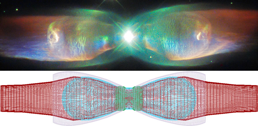
Fig. 1: PNe M2-9: Top image captured from NASA Hubble telescope and processed by Judy Schmidt, filters used: [S ii], [O iii] and H $\alpha$. Bottom image Shape 3D model. Top image reproduced from https://www.nasa.gov/feature/goddard/hubble-sees-the-wings-of-a-butterfly-the-twin-jet-nebula . Refer to Doyle et al. [2000] for more information regarding the morphology of M2-9.

High resolution imaging may detect shapes, however better understanding of the three dimensional structure is achieved when this data is coupled with spatially resolved, high resolution spectra to determine the kinematics of the gas within the nebula. To this end we present a new application and pipeline that uses Shape software to create 3D models with density, velocity and temperature properties. The output of this is a data-cube which is processed by PyCross to generate Cloudy photoionisation models of nebulae. This is achieved using an intuitive interactive graphical user interface (GUI) that does not require programming experience, execution scripts or the need to install additional compilers or libraries. The paper outline is as follows: Section 2 discusses the development, installation, functionality and operational overview of PyCross. Section 3 demonstrates PyCross’ scientific pipeline outlining its use on novae V5668 Sagittarii (2015) and V4362 Sagittarii (PTB 42). Section 4 again demonstrates the pipeline for PN LoTr1. Section 5 consists of our discussion and conclusions.

Fig. 2: PyCross Operational Flowchart. Steps for generating new models, updating archived models by modifying Cloudy parameters and visualising current and archived models. A high-level overview of the path to generate a new model is illustrated in Fig. 3.

2 PyCross

The steep learning curves encountered when installing, understanding and utilising specialist software are further compounded when astronomers are often required to develop/code software for specific tasks. Momcheva and Tollerud [2015] carried out a survey, between December 2014 and February 2015, that focused on the use of software and the software skills of participants in the astronomy community worldwide. Participants consisted of 1142 astronomers ranging from students to postdocs and research scientists. All survey participants responded “yes” when asked if they used software as part of their research; 11% of responders said they used software developed by others; 57% used software developed by themselves and others; while 33% said they used software they developed themselves for specific purposes, as there was no software readily available. This research also revealed the open source language, Python, to be the programming language of choice.

With advances in techniques, hardware and software it is of no surprise the number of astronomy software applications made available has increased considerably over the last decade. More recently Fitzgerald et al. [2019] developed a standalone application (written in Python) for plotting photometric Colour Magnitude Diagrams (CMDs) using object orientated programming (OOP), a formal Software Design Lifecycle (SDLC) and Test Driven Development (TDD). This stand alone application worked “out of the box” required no installation of any additional software to function and emphasised the importance of quality and standards when developing software for astronomy. A SDLC defines a structured sequence of stages in software engineering to develop the intended software product, a TDD approach relies on a shorter development cycle, where requirements become specific test cases that the software must pass and OOP allows developers to break software projects down into smaller, more manageable modular problems, one object at a time.

2.1 Software development

PyCross was developed and tested on OSX using the PyCharm IDE (integrated development environment) 2018 Community Edition, Python 2.7 with later iterations using Python 3.7. The free community edition of PyCharm offers usage of both testing frameworks and code analysis tools. There were 24 iterations of this application before the code was “Frozen”, for this release, allowing for the creation of a single executable file that can be distributed to users. A frozen application contains all the code and any additional resources required to run the application, and includes the Python interpreter that it was developed on. The major advantage for distributing applications in this manner is that it will work immediately, without the need for the user to have the required version of Python (or any additional necessary libraries) installed on their system. A disadvantage of generating a single file is that it will be large (approximately 183 MB), as all necessary libraries are incorporated, the increase in file size is acceptable when considering other issues, for example ease of installation, running, and portability to other platforms. The Agile SDLC and TDD approaches employed in Fitzgerald et al. [2019] were adapted in the development of this software, refer to this text for a comprehensive review of employing specific SDLC and TDD approaches in astronomy. The remainder of this section will outline installation, features and operational overview of the functionality when using PyCross

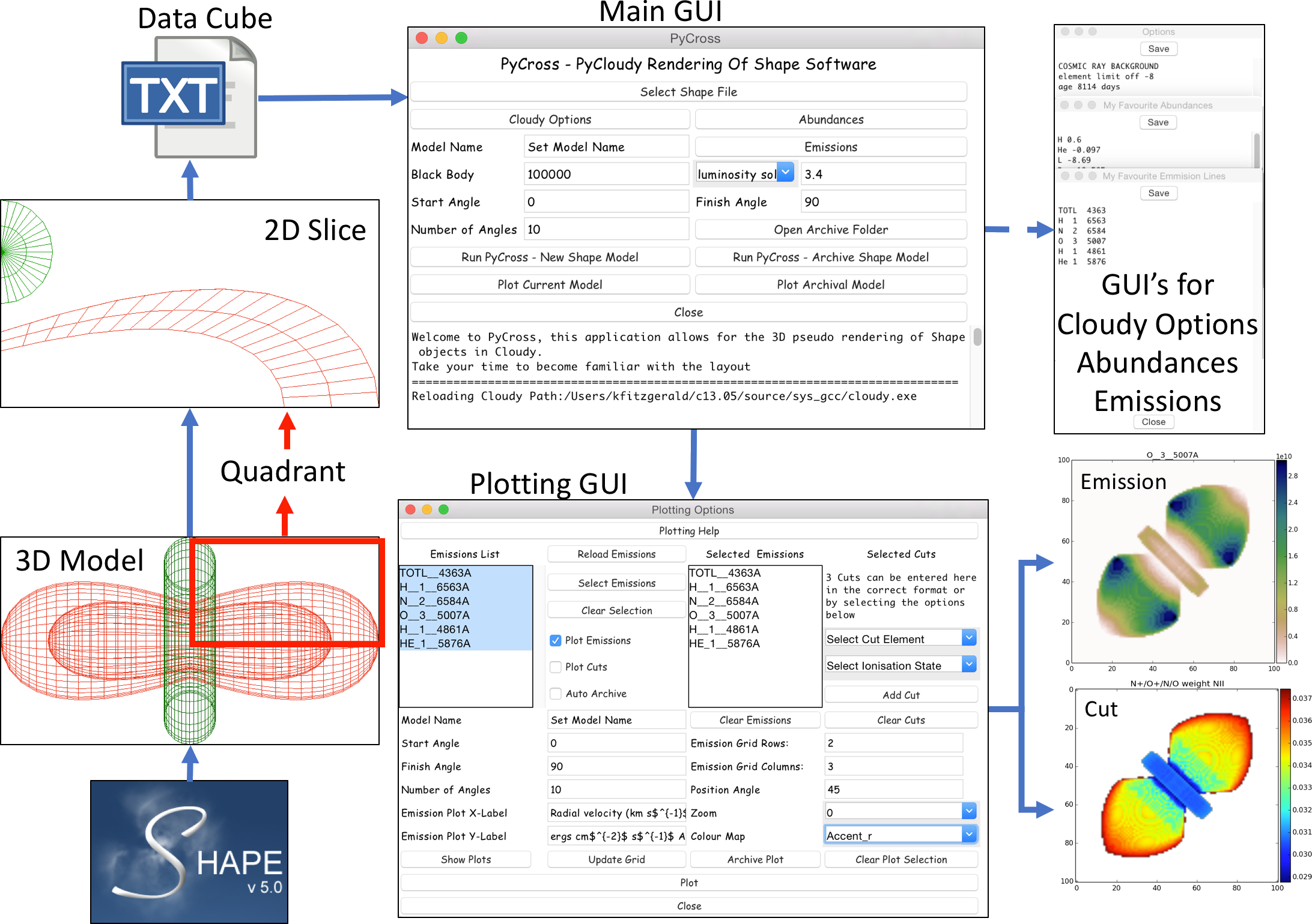
Fig. 3: A high level operational overview following the path for creating a new model outlined in Fig. 2. A new 3D Shape model is created with appropriate structure, densities and velocities. A quadrant of the overall model is then sliced to produce a data cube, in the format of a text file (subsection 2.3), which is inputted into PyCross. Cloudy options/parameters are then specified and the model is run. PyCross’s console will update informing the user of the progress. Once completed the user opens the plotting interface to plot the photoionisation and cut models (see bottom right of diagram) at different angles and inclinations. Colour map used for emission is gist_earth_r, one of 71 available to users. The model used here was designed as a theoretical nova with cosmic ray background and an approximate age of 8114 days, blackbody effective temperature of $50\times 10^{3}$ K, luminosity of $3.6\,\mathrm{L_{\odot}}$ and equatorial expansion velocity of $500\,\rm{km\,s^{-1}}$ and position angle of 45°. This model is available online at https://github.com/karolfitzgerald/PyCross_OSX_App, filename: Demo1.zip. A scientific approach for determining optimum Cloudy parameters is outlined in Fig. 8

2.2 PyCross functionality

PyCross was comprehensively designed to allow for intuitive usability while also providing automated features allowing the user to be more productive. A high-level operational overview of PyCross functionality is outlined in the operational flowchart in Fig. 2. Then, Fig. 3 follows the path for generating PyCross photoionisation rendering of a 3D Shape model utilising the application’s two main GUIs, for creating and plotting models. Smaller windows are used to manage any Cloudy preferences.

2.2.1 Installation & directory setup

As previously discussed, this application is “frozen” allowing for the creation of a single executable which contains all code and any additional python libraries to run. The only requirement is that Cloudy is pre-installed on the user’s system prior to running this programme.

A new directory structure is created in the root folder of the users computer when PyCross is loaded for the first time. This folder is named “PyCrossArchive” and is the root/destination for all work generated by the application: the following folders and files are generated upon startup and modified during the execution of a model:

• Model-Name-Timestamp.zip: PyCross models are automatically saved using the name assigned followed by a time-stamp of when they are created. The purpose of this is as follows: 1) To archive all models, this allows users the opportunity to review any change in parameters and resulting models generated. 2) A basic model can generate in excess of 100 files, each approximately 14.4 MB in size. While maintained within a well structured directory this can quickly consume disk space when generating a lot of models. Automatically zipping outputs to a single file significantly reduces file sizes (to approximately 3 MB zipped for a 14.4 MB un-zipped file) while also making it easier to process data at a later stage. For example, when handling these archived models, PyCross automatically extracts the contents of the selected zipped file into a temporary folder, and when finished the contents of the temporary folder are deleted. A time-stamp incorporated into the file name allows users to distinguish between models, if the model name does not change.

  • LogFile.txt: A text file that records the parameters used by the user and information relating to the progress of a model as it is being run. This information is also displayed on the main GUI. This file can be used at a later stage to compare models based on their parameters but also to recreate models if needed.

  • MakeData: This folder contains the output files generated by Cloudy based on the Shape model.

  • TempData: This folder contains data generated by PyCross that allows Cloudy to run the selected Shape model. It is also used to extract archive model data when modifying or plotting archived models.

• Plots: This folder contains the following sub-folders which store the generated plots of a model based on their type. Each time plots are generated the contents of this folder are deleted and replaced with new plots.

  • Cuts: This folder contains plots of the cuts generated. Cuts will be plotted based on their element and ionisation state. An additional N⁺/O⁺/N/O weight Nii cut, adapted from PyCloudy, is also plotted and saved here.

  • Emissions: Folder containing plots of the generated emission simulations.

  • PlotArchiveInformation.txt: This text file is updated automatically each time new plots are generated and contains information relating to the parameters entered by the user in the plotting options GUI, Plot GUI (see Fig. 3), this feature is useful for tracking differences in plots based on their parameters.

• PlotArchive: All data generated and stored in the Plots folder can be exported here and automatically saved as zip files. This reduces time recreating plots at a later stage while also keeping track of parameters changed and carried out on Plot GUI:

  • Auto Archive: If this option is selected in the Plotting Options GUI then all current & subsequent data generated will automatically be exported to the PlotArchive folder as a zip file. If the user does not change the model name then the naming convention is updated to include the time generated, this ensures that no work is overwritten or lost.

  • Archive Plot: There is an archive current data option that can be accessed by clicking this button in the Plotting Options GUI.

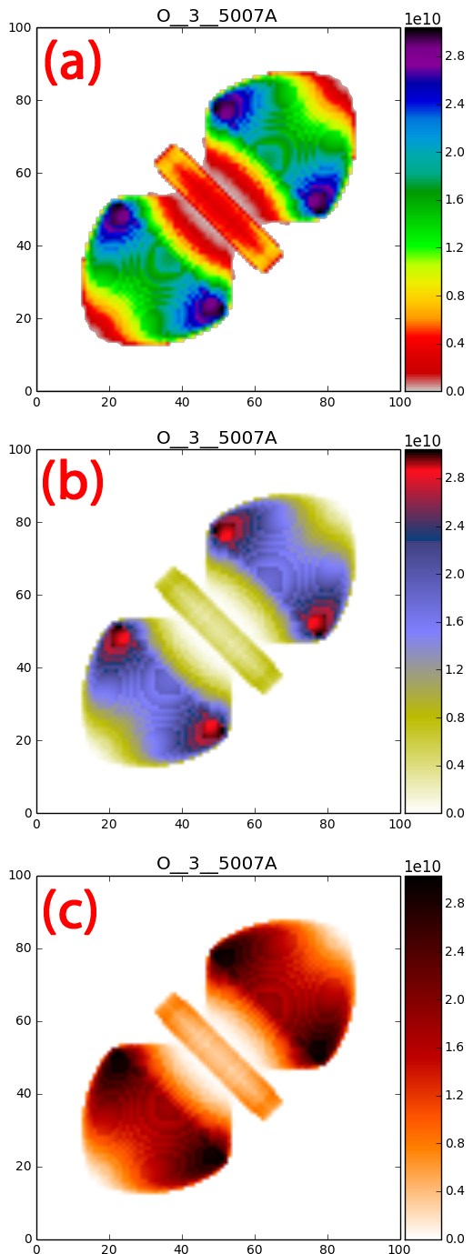
Fig. 4: Three colour map examples from a choice of 71. The emission model of [Oiii]  5007$\AA$ is derived from an example model (see Fig. 3) with a position angle of 45°. Colour-bars correspond to the effective temperature of the ionising source, flux units in ergs $\mathrm{s^{-1}}$. Scaled units of physical size are on x and y axes.

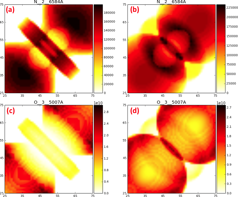
Fig. 5: Photoionisation models of [N ii]  6584$\AA$ (a, b) and [O iii]  5007$\AA$ (c, d) derived from the theoretical model in Fig. 3. Each emission plot initially plotted at an inclination angle of 90°(a, c) then at 50°(b, d). Colour-bars correspond to the effective temperature of the ionising source, flux units in ergs $\mathrm{s^{-1}}$. Plots are zoomed to better visualise features like the torus across different emissions and angles. The colour map used was hot_r.

2.3 Shape data cube text file

The Shape model is based on observational data and can be informed by a combination of narrow-band imaging, medium-high resolution spectroscopy and polarimetry. If these data types are not all at hand, then they can be used individually with the application of some theory or in certain combinations, given data of good quality. Integral field unit spectroscopy can be a particularly powerful observational tool to aid in the derivation of nebular morpho-kinematics. In this section the process on how to construct the output data cube from Shape for input into PyCross which is used in the MakeData and TempData files will be explained.

First users must derived the morphology of the nebular structure under study and assign a fixed or variable density structure. Next users must create a ‘cut’ of the nebula so it can be represented by a 2D array. To do this the user must place the nebula with its long axis pointing along the x-axis. Then a slice of a quarter of the major-axis of axisymmetric shape is taken, see Fig. 3 (2D Slice), Fig. 8, panel 2(a) and Fig. 9 (c). This is done in the Shape 3D module. Users must first go to the object primitive, then take a slice of the nebula by setting $\phi_{min}=90^{\degree}$, $\phi_{max}=180^{\degree}$, $\theta_{min}=-91^{\degree}$ and $\theta_{min}=-89^{\degree}$.

Once users have made an appropriate 2D slice of their nebula they move to the Shape render tab. In this tab the renderer must be set to be Physical. The slit and image geometries are set to be square such that they overlap and cover the entirety of the 2D slice, again refer to Fig. 3 (2D Slice), Fig. 8, panel 2(a) and Fig. 9 (c) for how the structure should appear in the image render window. Finally users set up a text file to output the position and velocities along the x, y and z axes (Px, Py, Pz, Vx, Vy Vz) along with the corresponding density and temperature. This is done under “Render” in the Parameters section of Shape. When users click the Render button a text file will be generated in a folder designated by the user. This text file is then imported directly into PyCross via its GUI. Currently only Px, Py, Pz and density arguments are used as input to the PyCross simulations. Temperature and velocity information will be utilised in the next iteration of PyCross.

2.3.1 User Interface & Operational Overview

The Graphical user interface (GUI) is designed to be as intuitive as possible and consists of two main GUI windows. The first allows the user to set parameters and run models while the second controls the plotting, these interfaces pass information to each other to enhance efficiency. Other GUIs allow users to set additional Cloudy options, emission lines and abundances. The operational flowchart of this application is illustrated in Fig. 2 and a high level overview of the GUIs taking the path of a new model is illustrated in Fig. 3. A scientific approach to determine optimum Cloudy parameters is discussed in section 3 (see Fig. 8). Once a Shape model, with a suitable morphology, density and velocity have been created it is then placed at an inclination of 90°. This 3D model must be represented two dimensionally, by taking a 2D slice of one quarter of the model. A data cube is created that describes the velocity and density at each position in the shell, this is processed by PyCross. A series of 1D Cloudy simulations are computed along the 2D Shape model slice. Lastly, the 2D photoionisation map is wrapped and flipped in order to create the full pseudo 3D photoionisation model. Currently this technique is constrained to axisymmetric nebulae, but as discussed later this allows for the modelling of a large majority of PNe and novae.

The main GUI allows users to set the name of the current model, blackbody temperature, total luminosity, angle range (start-finish) and the number of angles in the range. Cloudy preferences for the model general input, i.e. options, abundances and emissions are entered into smaller windows and when saved, will remain when the programme is started again. There is no limit to the number of parameters entered into these windows provided that they conform to valid Cloudy commands. This removes any learning curve, complex commands and the need to run shell scripts, thus increasing productivity. Once a model is successfully created the emissions list, set in the main GUI will be available and visible for selection in the plotting option GUI. Button functionality on the main GUI is as follows:

• Select Shape File: Allows the user to select the .txt data cube output from Shape (see subsection 2.3).

• Cloudy Options: Opens up a new window allowing the user to type/paste Cloudy options, visible at the top left of Fig. 3. For example when creating a model for a nova, options might include:
  
  “cosmic ray background
  element limit off -8
  age 8114 days”
  

• Abundances: Opens a new window allowing the user to type/paste abundances to be used as input to the model. Examples of abundances can be found by clicking Reference $|$ Abundance Examples in the menu bar.

• Emissions: Opens a new window allowing the user to type/paste emissions to be used as input to the model. Emissions must be added in a particular format of no more than 10 characters. To ensure that emissions are entered correctly, PyCross has an extensive library of emission lines that is available by clicking Reference $|$ Emission Line Index on the menu bar.

• Open Archive Folder: Opens a new Finder/Explorer window where all PyCross data is stored.

• Run PyCross - New Shape Model: This button is clicked to run a new model; the user must first have selected a Shape data cube and entered all necessary Cloudy options.

• Run PyCross - Archive Shape Model: If users create a model and are not satisfied with the outcome or feel that certain parameters need to be changed then they can modify specific Cloudy options outlined above. By clicking this button and selecting an archived model, users can run the model again with updated parameters. This feature saves a lot of time as it does not require the user to start anew.

• Plot Current Model: Open the plotting GUI to plot the current PyCross model. Any emissions entered will automatically be loaded into the plotting options window.

• Plot Archive Model: Select a zipped archived model then open the plotting GUI and proceed to plot. This again saves time not having to create a model from the start, while also offering the user the choice of building a database of models to plot from.

An $`$emission’ as discussed here is a simulated narrow-band image at the wavelength of a specific spectral emission line. Users can plot from one to a maximum of six emissions (plotted in flux units ergs $\mathrm{s^{-1}}$) in a single plot by highlighting desired emission, and adding them to the “Selected Emissions” list. Once selected, a plotting grid can be adapted to fit the required number of emissions. The number of angles, inclination and labels for x-axis and y-axis are set prior to plotting. Corresponding emission lines will also be displayed at the top of each plot regardless of the number of plots/subplots, the effective temperature of the ionising source is located in the colour-bar to the right of each model.

Users can view a plot $`$cut’ with a weighted by Nii of N⁺/O⁺/N/O, which is automatically generated. These weighted plots are adapted from the tutorial for PyCloudy [Morisset, 2013], where one of the foundations that PyCross was developed on and show the ionised fraction versus neutral fraction for the two most commonly studied astrophysical metals, i.e. O and N. Selection of the cuts is performed by first selecting an element, then its ionising state; a maximum of three cuts is allowed per plot. Users may open the plotting folder directly from this GUI and automatically archive all plots generated in that session. This is achieved by selecting the Auto Archive checkbox; archive plots are saved using the name and time-stamp of creation similar to saving of newly generated models discussed earlier.

The latest version of PyCross includes the functionality that gives users the ability to plot in 71 different colour maps and magnify the centre regions of nebulae, allowing to better visualise regions and/or possible hidden features, see Fig. 4 and Fig. 5. On analysis of Fig. 4, the outer regions of the lobes are more clearly defined in (a) than (b) or (c) where the following colour maps were applied: (a) nipy_spectral_r, (b) gist_stern_r and (c) gist_heat_r. Colour maps may be misleading, for example differences of regions within the outer lobes of (a) and (b) in Fig. 4 are greatly exaggerated as compared to that in (c) which is more realistic. Offering this feature allows users to find a trade off for investigating features of nebulae.

The axes on all plots are normalised distance units (0-100), the colour-bar corresponds to the effective temperature of the ionising source, flux units in ergs s-1. Users can add additional text to the axis labels via the Plotting Options GUI, see Fig. 3. Mathematical notation can also be written for the plot axis labels when using a subset TeX markup by placing text inside a pair of dollar signs ($).

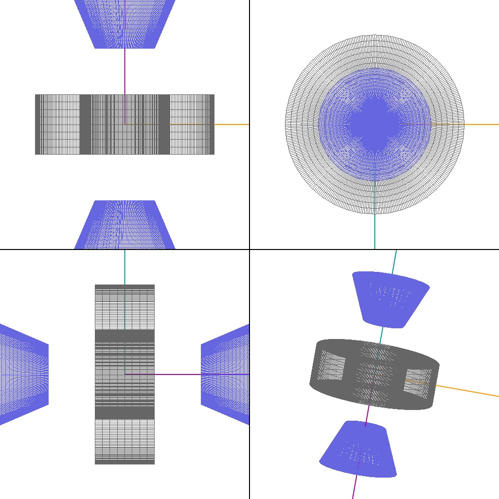
Fig. 6: Shape model for V5668 Sgr. Figure adapted from Harvey et al. [2018]

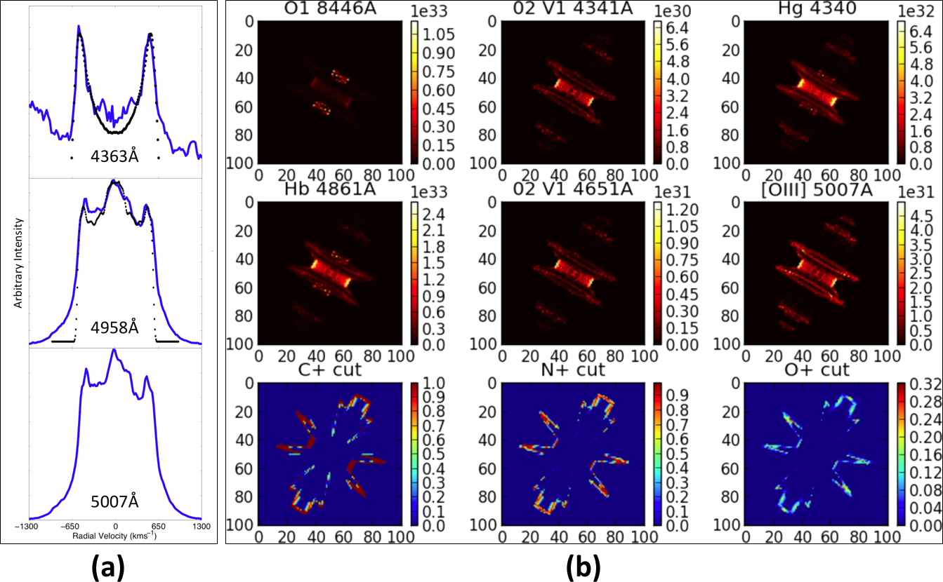
Fig. 7: (a) Spectral line profile simulations of [O iii] nebular and auroral lines of V5668 Sgr on day 822 post discovery. The blue-solid lines represent observed line profiles and were used in the fitting of a morpho-kinematical model with the Shape software, represented by overlaid black dots. The auroral line is fitted with an equatorial disk whereas the nebular lines fit an equatorial waist and polar cones morphology with a Hubble outflow velocity law. (b) PyCross emission models of V5668 Sgr, using nova abundances with the inclination angle set at 85°. Clumpiness was simulated using a Perlin noise modifier in Shape. The geometry used for this model is illustrated in Fig. 6. Figure adapted from Harvey et al. [2018], OII 4341$\AA$ was shown to demonstrate that the line emission is expected to arise from the same geometrical location and so to deblend it with 4340$\AA$ the same line profile shape would be assumed. With regard to the two nebular [O iii] lines they were shown in Harvey et al. [2018] to show the consistency in the line shape as would be expected from 4959$\AA$ and 5007$\AA$ [O iii] and how different the auroral [O iii] line shape was. Colour-bars correspond to the effective temperature of the ionising source, flux units in ergs $\mathrm{s^{-1}}$. PyCross scientific pipeline is illustrated in Fig. 8

3 PyCross pipeline applied to novae

Novae are the result of an eruption on the surface of a white dwarf in a close binary system. The white dwarf’s counterpart is normally a red dwarf or sub-giant, which has overfilled its Roche lobe and thus loses mass through an accretion stream onto the white dwarf surface. Pressure at the white dwarf-accreted envelope interface increases due to a buildup of hydrogen-rich material, eventually resulting in thermonuclear runaway. This subsequent eruption reaches luminosities $\gtrsim 10^{4}~{}\mathrm{{\rm L}_{\odot}}$, and ejects a mixture of material. A combination of that processed in the thermonuclear runaway, material dredged up from the white dwarf and the previously accreted outer layers of its companion. The ejected material reaches velocities of order $10^{3}$–$10^{5}\,\rm{km\,s^{-1}}$. Emission line profiles indicate considerable spatial density and velocity structure. Immediately after a nova eruption the ejected material is dense, bright and optically thick. This soon fades after revealing H i and He i emission lines. Over time [O iii], [N ii] and [Ne iii] become stronger relative to the fading continuum [Williams, 2012]. Over a few years the ejecta will be observed as a fading, constant-velocity expanding nebulous shell surrounding the post-nova star. These eruptions are not destructive enough to change either star and generally they return to their quiescent state, on decadal timescales. Classical novae repeat the process every $\sim\,10^{4}\,\mbox{--}10^{5}\,\rm{yr}$ [Osterbrock and Ferland, 2006]. Although, a recurrent nova population also exists, with observed recurrence periods on human timescales. Shorter rates of recurrence are related to heightened accretion rates onto higher mass white dwarfs [Prialnik and Kovetz, 1995, Yaron et al., 2005, Shara et al., 2010]. The material ejected from the white dwarf surface generally forms an axisymmetric shell of gas and dust around the system. These 3D shell structures are difficult to untangle as viewed on the plane of the sky without additional velocity information.

While spectroscopic data can be used to yield approximate values for temperature, velocity, and density along the line of sight of the object, a photoionisation model is required to determine the chemical structure of a nebula [Bohigas, 2008]. As discussed in Harvey et al. [2018], photoionisation modelling of ejected nova shells during their nebular stage of evolution can contribute to estimates of the total mass and abundances of heavy elements ejected during nova events [Helton et al., 2011]. Examples of the ability to realise photoionisation models of novae, more specifically V5668 Sgr and V4362 Sgr, created by the PyCross pipelines, are outlined in subsection 3.1 and subsection 3.2.

3.1 Nova: V5668 Sagittarii (2015)

Harvey et al. [2018] investigated V5668 Sgr (2015), a slow-evolving extremely bright nova on the surface of a CO white dwarf. The nova event produced dust [Gehrz et al., 2018], and was classified to be of the DQ Her-type. The V5668 Sgr nova event holds the record for longest sustained gamma ray emission from such an event [Siegert et al., 2018].

A goal of this research is to better understand the early evolution of classical nova shells in the context of the relationship between polarisation, photometry, and spectroscopy in the optical regime. Observations over five nights with the Dipol-2 instrument mounted on the William Herschel telescope (WHT) and the Royal Swedish Academy of Sciences (KVA) stellar telescope La Palma, yielded polarimetric data directly following the nova’s dust formation episode. While this nova shell is not yet resolvable with medium sized ground-based telescopes, Harvey et al. [2018] utilised PyCross to model and visualise the ionisation structure of V5568 Sgr. The polarimetric and spectroscopic data revealed conditions present in the expanding nova shell allowing for the creation of a Shape model. The proposed geometry consisted of an equatorial waist and polar cones, see Fig. 6.

Initial models consisted of broad parameter sweeps that were refined using PyCloudy [Morisset, 2013]. This allowed examination of emission line ratios for the hot–dense–thick nova shell under study. A cylindrical primitive was used to construct the equatorial waist, where a density, thickness and Hubble velocity law were applied. The polar features were constructed using cone primitives. In this instance densities applied were estimations from Cloudy simulations and velocity components were derived from measuring Doppler broadened characteristics of observed emission lines. Emission lines in fast outflows of unresolved structures are governed by their velocity field and orientation towards the observer. Analysis techniques available in Shape allow users to disentangle projection effects. The line shapes modelled in Fig. 7 (a) are displayed at an inclination of 85°, a polar velocity of $940\,\rm{km\,s^{-1}}$ and an equatorial velocity of $640\,\rm{km\,s^{-1}}$ at their maximum extensions.

Emission models of V5668 Sgr, were created using optimum values derived from Cloudy/PyCloudy parameter sweeps. The average density was found to be $\sim 1.0\times 10^{9}\,\rm{cm^{-3}}$, luminosity and effective temperature were set to log($\rm{{L_{\odot}}}$) = 4.36 and $1.8\times{10^{5}}\rm{K}$ respectively. To recreate the nova conditions on day 141 post discovery an inner and an outer radius were set to $3.2\times 10^{14}\,\rm{cm}$ and $6.4\times 10^{14}\,\rm{cm}$, respectively. Fig. 7 (b) illustrates the PyCross emission models for V5568 Sgr, where a comparison of the locality of emission through the shell of the same species is presented in each column of three panels. These models show the ionic cuts for C, N and O, respectively. An ionic cut is a slice of the ionised structure for a specific ionisation state of a species. Fig. 7 presents the first state of ionisation for C, N and O. The colour-bar shows the ionised fraction for different geometrical locations of the appropriate ionisation state.

Harvey et al. [2018] revealed variability in polarisation suggesting internal shocks in the nova outflow, supported by the presence of gamma-ray emission [Siegert et al., 2018]. The position angle of this nova was determined using the polarimetry observations. Spectroscopy allowed for derivation of the physical conditions, including outflow velocity and structure, nebular density, temperature and ionisation conditions. Photoionisation models generated from PyCross gave further insight into the nova system as a whole. Harvey et al. [2018] concluded that slow novae are regularly referred to “nitrogen flaring”, however based on their findings suggest that they are in fact more likely “oxygen flaring”.

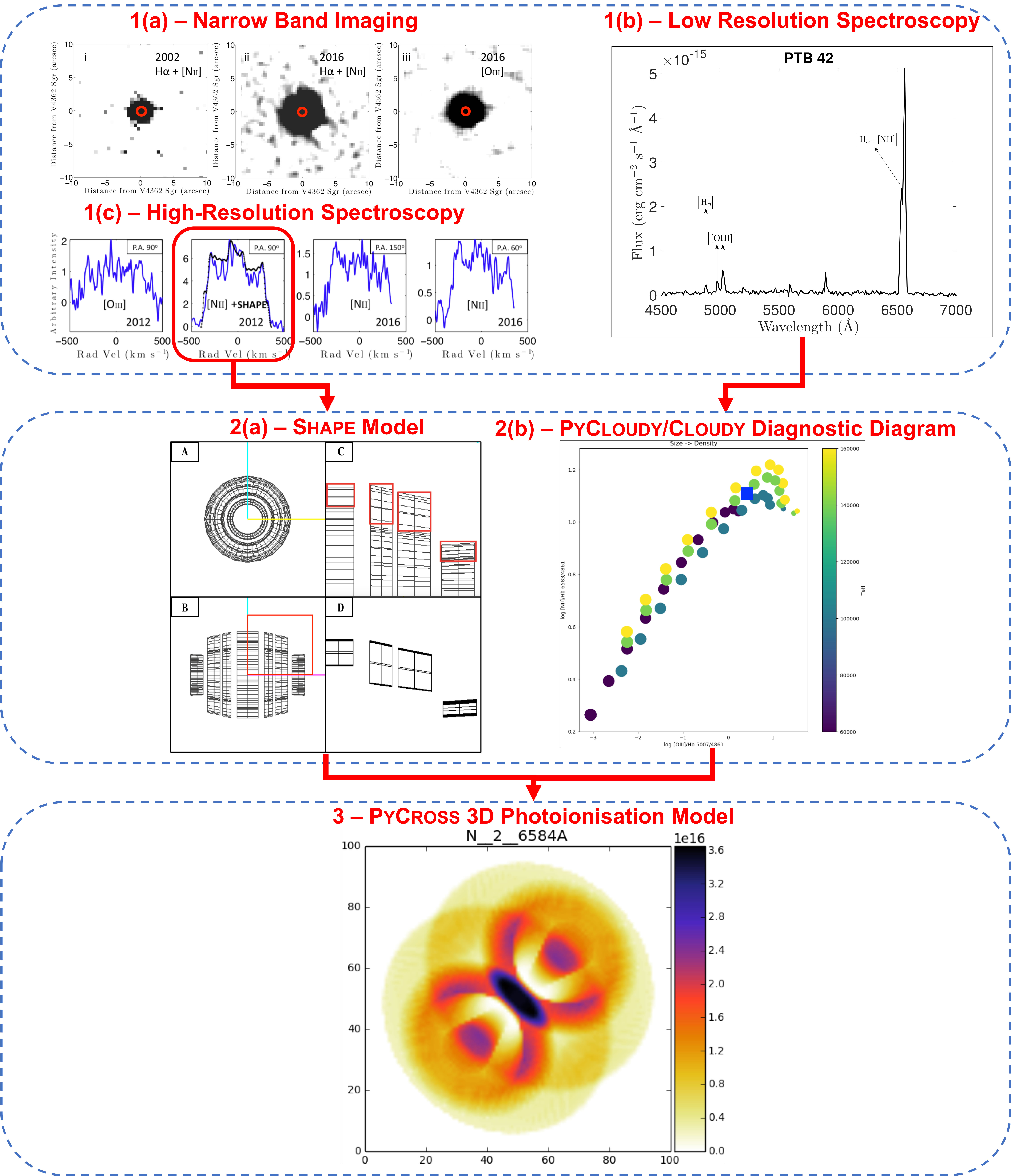
Fig. 8: PyCross Scientific Pipeline for V4362 Sgr / PTB 42(1994). This figure is split into three main sections (1-3). 1 represents observational data used to derive the spatial structure of an emission nebula, 1(a) is narrow-band imaging used to inform the extent and axial ratio of the nebula. 1(b) is low-resolution spectroscopy, used to derive density, abundances and ionisation conditions. 1(c) is high-resolution spectroscopy used to derive the velocity information for individual spectral lines. 2(a) is a suitable Shape geometry, seen in full in panels A and B, but arranged in panel D in a position to be output to a text file readable by PyCross, see section 2.3 and Harvey et al. [2020]. 2(b) is a diagnostic diagram generated to interpret the emission line ratios measured from broadband low-resolution spectra. 3 is the final output PyCross model generated from applying the geometry and density at each geometrical point (i.e. from the shape output text file). Other parameters such as the stellar luminosity, stellar effective temperature, and abundances are input to PyCross’s GUI. A set of 1D Cloudy simulations are run through the 2D parameter space which are then wrapped in azimuth around the complete shell creating a pseudo 3D model for any observable emission line, here we show the [Nii] 6584$\AA$ at a position angle of 60°. Colour-bars in 3 correspond to the effective temperature of the ionising source, flux units in ergs $\mathrm{s^{-1}}$, the colour-bar in the PyCloudy diagnostic diagram, 2(b), is the effective temp of the ionisation source. Figure adapted from [Harvey et al., 2020].

3.2 Nova: V4362 Sagittarii (PTB 42)

More recently [Harvey et al., 2020], utilised the current version of PyCross to aid in uncovering a previously undiscovered classical nova shell surrounding the nova system PTB 42 of the DQ Her type. Imaging was acquired from the Aristarchos telescope in Greece and consisted of two narrow-band filters; H $\alpha\,+\,[N\textsc{ii}]$ (6578$\AA/40\AA$) and [O iii] (5011$\AA/30\AA$) with exposures of 30 - 40 minutes in each filter. High-resolution spectroscopic data was obtained using the Manchester Echelle Spectrograph (MES) instrument mounted on the 2.1 m telescope at the San Pedro Mártir (SPM) observatory, Mexico. The PTB 42 nova shell, was detected using the low-resolution, high-throughput SPRAT spectrograph on the Liverpool Telescope during August of 2016. The PyCross pipeline (see Fig. 8) was then used to generate emission models based on imaging and spectroscopic observations. Based on these observations, the nova shell was reproduced in Shape and then passed to PyCross.

The P.A. for this target was chosen based on polarimetric observations presented in Evans et al. [2002], in addition to close examination of the major and minor axes in the narrow-band imaging (top left of Fig. 8). High-resolution spectroscopy from MES was used to find the radial velocity of individual components within the nova shell. Difficult to derive parameters are the system inclination, covering and filling factors of the nova shell, as well as the opening angle of the polar cones.

In this study a number of morpho-kinematic models were created to determine the best-fit relationship between image, PV array and 1D line spectrum to commonly proposed nova shells morphologies. While spatial information could not be resolved, structures within the nova could be resolved via line-of-sight velocities. The observed equatorial velocity is 350 km s^-1, as measured from the MES spectra. An axial ratio of 1.4 and polar velocity of 490 km s^-1 was initially chosen based on the inclination corrected axial ratio for similar novae DQ Her and T Aur [Bode and Evans, 2008]. Adjusting for inclination when fitting to the line profile gives an equatorial velocity of 390 km s^-1 and polar velocity of 550 km s^-1. This allowed for the remaining velocities to be set to 550$\,\times\,\rm{r/r0}$  (km s^-1). The observed [N ii] line profile, taken from the 2012 observation (seen encircled in red at the top left of Fig. 8, was chosen for modelling the nova shell structure as it had the highest S/N.

The luminosity of the system was estimated based on that of the class archetype, namely DQ Her, during quiescence Ferland et al. [1984]. The inner and outer radii of the shell are estimated based on the observed expansion velocity distribution and narrow-band imaging and shell age, although the actual shell thickness is difficult to know without resolving it spatially. Abundances used were for that of the archetypical slow nova, DQ Her [Ferland et al., 1984].

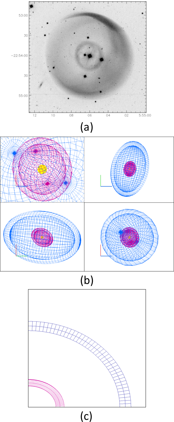
Fig. 9: (a) Deep, narrowband images of PN LoTr 1, in [O iii] 5007$\AA$. North is to the top of the image, East is to the left. Image acquired using European Southern Observatory (ESO) Multi-Mode Instrument (EMMI), mounted on the 3.6m New Technology Telescope (NTT) of La Silla Observatory. The outer shell appears brighter in both the northeast and southeast directions of the image, which could suggest the possibility of an inclined, elongated structure due to the projection effect. Image credit and ©  Tyndall et al. [2013]. (b) 3D Shape model of LoTr1 from different views. The view in the bottom right quadrant of (b) represents the nebula as in (a). (c) Shape quadrant slit of LoTr 1 where shells have being aligned. The resulting data cube is then passed to PyCross.

In this work PyCross was employed to better understand observed ionised nebula structure by using broadband spectra from which line ratios are measured. A grid of models was generated to determine the best fitting model parameters which were then applied through the derived geometry. This geometry is determined from matching line profiles in high-resolution spectra and narrow-band imaging in Shape. Polarimetry and imaging was used to determine the position angle of the shell. Using abundances adapted from the DQ Her nova shell model of Ferland et al. [1984] PyCross generated a pseudo 3D simulation of the ionisation structure of PTB 42 as seen in top centre of Fig. 8. Results show the difference in emission regions for the strongest nebular lines, i.e. [N ii] and [O iii]. The PyCross model presented in [Harvey et al., 2020] detailed observed components i.e. equatorial ring, higher latitude rings and polar features of the nova, allowing their individual behaviour to be examined.

4 PyCross pipeline applied to PNe

Post-main sequence low to intermediate mass stars ($\sim 0.8\,$M${}_{\odot}-8\,$M_⊙) will over time evolve to become planetary nebulae as the outer layers of the star are ejected through thermal pulses after the AGB phase. This exposes hotter layers that can ionise the previous ejected material. A detailed description of the evolutionary track and mechanics a star undergoes on its journey to become a PN at each phase is presented in Prialnik [2009] and see also [Herwig, 2005].

There are complications to this simple picture, particularly in the role of binarity and the possibility of ‘mimics’ such as symbiotic systems [Boffin and Jones, 2019]. As a result, there is no universal observational definition for PNe, but their existence is usually dependent on two components: a circumstellar shell of sufficient mass and density to be detectable, and a hot central star to ionise it. PNe candidates are usually discovered by objective-prism surveys or by direct imaging in a narrow spectral region around a strong emission line or line such as [O iii] 4959$\AA$, 5007$\AA$ or H $\alpha$ and [N ii] 6548$\AA$, 6583$\AA$ [Osterbrock and Ferland, 2006]. Their expanding shell sizes ($\sim$ 0.2 pc) and expansion velocities ($\sim$ 25 km s^-1) imply a dynamical lifetime of $\sim$ 10⁴ yr [Kwok, 2000].

As intermediate mass stars make up a large portion of the stellar mass in our galaxy, studying how their nuclear-processed interiors are ejected into intricate nebulae and eventually into the interstellar medium, can lead to a deeper understanding of the galaxy’s chemical evolution. PNe spectra are rich in emission lines, including the interesting forbidden lines, and serve as a laboratory for the physics and chemistry of photoionisation. Modelling the 3D spatiokinematic structure, along with the 3D photoionisation of PNe and their mimics can contribute to understanding how these spectacular nebulae are formed.

4.1 PN LoTr 1

The previous section described PyCross and its use in modelling and investigating novae emissions. In this subsection, and for the first time, PyCross will be used in modelling emissions for LoTr 1, a PN believed to contain a binary central star system consisting of a KL-type III giant and white dwarf, first discovered by Longmore and Tritton [1980].

A morpho-kinematic Shape model (Fig. 9 (a)) was created based on long-slit Echelle spectroscopy acquired using the Anglo-Australian Telescope/University College London Echelle Spectrograph (AATUCLES) and the New Technology Telescope-ESO Multi-Mode Instrument (NTT-EMMI) focused on the [O iii] 5007$\AA$ emissions over eight different slit positions, published in Tyndall et al. [2013]. Careful measuring of axes and relative sizes yielded a model constructed of two elongated shells with inner and outer shell radii of 5^′′ and 12^′′ respectively. Each shell is at different inclinations, with an angle of 50$\degree$ difference in position angle, and a difference of 57$\degree$ inclination (see Fig. 9 (a)). Modifiers were applied to elongate the inner and outer shells along the z-axis by a factor of 1.3 and 1.5 respectively.

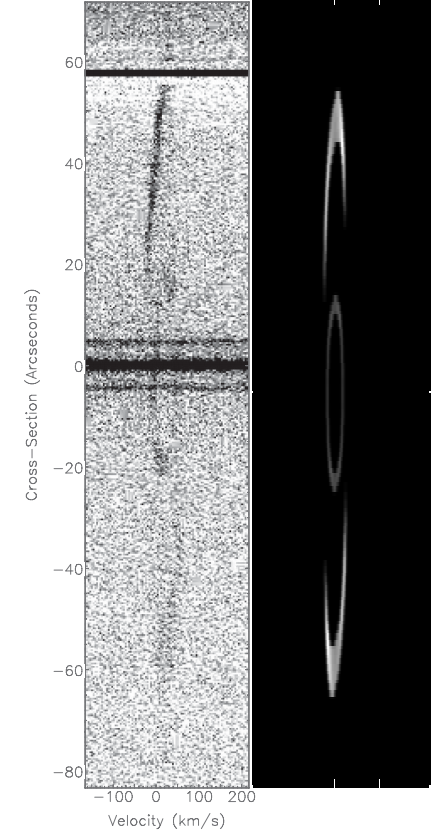
Fig. 10: Left: Recreation of slit position 1 acquired by Tyndall et al. [2013]. Right: Theoretical PV diagram created in Shape. West is up.

	Radius (cm)	Expansion Velocity (km/s)	Morphology	Kinematical Age (yrs)
Outer Shell	$2.84\times 10^{16}$	25 $\pm$ 4	Elliptical	35,000 $\pm$7,000
Inner Shell	$9.14\times 10^{15}$	17 $\pm$ 4	Elliptical	17,000 $\pm$ 5,500

Table 1: Table of parameters for both inner and outer shells of LoTr 1 from Tyndall et al. [2013].

A comparison of the first slit acquired by Tyndall et al. [2013] compared to that recreated in Shape can be seen in Fig. 10. The observed slit position is in the left hand panel and the right panel shows the theoretical PV array. The systemic velocity, V_sys of the central shell was determined to be 14 $\pm$ 4 km/s [Tyndall et al., 2013], for the observations, which result from the velocity axis of this data being relative to the V_sys. An important similarity correspond to the major axis in that it has the same length as the diameter of the inner shell. This contributes to the assumption that it is a closed, isolated structure rather than a bipolar nebula. A bipolar nebular structure viewed from above would not give this regular shape. These ellipses seen along the velocity axis appear symmetric in both images, in agreement with a spherical shell or elongated ovoids.

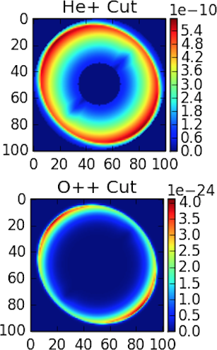
Fig. 11: LoTr 1 PyCross photoionisation cuts of He⁺ and O⁺⁺, using PN abundances with the inclination angle set at 40$\degree$. Colour-bars correspond to the effective temperature of the ionising source, flux units in ergs $\mathrm{s^{-1}}$.

Minor modifications were made to align the shells of LoTr1 prior to creating a data cube slice in order to create a photoionisation model using PyCross (Fig. 9 (b)). Default PN abudances were used from Aller and Czyzak [1983] and Khromov [1989], with high depletions for elements not listed. Emission models generated from PyCross for LoTr 1 can be seen in Fig. 12. These models are set at an inclination angle of 40$\degree$, with a blackbody effective temperature of $\sim$100,000 K [Gruendl et al., 2001] and a luminosity of 100 L_⊙ [Henry et al., 1999]. These parameters were chosen as they were ascertained from the Helix nebula (NGC 7293), one of the closest and brightest PN [Hora et al., 2006]. While a hot black body spectrum is used for the modelling here, it is possible to use more complex central star spectra such as, for example, WR-type spectra, as applicable to HB4 [Derlopa et al., 2019] and generally found in around 10% of PNe [DePew et al., 2011]. Fig. 11 shows ionic cuts of He⁺ and O⁺⁺, top and bottom respectively, at an inclination angle of 90$\degree$ for the left column, and 40$\degree$ for the right column. It is worth noting that the object appears entirely spherical at 90$\degree$ because this angle shows a cut through the object head on. Similar observations were made by Tyndall et al. [2013] who reported clear asymmetry in the nebular structure, additionally but it is close to a head on view.

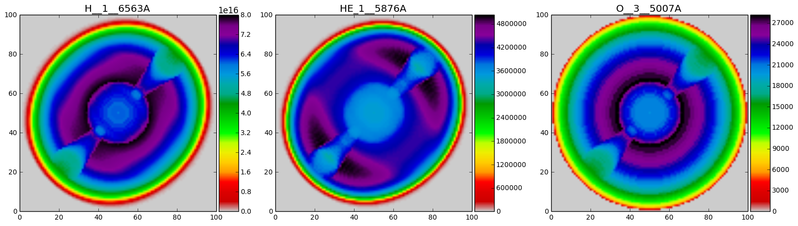
Fig. 12: LoTr 1 PyCross photoionisation model using PN abundances with the inclination angle set at 40$\degree$. The input Shape model is seen in Fig. 9 with changes made to the inclination angles of the two shells to make the entire object symmetrical. Colour-bars correspond to the effective temperature of the ionising source, flux units in ergs $\mathrm{s^{-1}}$.

In this scenario and for simplicity, attention is limited to two elements: oxygen and helium. While diffuse nebulae contain vast quantities of material, they have relatively low densities (approximately $10^{3}$ particles $\mathrm{cm^{-3}}$). They are rich with emission lines such as Balmer lines of hydrogen, as well as those which arise from the transitions between energy levels which result in ions such as O⁺, O⁺⁺, N⁺, etc. As the lifetime of ionised hydrogen is very short (fractions of a microsecond due to the fast nature of electric dipole transitions), the probability of excited hydrogen is negligible, so any hydrogen can be assumed to be in its ground state for the purpose of ionisation rate calculations.

Fig. 11 compares O⁺⁺ and He⁺ in our model for LoTr 1 showing predicted emissions maps of this PN in spectral lines other than those observed, to be compared with future observations. The stellar spectrum and nebular analysis could be developed further from this starting point based on more information regarding the central star. This would require a more extensive data-set for further investigation into the morphology of LoTr 1 in order to confirm its true structure and inclination. A data-set with a higher signal-to-noise ratio would be necessary to resolve the very faint outer shell.

Oxygen is a particularly useful ion in analysing the physical structure of a nebula. The well known [Oiii] 5007$\AA$ optical line strongly contributes to nebula cooling, while more highly ionised OVI lines can radiate in at higher energies in hotter parts of the nebula. Where ionised hydrogen is found, we expect to find ionised oxygen as the first ionisation potential of oxygen is almost identical to that of hydrogen. The difference between the two however, is that oxygen can be ionised more than once [Dyson and Williams, 1997].

5 Conclusion

A new application has been presented for the generation of photoionisation pseudo 3D modelling of thin shell nebulae modelled in Shape. Functionality, an operational overview and a scientific pipeline has been described with scenarios where PyCross has been adopted for novae and PN. The software was developed using a formal software development lifecycle, written in Python and will work without the need to install any development environments or additional python packages. This application, Shape models and PyCross archive examples are freely available to students, academics and research community on GitHub (https://github.com/karolfitzgerald/PyCross_OSX_App) for download. The authors cordially request that this paper be referenced when using this tool.

References

References

- Akras et al. [2016] Akras, S., Clyne, N., Boumis, P., Monteiro, H., Gonçalves, D.R., Redman, M.P., Williams, S., 2016. Deciphering the bipolar planetary nebula Abell 14 with 3D ionization and morphological studies. Monthly Notices of the Royal Astronomical Society 457, 3409–3419. doi:10.1093/mnras/stw038, arXiv:1601.02170.
- Aller and Czyzak [1983] Aller, L., Czyzak, S., 1983. Chemical compositions of planetary nebulae. The Astrophysical Journal Supplement Series 51, 211--247.
- Bode and Evans [2008] Bode, M.F., Evans, A., 2008. Classical Novae. Second ed., University Press.
- Boffin and Jones [2019] Boffin, H., Jones, D., 2019. The Importance of Binaries in the Formation and Evolution of Planetary Nebulae. SpringerBriefs in Astronomy, Springer International Publishing. URL: https://books.google.ie/books?id=9mGtDwAAQBAJ.
- Bohigas [2008] Bohigas, J., 2008. Photoionization models applied to planetary nebulae. The Astrophysical Journal 674, 954.
- Boyle [2018] Boyle, L., 2018. Planet engulfment and the planetary nebula morphology mystery. Ph.D. thesis. Centre for Astronomy, School of Physics, National University of Ireland, Galway.
- Boyle and Redman [2017] Boyle, L.A., Redman, M.P., 2017. Planet destruction and the shaping of planetary nebulae, in: Liu, X., Stanghellini, L., Karakas, A. (Eds.), Planetary Nebulae: Multi-Wavelength Probes of Stellar and Galactic Evolution, pp. 193--196. doi:10.1017/S1743921317000539.
- Clyne et al. [2014] Clyne, N., Redman, M.P., Lloyd, M., Matsuura, M., Singh, N., Meaburn, J., 2014. VLT observations of the asymmetric Etched Hourglass Nebula, MyCn 18. aap 569, A50. doi:10.1051/0004-6361/201322118, arXiv:1408.4030.
- Corradi et al. [2015] Corradi, R.L.M., García-Rojas, J., Jones, D., Rodríguez-Gil, P., 2015. Binarity and the Abundance Discrepancy Problem in Planetary Nebulae. The Astrophysical Journal 803, 99. doi:10.1088/0004-637X/803/2/99, arXiv:1502.05182.
- DePew et al. [2011] DePew, K., Parker, Q.A., Miszalski, B., De Marco, O., Frew, D.J., Acker, A., Kovacevic, A.V., Sharp, R.G., 2011. Newly discovered Wolf-Rayet and weak emission-line central stars of planetary nebulae. Monthly Notices of the Royal Astronomical Society 414, 2812--2827. doi:10.1111/j.1365-2966.2011.18337.x, arXiv:1101.2468.
- Derlopa et al. [2019] Derlopa, S., Akras, S., Boumis, P., Steffen, W., 2019. High-velocity string of knots in the outburst of the planetary nebula Hb4. mnras 484, 3746--3754. doi:10.1093/mnras/stz193, arXiv:1901.05767.
- Doyle et al. [2000] Doyle, S., Balick, B., Corradi, R.L.M., Schwarz, H.E., 2000. The evolving morphology of the bipolar nebula m2-9. The Astronomical Journal 119, 1339--1344. URL: https://doi.org/10.1086%2F301267, doi:10.1086/301267.
- Dyson and Williams [1997] Dyson, J.E., Williams, D.A., 1997. The physics of the interstellar medium. CRC Press.
- Ercolano [2005] Ercolano, B., 2005. New Advances in Photoionisation Codes: How and what for?, in: Szczerba, R., Stasińska, G., Gorny, S.K. (Eds.), Planetary Nebulae as Astronomical Tools, pp. 35--43. doi:10.1063/1.2146222, arXiv:astro-ph/0508683.
- Ercolano et al. [2003] Ercolano, B., Barlow, M.J., Storey, P.J., Liu, X.W., 2003. MOCASSIN: a fully three-dimensional Monte Carlo photoionization code. mnras 340, 1136--1152. doi:10.1046/j.1365-8711.2003.06371.x, arXiv:astro-ph/0209378.
- Evans et al. [2002] Evans, A., Yudin, R.V., Naylor, T., Ringwald, F.A., Koch Miramond, L., 2002. Broadband polarimetry of novae in outburst. Astronomy & Astrophysics 384, 504--512.
- Fang et al. [2018] Fang, X., Zhang, Y., Kwok, S., Hsia, C.H., Chau, W., Ramos-Larios, G., Guerrero, M.A., 2018. Extended Structures of Planetary Nebulae Detected in H2 Emission. apj 859, 92. doi:10.3847/1538-4357/aac01e, arXiv:1804.08840.
- Ferland et al. [1998] Ferland, G.J., Korista, K.T., Verner, D.A., Ferguson, J.W., Kingdon, J.B., Verner, E.M., 1998. CLOUDY 90: Numerical Simulation of Plasmas and Their Spectra. pasp 110, 761--778. doi:10.1086/316190.
- Ferland et al. [2013] Ferland, G.J., Porter, R.L., van Hoof, P.A.M., Williams, R.J.R., Abel, N.P., Lykins, M.L., Shaw, G., Henney, W.J., Stancil, P.C., 2013. The 2013 Release of Cloudy. Revista Mexicana de Astronomia y Astrofisica 49, 137--163. arXiv:1302.4485.
- Ferland et al. [1984] Ferland, G.J., Williams, R.E., Lambert, D.L., Shields, G.A., Slovak, M., Gondhalekar, P.M., Truran, J.W., 1984. IUE observations of DQ Herculis and its nebula, and the nature of the cold nova shells. apj 281, 194--204. doi:10.1086/162088.
- Fitzgerald et al. [2019] Fitzgerald, K., Browne, L.M., Butler, R., 2019. Using the agile software development lifecycle to develop a standalone application for generating colour magnitude diagrams. Astronomy and Computing 28, 100283. URL: http://www.sciencedirect.com/science/article/pii/S2213133718300556, doi:https://doi.org/10.1016/j.ascom.2019.05.001.
- Gehrz et al. [2018] Gehrz, R.D., Evans, A., Woodward, C.E., Helton, L.A., Banerjee, D.P.K., Srivastava, M.K., Ashok, N.M., Joshi, V., Eyres, S.P.S., Krautter, J., Kuin, N.P.M., Page, K.L., Osborne, J.P., Schwarz, G.J., Shenoy, D.P., Shore, S.N., Starrfield, S.G., Wagner, R.M., 2018. The Temporal Development of Dust Formation and Destruction in Nova Sagittarii 2015#2 (V5668 SGR): A Panchromatic Study. The Astrophysical Journal 858, 78. doi:10.3847/1538-4357/aaba81, arXiv:1804.00575.
- Gruendl et al. [2001] Gruendl, R.A., Chu, Y.H., O’Dwyer, I.J., Guerrero, M.A., 2001. Variable h line emission from the central star of the helix nebula. The Astronomical Journal 122, 308.
- Harvey et al. [2016] Harvey, E., Redman, M.P., Boumis, P., Akras, S., 2016. Modelling the structure and kinematics of the Firework nebula: The nature of the GK Persei nova shell and its jet-like feature. Astronomy & Astrophysics 595, A64. doi:10.1051/0004-6361/201628132, arXiv:1609.01363.
- Harvey et al. [2020] Harvey, E.J., Redman, M.P., Boumis, P., Akras, S., Fitzgerald, K., Dulaimi, S., Williams, S.C., Darnley, M.J., Lam, M.C., Kopsacheilli, M., Derlopa, S., 2020. Two New Nova Shells associated with V4362 Sagittarii and DO Aquilae. Monthly Notices of the Royal Astronomical Society Paper submitted.
- Harvey et al. [2018] Harvey, E.J., Redman, M.P., Darnley, M.J., Williams, S.C., Berdyugin, A., Piirola, V.E., Fitzgerald, K.P., O’Connor, E.G.P., 2018. Polarimetry and spectroscopy of the ‘‘oxygen flaring’’ DQ Herculis-like nova: V5668 Sagittarii (2015). Astronomy & Astrophysics 611, A3. doi:10.1051/0004-6361/201731741, arXiv:1802.00224.
- Helton et al. [2011] Helton, L.A., Evans, A., Woodward, C.E., Gehrz, R.D., 2011. Atypical dust species in the ejecta of classical novae, in: Joblin, C., Tielens, A.G.G.M. (Eds.), EAS Publications Series, pp. 407--412. doi:10.1051/eas/1146042.
- Henry et al. [1999] Henry, R., Kwitter, K., Dufour, R., 1999. Morphology and composition of the helix nebula. The Astrophysical Journal 517, 782.
- Herwig [2005] Herwig, F., 2005. Evolution of Asymptotic Giant Branch Stars. Annu. Rev. Astron. Astrophys 43, 435--479. doi:10.1146/annurev.astro.43.072103.150600.
- Hora et al. [2006] Hora, J.L., Latter, W.B., Smith, H.A., Marengo, M., 2006. Infrared observations of the helix planetary nebula. The Astrophysical Journal 652, 426.
- Khromov [1989] Khromov, G., 1989. Planetary nebulae. Space Science Reviews 51, 339--423.
- Kwok [2000] Kwok, S., 2000. The Origin and Evolution of Planetary Nebulae. Cambridge Astrophysics, Cambridge University Press. doi:10.1017/CBO9780511529504.
- Longmore and Tritton [1980] Longmore, A., Tritton, S., 1980. A second list of new planetary nebulae found on united kingdom 1.2-m schmidt telescope plates. Monthly Notices of the Royal Astronomical Society 193, 521--524.
- Luridiana, V. et al. [2015] Luridiana, V., Morisset, C., Shaw, R. A., 2015. Pyneb: a new tool for analyzing emission lines - i. code description and validation of results. Astronomy & Astrophysics 573, A42. URL: https://doi.org/10.1051/0004-6361/201323152, doi:10.1051/0004-6361/201323152.
- McLaughlin [1942] McLaughlin, D.B., 1942. Spectral Stages of Novae. apj 95, 428. doi:10.1086/144414.
- Momcheva and Tollerud [2015] Momcheva, I., Tollerud, E., 2015. Software Use in Astronomy: an Informal Survey. ArXiv e-prints arXiv:1507.03989.
- Morisset [2013] Morisset, C., 2013. pyCloudy: Tools to manage astronomical Cloudy photoionization code. Astrophysics Source Code Library. arXiv:1304.020.
- Osterbrock and Ferland [2006] Osterbrock, D.E., Ferland, G.J., 2006. Astrophysics of gaseous nebulae and active galactic nuclei. 2nd ed.
- Peimbert et al. [2017] Peimbert, M., Peimbert, A., Delgado-Inglada, G., 2017. Nebular Spectroscopy: A Guide on Hii Regions and Planetary Nebulae. Publ. Astron. Soc. Pac 129, 082001. doi:10.1088/1538-3873/aa72c3, arXiv:1705.06323.
- Prialnik [2009] Prialnik, D., 2009. An Introduction to the Theory of Stellar Structure and Evolution. Cambridge University Press.
- Prialnik and Kovetz [1995] Prialnik, D., Kovetz, A., 1995. An Extended Grid of Multicycle Nova Evolution Models. The Astrophysical Journal 445, 789. doi:10.1086/175741.
- Sabin et al. [2017] Sabin, L., Gómez-Muñoz, M.A., Guerrero, M.A., Zavala, S., Ramos-Larios, G., Vázquez, R., Corral, L., Blanco Cárdenas, M.W., Guillén, P.F., Olguín, L., Morisset, C., Navarro, S., 2017. Catching a grown-up starfish planetary nebula - I. Morpho-kinematical study of PC 22. mnras 467, 3056--3065. doi:10.1093/mnras/stx295, arXiv:1702.00029.
- Santander-Garcia et al. [2017] Santander-Garcia, M., Bujarrabal, V., Alcolea, J., Castro-Carrizo, A., Sánchez Contreras, C., Quintana-Lacaci, G., Corradi, R.L.M., Neri, R., 2017. ALMA high spatial resolution observations of the dense molecular region of NGC 6302. aap 597, A27. doi:10.1051/0004-6361/201629288, arXiv:1609.06455.
- Shara et al. [2010] Shara, M.M., Yaron, O., Prialnik, D., Kovetz, A., Zurek, D., 2010. An Extended Grid of Nova Models. III. Very Luminous, Red Novae. The Astrophysical Journal 725, 831--841. doi:10.1088/0004-637X/725/1/831, arXiv:1009.3864.
- Siegert et al. [2018] Siegert, T., Coc, A., Delgado, L., Diehl, R., Greiner, J., Hernanz, M., Jean, P., José, J., Molaro, P., Pleintinger, M.M.M., Savchenko, V., Starrfield, S., Tatischeff, V., Weinberger, C., 2018. Gamma-ray observations of Nova Sgr 2015 No. 2 with INTEGRAL. Astronomy & Astrophysics 615, A107. doi:10.1051/0004-6361/201732514, arXiv:1803.06888.
- Steffen et al. [2011] Steffen, W., Koning, N., Wenger, S., Morisset, C., Magnor, M., 2011. Shape: A 3D Modeling Tool for Astrophysics. IEEE Transactions on Visualization and Computer Graphics, Volume 17, Issue 4, p.454-465 17, 454--465. doi:10.1109/TVCG.2010.62, arXiv:1003.2012.
- Torres-Peimbert [2015] Torres-Peimbert, S., 2015. Chemical composition of planetary nebulae: The abundance discrepancy problem, in: American Institute of Physics Conference Series, p. 040003. doi:10.1063/1.4937639.
- Tyndall et al. [2013] Tyndall, A., Jones, D., Boffin, H., Miszalski, B., Faedi, F., Lloyd, M., Boumis, P., López, J., Martell, S., Pollacco, D., et al., 2013. Two rings but no fellowship: Lotr 1 and its relation to planetary nebulae possessing barium central stars. Monthly Notices of the Royal Astronomical Society 436, 2082--2095.
- van Hoof et al. [2000] van Hoof, P.A.M., Martin, P.G., Ferland, G.J., 2000. Current Development of Cloudy, in: Franco, J., Terlevich, L., López-Cruz, O., Aretxaga, I. (Eds.), Cosmic Evolution and Galaxy Formation: Structure, Interactions, and Feedback, p. 220. arXiv:astro-ph/0001196.
- Williams [2012] Williams, R., 2012. Origin of the ‘‘He/N’’ and ‘‘Fe II’’ Spectral Classes of Novae. The Astronomical Journal 144, 98. doi:10.1088/0004-6256/144/4/98, arXiv:1208.0380.
- Yaron et al. [2005] Yaron, O., Prialnik, D., Shara, M.M., Kovetz, A., 2005. An Extended Grid of Nova Models. II. The Parameter Space of Nova Outbursts. The Astrophysical Journal 623, 398--410. doi:10.1086/428435, arXiv:astro-ph/0503143.