Magnetic field induced topological nodal-lines in triplet excitations of frustrated antiferromagnet CaV₄O₉

Abstract

Magnetic field induced multiple non-Dirac nodal-lines are found to emerge in the triplet dispersion bands of a frustrated spin-1/2 antiferromagnetic model on the CaVO lattice. Plaquette and bond operator formalisms have been employed to obtain the triplet plaquette and bond excitations for two different parameter regimes in the presence of nearest and next-nearest-neighbor Heisenberg interactions based on the plaquette-resonating-valence-bond and dimerized ground states, respectively. In the absence of magnetic field a pair of six-fold degenerate nodal-loops with distinct topological feature is noted in the plaquette excitations. They are found to split into three pairs of two-fold degenerate nodal-loops in the presence of magnetic field. In the other parameter regime, system hosts two-fold degenerate multiple nodal-lines with a variety of shapes in the triplon dispersion bands in the presence of magnetic field. Ground state energy and spin gap have been determined additionally for the two regimes. Those nodal-lines are expected to be observed in the inelastic neutron scattering experiment on the frustrated antiferromagnet, CaV₄O₉.

I INTRODUCTION

Studies on topological states of matter are continuing with great interest in the recent times for the understanding of their various symmetry protected properties. Topological matter is broadly classified as topological insulator (TI) and topological semimetal (TSM) besides the topological superconductor. In contrast to TI, TSM has semimetallic bulk state in addition to metallic surface states for both Vishwanath ; Ali ; Fang . Three types of TSM are there, Dirac (DSM), Weyl (WSM) and nodal-line semimetals (NLS). DSM and WSM may emerge when band touching occurs at distinct points on the Brillouin zone (BZ), while band touching over lines gives rise to NLS. Band touching implies the degeneracy of the bands which can be studied in terms of symmetry of the Hamiltonian. NLS can be classified into two types: Dirac NLS (DNLS) and Weyl NLS (WNLS). DNLS is protected by the simultaneous presence of space inversion (${\cal P}$) and time-reversal (${\cal T}$) symmetries which lead to the four-fold degenerate nodal line for this case. On the other hand, WNLS appear if the system breaks either ${\cal P}$ or ${\cal T}$ symmetry leading to a pair of two-fold degenerate nodal lines. In addition, WSM and WNLS could emerge only in odd spatial dimension Vishwanath . On further development, DNLS nowadays are classified in terms of topological protection by separately (i) combined ${\cal PT}$, (ii) mirror and (iii) non-symmorphic symmetries Ali . A large number of real materials have been characterized in terms of those classification norms assigned for TSMs.

Search of topological nodal-line in the magnetic excitation modes has been started in the more recent time. It begins with the finding of a solitary nodal-ring in the magnon bands of an antiferromagnetic (AFM) Heisenberg model on a cubic lattice in the presence of Dzyloshinskii-Moriya interaction (DMI) where ${\cal P}$ symmetry is broken FangPRL . Four-fold degeneracy of the nodal-ring in this particular case attributes to the fact that AFM ground state constitutes the bipartite lattice of two oppositely oriented spin sublattices. Doubly degenerate nodal-line is found in magnon dispersion of a ${\cal PT}$ invariant ferromagnetic (FM) Heisenberg model on pyrochlore lattice Mertig . Four-fold degenerate Dirac nodal-loops have been noted in the AFM magnon dispersions of a ${\cal PT}$ symmetric Heisenberg model on two-dimensional (2D) square-octagon lattice based on the superconducting materials, AFe_1.6+xSe₂ (A$=$K, Rb, Cs) Owerre . For all those models ground states have long-range spin order. In another attempt, a pair of six-fold degenerate nodal-rings have been obtained in the triplet six-spin plaquette excitations of a frustrated spin-1/2 AFM Heisenberg model on the honeycomb lattice, when the ground state lies in a spin-disordered plaquette-valence-bond-solid (PVBS) phase Moumita1 . Recently, U(1)-symmetry protected nodal-loops of triplons are noted in the AFM Heisenberg model on the Shastry-Sutherland lattice Dhiman . However, no topological nodal-line is observed in the magnetic excitations of real materials till now. So, the search of topological nodal-lines by formulating theoretical models based on real materials continues.

CaV₄O₉ is the first compound with spin gap whose magnetic property has been explained in terms of the 2D spin-1/2 frustrated AFM Heisenberg Hamiltonian Taniguchi . Spin-1/2 V⁴⁺ ions in CaV₄O₉ constitute a definite form of 1/5-depleted square lattice which is also known as CaVO lattice. This particular non-Bravais lattice can be derived from the square lattice by removing one-fifth number of its total sites in a particular manner such that it can be decomposed into four square sublattices as shown by spheres with four different colors in Fig 1 (b). As a result, CaVO lattice may be imagined as composed of identical square-plaquettes, where each plaquette contains four different sites on its vertices with one site from each of four sublattices. One such plaquette is shown in Fig 1 (a). Value of spin gap of this compound has been estimated before by using a number of theoretical techniques including a four-spin plaquette operator theory (POT) on CaVO lattice Katoh ; Ueda ; Troyar ; Starykh ; Takano ; Mila ; Gelfand ; White ; Kodama ; Ghosh .Here spin gap corresponds to the minimum value of triplet four-spin plaquette excitation energy with respect to singlet plaquette-resonating-valence-bond (PRVB) ground state led by the presence of stronger intra-plaquette AFM interactions. POT on CaVO lattice has been formulated before by considering intra- and inter-plaquette nearest-neighbor (NN) and next-nearest-neighbor (NNN) AFM exchange interactions based on the two-state space constituted by the lowest singlet and triplet states of a single plaquette Starykh .

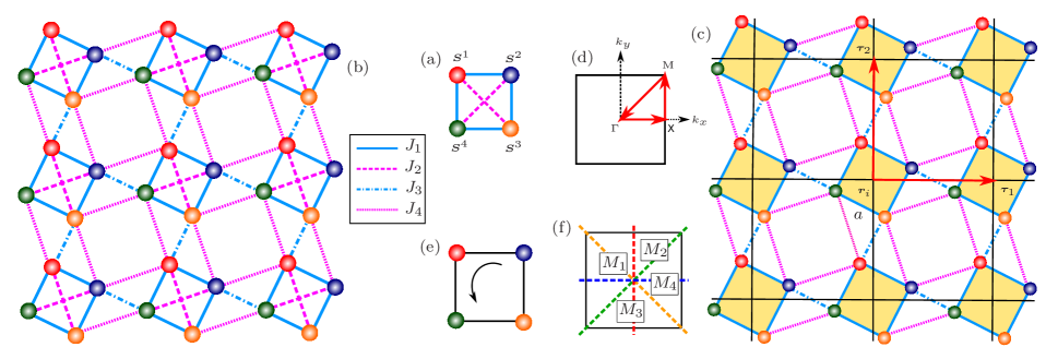
Figure 1: (a) Geometrical view of the square plaquette, (b) $J_{1}$-$J_{2}$-$J_{3}$-$J_{4}$ AFM Heisenberg model on the CaVO lattice, (c) effective square lattice constituted by the smallest square plaquettes, (d) BZ of the square lattice as shown in (c), whose corners are defined by $\Gamma=(0,0)$, X$=(\frac{\pi}{\sqrt{5}\,a},0)$ and M$=(\frac{\pi}{\sqrt{5}\,a},\frac{\pi}{\sqrt{5}\,a})$, (e) system remains invariant under rotation by $\pi/2$ , (f) mirror planes are shown by four different dashed lines.

In this investigation, POT has been developed on an expanded basis space spanned by two singlets and three triplet plaquette states and when the system is studied in terms of weakly interacting plaquettes by means of stronger NN intra-plaquette terms in the Hamiltonian. In another case, bond operator theory (BOT) has been formulated for the system of weakly interacting bonds when the NN inter-plaquette terms in the Hamiltonian are dominant. Obviously, POT and BOT are based on the two different ground states, known as PRVB and dimerized states. Emergence of a variety of nodal-lines is found in the triplet dispersion bands both for plaquette and bond excitations obtained in POT and BOT, respectively, for the frustrated spin-1/2 AFM Heisenberg model on the CaVO lattice.

A pair of six-fold degenerate nodal-loops of different topological features emerges in the plaquette excitations, each of which is found to decouple into three two-fold degenerate loops in the presence of an external magnetic field. This implies the fact that every triplet dispersion branch was triply degenerate due to SU(2) invariance and this degeneracy is withdrawn as soon as the magnetic field is switched on. Among the two loops, one is circular and it is found to appear at a definite energy, while the second one is a square and it is spanned over a finite energy width. One of the decoupled loops for every case is found to appear at the same energy values, while the remaining two are found to shift their positions towards higher energies with the increase of magnetic field. But their overall features remain unaltered under the variation of magnetic field. Thus these nodal-lines are protected by the ${\cal P}$ and U(1) symmetries, since the ${\cal T}$ symmetry is broken by the magnetic field. In case of BOT, system is found to host magnetic field induced multiple nodal-lines of various shapes within the two lower bands of triplon excitations, with the variations of exchange parameters. None of the nodal-lines are four-fold degenerate. So, the system is found to host several non-Dirac nodal-lines, and they seem to be detectable in the inelastic neutron scattering experiment on the frustrated antiferromagnetic compound, CaV₄O₉, under magnetic field.

The article is arranged in the following manner. Section II contains the details of POT. Properties of nodal-lines have been described and effect of magnetic field has been investigated. Similarly, BOT has been described in the section III. Emergence of nodal-lines under the magnetic field has been studied. Summary of the results are presented in the last section (IV).

II Four-spin plaquette operator theory

In order to develop the four-spin POT applicable for the AFM model on CaVO lattice, spin-1/2 operators on the four different vertices of the square plaquette have been expressed in terms of the plaquette operators. Thus, the $\alpha$-th components of the spin operators at the $n$-th vertex, $S^{n}_{\alpha}$, $n=1,2,3,4$, $\alpha=x,y,z$, have been expressed in terms of the basis states spanned by the complete set of eigenstates of a single frustrated square plaquette $\ket{\eta}$ and $\ket{\xi}$ by following the formula $S^{n}_{\alpha}=\langle\eta|S^{n}_{\alpha}|\xi\rangle\ket{\eta}\bra{\xi}$, where summation over repeated indices is assumed Sachdev2 . For this purpose, expressions of the eigenstates of a single frustrated square plaquette are obtained.

II.1 Single square plaquette

The spin-1/2 AFM Heisenberg Hamiltonian on a single square plaquette is defined by

$$H_{\text{\Square}}=\!\sum\limits_{n=1}^{4}\left(J_{1}\,\bm{S}^{n}\cdot\bm{S}^{n+1}\!+\!J_{2}\,\bm{S}^{n}\cdot\bm{S}^{n+2}\right),\,\bm{S}^{n+4}\!=\!\bm{S}^{n},$$ (1)

where $\bm{S}^{n}$ is the spin-1/2 operator at the position $n$. $J_{1}$ and $J_{2}$ are the intra-plaquette NN and NNN exchange interaction strengths, respectively. A pictorial view of this spin model is shown in Fig 1 (a). Non-zero values of $J_{2}$ invokes frustration in this model since the NNN bonds now are not energetically favorable in order to the minimized value of classical ground state energy with respect to the NN bonds. The Hilbert space of this Hamiltonian comprises of 16 states with two singlets ($S_{\rm T}=0$), three triplets ($S_{\rm T}=1$) and one quintet ($S_{\rm T}=2$), where $\bm{S}_{\rm T}=\sum_{n=1}^{4}\bm{S}^{n}$ is the total spin of the plaquette. Two singlets are specified by $\ket{s_{1}}$ and $\ket{s_{2}}$, which can be expressed as linear combinations of two different plaquette states, where each plaquette state is composed of two singlet dimers. In analogy with the conventional pair of bonding and anti-bonding states, these singlet pair can be termed as resonating-valence-bond (RVB) and anti-RVB (aRVB) states. Forms of the wavefunctions, $\Psi_{\rm RVB}\;(\ket{s_{1}})$ and $\Psi_{\rm aRVB}\;(\ket{s_{2}})$ are shown in Fig 2.

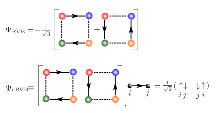
Figure 2: Schematic representation of $\Psi_{\rm RVB}$ and $\Psi_{\rm aRVB}$. Arrow on the NN bonds indicates the spin ordering in singlet dimers.

The exact analytic expressions of all energy eigenstates along with their symmetries have been presented in the Appendix A. Variations of all eigenenergies are shown in Fig 3 for $0<J_{2}/J_{1}<2$, where few crossovers are noted. $E_{s_{1}}$ ($E_{s_{2}}$) is the energy of the singlet state $\ket{s_{1}}$ ($\ket{s_{2}}$), while $E_{t_{1}}=E_{t_{2}}$ and $E_{t_{3}}$ are the energies of the degenerate triplet states $\ket{t_{1,\alpha}}$, $\ket{t_{2,\alpha}}$ and $\ket{t_{3,\alpha}}$, respectively. Quintet has the highest energy, $E_{q}$, for the entire region, $0<J_{2}/J_{1}<2$, so, it does not cross others. Ground state is always a total spin singlet but not unique in the entire parameter regime, as $\ket{s_{1}}$ and $\ket{s_{2}}$ are the ground states in two separate regions, R₁ ($J_{2}<J_{1}$) and R₂ ($J_{2}>J_{1}$), respectively. So, ground state is doubly degenerate at the point, $J_{2}/J_{1}=1$. This indicates the fact that, in contrast to the property of conventional bonding and anti-bonding states, $\Psi_{\rm RVB}$ does not always have energy lower than $\Psi_{\rm aRVB}$. Fig 3 reveals that two different kinds of spin gap occurs for a single square plaquette. One among them can be defined as triplet gap as it corresponds to singlet-triplet transition when $J_{2}/J_{1}<1/4$, while singlet gap (singlet-singlet transition) is found when $J_{2}/J_{1}>1/4$.

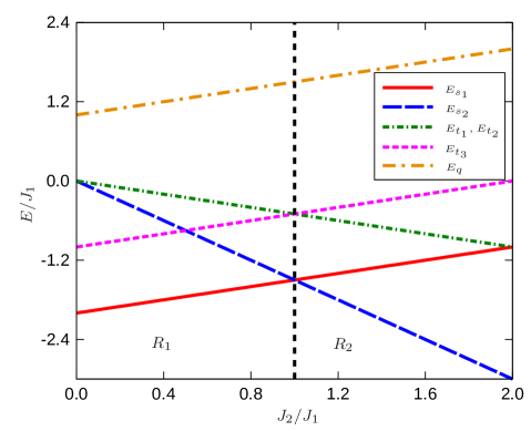
Figure 3: Variation of energy eigenvalues of single plaquette with $J_{2}/J_{1}$. Vertical dashed line separates the two regions, R₁ and R₂.

II.2 Four-spin plaquette operators

The form of spin-1/2 operators expressed in the truncated basis constituted by the lowest singlet and triplet plaquette states is used before for the estimation of PRVB ground state energy ($E_{\rm G}$) and triplet spin gap ($\Delta$) of the CaVO lattice Ueda . The representation of spin-1/2 operators expressed in the basis constituted by the complete set of plaquette eigenstates is available Doretto . Spin-1/2 operators in terms of the all singlet and triplet states had been employed before for finding the $E_{\rm G}$ and $\Delta$ for the four-spin PVBS state of the square lattice Doretto . It is worth mentioning at this time that PRVB ground state is unique and it does not break the symmetry of the CaVO lattice, while the PVBS state is four-fold degenerate and breaks the full translation symmetry of the square lattice Zhitomirsky ; Sachdev1 .

Neglecting the contribution of higher energy quintet states the spin operators, $S^{n}_{\alpha}$, are expressed as,

$$S^{n}_{\alpha}= A^{n}_{a}\left(t^{\dagger}_{a,\alpha}\,s_{1}+s^{\dagger}_{1}t_{a,\alpha}\right)+B^{n}_{a}\left(t^{\dagger}_{a,\alpha}\,s_{2}+s^{\dagger}_{2}\,t_{a,\alpha}\right)$$ (2)

$$+i\,\epsilon_{\alpha\beta\gamma}\,D^{n}_{ab}\,t^{\dagger}_{a,\beta}\,t_{b,\gamma}.$$

Here, $\epsilon_{\alpha\beta\gamma}$ is the antisymmetric Levi-Civita symbol with $\epsilon_{xyz}=1$, and $a,\,b=1,2,3$. The matrix elements, $A^{n}_{a}=\langle s_{1}|S^{n}_{\alpha}|t_{a,\alpha}\rangle$, $B^{n}_{a}=\langle s_{2}|S^{n}_{\alpha}|t_{a,\alpha}\rangle$, and $D^{n}_{ab}=\langle t_{a,\beta}|S^{n}_{\alpha}|t_{b,\gamma}\rangle$, are given in the Appendix A. The vacuum $\ket{0}$ and five plaquette operators are defined here which yield the five physical states $\ket{s_{j}}=s^{\dagger}_{j}\ket{0},\ket{t_{a,\alpha}}=t^{\dagger}_{a,\alpha}\ket{0}$, where $j=1,2$ and $a=1,2,3$. Plaquette operators obey bosonic commutation relations. The completeness relation in the truncated Hilbert space reads as,

$$\sum_{j=1,2}s^{\dagger}_{j}\,s_{j}+\sum_{a,\alpha}t^{\dagger}_{a,\alpha}\,t_{a,\alpha}=1.$$ (3)

The Hamiltonian of a single plaquette, Eq 1, in the same Hilbert space assumes the form

$$H_{\text{\Square}} =\sum_{\begin{subarray}{c}j\end{subarray}}E_{s_{j}}s^{\dagger}_{j}\,s_{j}+\sum_{\begin{subarray}{c}a,\alpha\end{subarray}}E_{t_{a}}\,t^{\dagger}_{a,\alpha}\,t_{a,\alpha}.$$ (4)

II.3 Hamiltonian in terms of plaquette operators

In order to obtain the values of $E_{\rm G}$ and $\Delta$ for the PRVB phase as well as the triplet dispersion bands for the fully frustrated spin-1/2 AFM Heisenberg model on the CaVO lattice, the following Hamiltonian has been considered.

$$H\!\!= \sum\limits_{i}\!\big{[}H_{\text{\Square}}(\bm{r}_{i})\!+\!J_{3}\!\left(\bm{S}^{2}_{\bm{r}_{i}}\!\!\cdot\!\bm{S}^{4}_{\bm{r}_{i}+\bm{\tau}_{1}}\!\!+\!\bm{S}^{1}_{\bm{r}_{i}}\!\!\cdot\!\bm{S}^{3}_{\bm{r}_{i}+\bm{\tau}_{2}}\right)\!\!+\!\!J_{4}\!\big{(}\bm{S}^{2}_{\bm{r}_{i}}\!\!\cdot\!\bm{S}^{1}_{\bm{r}_{i}+\bm{\tau}_{1}}\!$$ (5)

$$+\!\bm{S}^{3}_{\bm{r}_{i}}\!\!\cdot\!\bm{S}^{4}_{\bm{r}_{i}+\bm{\tau}_{1}}+\bm{S}^{2}_{\bm{r}_{i}}\!\!\cdot\!\bm{S}^{3}_{\bm{r}_{i}+\bm{\tau}_{2}}\!+\!\bm{S}^{1}_{\bm{r}_{i}}\!\!\cdot\!\bm{S}^{4}_{\bm{r}_{i}+\bm{\tau}_{2}}\big{)}\big{]}.$$

$J_{3}$ and $J_{4}$ are the inter-plaquette NN and NNN exchange interaction strengths, respectively. Here, the vector $\bm{r}_{i}$ denotes the position of the $i$-th plaquette while $\bm{\tau}_{1}=\sqrt{5}\,a\,\hat{x}$ and $\bm{\tau}_{2}=\sqrt{5}\,a\,\hat{y}$ are the primitive vectors of the effective square lattice formed by the square plaquettes. Here $a$ is the NN lattice spacing of the original CaVO lattice which has been assumed henceforth unity. POT is valid as long as intra-plaquette interactions are stronger than respective inter-plaquette interactions, i. e., $J_{1}>J_{3}$ and $J_{2}>J_{4}$. Here the system is studied in a wider parameter regime, $0<J_{2}/J_{1}<2$, in comparison to all the previous studies where this regime was limited to $0<J_{2}/J_{1}<1$. However, in this case, system is studied in terms of weakly interacting square plaquettes. In other case, BOT is valid for the opposite limit, $J_{1}<J_{3}$, which will be described in the next section.

The plaquette-operator representation (Eq 2) has been substituted in Eq 5 to express the Hamiltonian in terms of the plaquette operators,

$${\cal H}\!=\!E_{0}\!+\!H_{02}\!+\!H_{20}\!+\!H_{30}\!+\!H_{21}\!+\!H_{40}\!+\!H_{22},$$ (6)

where $E_{0}$ is a constant. In $H_{nm}$, $n$ and $m$ indicate the number of triplet and singlet operators, whose explicit forms are given in the Appendix A. The effect of the constraint (Eq 3) has been taken into account by including the following term to the Hamiltonian (Eq 6),

$$-\mu\sum\limits_{i}\bigg{(}\sum\limits_{j=1,2}s^{\dagger}_{j,i}\,s_{j,i}+\sum\limits_{a,\alpha}t^{\dagger}_{a,i,\alpha}\,t_{a,i,\alpha}-1\bigg{)},$$ (7)

where $\mu$ is the Lagrange multiplier. To execute plaquette operator formalism, the lowest-energy singlet is assumed to be condensed and has to be replaced by a number in Eq 6. It is worthy to mention at this point that $\ket{s_{1}}$ and $\ket{s_{2}}$ are the lowest energy singlets in the regions, R₁ and R₂, respectively. The condensation is implemented by making the accompanying substitution, $s^{\dagger}_{j,i}=s_{j,i}=\langle s^{\dagger}_{j,i}\rangle=\langle s_{j,i}\rangle=\bar{s}$ Sachdev2 . The lowest singlet in the respective region has been condensed, which implies that $\ket{s_{j}}$ is condensed in the region R_j, where $j=1,2$. Now the value of the constant, $E_{0}$ is given by the equation, $E_{0}=N\left[\bar{s}^{2}E-\mu\left(\bar{s}^{2}-1\right)\right]$, in which $E=E_{s_{1}}$ ($E_{s_{2}}$) for the region R₁ (R₂) and $N$ is the total number of plaquettes in the system. By assuming the periodic boundary condition, Fourier transformations of the operators $t^{\dagger}_{a,i,\alpha}$ and $s^{\dagger}_{j,i}$ are obtained as,

$$t^{\dagger}_{a,i,\alpha} =\frac{1}{\sqrt{N}}\sum\limits_{\mathbb{k}}\text{exp}\left(-i\mathbb{k}\cdot\bm{R}_{i}\right)t^{\dagger}_{a,\mathbb{k},\alpha},$$ (8)

$$s^{\dagger}_{j,i} =\frac{1}{\sqrt{N}}\sum\limits_{\mathbb{k}}\text{exp}\left(-i\mathbb{k}\cdot\bm{R}_{i}\right)s^{\dagger}_{j,\mathbb{k}},$$

where $j=1,2$ and $a=1,2,3$. Here the momentum sum runs over the BZ of the square lattice, which is shown in Fig 1 (d).

II.4 Quadratic approximation

Henceforth, the system has been studied in terms of an effective boson model where the Hamiltonian keeps only those terms which are quadratic in bosonic plaquette operators. Terms containing more than two plaquette operators, $H_{30},H_{21},H_{40}$ and $H_{22}$, therefore, have been neglected. So, the approximated Hamiltonian becomes,

$${\cal H}_{\rm Q}=E_{0}+H_{02}+H_{20}.$$

In the momentum space it becomes

$${\cal H}_{\rm Q} = \sum\limits_{\mathbb{k}}\left(E_{s_{j}}-\mu\right)s^{\dagger}_{j,\mathbb{k}}s_{j,\mathbb{k}}+\sum\limits_{\mathbb{k}}X^{ab}_{\mathbb{k}}\;t^{\dagger}_{a,\mathbb{k},\alpha}t_{b,\mathbb{k},\alpha}$$ (9)

$$+ \frac{Y^{ab}_{\mathbb{k}}}{2}\!\left(t^{\dagger}_{a,\mathbb{k},\alpha}t^{\dagger}_{b,-\mathbb{k},\alpha}+t_{a,-\mathbb{k},\alpha}t_{b,\mathbb{k},\alpha}\!\right),$$

with $j=2\,(1)$ for the region R₁ (R₂), $a,b=1,2,3$ and $\alpha,\beta,\gamma=x,y,z$. Expressions of the coefficients $X^{ab}_{\mathbb{k}}$ and $Y^{ab}_{\mathbb{k}}$ are given in Appendix A. Singlet sector is diagonalized separately with singlet energies $\Omega_{s_{j}}=\left(E_{s_{j}}-\mu\right)$. The six-component vector $\Psi^{\dagger}_{\mathbb{k},\alpha}=\left(t^{\dagger}_{1,\mathbb{k},\alpha}t^{\dagger}_{2,\mathbb{k},\alpha}t^{\dagger}_{3,\mathbb{k},\alpha}t_{1,\mathbb{-k},\alpha}t_{2,\mathbb{-k},\alpha}t_{3,\mathbb{-k},\alpha}\right)$ is introduced for the diagonalization of the triplet sector. Eq 9 becomes

$${\cal H}_{\rm Q}=E^{\prime}_{0}+\sum\limits_{\mathbb{k}}\left(E_{s_{j}}-\mu\right)s^{\dagger}_{j,\mathbb{k}}s_{j,\mathbb{k}}+\frac{1}{2}\sum\limits_{\mathbb{k}}\Psi^{\dagger}_{\mathbb{k},\alpha}{H_{\mathbb{k}}}\Psi_{\mathbb{k},\alpha},$$

where

$$E^{\prime}_{0}=E_{0}-\frac{3}{2}\sum\limits_{\mathbb{k}}\;\sum_{\begin{subarray}{c}a=1,2,3\end{subarray}}X^{aa}_{\mathbb{k}},\;{\rm and}\;{H_{\mathbb{k}}}=\left({\begin{array}[]{cc}{X_{\mathbb{k}}}&{Y_{\mathbb{k}}}\\ {Y_{\mathbb{k}}}&{X_{\mathbb{k}}}\\ \end{array}}\right).$$ (10)

${X_{\mathbb{k}}}$ and ${Y_{\mathbb{k}}}$ are two different $3\times 3$ hermitian matrices having elements $X^{ab}_{\mathbb{k}}$ and $Y^{ab}_{\mathbb{k}}$, respectively. After diagonalization the Hamiltonian assumes the form

$${\cal H}_{\rm Q}=E_{\rm G}+\sum\limits_{\mathbb{k}}\left(E_{s_{j}}-\mu\right)s^{\dagger}_{j,\mathbb{k}}s_{j,\mathbb{k}}+\frac{1}{2}\sum\limits_{\mathbb{k}}\Phi^{\dagger}_{\mathbb{k},\alpha}{H^{\prime}_{\mathbb{k}}}\Phi_{\mathbb{k},\alpha},$$

with the energy of the PRVB (ground) state

$$E_{\rm G}=E_{0}+\frac{3}{2}\sum\limits_{a,\mathbb{k}}\left(\Omega_{a,\mathbb{k}}-X^{aa}_{\mathbb{k}}\right),$$ (11)

and ${H^{\prime}_{\mathbb{k}}}$ = Diag $[h_{\mathbb{k}},-h_{\mathbb{k}}]_{(2\times 2)}$, where $h_{\mathbb{k}}$ = Diag $[\Omega_{1,\mathbb{k}},\Omega_{2,\mathbb{k}},\Omega_{3,\mathbb{k}}]_{(3\times 3)}$. The eigenvectors $\Phi^{\dagger}_{\mathbb{k},\alpha}$ is given by $\Phi^{\dagger}_{\mathbb{k},\alpha}=\left(b^{\dagger}_{1,\mathbb{k},\alpha}b^{\dagger}_{2,\mathbb{k},\alpha}b^{\dagger}_{3,\mathbb{k},\alpha}b_{1,\mathbb{-k},\alpha}b_{2,\mathbb{-k},\alpha}b_{3,\mathbb{-k},\alpha}\right)$. Relation between the vectors, $\Psi^{\dagger}_{\mathbb{k},\alpha}$ and $\Phi^{\dagger}_{\mathbb{k},\alpha}$ is established by the transformation,

$$\Phi_{\mathbb{k},\alpha}=M_{\mathbb{k}}\Psi_{\mathbb{k},\alpha},\quad{\rm where}\quad M_{\mathbb{k}}=\left({\begin{array}[]{cc}{U^{\dagger}_{\mathbb{k}}}&{-V^{\dagger}_{\mathbb{k}}}\\ {-V^{\dagger}_{\mathbb{k}}}&{U^{\dagger}_{\mathbb{k}}}\\ \end{array}}\right).$$

${U^{\dagger}_{\mathbb{k}}}$ and ${V^{\dagger}_{\mathbb{k}}}$ are two $3\times 3$ hermitian matrices whose elements are the Bogoliubov coefficients $u^{ab}_{\mathbb{k}}$ and $v^{ab}_{\mathbb{k}}$, respectively. The analytic expressions of the triplet excitation energies $\Omega_{a,\mathbb{k}}$, along with $u^{ab}_{\mathbb{k}}$ and $v^{ab}_{\mathbb{k}}$ in terms of the $X^{ab}_{\mathbb{k}}$ and $Y^{ab}_{\mathbb{k}}$ are available in Appendix A. The values of $\mu$ and $\bar{s}^{2}$ are determined by minimizing the ground state energy with respect to themselves, i. e., $\frac{\partial E_{\rm{G}}}{\partial\bar{s}^{2}}=0$ and $\frac{\partial E_{\rm{G}}}{\partial\mu}=0$, which gives

$$\mu=E+\frac{3}{2N}\sum\limits_{a,\mathbb{k}}\left[\frac{\partial\Omega_{a,\mathbb{k}}}{\partial\bar{s}^{2}}-\frac{Y^{aa}_{\mathbb{k}}}{\bar{s}^{2}}\right],$$ (12)

$$\bar{s}^{2}=1+\frac{3}{2N}\sum\limits_{a,\mathbb{k}}\left[\frac{\partial\Omega_{a,\mathbb{k}}}{\partial\mu}+1\right].$$

Singlet, $\Omega_{s_{j}}=E_{s_{j}}-\mu$ and triplet, $\Omega_{a,\mathbb{k}}$ energies have been determined after finding the values of $\mu$ and $\bar{s}^{2}$ numerically by solving the self-consistent Eq 12. In the absence of inter-plaquette interactions, ($J_{3}=0$, $J_{4}=0$), $\bar{s}^{2}=0$ and $\mu=E$. In this limit, $E_{\rm{G}}=E_{s_{j}}$, the value of ground state energy per plaquette becomes equal to the energy of corresponding lowest singlet state. Variations of ground state energy per plaquette, $E_{\rm G}/NJ_{1}$ with respect to $J_{2}/J_{1}$, when $J_{3}=J_{1}/2$ and $J_{4}=J_{2}/2$ is shown in Fig 5 (a), along with the energy of the lowest singlet plaquette state. $E_{\rm G}/NJ_{1}$ is always lower than the lowest singlet energy. Variation of $E_{\rm G}/NJ_{1}$ with $J_{2}/J_{1}$ shows resemblance with that of plaquette singlet energies as shown in Fig 3, in the respective regions. Although, $E_{s_{1}}$ and $E_{s_{2}}$ meet at $J_{2}/J_{1}=1$ (Fig 3), $E_{\rm G}/NJ_{1}$s of the two PRVB states based on the singlets $\ket{s_{1}}$ and $\ket{s_{2}}$ for the respective regions, R₁ and R₂ are found to meet at $J_{2}/J_{1}=0.96$ (Fig 5 (a)) due to the inter-plaquette interactions. This meeting point must vary with the values of $J_{3}$ and $J_{4}$.

The value of $E_{\rm G}$ is further obtained by the second-order perturbative calculation. In this formulation, $H_{0}=\sum_{i=1}^{N}H_{\text{\Square}}(\bm{r}_{i})$, has been treated as the unperturbed Hamiltonian, where $H-H_{0}$ is the perturbation. Here, $H_{0}$ means the sum of all plaquette Hamiltonians, while $H-H_{0}$ implies the sum of all inter-plaquette interactions. Obviously, this result is acceptable as long as intra-plaquette interaction strengths are dominant. The ground state energy per plaquette for the regions R₁ and R₂ has been obtained, where,

$$E^{\rm P}_{\rm G}(\rm R_{1}) =\Big{(}-2J_{1}+J^{\prime}_{2}+6\frac{(\frac{J_{3}+J^{\prime}_{2}}{12})^{2}}{-4J_{1}+2J_{2}}$$ (13)

$$-3\frac{(\frac{J_{3}+J^{\prime}_{2}-2J_{4}}{3})^{2}}{2J_{1}}+6\frac{(\frac{J_{3}+J^{\prime}_{2}}{6\sqrt{2}})^{2}}{-3J_{1}+J_{2}}\Big{)},$$

$$E^{\rm P}_{\rm G}(\rm R_{2}) =\Big{(}-3J^{\prime}_{2}-3\frac{(\frac{J_{3}+J^{\prime}_{2}}{4})^{2}}{J_{2}}\Big{)},$$

with $J^{\prime}_{2}=J_{2}/2$. Variation of $E^{\rm P}_{\rm G}/NJ_{1}$ with $J_{2}/J_{1}$ has been shown by dashed (blue) line in Fig 5 (a), which is found to agree with that obtained in POT shown by red line.

Triplet dispersions as shown in the Figs 7, 9 reveal that value of $\Omega_{3,\mathbb{k}}$ is always the lowest. In addition, its minima occur at the high-symmetry points, $\Gamma$, M and X in the BZ, depending on the values of $J_{2}/J_{1}$, which is shown in Fig 4, where variations of $\Omega_{3,\Gamma}$, $\Omega_{3,{\rm M}}$ and $\Omega_{3,{\rm X}}$ have been plotted with respect to $J_{2}/J_{1}$.

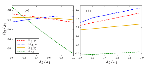
Figure 4: Variation of energies of $\Omega_{3,\Gamma}$, $\Omega_{3,{\rm M}}$ and $\Omega_{3,{\rm X}}$ measured with respect to $E_{\rm G}$ against $J_{2}/J_{1}$ (a) in region R₁, (b) in region R₂, when $J_{3}=J_{1}/2$ and $J_{4}=J_{2}/2$.

In order to estimate the magnitude of $\Delta$, values of $\Omega_{3,\Gamma}$, $\Omega_{3,{\rm M}}$ and $\Omega_{3,{\rm X}}$ are measured with respect to $E_{\rm{G}}$ in Figs 4 (a) and (b), for the regions R₁ and R₂, respectively, where $J_{3}=J_{1}/2$ and $J_{4}=J_{2}/2$. Singlet excitation, $\Omega_{s_{2}}$ in R₁ or $\Omega_{s_{1}}$ in R₂ is always dispersionless in the quadratic approximation irrespective of the values of $J$s. $\Omega_{3,\Gamma}$, $\Omega_{3,{\rm M}}$ and $\Omega_{3,{\rm X}}$ cross each other at a single point, $J_{2}/J_{1}=1/2$ in R₁, as a special case when $J_{3}=J_{1}/2$ and $J_{4}=J_{2}/2$. It means that $\Omega_{3}$ at the points $\Gamma$, M and X has the same value. The plot shows that $\Omega_{3,{\rm M}}$ is the lowest when $J_{2}/J_{1}<1/2$ while $\Omega_{3,\Gamma}$ is that when $J_{2}/J_{1}>1/2$ in R₁. For different values of $J_{3}$ and $J_{4}$, $\Omega_{3,\Gamma}$, $\Omega_{3,{\rm M}}$ and $\Omega_{3,{\rm X}}$ cross each other at different points. On the other hand, $\Omega_{3,{\rm X}}$ is always the lowest in R₂. Ultimately, the value of $\Delta$ has been estimated form this comparative study.

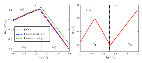
Figure 5: Variations of ground state energy per plaquette (a) and spin gap (b) against $J_{2}/J_{1}$, when $J_{3}=J_{1}/2$ and $J_{4}=J_{2}/2$.

Variations of $\Delta$ with respect to $J_{2}/J_{1}$, when $J_{3}=J_{1}/2$ and $J_{4}=J_{2}/2$ is shown in Fig 5 (b).

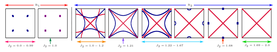
Figure 6: Kaleidoscopic views of the emergent topological nodes and nodal-lines on the BZ with the change of $J_{2}/J_{1}$, covering both the regions R₁ and R₂, when $J_{3}=J_{1}/2$ and $J_{4}=J_{2}/2$.

II.5 Triplet plaquette dispersions

Now, emergence and evolution of topological nodes and nodal-lines will be described in great detail for the two different regions. For this purpose, the triplet dispersion bands, $\Omega_{a,\mathbb{k}}/J_{1}$, $a=1,2,3$, have been shown in Figs 7 (a)-(b) and Figs 9 (a)-(e), for the regions R₁ and R₂, respectively. The dispersions are shown in three-dimensional (3D) plots covering the full BZ, as well as, along the high-symmetry pathway $(\Gamma$,X,M,$\Gamma)$ for every case. Density of states (DOS) is shown in the side panel. Two types of band-touching points or nodes, are found depending on the number of bands at the touching point. They are termed as two-band (2BTP) and three-band touching point (3BTP), where two and three bands are found to meet, respectively. Two kinds of 3BTP are identified owing to their dissimilar nature of dispersion relation around the respective meeting points. Emergence and evolution of those nodes and nodal-lines with the variation of $J_{2}/J_{1}$ have been clearly shown in Fig 6. 2BTP and 3BTP appear both in the regions R₁ and R₂, whereas, nodal-line and flat-band appear only in region R₂.

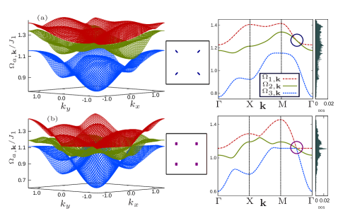
Figure 7: Triplet dispersion bands in R₁ when $J_{2}/J_{1}=0.8$, (a) 1.0, (b), for $J_{3}=J_{1}/2$ and $J_{4}=J_{2}/2$.

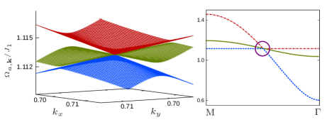
Figure 8: Closer view of triplet dispersions around the 3BTP for $J_{2}/J_{1}=1$ in R₁.

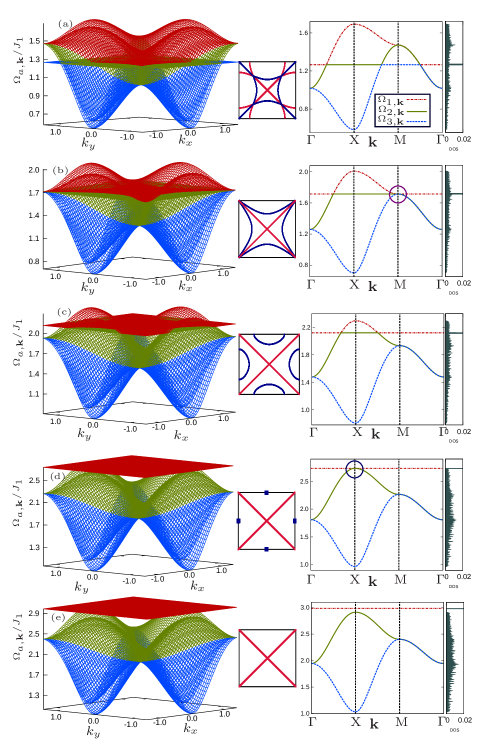
Figure 9: Triplet dispersion in R₂ with $J_{2}/J_{1}$, (a) 1.0, (b) 1.21, (c) 1.4, (d) 1.68, (e) 1.8. Here $J_{3}=J_{1}/2$ and $J_{4}=J_{2}/2$.

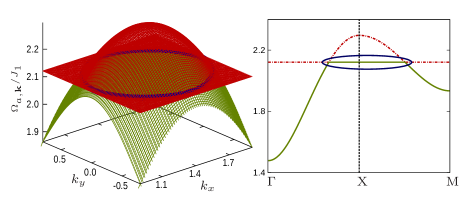
Figure 10: Closer view of triplet excitations around the circular nodal-line for $J_{2}/J_{1}=1.4$.

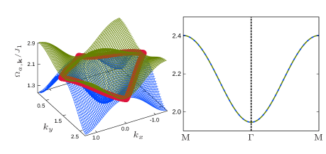
Figure 11: Closer view of triplet excitations around the square nodal-line for $J_{2}/J_{1}=1.8$.

In R₁, a 2BTP in the upper two bands is noted around the point $(\pi/2\sqrt{5},\pi/2\sqrt{5})$ in the BZ, as long as $0\leq J_{2}/J_{1}<1$, which is shown by blue diamond in Fig 7 (a). This 2BTP is replaced by a 3BTP, when $J_{2}/J_{1}=1$, as shown by purple square in Fig 7 (b). They do not therefore coexist. All the 2BTP and 3BTP are shown by open circles along the $(\Gamma$,X,M,$\Gamma)$ pathway. Closer view of triplet dispersions around this 3BTP is shown in Fig 8.

The system in region R₂ hosts two concentric nodal loops with different shapes. They are centered around the X point of the BZ. Among them one is perfectly square and it forms between the lower two bands. Area of the square is exactly equal to the area of the BZ, since it passes through the high-symmetry points, $\Gamma$, M, centering the X. The shape, position and area of this nodal-loop remain unchanged regardless the values of $J_{2}/J_{1}$ for the entire region R₂. Thus, it seems that it is additionally protected by some intrinsic symmetry of the system. The other loop is found between the upper two bands and it appears exactly circular when $J_{2}/J_{1}=1.4$. The area of this loop is always less than that of the BZ. With the increase of $J_{2}/J_{1}$, radius of this loop decreases and becomes a point giving rise to a 2BTP, when $J_{2}/J_{1}=1.68$. The bands get separated by leaving a gap with the further increase of $J_{2}/J_{1}$ beyond the value 1.68. Thus, this loop is not protected by the intrinsic symmetry of the system. Fig 10 and 11 show the magnified views of those nodal loops. It reveals that circular loop occurs at a definite energy, while the square loop spans over a energy width. The system exhibits a 3BTP at the M point of BZ in this region which occurs at a definite value, $J_{2}/J_{1}=1.21$. Features of the 3BTPs in R₁ and R₂ are different. Further, the topmost band becomes flat for the regime $1.68\leq J_{2}/J_{1}\leq 2$. A sharp peak in the DOS indicates the value of energy of this flat band. Coexistence of 2BTP and 3BTP with the nodal-loops is observed in this region. Non-vanishing DOS in those band-structure reveals that there is no true band gap within those triplet dispersion branches. All the nodes and nodal-lines are protected by the ${\cal PT}$ and SU(2) symmetries, since the Hamiltonian (Eq 5) preserves those symmetries. Also, all of them are six-fold degenerate, since each triplet dispersion is three-fold degenerate because of the SU(2) invariance of the system.

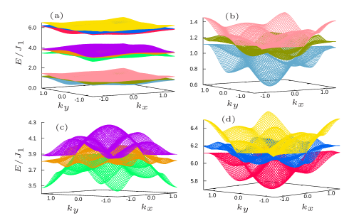
Figure 12: (a) Nine triplet dispersion bands for $h_{z}/J_{1}=3.0$ and $J_{2}/J_{1}=1$ in R₁, when $J_{3}=J_{1}/2$ and $J_{4}=J_{2}/2$. Magnified views of the separated bands are shown in (b), (c) and (d). Higher value of $h_{z}$ is assumed in (a) to show clear separation between the bands although this phenomenon is true for any values of $h_{z}$.

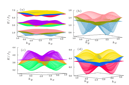
Figure 13: (a) Nine triplet dispersion bands for $h_{z}/J_{1}=3.7$ and $J_{2}/J_{1}=1$ in R₂, when $J_{3}=J_{1}/2$ and $J_{4}=J_{2}/2$. Magnified views of the separated bands are shown in (b), (c) and (d).

II.6 Effect of the magnetic field

The effect of magnetic field on those triplet dispersions has been studied by applying the field along the $\hat{z}$ direction. For this purpose, the Zeeman term, $H_{\rm Z}$, has been added to the Hamiltonian (Eq 5). $H_{\rm Z}=h_{z}\sum_{i=1}^{N}\,S^{z}_{\rm T}(\bm{r}_{i})$, where $h_{z}$ is the strength of the magnetic field and $S^{z}_{\rm T}(\bm{r}_{i})$ is the $z$-component of total spin of the $i$-th plaquette. $H_{\rm Z}$ breaks the ${\cal T}$ and SU(2) symmetries, but preserves the ${\cal P}$ and U(1) symmetries. As a result, the three-fold degeneracy of the triplet states is lost.

In order to obtain the dispersion relations, POT has been developed for the total Hamiltonian, $H_{\rm T}=H\,({\rm Eq}\,\ref{ham1})+H_{\rm Z}$. By expressing $H_{\rm Z}$ in terms of plaquette operators followed by the Fourier transformation, it has the following form in the momentum space,

$${\cal H}_{\rm Z}=ih_{z}\sum_{a,\mathbb{k}}\left(t^{\dagger}_{a,\mathbb{k},x}t_{a,\mathbb{k},y}-t^{\dagger}_{a,\mathbb{k},y}t_{a,\mathbb{k},x}\right).$$ (14)

The singlet plaquette operators, $s_{j,\mathbb{k}}$, do not appear in ${\cal H}_{\rm Z}$, since the energy of singlet states remains unaffected by the presence of magnetic field. As a result, the singlet ground state energy does not depend on it. After the quadratic approximation, the total Hamiltonian becomes ${\cal H}_{\rm T}={\cal H}_{\rm Q}\,({\rm Eq}\,\ref{ham3})+{\cal H}_{\rm Z}$. To perform the Bogoliubov diagonalization, ${\cal H}_{\rm T}$ has been expressed in terms of a eighteen-component vector. Dispersion relations are obtained numerically following the Bogoliubov diagonalization of the 18$\times$18 matrix as described in Appendix A.

Every three-fold degenerate dispersion band has been splitted into three non-degenerate bands in such a fashion that nine bands ultimately form three groups of bands in which each group contains three bands. This is true for each region. Energy gap between the group of bands increases with the increase of $h_{z}$, but without changing the energy of the lowest group of band. So, the value of $\Delta$ does not change with $h_{z}$. These dispersion bands are shown in Figs 12 and 13 for regions R₁ and R₂, respectively. Among the three, the particular group of non-degenerate bands having the lowest energy is identical with the degenerate bands in a sense that feature of each of the three dispersion relation is the same to that when the magnetic field was absent. Other two groups of non-degenerate bands have been shifted towards the higher energies with a little deformation in their dispersion relations. This deformation is perhaps due to the quadratic approximation. These three groups of bands have been depicted separately in Figs 12-13 (b), (c) and (d), for the respective regions. Obviously, the mode of splitting remains the same irrespective of the direction of the applied magnetic field. This splitting is similar to that of a triplet state under the magnetic field with the difference that energy values of the shifted states are not symmetric about that of the $S_{\rm T}^{z}=0$ state. This difference attributes to the fact that triplet states corresponding to $t^{\dagger}_{\alpha}\ket{0},\,\alpha=x,y$, are not the eigenstates of $S_{\rm T}^{z}$. Upon examining the structure of individual group of bands more closely, it reveals that all the respective topological nodes and nodal-loops are there as before when the magnetic field was absent and their features remain unaltered. The features of the nodes and nodal-loops within each group of band is robust against the change of $h_{z}$ and and they cannot be destroyed by increasing the value of $h_{z}$. However, in this case, they are doubly degenerate and protected by both the ${\cal P}$ and U(1) symmetries. So, these loops cannot be termed as Dirac nodal-loops either in the presence or absence of magnetic field.

III Bond operator theory

In this section, BOT has been formulated for the AFM Heisenberg model on the CaVO lattice, where the system is studied in terms of weakly interacting NN bonds connecting the plaquettes. So, in this case, $J_{3}>J_{1}$, and the ground state is composed of singlet dimer on the inter-plaquette NN bonds with strength $J_{3}$. This ground state is known as the dimerized state, whose geometrical view on the CaVO lattice is shown in Fig 14 (a). Values of $E_{\rm G}$ and $\Delta$ of the dimerized state for this model have been determined along with the dispersion of the triplet bond excitation. BOT has been developed by following the formalism introduced before by Sachdev and other in the complete basis space spanned by the singlet, $\ket{s}$, and three triplet states, $\ket{t_{\alpha}},\,\alpha=x,y,z$, on the bond Sachdev2 .

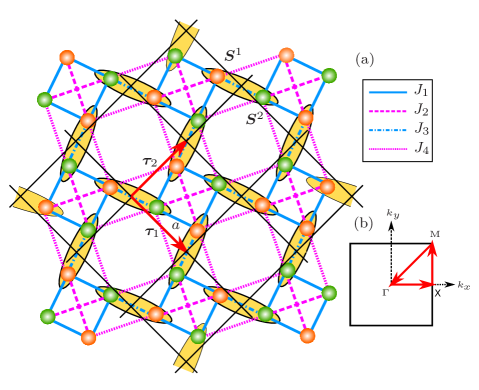
Figure 14: (a) Schematic representation of the dimerized state on the CaVO lattice, where the singlet dimer on the $J_{3}$ bond is shown by the narrow ellipse, (b) BZ of the dimerized lattices defined by $\Gamma=(0,0)$, X$=(\frac{2\pi}{\sqrt{10}a},0)$ and M$=(\frac{2\pi}{\sqrt{10}a},\frac{2\pi}{\sqrt{10}a})$.

The bosonic singlet and triplet creation operators are defined as

$$\ket{s}=s^{\dagger}\ket{0}=\frac{1}{\sqrt{2}}\left(\ket{\uparrow\downarrow}-\ket{\downarrow\uparrow}\right),\;$$ (15)

$$\ket{t_{x}}=t^{\dagger}_{x}\ket{0}=-\frac{1}{\sqrt{2}}\left(\ket{\uparrow\uparrow}-\ket{\downarrow\downarrow}\right),\;$$

$$\ket{t_{y}}=t^{\dagger}_{y}\ket{0}=\frac{i}{\sqrt{2}}\left(\ket{\uparrow\uparrow}+\ket{\downarrow\downarrow}\right),\;$$

$$\ket{t_{z}}=t^{\dagger}_{z}\ket{0}=\frac{1}{\sqrt{2}}\left(\ket{\uparrow\downarrow}+\ket{\downarrow\uparrow}\right).\;$$

The physical constraint considering the completeness relation is

$$s^{\dagger}s+\sum_{\alpha}t^{\dagger}_{\alpha}\,t_{\alpha}=1,$$ (16)

where the Hamiltonian for a single bond assumes the form

$$\bm{S}^{1}\!\cdot\!\bm{S}^{2}=-\frac{3}{4}s^{\dagger}s+\frac{1}{4}t^{\dagger}_{\alpha}\,t_{\alpha}.$$

The spin operators, $S^{n}_{\alpha}$, in terms of the bond operators $s^{\dagger}$ and $t^{\dagger}_{\alpha}$ read as

$$S^{n}_{\alpha}= \frac{(-1)^{n-1}}{2}\left(t^{\dagger}_{\alpha}\,s+s^{\dagger}t_{\alpha}\right)-\frac{i}{2}\,\epsilon_{\alpha\beta\gamma}\,t^{\dagger}_{\beta}\,t_{\gamma}.$$ (17)

Here, $n=1,2$, specifies the positions of two spins in a bond and $\alpha,\beta,\gamma=x,y,z$. The lattice generated by the middle points of every dimer is essentially a square one, whose primitive cell may be constructed by the two primitive vectors, $\bm{\tau}_{1}$ and $\bm{\tau}_{2}$, where $\bm{\tau}_{1}=\frac{\sqrt{10}\,a}{2}\,\hat{x}$, and $\bm{\tau}_{2}=\frac{\sqrt{10}\,a}{2}\,\hat{y}$. Again, $a$ specifies the NN lattice spacing of the CaVO lattice which was assumed before unity. The area of the primitive cell in this case is one-half to the area of that used for developing the POT. So, area of BZ is double to that for the previous case as shown in Fig 14 (b).

The Heisenberg Hamiltonian to formulate the BOT on the CaVO lattice can be written as

$$H^{\prime}\!= \sum\limits_{i}\!\big{[}J_{3}\bm{S}^{1}_{\bm{r}_{i}}\!\cdot\!\bm{S}^{2}_{\bm{r}_{i}}\!+\!J_{1}\!\left(\bm{S}^{2}_{\bm{r}_{i}}\!\cdot\!\bm{S}^{1}_{\bm{r}_{i}+\bm{\tau}_{1}}\!+\bm{S}^{2}_{\bm{r}_{i}}\!\cdot\!\bm{S}^{1}_{\bm{r}_{i}+\bm{\tau}_{2}}\right)+$$ (18)

$$\!J_{4}\!\left(\bm{S}^{2}_{\bm{r}_{i}}\!\cdot\!\bm{S}^{2}_{\bm{r}_{i}+\bm{\tau}_{1}}\!+\bm{S}^{1}_{\bm{r}_{i}}\!\cdot\!\bm{S}^{1}_{\bm{r}_{i}+\bm{\tau}_{2}}\right)+\!J_{2}\bm{S}^{2}_{\bm{r}_{i}}\!\cdot\!\bm{S}^{2}_{\bm{r}_{i}+\bm{\tau}_{1}+\bm{\tau}_{2}}\big{]}.$$

Here, $\bm{S}^{n}_{\bm{r}_{i}}$ is the $n$-th spin of the $i$-th bond. In terms of bond operators, the Hamiltonian looks like

$${\cal H}^{\prime} =H_{1}+H_{2}+H_{3},\;{\rm where}$$ (19)

$$H_{1} =J_{3}\sum\limits_{i}\left(-\frac{3}{4}s^{\dagger}_{\bm{r}_{i}}s_{\bm{r}_{i}}+\frac{1}{4}t^{\dagger}_{\bm{r}_{i},\alpha}t_{\bm{r}_{i},\alpha}\right)$$

$$-\mu\sum\limits_{i}\left(s^{\dagger}_{\bm{r}_{i}}s_{\bm{r}_{i}}+t^{\dagger}_{\bm{r}_{i},\alpha}t_{\bm{r}_{i},\alpha}-1\right),$$

$$H_{2}= \sum\limits_{i,m,\alpha}g(m)\Big{(}t^{\dagger}_{\bm{r}_{i},\alpha}t_{\bm{r}_{i}+\bm{\tau^{\prime}}_{m},\alpha}s^{\dagger}_{\bm{r}_{i}}s_{\bm{r}_{i}+\bm{\tau^{\prime}}_{m}}$$

$$+t^{\dagger}_{\bm{r}_{i},\alpha}t^{\dagger}_{\bm{r}_{i}+\bm{\tau^{\prime}}_{m},\alpha}s_{\bm{r}_{i}}s_{\bm{r}_{i}+\bm{\tau^{\prime}}_{m}}+\mathbb{H.c.}\Big{)},$$

$$H_{3}= \sum\limits_{i,m,\alpha}\epsilon_{\alpha\beta\gamma}\epsilon_{\alpha\beta^{\prime}\gamma^{\prime}}g^{\prime}(m)t^{\dagger}_{\bm{r}_{i},\beta}t^{\dagger}_{\bm{r}_{i},\gamma}t_{\bm{r}_{i}+\bm{\tau^{\prime}}_{m},\beta^{\prime}}t_{\bm{r}_{i}+\bm{\tau^{\prime}}_{m},\gamma^{\prime}},$$

with $m=1,2,3$, $\bm{\tau}^{\prime}_{1}=\bm{\tau}_{1}$, $\bm{\tau}^{\prime}_{2}=\bm{\tau}_{2}$, $\bm{\tau}^{\prime}_{3}=\bm{\tau}_{1}+\bm{\tau}_{2}$, $g(1)=g(2)=-J_{1}/4+J_{4}/4$, $g^{\prime}(1)=g^{\prime}(2)=J_{1}/4+J_{4}/4$, and $g(3)=g^{\prime}(3)=J_{2}/4$. Effect of the constraint, Eq 16, has been taken into account in Eq 19 like before.

III.1 Quadratic and mean-field approximations

In quadratic approximation, contribution of $H_{3}$ is neglected. So, the Hamiltonian in the momentum space is, ${\cal H}^{\prime}_{\rm Q}=E^{\prime}_{0}+H_{2}$, where

$$E^{\prime}_{0}= N^{\prime}\left[-\frac{3}{4}J_{3}\bar{s}^{2}-\mu\left(\bar{s}^{2}-1\right)\right],$$ (20)

$$H_{2}= \sum\limits_{\mathbb{k}}A_{\mathbb{k}}t^{\dagger}_{\mathbb{k},\alpha}t_{\mathbb{k},\alpha}+\frac{B_{\mathbb{k}}}{2}\!\left(t^{\dagger}_{\mathbb{k},\alpha}t^{\dagger}_{-\mathbb{k},\alpha}+t_{-\mathbb{k},\alpha}t_{\mathbb{k},\alpha}\right),$$

with $N^{\prime}=2N$, the total number of dimers in the system and

$$A_{\mathbb{k}} =(\frac{J_{3}}{4}-\mu)+B_{\mathbb{k}},$$

$$B_{\mathbb{k}} =2\,\bar{s}^{2}\sum_{m=1,2,3}g(m)\,\cos\left(\mathbb{k}\cdot\bm{\tau}^{\prime}_{m}\right).$$

Condensation of the singlets is implemented by the substitution, $s^{\dagger}_{\bm{r}_{i}}=s_{\bm{r}_{i}}=\langle s^{\dagger}_{\bm{r}_{i}}\rangle=\langle s_{\bm{r}_{i}}\rangle=\bar{s}$ Sachdev2 . The values of $\mu$ and $\bar{s}^{2}$ are determined by solving the pair of following self-consistent equations.

$$\mu=-\frac{3}{4}J_{3}+\frac{3}{2N^{\prime}}\sum\limits_{\mathbb{k}}\left[\frac{(A_{\mathbb{k}}-B_{\mathbb{k}})}{\Omega_{\mathbb{k}}}-1\right]\frac{B_{\mathbb{k}}}{\bar{s}^{2}},$$ (21)

$$\bar{s}^{2}=1+\frac{3}{2N^{\prime}}\sum\limits_{\mathbb{k}}\left[1-\frac{A_{\mathbb{k}}}{\Omega_{\mathbb{k}}}\right].$$

Diagonalizing the Hamiltonian, $H_{2}$ in Eq 20, by the bosonic Bogoliubov transformation, triplet dispersion is obtained, which is $\Omega_{\mathbb{k}}=\sqrt{A^{2}_{\mathbb{k}}-B^{2}_{\mathbb{k}}}$, along with the ground state energy of the system in BOT, $E^{\prime}_{\rm G}=E^{\prime}_{0}+\frac{3}{2}\sum_{\mathbb{k}}\left(\Omega_{\mathbb{k}}-A_{\mathbb{k}}\right)$.

To obtain more accurate value of $E_{\rm G}$, contribution of the terms containing quartic triplet operators, $H_{3}$ in Eq 19, is taken into account by performing mean-field approximation on them. The terms of cubic order in the triplet operators do not contribute since the condensation of triplet operators is not allowed in this formulation Sachdev2 . By introducing the real space mean-field order parameters, $P(m)=\sum_{\beta}\langle t^{\dagger}_{{\bm{r}_{i}},\beta}t_{{\bm{r}_{i}+\bm{\tau^{\prime}}_{m}},\beta}\rangle$ and $Q(m)=\sum_{\beta}\langle t^{\dagger}_{{\bm{r}_{i}},\beta}t^{\dagger}_{{\bm{r}_{i}+\bm{\tau^{\prime}}_{m}},\beta}\rangle$ with $m=1,2,3$, the mean-field Hamiltonian Susobhan , $H_{\rm MF}$ becomes,

$$H_{\rm MF} =H^{\prime}_{1}+H^{\prime}_{2},\,{\rm with}\;$$ (22)

$$H^{\prime}_{1} =H_{1}+\frac{2}{3}\sum\limits_{m}g^{\prime}(m)\left[Q^{2}(m)-P^{2}(m)\right],$$

$$H^{\prime}_{2} =H_{2}+\frac{2}{3}\,\sum\limits_{i,m}g^{\prime}(m)P(m)\left(t^{\dagger}_{\bm{r}_{i},\alpha}t_{\bm{r}_{i}+\bm{\tau^{\prime}}_{m},\alpha}+\mathbb{H.c.}\right)$$

$$-\frac{2}{3}\,\sum\limits_{i,m}g^{\prime}(m)Q(m)\left(t^{\dagger}_{\bm{r}_{i},\alpha}t^{\dagger}_{\bm{r}_{i}+\bm{\tau^{\prime}}_{m},\alpha}+\mathbb{H.c.}\right).$$

Geometrical symmetries of $\bm{\tau}^{\prime}_{m}$s allow to consider the following relations, $P(1)=P(2)=P_{1}$, $P(3)=P_{2}$, $Q(1)=Q(2)=Q_{1}$ and $Q(3)=Q_{2}$. In the momentum space, $H_{\rm MF}=E^{\prime}_{0}+H^{\prime}_{2}$, where,

$$E^{\prime}_{0}= N^{\prime}\left[-\frac{3}{4}J_{3}\bar{s}^{2}-\mu\left(\bar{s}^{2}-1\right)\!+\!\frac{1}{2}\sum\limits_{j=1,2}r_{j}\left(Q^{2}_{j}-P^{2}_{j}\right)\right],$$ (23)

$$H^{\prime}_{2}= \sum\limits_{\mathbb{k}}A^{\prime}_{\mathbb{k}}t^{\dagger}_{\mathbb{k},\alpha}t_{\mathbb{k},\alpha}+\frac{B^{\prime}_{\mathbb{k}}}{2}\!\left(t^{\dagger}_{\mathbb{k},\alpha}t^{\dagger}_{-\mathbb{k},\alpha}+t_{-\mathbb{k},\alpha}t_{\mathbb{k},\alpha}\!\right),$$

with $r_{1}=4\left(g^{\prime}(1)+g^{\prime}(2)\right)/3$, $r_{2}=4g^{\prime}(3)/3$ and $A^{\prime}_{\mathbb{k}}=A_{\mathbb{k}}+\frac{4}{3}\sum_{m}g^{\prime}(m)P(m)\cos\left(\mathbb{k}\cdot\bm{\tau}^{\prime}_{m}\right)$, $B^{\prime}_{\mathbb{k}}=B_{\mathbb{k}}-\frac{4}{3}\sum_{m}g^{\prime}(m)Q(m)\cos\left(\mathbb{k}\cdot\bm{\tau}^{\prime}_{m}\right)$. Values of the order parameters have been determined by solving two pairs of self-consistent equations,

$$P_{j}=\frac{3}{2}\,\frac{1}{N^{\prime}r_{j}}\sum\limits_{\mathbb{k}}\left[\left(\frac{A^{\prime}_{\mathbb{k}}}{\Omega_{\mathbb{k}}}-1\right)\frac{\partial A^{\prime}_{\mathbb{k}}}{\partial P_{j}}\right],$$ (24)

$$Q_{j}=\frac{3}{2}\,\frac{1}{N^{\prime}r_{j}}\sum\limits_{\mathbb{k}}\left[\frac{B^{\prime}_{\mathbb{k}}}{\Omega_{\mathbb{k}}}\frac{\partial B^{\prime}_{\mathbb{k}}}{\partial Q_{j}}\right],$$

with $j=1,2$, in addition to the equations those are previously obtained for $\mu$ and $\bar{s}^{2}$, in Eq 21. Diagonalizing the Hamiltonian $H^{\prime}_{2}$ like before, the mean-filed dispersion relation, $\Omega^{\prime}_{\mathbb{k}}=\sqrt{A^{\prime 2}_{\mathbb{k}}-B^{\prime 2}_{\mathbb{k}}}$, and the mean-field ground state energy, $E^{\prime\prime}_{\rm G}=E^{\prime}_{0}+\frac{3}{2}\sum_{\mathbb{k}}\left(\Omega^{\prime}_{\mathbb{k}}-A^{\prime}_{\mathbb{k}}\right)$, have been obtained. Ground state energy per bond has been obtained by using the second-order perturbation theory, which has the expression, $E^{\rm P}_{\rm G}=-3J_{3}\left(1+\left((J_{1}-(J_{2}/2)-J_{4})/2\sqrt{2}J_{3}\right)^{2}\right)/4$. However, in this case, the unperturbed Hamiltonian is the sum of all the NN inter-plaquette interactions, $H^{\prime}_{0}=J_{3}\sum_{i=1}^{N^{\prime}}\bm{S}^{1}_{\bm{r}_{i}}\cdot\bm{S}^{2}_{\bm{r}_{i}}$, while the perturbation, $H^{\prime}-H^{\prime}_{0}$, includes all the remaining terms. This result is valid as long as the strengths of NN inter-plaquette interactions are stronger than others.

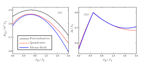
Figure 15: Variation of (a) Ground-state energy per bond and (b) spin gap against $J_{2}/J_{1}$ for $J_{3}=2J_{1}$ and $J_{4}=J_{2}$.

Variation of ground state energy per bond for the regime, $0<J_{2}/J_{1}<2$, obtained in quartic, mean-field and perturbative approximations with respect to $J_{2}/J_{1}$ are shown in Fig 15 (a), for $J_{3}=2J_{1}$ and $J_{4}=J_{2}$. Mean-field estimation, $E^{\prime\prime}_{\rm G}$ is the lowest since it includes the contributions of the quartic terms.

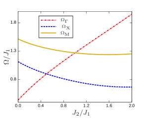
Figure 16: Variation of energies of $\Omega_{\Gamma}$, $\Omega_{{\rm M}}$ and $\Omega_{{\rm X}}$ measured with respect to $E^{\prime}_{\rm G}$ with $J_{2}/J_{1}$, when $J_{3}=2J_{1}$ and $J_{4}=J_{2}$.

In order to estimate the value of $\Delta$, variations of the triplet energies for the high-symmetry points, $\Omega_{\Gamma}$, $\Omega_{{\rm X}}$ and $\Omega_{{\rm M}}$ have been plotted with $J_{2}/J_{1}$, when $J_{3}=2J_{1}$ and $J_{4}=J_{2}$ in Fig 16, as the minima of $\Omega_{\mathbb{k}}$ are found to occur at those points. It shows that $\Omega_{\Gamma}$ and $\Omega_{{\rm X}}$ cross each other at the point $J_{2}/J_{1}=1/2$, in such a way that $\Omega_{\Gamma}$ is the lowest when $J_{2}/J_{1}<1/2$ while $\Omega_{{\rm X}}$ is that when $J_{2}/J_{1}>1/2$. The value of triplet gap, $\Delta$, which accounts the separation between ground and the lowest triplet state energies has been obtained for the regime, $0<J_{2}/J_{1}<2$. Variation of $\Delta$ is shown in Fig 15 (b).

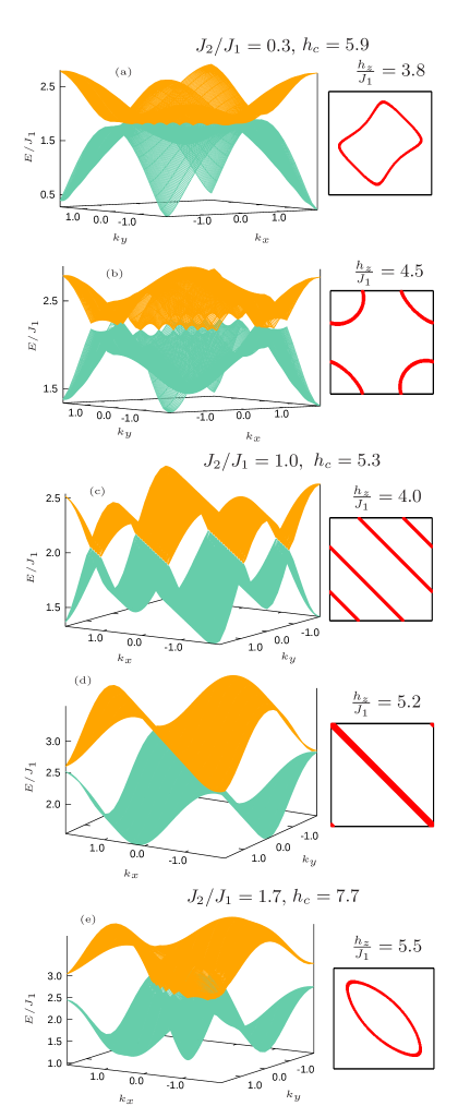
Figure 17: Forms of nodal-loops and nodal-lines for different values of interaction strengths and magnetic fields when $J_{3}=2J_{1}$ and $J_{4}=J_{2}$. The topmost triplon band is not shown as it is clearly separated from the middle band in every case.

To investigate the effect of magnetic field, ${\cal H}^{\prime}_{\rm Z}$ has been added to ${\cal H}^{\prime}$. Expression of ${\cal H}^{\prime}_{\rm Z}$ in terms of triplet operators in the momentum space is, ${\cal H}^{\prime}_{\rm Z}=ih_{z}\sum_{\mathbb{k}}\left(t^{\dagger}_{\mathbb{k},x}t_{\mathbb{k},y}-t^{\dagger}_{\mathbb{k},y}t_{\mathbb{k},x}\right)$, when the magnetic field acts along the $\hat{z}$ direction. Now, the degenerate triplet band splits into three non-degenerate triplon bands and the separation between them increases with the increase of $h_{z}$. They are completely separated from each other above the critical values of magnetic field, $h_{c}$, where the value of $h_{c}$ depends on the values of the exchange parameters. Magnetic field induced nodal-lines of various forms and positions on the BZ are found within the lower triplon dispersion bands, as long as $h_{z}<h_{c}$. For examples, nodal-loops are found when $J_{2}/J_{1}=0.3$ and 1.7, for $J_{3}=2J_{1}$ and $J_{4}=J_{2}$, which are shown in Figs 17 (a), (b) and (e). Elliptic loop is noticed when $J_{2}/J_{1}=1.7$ and $h_{z}/J_{1}<7.7$. Closed loop with various shapes can be obtained for $J_{2}/J_{1}=0.3$ by changing the values of $h_{z}$ as long as $h_{z}/J_{1}<5.9$. Straight nodal-lines are obtained when $J_{2}/J_{1}=1$, for $4.0<h_{z}/J_{1}<5.2$ (Figs 17 (c) and (d)).

So, all of those doubly-degenerate nodal-lines are protected by the ${\cal P}$ and U(1) symmetries. These magnetic field induced nodal-lines do not survive above the $h_{c}$. It is worthy to state that the dimerized ground state is unstable at the higher magnetic field. So the validity of the BOT is questionable in the presence of high magnetic field.

IV Discussion

In this study, emergence of topological nodal-lines with various features has been reported in the frustrated AFM spin-1/2 Heisenberg model formulated on the CaVO lattice. CaVO lattice can be transformed into two different square lattices by treating either four-site plaquettes or two-site bonds as a basis sites as shown in Figs 1 (c) and 14 (a), respectively. POT and BOT have been developed in two different parameter regimes by choosing the values of NN and NNN inter- and intra-plaquette interactions in such a way that the effective Hamiltonians in terms of plaquette and bond operators formulated on the respective square lattices are valid. Dispersion relations of triplet plaquette and bond excitations, based on the PRVB and dimerized ground states are obtained, where nodal-lines are found to exist in the presence and absence of magnetic field. Ground state energy and spin gap in both the regimes have been obtained in this context.

Emergence of a pair of six-fold degenerate nodal-loops with circular and square shapes are noted in the plaquette dispersions, which are ${\cal PT}$ and SU(2) protected. In the presence of magnetic field, three pairs of two-fold degenerate nodal-loops of almost the same features are found, those are ${\cal P}$ and U(1) protected. The system hosts a number of magnetic field induced nodal-lines of various shapes in the triplon dispersions. The system hosts only non-Dirac nodal-lines because of the fact that none of them are four-fold degenerate and protected by the ${\cal PT}$ symmetry. But a pair of Dirac nodal-loops have been noted before in the AFM magnon dispersions for a Heisenberg model on this lattice by considering a larger unit cell containing eight sites Owerre . This difference attributes to the fact that AFM ground state breaks the full symmetry of the Heisenberg Hamiltonian, while the singlet ground states in this study do not. Emergence of multiple topological phases in irradiated tight-binding and FM Kitaev-Heisenberg models on this lattice is noted before Arghya ; Moumita2 . The effect of DMI cannot be registered either in POT or BOT because of the fact that, $\sum_{n}({\bm{S}}^{n}\times{\bm{S}}^{n+1})_{z}$ vanishes identically over a plaquette and bond, when $\bm{S}$ is expressed in terms of either plaquette or bond operators, respectively.

The value of spin-gap for CaV₄O₉ has been determined by measuring the uniform spin susceptibility, and the NMR spin-lattice relaxation rate Taniguchi , as well as by the inelastic neutron scattering Kodama . In the scattering experiment, both powder sample and single crystal of CaV₄O₉ have been used. Both $Q$- and $\theta$-scans have been performed where $Q$ and $\theta$ are the absolute value of scattering wave vector and sample-angle, respectively. For the measurement of spin-gap only the lowest energy dispersion branch has been determined.

However, in order to observe the nodal points and lines, at least a pair of lower energy dispersion branches are to be determined distinctly in the inelastic neutron scattering experiment. For this purpose, wave vector dependent scans on the single crystal would be useful. Repeated scans with varying scattering wave vector in the presence of magnetic field are necessary, however, the direction of the field is irrelevant. BOT predicted several types of nodal-lines (Fig 17) only in the presence of magnetic field, while, POT noted the circular nodal-loop (Fig 10) between two lower bands where those lines occur at a fixed energy. So, scan with fixed incident neutron energy is sufficient for there observation. On the other hand, the square nodal-loop (Fig 11) found in POT occurs between the upper two bands where it is spanned over a finite energy range. Scanning with incident neutrons with a wide range of energies is thus required for its detection.

V ACKNOWLEDGMENTS

MD acknowledges the UGC fellowship, No. 524067 (2014), India.

VI Author contribution statement

MD did both analytical and numerical works as well as prepared the figures. Both the authors were involved in the preparation of the manuscript.

Appendix A Details of plaquette operator theory

A.1 Symmetries of eigenstates of four-spin Heisenberg plaquette

Symmetries of all the eigenvectors of the single square plaquette, $H_{\text{\Square}}$, are described in terms of eight operators of dihedral group $D_{4}$, four rotations, $R_{n}$ and reflections, $M_{n}$, $n=1,2,3,4$. Here, $R$ implies the rotation by $\pi/2$ about the center of the square, as depicted in Fig 1 (e) and $R_{n}$ means successive $R$ operation by $n$ times. Rotation $R$ can be defined as $R\ket{S_{1}S_{2}S_{3}S_{4}}=\ket{S_{2}S_{3}S_{4}S_{1}}$, where $\ket{S_{1}S_{2}S_{3}S_{4}}=\ket{S_{1}^{z}}\otimes\ket{S_{2}^{z}}\otimes\ket{S_{3}^{z}}\otimes\ket{S_{4}^{z}}$, in which $\ket{S_{n}^{z}}$ is the spin state at the $n$-th vertex of the square. Rotational property of an eigenstate, $|\nu\rangle$, can be studied in terms of an eigenvalue equation, $R_{p}|\nu\rangle=\lambda_{r}|\nu\rangle$, where $\lambda_{r}=\pm 1$ be the eigenvalue of the rotational operator $R_{p}$. Where $p<4$ and it corresponds that minimum number of $R$ operations on $|\nu\rangle$ for which $\lambda_{r}$ assumes the value either $+1$ or $-1$. $\lambda_{r}=\pm 1$ imply the even (symmetric) and odd (antisymmetric) parity of the state. Each state has definite parity and among all six are symmetric. It is found that $p$ assumes the value either 1 or 2. For $\Psi_{\rm RVB}$ ($\Psi_{\rm aRVB}$), $\lambda_{r}=1(-1)$ and $p=1$, which means that $\Psi_{\rm RVB}$ is symmetric, whereas, $\Psi_{\rm aRVB}$ is antisymmetric under the rotation by the angle $\pi/2$.

Similarly, reflectional symmetry of $|\nu\rangle$ has been studied in terms of an eigenvalue equation $M_{n}|\nu\rangle=\lambda_{M_{n}}|\nu\rangle$, where four different mirror planes for $M_{n}$ are shown by dashed lines in Fig 1 (f). ${M}_{n}$ are defined as ${M}_{1}\ket{S_{1}S_{2}S_{3}S_{4}}=\ket{S_{1}S_{4}S_{3}S_{2}},\;{M}_{2}\ket{S_{1}S_{2}S_{3}S_{4}}=\ket{S_{3}S_{2}S_{1}S_{4}},\;{M}_{3}\ket{S_{1}S_{2}S_{3}S_{4}}=\ket{S_{2}S_{1}S_{4}S_{3}},\;{M}_{4}\ket{S_{1}S_{2}S_{3}S_{4}}=\ket{S_{4}S_{3}S_{2}S_{1}}$. Values of $\lambda_{M_{3}}$ and $\lambda_{M_{4}}$ remain undefined for the degenerate triplets, $\ket{t_{1}}$ and $\ket{t_{2}}$. However, values of $p$, $\lambda_{r}$ and $\lambda_{M_{n}}$ for all the states are given in Table I. Again, $\Psi_{\rm RVB}$ is symmetric, while $\Psi_{\rm aRVB}$ is antisymmetric under the reflection about the mirror planes either $M_{1}$ or $M_{2}$ as shown in Fig 1 (f). But, both $\Psi_{\rm RVB}$ and $\Psi_{\rm aRVB}$ are found symmetric under spin inversion as well as reflection about the mirror planes, $M_{3}$ and $M_{4}$.

Table 1: Energy and other eigenvalues of the eigenstates of spin-1/2 Heisenberg square plaquette

$\bm{S_{\rm T}}$	Energy eigenvalues	$\bm{\lambda_{r}}$	$\bm{p}$	$\bm{\lambda_{M_{1}}}$	$\bm{\lambda_{M_{2}}}$	$\bm{\lambda_{M_{3}}}$	$\bm{\lambda_{M_{4}}}$
0	$E_{s_{1}}=-2J_{1}+\frac{1}{2}J_{2}$	1	1	1	1	1	1
0	$E_{s_{2}}=-\frac{3}{2}J_{2}$	- 1	1	-1	-1	1	1
1	$E_{t_{1}}=-\frac{1}{2}J_{2}$	-1	2	1	-1
1	$E_{t_{2}}=-\frac{1}{2}J_{2}$	-1	2	-1	1
1	$E_{t_{3}}=-J_{1}+\frac{1}{2}J_{2}$	-1	1	1	1	-1	-1
2	$E_{q}=J_{1}+\frac{1}{2}J_{2}$	1	1	1	1	1	1

In order to express the eigenstates in a compact form following notations are used.

$$\ket{\psi^{2}_{n}}=T^{n-1}\ket{2}\left(n=1\right),\ket{2}=\ket{\uparrow\uparrow\uparrow\uparrow},$$

$$\ket{\psi^{1}_{n}}=T^{n-1}\ket{1}\left(n=1,2,3,4\right),\ket{1}=\ket{\downarrow\uparrow\uparrow\uparrow},$$

$$\ket{\psi^{0}_{n}}_{1}=T^{n-1}\ket{0}_{0}\left(n=1,2,3,4\right),\ket{0}_{0}=\ket{\uparrow\uparrow\downarrow\downarrow},$$

$$\ket{\psi^{0}_{n}}_{2}=T^{n-1}\ket{0}_{3}\left(n=1,2\right),\ket{0}_{3}=\ket{\uparrow\downarrow\uparrow\downarrow},$$

$$\ket{\psi^{-1}_{n}}=T^{n-1}\ket{-1}_{1}\left(n=1,2,3,4\right),\ket{-1}_{1}=\ket{\uparrow\downarrow\downarrow\downarrow},$$

$$\ket{\psi^{-2}_{n}}=T^{n-1}\ket{-2}\left(n=1\right),\ket{-2}=\ket{\downarrow\downarrow\downarrow\downarrow}.$$

Here $T$ operator is defined as, $T\ket{pqrs}=\ket{spqr}$, where $\ket{pqrs}=\ket{p}\otimes\ket{q}\otimes\ket{r}\otimes\ket{s}$. All the energy eigenstates are written below.

$$\ket{s_{1}} =\frac{1}{\sqrt{12}}\left(2\sum\limits_{n=1}^{2}\ket{\psi^{0}_{n}}_{2}-\sum\limits_{n=1}^{4}\ket{\psi^{0}_{n}}_{1}\right),$$

$$\ket{s_{2}} =\frac{1}{2}\sum\limits_{n=1}^{4}\left(-1\right)^{n}\ket{\psi^{0}_{n}}_{1},$$

$$\ket{t_{1,\alpha}} =\frac{\lambda_{\alpha}\lambda_{n}}{2}\sum\limits_{n=1,3}\left(\ket{\psi^{1}_{n}}\pm\ket{\psi^{-1}_{n}}\right),$$

$$\ket{t_{1,z}} =\frac{1}{2}\left(\sum\limits_{n=2,3}\ket{\psi^{0}_{n}}_{1}-\sum\limits_{n=1,4}\ket{\psi^{0}_{n}}_{1}\right),$$

$$\ket{t_{2,\alpha}} =\frac{\lambda_{\alpha}\lambda_{n}}{2}\sum\limits_{n=2,4}\left(\ket{\psi^{1}_{n}}\pm\ket{\psi^{-1}_{n}}\right),$$

$$\ket{t_{2,z}} =\frac{1}{2}\left(\sum\limits_{n=3}^{4}\ket{\psi^{0}_{n}}_{1}-\sum\limits_{n=1}^{2}\ket{\psi^{0}_{n}}_{1}\right),$$

$$\ket{t_{3,\alpha}} =\frac{\lambda_{\alpha}}{2\sqrt{2}}\sum\limits_{n=1}^{4}\left(-1\right)^{n-1}\left(\ket{\psi^{1}_{n}}\pm\ket{\psi^{-1}_{n}}\right),$$

$$\ket{t_{3,z}} =\frac{1}{\sqrt{2}}\sum\limits_{n=1}^{2}\left(-1\right)^{n-1}\ket{\psi^{0}_{n}}_{2},$$

$$\ket{q_{\alpha}} =\frac{\lambda_{\alpha}}{2\sqrt{2}}\sum\limits_{n=1}^{4}\left(\ket{\psi^{1}_{n}}\pm\ket{\psi^{-1}_{n}}\right),$$

$$\ket{q_{z}} =\frac{1}{\sqrt{6}}\left(\sum\limits_{n=1}^{4}\ket{\psi^{0}_{n}}_{1}+\sum\limits_{n=1}^{2}\ket{\psi^{0}_{n}}_{2}\right),$$

$$\ket{q_{\pm}} =\frac{1}{\sqrt{2}}\left(\ket{\psi^{2}_{n}}\pm\ket{\psi^{-2}_{n}}\right),$$

where the upper and lower signs respectively refer to $\alpha=x$ and $y$, $\lambda_{x}=1$ and $\lambda_{y}=i$. $\lambda_{n}=-1$ for $n=1,2$ and $\lambda_{n}=1$ for $n=3,4$.

A.2 Terms used in four-spin plaquette operators

The analytic expressions of the coefficients $A^{n}_{a}$, $B^{n}_{a}$ and $D^{n}_{ab}$ are given here,

$$A^{1/3}_{1}=\pm\frac{1}{\sqrt{12}},\;A^{2/4}_{2}=\pm\frac{1}{\sqrt{12}},\;A^{1/3}_{3}=-A^{2/4}_{3}=\frac{1}{\sqrt{6}},$$

$$B^{2/4}_{1}=\pm\frac{1}{2},\;B^{1/3}_{2}=\pm\frac{1}{2},\;D^{2/4}_{11}=D^{1/3}_{22}=\frac{1}{2},$$

$$D^{2/4}_{33}=D^{1/3}_{33}=\frac{1}{4},\;D^{1/3}_{13}=-D^{2/4}_{23}=\pm\frac{1}{2\sqrt{2}}.$$

Explicit forms of the terms, $H_{nm}$ of the Eq 6, in the momentum space are given here.

$$H_{02} =\sum\limits_{\mathbb{k}}\left(E_{s_{j}}-\mu\right)s^{\dagger}_{j,\mathbb{k}}s_{j,\mathbb{k}},$$

$$H_{20} =\sum\limits_{\mathbb{k}}X^{ab}_{\mathbb{k}}\;t^{\dagger}_{a,\mathbb{k},\alpha}t_{b,\mathbb{k},\alpha}$$

$$+\frac{1}{2}\sum\limits_{\mathbb{k}}Y^{ab}_{\mathbb{k}}\!\left(t^{\dagger}_{a,\mathbb{k},\alpha}t^{\dagger}_{b,-\mathbb{k},\alpha}+t_{a,-\mathbb{k},\alpha}t_{b,\mathbb{k},\alpha}\!\right),$$

$$H_{30} =\frac{\epsilon^{\alpha\beta\gamma}}{\sqrt{N}}\!\!\!\sum\limits_{\mathbb{p},\mathbb{k},a,b,c}\!\!\!\!\!Z^{abc}_{\mathbb{p}-\mathbb{k}}\,t^{\dagger}_{a,\mathbb{k}-\mathbb{p},\alpha}t^{\dagger}_{b,\mathbb{p},\beta}t_{c,\mathbb{k},\gamma}+\mathbb{H.c.},$$

$$H_{40} =\frac{\epsilon^{\alpha\beta\gamma}\epsilon^{\alpha\lambda\nu}}{N}\!\!\!\!\!\!\!\!\!\sum\limits_{\mathbb{p},\mathbb{q},\mathbb{k},a,b,c,d}\!\!\!\!\!\!\!\!\!M^{abcd}_{\mathbb{k}}\,t^{\dagger}_{a,{\mathbb{p}}+{\mathbb{k}},\beta}t^{\dagger}_{b,{\mathbb{q}}-{\mathbb{k}},\lambda}t_{c,{\mathbb{q}},\nu}t_{d,{\mathbb{p}},\gamma},$$

$$H_{21} =\frac{1}{\sqrt{N}}\sum\limits_{\mathbb{p},\mathbb{k},a,b}\Big{[}W^{ab}_{\mathbb{p}}t^{\dagger}_{a,{\mathbb{k}}-{\mathbb{p}},\alpha}t^{\dagger}_{b,\mathbb{p},\beta}s_{j,\mathbb{k}}+\mathbb{H.c.}$$

$$+W^{ba}_{\mathbb{p}}s^{\dagger}_{j,{\mathbb{k}}-{\mathbb{p}}}t^{\dagger}_{a,\mathbb{p},\alpha}t^{\dagger}_{b,\mathbb{k},\alpha}+\mathbb{H.c.}\Big{]},$$

$$H_{22} =\frac{1}{N}\sum\limits_{\mathbb{p},\mathbb{q},\mathbb{k},a,b}\Big{[}N^{ab}_{\mathbb{k}}s^{\dagger}_{j,{\mathbb{q}}+{\mathbb{k}}}s_{j,{\mathbb{p}}+{\mathbb{k}}}t^{\dagger}_{a,\mathbb{p},\alpha}t_{b,\mathbb{q},\alpha}$$

$$+\frac{1}{2}N^{ab}_{\mathbb{k}}s^{\dagger}_{j,{\mathbb{q}}+{\mathbb{k}}}s^{\dagger}_{j,{\mathbb{p}}-{\mathbb{k}}}t_{a,\mathbb{p},\alpha}t_{b,\mathbb{q},\alpha}+\mathbb{H.c.}\Big{]},$$

The analytic expressions of several terms are given as

$$X^{ab}_{\mathbb{k}} =\left(E_{t_{a}}-\mu\right)\left(\delta_{a,1}\delta_{b,1}+\delta_{a,2}\delta_{b,2}+\delta_{a,3}\delta_{b,3}\right)+Y^{ab}_{\mathbb{k}},$$

$$Y^{ab}_{\mathbb{k}} =\bar{s}^{2}\sum\limits_{m=1,2}2g^{ab}(m)\cos\left(\mathbb{k}\cdot\bm{\tau}_{m}\right),$$

$$g^{ab}(m) =J_{1}\left(A^{2}_{a}A^{4}_{b}\delta_{m,1}+A^{1}_{a}A^{3}_{b}\delta_{m,2}\right)$$

$$+J_{2}\bigg{(}(A^{2}_{a}A^{1}_{b}+A^{3}_{a}A^{4}_{b})\delta_{m,1}$$

$$+\left(A^{2}_{a}A^{3}_{b}+A^{1}_{a}A^{4}_{b}\right)\delta_{m,2}\bigg{)}.$$

Here $a,b=1,2,3$, and $E_{t_{a}}$ is the triplet energy of the single plaquette. The expressions of all $g$ coefficients are given for the regions R₁ only. The expressions will be the same for region R₂ with the replacements $A\leftrightarrow B$.

$$Z^{abc}_{\mathbb{k}} =i\bar{s}\sum\limits_{m=1,2}\left[g^{abc}_{Z}(m)e^{-i\mathbb{k}\cdot\bm{\tau}_{m}}+g^{bca}_{\bar{Z}}(m)e^{i\mathbb{k}\cdot\bm{\tau}_{m}}\right],$$

$$M^{abcd}_{\mathbb{k}} =-\frac{1}{2}\sum\limits_{m=1,2}\left[g^{abcd}_{M}(m)e^{-i\mathbb{k}\cdot\bm{\tau}_{m}}+g^{cdab}_{M}(m)e^{i\mathbb{k}\cdot\bm{\tau}_{m}}\right],$$

$$W^{ab}_{\mathbb{k}} =\bar{s}\sum\limits_{m=1,2}\left[g^{ab}_{W}(m)e^{-i\mathbb{k}\cdot\bm{\tau}_{m}}+g^{ba}_{\bar{W}}(m)e^{i\mathbb{k}\cdot\bm{\tau}_{m}}\right],$$

$$N^{ab}_{\mathbb{k}} =\sum\limits_{m=1,2}\left[g^{ab}_{N}(m)e^{-i\mathbb{k}\cdot\bm{\tau}_{m}}+g^{ba}_{N}(m)e^{i\mathbb{k}\cdot\bm{\tau}_{m}}\right].$$

The $g$ coefficients are given by

$$g^{abc}_{Z} (m)=J_{1}\left(A^{2}_{a}D^{4}_{bc}\delta_{m,1}+A^{1}_{a}D^{3}_{bc}\delta_{m,2}\right)$$

$$+ J_{2}\bigg{(}(A^{2}_{a}D^{1}_{bc}+A^{3}_{a}D^{4}_{bc})\delta_{m,1}+\left(A^{2}_{a}D^{3}_{bc}+A^{1}_{a}D^{4}_{bc}\right)\delta_{m,2}\bigg{)},$$

$$g^{abc}_{\bar{Z}} (m)=J_{1}\left(D^{2}_{ab}A^{4}_{c}\delta_{m,1}+D^{1}_{ab}A^{3}_{c}\delta_{m,2}\right)$$

$$+ J_{2}\bigg{(}(D^{2}_{ab}A^{1}_{c}+D^{3}_{ab}A^{4}_{c})\delta_{m,1}+\left(D^{2}_{ab}A^{3}_{c}+D^{1}_{ab}A^{4}_{c}\right)\delta_{m,2}\bigg{)},$$

$$g^{abcd}_{M} (m)=J_{1}\left(D^{2}_{ab}D^{4}_{cd}\delta_{m,1}+D^{1}_{ab}D^{3}_{cd}\delta_{m,2}\right)$$

$$+J_{2} \bigg{(}(D^{2}_{ab}D^{1}_{cd}\!+\!D^{3}_{ab}D^{4}_{cd})\delta_{m,1}\!+\!\left(D^{2}_{ab}D^{3}_{cd}\!+\!D^{1}_{ab}D^{4}_{cd}\right)\delta_{m,2}\bigg{)},$$

$$g^{ab}_{W} (m)=J_{1}\left(B^{2}_{a}A^{4}_{b}\delta_{m,1}+B^{1}_{a}A^{3}_{b}\delta_{m,2}\right)$$

$$+J_{2}\bigg{(}(B^{2}_{a}A^{1}_{b}+B^{3}_{a}A^{4}_{b})\delta_{m,1}+\left(B^{2}_{a}A^{3}_{b}+B^{1}_{a}A^{4}_{b}\right)\delta_{m,2}\bigg{)},$$

$$g^{ab}_{\bar{W}} (m)=J_{1}\left(A^{2}_{a}B^{4}_{b}\delta_{m,1}+A^{1}_{a}B^{3}_{b}\delta_{m,2}\right)$$

$$+J_{2}\bigg{(}(A^{2}_{a}B^{1}_{b}+A^{3}_{a}B^{4}_{b})\delta_{m,1}+\left(A^{2}_{a}B^{3}_{b}+A^{1}_{a}B^{4}_{b}\right)\delta_{m,2}\bigg{)},$$

$$g^{ab}_{N} (m)=J_{1}\left(B^{2}_{a}B^{4}_{b}\delta_{m,1}+B^{1}_{a}B^{3}_{b}\delta_{m,2}\right)$$

$$+J_{2}\bigg{(}(B^{2}_{a}B^{1}_{b}+B^{3}_{a}B^{4}_{b})\delta_{m,1}+\left(B^{2}_{a}B^{3}_{b}+B^{1}_{a}B^{4}_{b}\right)\delta_{m,2}\bigg{)}.$$

Here, $a,b,c,d=1,2,3$ and $\alpha,\beta,\gamma=x,y,z$, $j=2$ and $1$ for the regions R₁ and R₂, respectively.

In order to obtain the three branches of triplet dispersions, $I_{B}H_{\mathbb{k}}$ (Eq 10) has been diagonalized, where $I_{B}$=Diag[$1,1,1,-1,-1,-1$]_(6×6). Characteristic equation of the matrix ${I_{B}}H_{\mathbb{k}}$, and the triplet dispersions, $\Omega_{b,\mathbb{k}},\;b=1,2,3$, are given by

$$\Omega_{\mathbb{k}}^{6}+a_{2,\mathbb{k}}\Omega_{\mathbb{k}}^{4}+a_{1,\mathbb{k}}\Omega_{\mathbb{k}}^{2}+a_{0,\mathbb{k}}=0,$$

$$\Omega_{b,\mathbb{k}}=\left[2\sqrt{-Q_{\mathbb{k}}}\cos{\left(\frac{\theta}{3}-\frac{2\pi(b-1)}{3}\right)}-\frac{a_{2,\mathbb{k}}}{3}\right]^{\frac{1}{2}},\;{\rm where}$$

$$Q_{\mathbb{k}}=\frac{3a_{1,\mathbb{k}}-a^{2}_{1,\mathbb{k}}}{9},\;\;\cos(\theta)=\frac{-R_{\mathbb{k}}}{Q_{\mathbb{k}}\sqrt{-Q_{\mathbb{k}}}},$$

$$R_{\mathbb{k}}=\frac{9a_{2,\mathbb{k}}a_{1,\mathbb{k}}-27a_{0,\mathbb{k}}-2a^{3}_{1,\mathbb{k}}}{54}.$$

Expressions of the coefficients, $a_{i,\mathbb{k}}$, are mentioned below.

$$a_{2,\mathbb{k}} =-\left(w^{2}_{11,\mathbb{k}}+w^{2}_{22,\mathbb{k}}+w^{2}_{33,\mathbb{k}}\right),$$

$$a_{1,\mathbb{k}} =w^{2}_{11,\mathbb{k}}w^{2}_{22,\mathbb{k}}+w^{2}_{11,\mathbb{k}}w^{2}_{33,\mathbb{k}}+w^{2}_{22,\mathbb{k}}w^{2}_{33,\mathbb{k}}$$

$$-4(Y^{12}_{\mathbb{k}})^{2}\left(X^{11}_{\mathbb{k}}-Y^{11}_{\mathbb{k}}\right)\left(X^{22}_{\mathbb{k}}-Y^{22}_{\mathbb{k}}\right)$$

$$-4(Y^{23}_{\mathbb{k}})^{2}\left(X^{22}_{\mathbb{k}}-Y^{22}_{\mathbb{k}}\right)\left(X^{33}_{\mathbb{k}}-Y^{33}_{\mathbb{k}}\right)$$

$$-4(Y^{13}_{\mathbb{k}})^{2}\left(X^{11}_{\mathbb{k}}-Y^{11}_{\mathbb{k}}\right)\left(X^{33}_{\mathbb{k}}-Y^{33}_{\mathbb{k}}\right),$$

$$a_{0,\mathbb{k}} =\left(X^{11}_{\mathbb{k}}-Y^{11}_{\mathbb{k}}\right)\left(X^{22}_{\mathbb{k}}-Y^{22}_{\mathbb{k}}\right)\left(X^{33}_{\mathbb{k}}-Y^{33}_{\mathbb{k}}\right)$$

$$\big{[}4(Y^{12}_{\mathbb{k}})^{2}\left(X^{33}_{\mathbb{k}}+Y^{33}_{\mathbb{k}}\right)+4(Y^{23}_{\mathbb{k}})^{2}\left(X^{11}_{\mathbb{k}}+Y^{11}_{\mathbb{k}}\right)$$

$$+4(Y^{13}_{\mathbb{k}})^{2}\left(X^{22}_{\mathbb{k}}+Y^{22}_{\mathbb{k}}\right)-16Y^{12}_{\mathbb{k}}Y^{13}_{\mathbb{k}}Y^{23}_{\mathbb{k}}$$

$$-\left(X^{11}_{\mathbb{k}}+Y^{11}_{\mathbb{k}}\right)\left(X^{22}_{\mathbb{k}}+Y^{22}_{\mathbb{k}}\right)\left(X^{33}_{\mathbb{k}}+Y^{33}_{\mathbb{k}}\right)\big{]},$$

where $w^{2}_{aa,\mathbb{k}}=(X^{aa}_{\mathbb{k}})^{2}-(Y^{aa}_{\mathbb{k}})^{2}$ with $a=1,2,3$.

Using the procedure described in Colpa , the Bogoliubov coefficients has been determined. The Bogoliubov coefficients are $u^{ab}_{\mathbb{k}}=(\phi_{\mathbb{k}}^{ab}+\psi_{\mathbb{k}}^{ab})/2$, and $v^{ab}_{\mathbb{k}}=(\phi_{\mathbb{k}}^{ab}-\psi_{\mathbb{k}}^{ab})/2$, with $a,b=1,2,3$, where,

$$\phi_{\mathbb{k}}^{1a} =x_{a,\mathbb{k}}\sqrt{X_{\mathbb{k}}^{11}-Y_{\mathbb{k}}^{11}},\;\phi_{\mathbb{k}}^{2a}=y_{a,\mathbb{k}}\sqrt{X_{\mathbb{k}}^{22}-Y_{\mathbb{k}}^{22}},$$

$$\phi_{\mathbb{k}}^{3a} =z_{a,\mathbb{k}}\sqrt{X_{\mathbb{k}}^{33}-Y_{\mathbb{k}}^{33}},$$

$$\psi_{\mathbb{k}}^{1a} =\frac{1}{\Omega_{a,\mathbb{k}}}\bigg{(}x_{a,\mathbb{k}}(X_{\mathbb{k}}^{11}+Y_{\mathbb{k}}^{11})\sqrt{X_{\mathbb{k}}^{11}-Y_{\mathbb{k}}^{11}}$$

$$+2 y_{a,\mathbb{k}}Y_{\mathbb{k}}^{12}\sqrt{X_{\mathbb{k}}^{22}-Y_{\mathbb{k}}^{22}}+2z_{a,\mathbb{k}}Y_{\mathbb{k}}^{13}\sqrt{X_{\mathbb{k}}^{33}-Y_{\mathbb{k}}^{33}}\bigg{)},$$

$$\psi_{\mathbb{k}}^{2a} =\!\frac{1}{\Omega_{a,\mathbb{k}}}\!\bigg{(}2x_{a,\mathbb{k}}Y_{\mathbb{k}}^{12}\sqrt{X_{\mathbb{k}}^{11}-Y_{\mathbb{k}}^{11}}$$

$$\!+ y_{a,\mathbb{k}}(X_{\mathbb{k}}^{22}+Y_{\mathbb{k}}^{22})\sqrt{X_{\mathbb{k}}^{22}-Y_{\mathbb{k}}^{22}}+2z_{a,\mathbb{k}}Y_{\mathbb{k}}^{23}\sqrt{X_{\mathbb{k}}^{33}-Y_{\mathbb{k}}^{33}}\bigg{)},$$

$$\psi_{\mathbb{k}}^{3a} =\frac{1}{\Omega_{a,\mathbb{k}}}\bigg{(}2x_{a,\mathbb{k}}Y_{\mathbb{k}}^{13}\sqrt{X_{\mathbb{k}}^{11}-Y_{\mathbb{k}}^{11}}+2y_{a,\mathbb{k}}Y_{\mathbb{k}}^{23}\sqrt{X_{\mathbb{k}}^{22}-Y_{\mathbb{k}}^{22}}$$

$$+z_{a,\mathbb{k}}(X_{\mathbb{k}}^{33}+Y_{\mathbb{k}}^{33})\sqrt{X_{\mathbb{k}}^{33}-Y_{\mathbb{k}}^{33}}\bigg{)},$$

$$x_{a,\mathbb{k}} =\frac{M_{a,\mathbb{k}}}{\sqrt{G_{a,\mathbb{k}}}},\;y_{a,\mathbb{k}}=\frac{1}{\sqrt{G_{a,\mathbb{k}}}},\;z_{a,\mathbb{k}}=\frac{N_{a,\mathbb{k}}}{\sqrt{G_{a,\mathbb{k}}}},$$

$$M_{a,\mathbb{k}} =\frac{A_{\mathbb{k}}C_{\mathbb{k}}-(w^{2}_{22,\mathbb{k}}-\Omega^{2}_{a,\mathbb{k}})B_{\mathbb{k}}}{A_{\mathbb{k}}B_{\mathbb{k}}-(w^{2}_{11,\mathbb{k}}-\Omega^{2}_{a,\mathbb{k}})C_{\mathbb{k}}},$$

$$N_{a,\mathbb{k}} =\frac{C_{\mathbb{k}}+B_{\mathbb{k}}M_{a,\mathbb{k}}}{(\Omega^{2}_{a,\mathbb{k}}-w^{2}_{33,\mathbb{k}})},\;G_{a,\mathbb{k}}=\Omega_{a,\mathbb{k}}\left[1+M^{2}_{a,\mathbb{k}}+N^{2}_{a,\mathbb{k}}\right],$$

$$A_{\mathbb{k}} =2Y_{\mathbb{k}}^{12}\sqrt{X_{\mathbb{k}}^{11}-Y_{\mathbb{k}}^{11}}\sqrt{X_{\mathbb{k}}^{22}-Y_{\mathbb{k}}^{22}},$$

$$B_{\mathbb{k}} =2Y_{\mathbb{k}}^{13}\sqrt{X_{\mathbb{k}}^{11}-Y_{\mathbb{k}}^{11}}\sqrt{X_{\mathbb{k}}^{33}-Y_{\mathbb{k}}^{33}},$$

$$C_{\mathbb{k}} =2Y_{\mathbb{k}}^{23}\sqrt{X_{\mathbb{k}}^{22}-Y_{\mathbb{k}}^{22}}\sqrt{X_{\mathbb{k}}^{33}-Y_{\mathbb{k}}^{33}}.$$

References

- (1) N. P. Armitage, E. J. Mele and A. Vishwanath, Rev. Mod. Phys. 90, 015001 (2018).
- (2) S-Y. Yang et. al., Adv. Phys.: X 3, 1414631 (2018).
- (3) C. Fang, H. Weng, X. Dai and Z. Fang, Chin. Phys. B 25, 117106 (2016).
- (4) K. Li, C. Li, J. Hu, Y. Li and C. Fang, Phys. Rev. Lett. 119, 247202 (2017).
- (5) S A Owerre, J. Phys.: Condens. Matter 30, 28LT01 (2018)
- (6) A. Mook, J. Henk and I. Mertig, Phys. Rev. B 95, 014418 (2017).
- (7) M. Deb and A. K. Ghosh, J. Phys.: Condens. Matter 32, 365601 (2020)
- (8) D. Bhowmick and P. Sengupta, arXiv:2003.12998
- (9) S. Taniguchi et. al., J. Phys. Soc. Jpn. 64, 2758 (1995).
- (10) N. Katoh and M. Imada, J. Phys. Soc. Jpn. 64, 4105 (1995).
- (11) K. Ueda, H. Kontani, M. Sigrist and P. A. Lee, Phys. Rev. Lett. 76, 1932 (1996).
- (12) M. Troyar, H. Kontani and K. Ueda, Phys. Rev. Lett. 76, 3822 (1996).
- (13) O. A. Starykh, M. E. Zhitomirsky, D. I. Khomskii, R. R. P. Singh and K. Ueda, Phys. Rev. Lett. 77, 2558 (1996).
- (14) K. Sano and K. Takano, J. Phys. Soc. Jpn. 65, 46 (1996).
- (15) M. Albrecht and F. Mila, Phys. Rev. B 53, 2945 (1996).
- (16) M. P. Gelfand, Z. Weihong, R. R. P. Singh, J. Oitmaa, and C. J. Hamer, Phys. Rev. Lett. 77, 2796 (1996).
- (17) S. R. White, Phys. Rev. Lett. 77, 3633 (1996).
- (18) K. Kodama et. al., J. Phys. Soc. Jpn. 65, 1941 (1996).
- (19) I. Bose and A. Ghosh, Phys. Rev. B 56, 3149 (1997).
- (20) M. E. Zhitomirsky and K. Ueda, Phys. Rev. B 54, 9007 (1996).
- (21) S. Sachdev, Nat. Phys. 4, 173 (2008).
- (22) R. L. Doretto, Phys. Rev. B 89, 104415 (2014).
- (23) S. Sachdev and R. N. Bhatt, Phys. Rev. B 41, 9323 (1990).
- (24) J. H. P. Colpa, Physica A 93, 327 (1978).
- (25) S. Paul and A. K. Ghosh, Condens. Matter Phys. 20, 23701 (2017)
- (26) A. Sil and A. K. Ghosh, J. Phys.: Condens. Matter 31, 245601 (2019).
- (27) M. Deb and A. K. Ghosh, arXiv:1912.07877.