Tidal deformability and gravitational-wave phase evolution of magnetised compact-star binaries

Abstract

The evolution of the gravitational-wave phase in the signal produced by inspiralling binaries of compact stars is modified by the nonzero deformability of the two stars. Hence, the measurement of these corrections has the potential of providing important information on the equation of state of nuclear matter. Extensive work has been carried out over the last decade to quantify these corrections, but it has so far been restricted to stars with zero intrinsic magnetic fields. While the corrections introduced by the magnetic tension and magnetic pressure are expected to be subdominant, it is nevertheless useful to determine the precise conditions under which these corrections become important. To address this question, we have carried out a second-order perturbative analysis of the tidal deformability of magnetised compact stars under a variety of magnetic-field strengths and equations of state describing either neutron stars or quark stars. Overall, we find that magnetically induced corrections to the tidal deformability will produce changes in the gravitational-wave phase evolution that are unlikely to be detected for a realistic magnetic field i.e., $B\sim 10^{10}-10^{12}\,{\rm G}$. At the same time, if the magnetic field is unrealistically large, i.e., $B\sim 10^{16}\,{\rm G}$, these corrections would produce a sizeable contribution to the phase evolution, especially for quark stars. In the latter case, and if the neglected higher-order terms will remain negligible also for very high magnetic fields, the induced phase differences would represent a unique tool to measure the properties of the magnetic fields, providing information that is otherwise hard to quantify.

I Introduction

The detection of the binary neutron-star merger GW170817 from the LIGO-Virgo Scientific Collaboration Abbott et al. (2017) has marked the first milestone in multimessenger gravitational-wave (GW) astronomy. This multimessenger observation alone has helped set tighter constraints on important properties of neutron stars, such as maximum mass and radii (see Margalit and Metzger (2017); Bauswein et al. (2017); Rezzolla et al. (2018); Ruiz et al. (2018); Annala et al. (2018); Radice et al. (2018); Most et al. (2018); Tews et al. (2018); De et al. (2018); Abbott et al. (2018); Shibata et al. (2019); Koeppel et al. (2019), for an incomplete list). This event and its constraints have also lead to the exploration of equations of state (EOSs) for nuclear matter that are not purely hadronic, such as in the scenarios of hybrid (twin) stars (see, e.g., Refs. Fattoyev et al. (2018); Paschalidis et al. (2018); Burgio et al. (2018); Montaña et al. (2019); Gomes et al. (2019a); Li et al. (2018, 2020)), strange quark stars Zhou et al. (2018), and even those scenarios in which a phase transition to quark matter takes place after the merger Most et al. (2019); Bauswein et al. (2019); Weih et al. (2020).

Some of the most stringent constraints on the EOS coming from GW170817 are based on the measurement of the tidal deformability, which is defined as the ratio of the induced multipole moment of a star over the inducing tidal field from its companion. The dominant contribution to the tidal deformability comes from the “even-parity” (or gravitoelectric or mass) quadrupole term, which starts to impact the phase of the GW signal emitted in a binary at the fifth post-Newtonian (5PN) order. The changes in the phase evolution become particularly significant in the high-frequency region of the signal, as the stars are about to merge, as discussed in detail in Ref. Harry and Hinderer (2018). The even-parity quadrupolar tidal deformability $\lambda$ is the ratio between the mass-quadrupole moment of the star, $\mathcal{Q}_{ij}$, and the quadrupolar tidal field, $\mathcal{E}_{ij}$, and a first discussion on how to compute it was presented in Refs. Flanagan and Hinderer (2008); Hinderer (2008); Hinderer et al. (2010). Beyond the leading 5PN order, higher-orders contributions to the waveform have also been explored in the literature. In particular, the next-leading-order (6PN) of the even-parity tidal deformability was computed by Ref. Vines et al. (2011), while the “odd-parity” (or gravitomagnetic or mass-current) tidal deformability $\sigma$ was computed independently by Damour and Nagar Damour and Nagar (2009) and by Binnington and Poisson Binnington and Poisson (2009), obtaining two master equations that are not equivalent. Subsequently, Landry and Poisson Landry and Poisson (2015) have shown that the odd-parity tidal deformability actually depends on the assumption made on the properties of the fluids, so that assuming a static equilibrium or an irrotational flow leads to different results. Theses ambiguities in the odd-parity tidal deformability were studied and clarified in Ref. Pani et al. (2018), where it was shown that the odd-parity tidal deformabilities computed in Refs. Damour and Nagar (2009); Landry and Poisson (2015) are equivalent and both are based on irrotational configurations, whereas the corresponding results from Binnington and Poisson (2009) assume a strict static background configuration and are therefore less realistic (this was concluded already in Ref. Landry and Poisson (2015)).

The impact of the odd-parity tidal deformability on the GW phase evolution was first explored by Yagi Yagi (2014), and further extended in Jiménez Forteza et al. (2018), where it was also applied to the analysis of the signal from GW170817. In general, the corrections to the phase evolution of odd-parity tidal deformabilities appear at one post-Newtonian order higher than to the corresponding even-parity ones, i.e., the corrections to the phase evolution from the even- and odd-parity tidal deformabilities appear at 5PN and 6PN, respectively. A different behaviour is seen for the GW amplitudes, where the corrections to the mode amplitudes from the even- and odd-parity tidal deformabilities appear at 6PN and 5PN, respectively Banihashemi and Vines (2020). On the hand, for some modes, e.g., $h_{21}$ or $h_{32}$ the contributions start at the same leading post-Newtonian order, i.e., 5PN Banihashemi and Vines (2020).

The presence of spin angular momentum in the stars also impacts the calculation of the GW phase of spinning and tidally deformed stars, with the spin-tidal coupling appearing at 6.5PN for both the even- and the odd-parity tidal deformabilities Abdelsalhin et al. (2018); Jiménez Forteza et al. (2018). In particular, the spin angular momentum gives rise to the coupling between different multipole moments. In the nonspinning case, the even- and odd-parity quadrupolar tidal fields could only result in even- and odd-parity quadrupole moments, i.e.,

$$\mathcal{Q}_{ij}=-\lambda_{2}\mathcal{E}_{ij}\,,$$ (1)

$$\mathcal{S}_{ij}=-\sigma_{2}\mathcal{B}_{ij}\,,$$ (2)

where $\mathcal{Q}_{ij}$ and $\mathcal{S}_{ij}$ denote the even- and odd-parity (inducing) quadrupolar tidal fields, while $\mathcal{E}_{ij}$ and $\mathcal{B}_{ij}$ are the are corresponding even- and odd-parity (induced) quadrupole moments. Expressions (1) and (2) essentially define $\lambda_{2}$ and $\sigma_{2}$ as the ratios between the inducing quadrupolar tidal fields and the corresponding quadrupolar deformations for the two different parities. If the stars are spinning, however, the coupling between quadrupole and octupole moment leads quadrupole-octupole tidal deformabilites

$$\mathcal{Q}_{ij}=-\lambda_{2}\mathcal{E}_{ij}+\lambda_{23}J^{k}\mathcal{E}_{ijk}\,,$$ (3)

$$\mathcal{S}_{ij}=-\sigma_{2}\mathcal{B}_{ij}+\sigma_{23}J^{k}\mathcal{B}_{ijk}\,,$$ (4)

where $\mathcal{E}_{ijk}$ and $\mathcal{B}_{ijk}$ are the even- and odd-parity octupole moments, $J^{k}$ is the spin vector of the star and $\lambda_{23}$ and $\sigma_{23}$ are respectively the quadrupole-octupole even- and odd-parity tidal deformabilites. In turn, these deformabilities lead to a 6.5PN contribution to the GW phase Abdelsalhin et al. (2018); Jiménez Forteza et al. (2018). While the approach delineated above has been widely used so far, it has been recently pointed out that it may actually be flawed Poisson (2020a). Since we are not considering here a velocity field in the star, the considerations raised in Ref. Poisson (2020a) do not affect us directly, but for when we compare the results of our analysis with the tidal corrections induced by spin in Sec. III.3.

Oscillation modes in the star could also contribute to the waveform and phase evolution since they generate a time-varying quadrupolar moment. The excitation of different oscillation modes in binary system and its impact on the GW signal and phase evolution have been discussed in recent work Flanagan and Racine (2007); Steinhoff et al. (2016); Hinderer et al. (2016); Poisson (2020b); Ma et al. (2020). Finally, the effects of elastic crusts on tidal deformability and on the GW signal are also discussed in Refs. Pereira et al. (2020); Gittins et al. (2020), where it is concluded that elastic crusts are unlikely to generate a noticeable impact.

We are here also concerned with high-order corrections to the tidal deformability that are however introduced by the presence of an intrinsic magnetic field in the stars and should therefore not be confused with the gravitomagnetic corrections to the tidal deformability discussed above. At the order considered here, the magnetic field induces correction only to the even-parity quadrupole moment and we assume that it does not lead to coupling of different multipole moments. However, because these represent a correction to the standard unmagnetised, nonspinning tidal deformability, we are forced to performed an analysis which includes second-order perturbations. In this way, we are able to compute the magnetic-field induced changes to the tidal deformability and to assess their impact on the evolution of the GW phase for different strengths of the magnetic field and for different EOSs, including those that describe quark stars. In this way, we find that for realistic magnetic fields of the order of $10^{12}\,{\rm G}$, the effect on the phase evolution is too small to be measurable by present and advanced GW detectors (this point was already explored in numerical simulations Giacomazzo et al. (2009)). At the same time, these corrections could be important for third-generation GW detectors such as the Einstein Telescope (ET) Punturo et al. (2010) or Cosmic Explorer (CE) Abbott and et al. (2017), or even for advanced detectors in the unlikely scenario in which one of the stars has magnetic fields of the order of $10^{16}\,{\rm G}$.

The plan of the paper is as follows. In Sec. II we introduce the formalism adopted for the background metric and fluid variables, for the magnetic-field configuration, the tidal deformability, and the modifications to the tidal deformability resulting from the presence of a magnetic field. Our results of tidal-deformability modifications and their impact on the evolution of the GW phase are presented in Sec. III. Finally, we summarises our findings in Sec. IV. Appendix A provides details on derivation of some of the equations presented in the main text and explicit expressions for some of the lengthy source functions.

II Mathematical setup

II.1 Background solution

At the order considered here, both the magnetic field and the tidal field are treated as perturbations on a static spherically symmetric spacetime with background $\bm{\mathring{g}}$ whose line element can be written generically as

$$ds^{2}=\mathring{g}_{\mu\nu}dx^{\mu}dx^{\nu}=-e^{\nu}dt^{2}+e^{\lambda}dr^{2}+r^{2}d\theta^{2}+r^{2}\sin^{2}\theta\,d\phi^{2}\,,$$ (5)

The metric functions $\nu$ and $\lambda$ can be obtained by solving the standard Tolmann-Oppenheimer-Volkov (TOV) equations

$$m^{\prime}=4\pi r^{2}e\,,$$ (6)

$$p^{\prime}=-(e+p)\frac{m+4\pi r^{3}p}{r(r-2m)}\,,$$ (7)

$$\nu^{\prime}=-\frac{2}{e+p}p^{\prime}\,,$$ (8)

where $e$ and $p$ are, respectively, the energy density and the pressure, $m(r):=r(1-e^{-\lambda})/2$ is the gravitational mass within the radius $r$ and a prime ^′ is used to denote a total derivative in the radial direction. Once the EOS $p=p(e)$ and the central pressure are specified, the solutions can be obtained by integrating the TOV equations (6)–(8) from the center up to the surface of the star (note that $m(0)=0$). The boundary conditions to be specified at the stellar surface are $m(R)=M$, $p(R)=0$, and $\nu=\ln(1-2M/R)$, where $M$ and $R$ are the stellar mass and radius.

II.2 First-order magnetic-field perturbations

The magnetic field is assumed to be axially symmetric and purely poloidal (i.e., any meridional electric current is assumed to be zero) Konno et al. (1999); Ioka and Sasaki (2004); Colaiuda et al. (2008). The perturbed metric can then be written as

$$g_{\mu\nu}=\mathring{g}_{\mu\nu}+h^{\rm B}_{\mu\nu}\,,$$ (9)

where the perturbations of the metric resulting from the presence of a magnetic field can be expanded in terms of spherical-harmonic functions (since the magnetic field is dipolar, it is sufficient to consider only the lower-order harmonics, i.e., $\ell=0=m$ and $\ell=2,m=0$) and written as

$$h_{\mu\nu}^{\rm B} = 2\begin{pmatrix}-e^{\nu}(h_{0}^{\rm B}+h_{2}^{\rm B}P_{2}(\cos\theta))&0&0&0\\ 0&e^{2\lambda}\left({m_{0}^{\rm B}}+{m_{2}^{\rm B}}P_{2}(\cos\theta)\right)/{r}&0&0\\ 0&0&r^{2}k_{2}^{\rm B}P_{2}(\cos\theta)&0\\ 0&0&0&r^{2}k_{2}^{\rm B}\sin^{2}\theta P_{2}(\cos\theta)\\ \end{pmatrix}\,.$$ (10)

Here, the metric functions $h_{0}^{\rm B}(r)$, $h_{2}^{\rm B}(r)$, $m_{0}^{\rm B}(r)$, $m_{2}^{\rm B}(r)$ and $k_{2}^{\rm B}(r)$ will be provided via the solution of Einstein equations, while $P_{2}(\cos\theta)$ is the Legendre polynomial of second order. Assuming that the electrical conductivity in the star is infinite, i.e., ideal magnetohydrodynamic (MHD) limit, the MHD equations can be written as conservation equations for the energy-momentum tensor $T^{\mu\nu}$, together with the Maxwell equations for the Faraday tensor, $F^{\mu\nu}$, and the electromagnetic current, $J^{\mu}$, i.e.,

$$\nabla_{\nu}T^{\mu\nu}=0\,,\qquad\qquad\nabla_{\nu}F^{\mu\nu}=J^{\mu}\,.$$ (11)

The system is then closed by the Einstein equations

$$G_{\mu\nu}=8\pi T_{\mu\nu},$$ (12)

where $G_{\mu\nu}$ is Einstein tensor. The resulting system of perturbation equation are then given by Konno et al. (1999); Colaiuda et al. (2008)

$$a_{1}^{\prime\prime}+\frac{\nu^{\prime}-\lambda^{\prime}}{2}a_{1}^{\prime}-\frac{2e^{\lambda}}{r^{2}}a_{1}=4\pi(e+p)r^{2}e^{\lambda}c_{0}\,,$$ (13)

$$h_{2}^{\rm B}+\frac{m_{2}^{\rm B}}{r}e^{\lambda}=\frac{2}{3}e^{-\lambda}(a_{1}^{\prime})^{2}\,,$$ (14)

$$(h_{2}^{\rm B})^{\prime}+\frac{4e^{\lambda}}{\nu^{\prime}r^{2}}y_{2}^{\rm B}+\left[\nu^{\prime}-\frac{8\pi e^{\lambda}}{\nu^{\prime}}(e+p)+\frac{2}{r^{2}\nu^{\prime}}(e^{\lambda}-1)\right]h_{2}^{\rm B}=\frac{\nu^{\prime}}{3}e^{-\lambda}(a_{1}^{\prime})^{2}+\frac{4}{3r^{2}}a_{1}a_{1}^{\prime}-\frac{16\pi c_{0}e^{\lambda}}{3\nu^{\prime}}a_{1}(e+p)\,,$$ (15)

$$(y_{2}^{\rm B})^{\prime}+\nu^{\prime}h_{2}^{\rm B}=\frac{\nu^{\prime}}{2}e^{-\lambda}(a_{1}^{\prime})^{2}-\frac{4\pi r^{2}}{3}c_{0}\left(a_{1}^{\prime}+\frac{2}{r}a_{1}\right)(e+p)+\frac{1}{3}\left[\frac{e^{-\lambda}}{r}(\nu^{\prime}+\lambda^{\prime}+\frac{2}{r})-\frac{2}{r^{2}}\right]a_{1}a_{1}^{\prime}\,,$$ (16)

$$(m_{0}^{\rm B})^{\prime}=4\pi r^{2}(e+p)\frac{1}{c_{s}^{2}}P_{0}+\frac{e^{-\lambda}}{3}(a_{1}^{\prime})^{2}+\frac{2}{3r^{2}}a_{1}^{2},$$ (17)

$$P_{0}^{\prime}=-\left(8\pi p+\frac{1}{r^{2}}\right)e^{2\lambda}m_{0}^{\rm B}-4\pi re^{\lambda}(e+p)P_{0}-\frac{1}{3r}(a_{1}^{\prime})^{2}+\frac{2}{3r^{3}}e^{\lambda}a_{1}^{2}-\frac{2}{3}c_{0}a_{1}^{\prime}\,.$$ (18)

The functions $y_{2}^{\rm B}(r)$ and $P_{0}(r)$ are shorthands introduced to keep equations compact and are defined as

$$y_{2}^{\rm B}:=h_{2}^{\rm B}+k_{2}^{\rm B}-\frac{e^{-\lambda}}{6}(a_{1}^{\prime})^{2}-\frac{2e^{-\lambda}}{3r}a_{1}a_{1}^{\prime}-\frac{2}{3r^{2}}a_{1}^{2}\,,$$ (19)

$$P_{0}:=\frac{p^{\rm B}}{e+p}\,,$$ (20)

where $p^{\rm B}$ is the magnetic-pressure perturbation, while $a_{1}(r)$ is a function related to the strength of magnetic field. In this way, the poloidal covariant components of the magnetic field in a locally inertial frame carried by static observers Rezzolla et al. (2001); Rezzolla and Ahmedov (2004) can be written as

$$B_{r}=-\frac{2a_{1}}{r^{2}}\cos\theta\,,$$ (21)

$$B_{\theta}=\frac{e^{-\lambda/2}a_{1}^{\prime}}{r}\sin\theta\,.$$ (22)

The function $P_{0}$ can also be used to correlate the metric functions through the following equation

$$P_{0}+h_{0}^{\rm B}-\frac{2}{3}c_{0}a_{1}=c_{1}\,,$$ (23)

which is derived from the MHD equations (11), and where $c_{0}$ and $c_{1}$ are two integration constants that can be determined using the boundary conditions.

Two important remarks are worth making. First, the metric functions $\nu$ and $\lambda$, as well as the fluid quantities $p$ and $e$ appearing in Eqs. (13)–(18), are those of the background spacetime. However, the fluid structure of the star is modified by the presence of a magnetic field in terms of the corrections to the metric (e.g., to the function $m^{\rm B}_{0}$) and to the pressure (e.g., with the inclusion of the magnetic pressure $P_{0}$). Second, although the perturbation is only at first order in the magnetic field, it is proportional to the square of the magnetic-field strength, since both $m^{\rm B}_{0}$ and $P_{0}$ are proportional to $a^{2}_{1}\propto B^{2}$.

Before solving Eqs. (13)–(18), it is useful to recall the required behavior at the origin. In particular, when $r\rightarrow 0$, it is possible to derive that the functions below have to behave as

$$a_{1}(r)\rightarrow\alpha_{0}r^{2},\qquad h_{2}^{\rm B}(r)\rightarrow A_{h}r^{2},\qquad y_{2}^{\rm B}(r)\rightarrow A_{y}r^{4}\,$$ (24)

$$m_{0}^{\rm B}(r)\rightarrow\frac{2\alpha_{0}^{2}}{3}r^{3},\qquad P_{0}(r)\rightarrow-\frac{2(\alpha_{0}^{2}-c_{0}\alpha_{0})}{3}r^{2}\,$$ (25)

where

$$A_{y}:=\left(-2\pi A_{h}+\frac{16}{3}\pi\alpha_{0}^{2}\right)\left(p_{c}+\frac{e_{c}}{3}\right)-\frac{4\pi}{3}\alpha_{0}c_{0}(p_{c}+e_{c})\,.$$ (26)

Here, $A_{h}$ and $\alpha_{0}$ are constants and will represent the initial conditions for the integration, while $p_{c}$ and $e_{c}$ denote the pressure and energy density at the center of star.

Note that Eqs. (13)–(18) refer to the stellar interior where, $e$ and $p$ are obviously nonzero; the corresponding exterior equations are identical but with vanishing energy and pressure. Omitting them here for compactness, we just report the explicit solution; in particular, for the magnetic field we have Rezzolla et al. (2001); Zanotti and Rezzolla (2002)

$$a_{1}=-\frac{3\mu}{8M^{3}}r^{2}\left[\ln\left(1-\frac{2M}{r}\right)+\frac{2M}{r}+\frac{2M^{2}}{r^{2}}\right]\,,$$ (27)

where $\mu$ is the magnetic dipole moment. In practice, we match the interior and exterior expressions for $a_{1}$ by requiring it is continuous and with continuous derivative at the stellar surface. Similarly, the integration constants $c_{0}$, $\mu$ and $\alpha_{0}$ can be determined once the magnetic-field strength at the pole, $B$, is fixed. Finally, the exterior solutions for the relevant metric functions are given by (see Ref. Konno et al. (1999); Ioka and Sasaki (2004); Colaiuda et al. (2008) for details)

$$h_{2}^{\rm B} = K^{\rm B}Q_{2}^{2}(z)+\hat{h}_{2}^{\rm B}(z)\,,$$ (28)

$$y_{2}^{\rm B} = -\frac{2K^{\rm B}}{\sqrt{z^{2}-1}}Q_{2}^{1}(z)+\hat{y}_{2}^{\rm B}(z)-\frac{e^{-\lambda}}{6}(a_{1}^{\prime})^{2}-\frac{2e^{-\lambda}}{3r}a_{1}^{\prime}a_{1}-\frac{2}{3r^{2}}a_{1}^{2}\,,$$ (29)

$$m_{0}^{\rm B} = \frac{3\mu^{2}}{8M^{5}}(r^{2}-Mr-M^{2})\ln\left(1-\frac{2M}{r}\right)+\frac{3\mu^{2}}{32M^{6}}r^{2}(r-2M)\ln\left(1-\frac{2M}{r}\right)^{2}+\frac{3\mu^{2}}{8M^{4}r}(r^{2}-M^{2})+c_{2}\,,$$ (30)

$$h_{0}^{\rm B} = \frac{3\mu^{2}}{8M^{5}}\frac{(r-M)(r-3M)}{r-2M}\ln\left(1-\frac{2M}{r}\right)+\frac{3\mu^{2}}{32M^{6}}r^{2}\ln\left(1-\frac{2M}{r}\right)^{2}$$ (31)

$$-\frac{c_{2}}{r-2M}-\frac{3\mu^{2}}{8M^{3}}\frac{4r-M}{r(r-2M)}+\frac{3\mu^{2}}{8M^{4}}\,.$$

Here, $Q_{2}^{1}$ and $Q_{2}^{2}$ are the associated Legendre functions of second kind, $z:=r/M-1$, while the functions $\hat{h}_{2}^{\rm B}(z)$ and $\hat{y}_{2}^{\rm B}(z)$ are defined as

$$\hat{y}_{2}^{\rm B}(z) := \frac{3\mu^{2}}{8M^{4}}\frac{7z^{2}-4}{z^{2}-1}+\frac{3\mu^{2}}{16M^{4}}\frac{z(11z^{2}-7)}{z^{2}-1}\ln\left(\frac{z-1}{z+1}\right)+\frac{3\mu^{2}}{16M^{4}}(2z^{2}+1)\left[\ln\left(\frac{z-1}{z+1}\right)\right]^{2}\,,$$ (32)

$$\hat{h}_{2}^{\rm B}(z) := -\frac{3\mu^{2}}{16M^{4}}\left\{\left(3z-\frac{4z^{2}+2z}{z^{2}-1}\right)-(z^{2}-1)\left[\ln\left(\frac{z-1}{z+1}\right)\right]^{2}+\frac{1}{2}\left(3z^{2}-8z-3-\frac{8}{z^{2}-1}\right)\ln\left(\frac{z-1}{z+1}\right)\right\}\,,$$ (33)

where the integration constants $K^{\rm B}$ and $c_{2}$ are also determined by the boundary conditions. With the exterior solution given by Eqs. (28)– (31), and with the initial conditions Eqs. (24)–(25), the complete set of the first-order magnetic-field perturbative equations (13)–(18) can then be solved numerically.

Note that the magnetic field will introduce a deformation in the star and hence a magnetically induced quadrupolar moment. Such an ellipticity and quadrupolar moment can be computed as Konno et al. (1999); Colaiuda et al. (2008)

$$e^{\rm B} = \left(\frac{2c_{0}a_{1}}{r\nu^{\prime}}+\frac{3h_{2}^{\rm B}}{r\nu^{\prime}}-\frac{3k_{2}^{\rm B}}{2}\right)\bigg{|}_{r=R}\,,$$ (34)

$$\mathcal{Q}_{\rm B} = \frac{8M^{4}K^{\rm B}-6\mu^{2}}{5M}\,.$$ (35)

Furthermore, the ellipticity can also be associated with an actual deformation of the shape of the star as measured in terms of the equatorial and polar radii, $R_{e}$ and $R_{p}$, and normalised to the radius in the case of zero magnetic field, i.e.,

$$e^{\rm B}=\frac{R_{e}-R_{p}}{R}\,.$$ (36)

Nonperturbative deformations of magnetised stars obviously require the numerical solution of the full set of the Einstein and MHD equations. This has has been achieved under a number of magnetic-field configurations and strengths Bocquet et al. (1995); Cardall et al. (2001); Kiuchi and Yoshida (2008); Pili et al. (2014); Chatterjee et al. (2015); Gomes et al. (2019b).

Before moving to the next section, where we consider the perturbations introduced by a tidal field, it is useful to summarise the results obtained so far and make a remark. We have shown that given a perturbing magnetic field of strength $B$, the perturbations are expressed through the function $a_{1}$ that is $\mathcal{O}(B)$, so that the perturbations in the metric, i.e., $h_{0}^{\rm B}$, $h_{2}^{\rm B}$, $m_{0}^{\rm B}$, $m_{2}^{\rm B}$, $k_{2}^{\rm B}$, are all $\mathcal{O}(B^{2})$. It follows from the Einstein equations, that relate the perturbed metric with the the perturbed energy-momentum tensor, that the magnetically perturbed energy density and pressure $e^{\rm B}$ and $p^{{\rm B}}$ are also $\mathcal{O}(B^{2})$.

Finally, we note that the purely poloidal magnetic-field configuration considered here has long since been shown to be unstable in generic plasmas Tayler (1973) and to lead – over a few Alfvén timescales – to a substantial readjustment of the magnetic field in neutron stars Lasky et al. (2011); Ciolfi et al. (2011); Ciolfi and Rezzolla (2012). Notwithstanding these considerations, we employ it here because of its simplicity, which allows for a managable analytical treatment. Furthermore, we expect that a potentially stable configuration, e.g., as the one obtained with the addition of a toroidal component as in a twisted-torus configuration Ciolfi et al. (2009); Ciolfi and Rezzolla (2013), would result in slighlty different values of the tidal deformability, but also that the changes are not going to be more than a factor of two for the same magnetic-field strength. Given that we provide here a first order-of-magnitude estimate, we believe this is reasonable compromise between a first analytical treatment and realism.

II.3 First-order tidal-field perturbations

Next, assuming a zero magnetic field, we consider the first-order perturbation introduced in the star by the presence of an external tidal field, that is, we express the perturbed metric as

$$g_{\mu\nu}=\mathring{g}_{\mu\nu}+h^{\rm T}_{\mu\nu}\,,$$ (37)

where the tidal-field perturbations $h^{\rm T}_{\mu\nu}$ are also assumed to be axially symmetric (i.e., with $m=0$ in a spherical-harmonic expansion) and given by Hinderer (2008); Hinderer et al. (2010)

$$h_{\mu\nu}^{\rm T} = \begin{pmatrix}-e^{\nu}H_{0}&0&0&0\\ 0&e^{\lambda}H_{2}&0&0\\ 0&0&r^{2}K&0\\ 0&0&0&r^{2}\sin^{2}\theta K\\ \end{pmatrix}P_{2}(\cos\theta)\,.$$ (38)

The resulting master equation for the tidal-field perturbations can then be written as  Hinderer (2008) (note that hereafter we will drop the upper index “${\rm T}$” to allow a direct comparison with the literature)

$$H_{0}^{\prime\prime}+\left[\frac{2}{r}+\frac{2m}{r^{2}}e^{\lambda}+4\pi r(p-e)e^{\lambda}\right]H_{0}^{\prime}+\left[4\pi e^{\lambda}\left(4e+8p+(p+e)\left(1+\frac{1}{c_{s}^{2}}\right)\right)-\frac{6e^{\lambda}}{r^{2}}-\nu^{\prime 2}\right]H_{0}=0\,,$$ (39)

where $c_{s}$ is the sound speed and the relations between $H_{0}(r)$ and $H_{2}(r)$, $K(r)$ are given by Hinderer (2008)

$$H_{2}=-H_{0}\,,\qquad\qquad K^{\prime}=-H_{0}\nu^{\prime}-H_{0}^{\prime}\,.$$ (40)

The behavior of the solution for $r\to 0$ is then given by

$$H_{0}(r)\to\alpha_{t}r^{2}+\mathcal{O}(r^{3})\,,$$ (41)

while the exterior solution is

$$H_{0}=c_{1}^{e}Q_{2}^{2}(z)+c_{2}^{e}P_{2}^{2}(z)\,,$$ (42)

where $P_{2}^{2}$ and $Q_{2}^{2}$ are the associated Legendre functions of first and second kind, respectively, and $c_{1}^{e}$ and $c_{2}^{e}$ are two undetermined integration constants. By studying the behavior for $r\to\infty$, the asymptotic behavior of the master equation is given by

$$H_{0} = \frac{8}{5}c_{1}^{e}\left(\frac{M}{r}\right)^{3}+\mathcal{O}\left(\left(\frac{M}{r}\right)^{4}\right)+3c_{2}^{e}\left(\frac{r}{M}\right)^{2}+\mathcal{O}\left(\left(\frac{r}{M}\right)\right)\,,$$ (43)

Combining now the definition of the inducing quadrupolar tidal field $\mathcal{E}_{ij}$, with the definition of the induced quadrupole moment $\mathcal{Q}_{ij}$, and the expansions in Eq. (1) Hinderer (2008)

$$-\frac{1+g_{tt}}{2}=-\frac{M}{r}-\frac{3\mathcal{Q}_{ij}}{2r^{3}}n^{i}n^{j}+\mathcal{O}\left(\frac{1}{r^{4}}\right)+\frac{\mathcal{E}_{ij}}{2}r^{2}n^{i}n^{i}+\mathcal{O}\left(r^{3}\right)\,,$$ (44)

where $n^{i}:=x^{i}/r$. The tidal deformability (or Love number) $k_{2}$ and the dimensionless tidal deformability $\Lambda^{\rm T}$ can be expressed respectively as Hinderer (2008)

$$k_{2} = -\frac{3}{2}\frac{\lambda_{2}}{R^{5}}=\frac{4}{15}\frac{c_{1}^{e}}{c_{2}^{e}}\left(\frac{M}{R}\right)^{5}\,,$$ (45)

$$\Lambda^{\rm T} := \frac{2}{3}k_{2}\left(\frac{M}{R}\right)^{-5}\,.$$ (46)

The actual numerical evaluation of these quantities takes place through the imposition of the boundary conditions for $H_{0}$ and $H^{\prime}_{0}$ at the stellar surface, so that, in the case of a hadronic star we impose continuity of both quantities

$$H_{0}^{\rm int}(R) = H_{0}^{\rm ext}(R)\,,$$ (47)

$$(H_{0}^{\rm int})^{\prime}(R) = (H_{0}^{\rm ext})^{\prime}(R)\,,$$ (48)

while a different treatment is needed in the case of quark stars in consideration of the discontinuity in the rest-mass density at the stellar surface. More specifically, for quark stars we set Damour and Nagar (2009); Postnikov et al. (2010); Zhou et al. (2018)

$$H_{0}^{\rm int}(R) = H_{0}^{\rm ext}(R)\,,$$ (49)

$$(H_{0}^{\rm int})^{\prime}(R)-\frac{4\pi R^{2}e_{0}}{M^{2}}H_{0}^{\rm int} = (H_{0}^{\rm ext})^{\prime}(R)\,,$$ (50)

where $e_{0}$ is the energy density at the surface of the quark star. We note that in principle we need to determine three unknowns, i.e., $c_{1}^{e},c_{2}^{e}$, and $\alpha_{t}$, but have only two equations from the boundary conditions. Fortunately, the tidal deformability depends on the ratio $c_{1}^{e}/c_{2}^{e}$ and it is therefore possible to integrate Eq. (39) with some value of $\alpha_{t}$ and hence obtain – after matching at the surface – various pairs of values of $c_{1}^{e}$ and $c_{2}^{e}$ for each value of $\alpha_{t}$; although different, they would yield the same ratio $c_{1}^{e}/c_{2}^{e}$ and hence the same tidal deformability.

II.4 The second-order perturbations

Because of their linearity, the first-order perturbations introduced by the magnetic field – that are $\mathcal{O}(B^{2})$ – and by the tidal field – that are $\mathcal{O}(\mathcal{E})$ [see Eq. (60) for a definition of the induced quadrupole moment $\mathcal{Q}$] – are decoupled and independent of each other. Hence, in order to determine how the tidal deformability of a star is modified by the presence of a magnetic field, it is necessary to consider higher-order perturbations that are $\mathcal{O}(B^{2}\mathcal{E})$ [see Eq. (61) for a definition of the inducing quadrupole moment $\mathcal{E}$]. Furthermore, mathematical

In other words, at second order the perturbed metric can be expressed as

$$g_{\mu\nu}=\mathring{g}_{\mu\nu}+h^{\rm B}_{\mu\nu}+h^{\rm T}_{\mu\nu}+h^{\rm BT}_{\mu\nu}\,,$$ (51)

where we have here implicitly neglected the second-order terms in the magnetic field, i.e., $\mathcal{O}(B^{4})$ and in the tidal field, i.e., $\mathcal{O}(\mathcal{E}^{2})$ as these do not provide any information on the coupling between the two effects. Mathematically, this is equivalent to assuming that the coefficients in front of these terms are much smaller than that of the term $\mathcal{O}(B^{2}\mathcal{E})$. Once again, we expand the metric perturbation at the second order (51) by spherical harmonic functions $Y_{\ell m}(\theta,\phi)$

$$\delta h_{\mu\nu}:=h_{\mu\nu}^{\rm BT}= = \sum_{\ell m}\begin{pmatrix}-e^{\nu}\,\delta H_{0}^{\ell}&0&0&0\\ 0&e^{\lambda}\delta H_{2}^{\ell}&0&0\\ 0&0&r^{2}\,\delta K_{\ell}&0\\ 0&0&0&r^{2}\sin^{2}\theta\,\delta K_{\ell}\\ \end{pmatrix}Y_{\ell m}(\theta,\phi)\,,$$ (52)

where we have now introduced the letter “$\delta$” to denote any quantity that is of second order and to avoid the use of the index “${\rm BT}$”. The simplest case to consider at this order, which is the one explored in this paper, consists in having the magnetic and the tidal fields sharing the same axial symmetry, so that the axes of the magnetic dipolar field and that of the tidal field are the same or, equivalently, that $m=0$.

The perturbed Einstein equations with metric perturbation (52) are given as (omitting the index ${\rm BT}$)

$$\delta G_{\ \mu}^{\nu}=8\pi\delta T_{\ \mu}^{\nu}\,,$$ (53)

where the nonvanishing components of the perturbed energy-momentum tensor are $\delta T_{\ 0}^{0}=-\delta p^{\rm BT}/c_{s}^{2}$ and $\delta T_{\ i}^{i}=\delta p^{\rm BT}$, with $\delta p^{\rm BT}$ the second-order perturbation in the pressure. The terms in the Einstein tensor $\delta G_{\ \mu}^{\nu}$, on the other hand, can be separated into two parts: one including terms that are the product of two first-order perturbations (e.g., $H_{0}h_{2}^{\rm B}$), and another one which includes purely second-order metric perturbations (i.e., $\delta H_{0}^{\ell}$, $\delta H_{2}^{\ell}$ and $\delta K_{\ell}$). Using Eqs. (53), it is possible to find a relation between $\delta H_{0}^{\ell}$ and $\delta H_{2}^{\ell}$ via $\delta G_{\ \theta}^{\theta}-\delta G_{\ \phi}^{\phi}=0$, and a similar relation can be found between $\delta K_{\ell}^{\prime}$ and $\delta H_{0}^{\ell}$ after using $\delta G_{\ r}^{\theta}=0$. Finally, using $\delta G_{\ t}^{t}-\delta G_{\ r}^{r}=-(1/c_{s}^{2}+1)(\delta G_{\ \theta}^{\theta}+\delta G_{\ \phi}^{\phi})/2$, and combining all the various relations, it is possible to obtain a single master equation for $\delta H_{0}^{\ell}$. After integrating out the $\theta$ dependence, and adopting the “polar-led” approximation, the quadrupolar master equation for $\delta H_{0}$ (i.e., $\delta H_{0}:=\delta H_{0}^{\ell=2}$) can finally be written as

$$\delta H_{0}^{\prime\prime}+\left[\frac{2}{r}+\frac{2m}{r^{2}}e^{\lambda}+4\pi r(p-e)e^{\lambda}\right]\delta H_{0}^{\prime}+\left[4\pi e^{\lambda}\left(4e+8p+(p+e)\left(1+\frac{1}{c_{s}^{2}}\right)\right)-\frac{6e^{\lambda}}{r^{2}}-\nu^{\prime 2}\right]\delta H_{0}=S(r)\,.$$ (54)

Note that the terms of this master equation are arranged so that the terms with two first-order metric perturbations (i.e., perturbations we have described in Secs. II.2 and II.3) are written on the left-hand side, while those with second-order metric perturbations on right-hand side. Equation (54) is indeed very similar to Eq. (39), with the exception of the source term $S(r)$ on the right-hand side, which depends on the first-order solutions $H_{0},K,h_{0}^{\rm B},h_{2}^{\rm B},m_{0}^{\rm B},m_{2}^{\rm B}$ and $k_{2}^{\rm B}$ (see Appendix A for an explicit expression).

The master equation for the exterior spacetime can be obtained easily by requiring that there $p,\ e,\ {1}/{c_{s}^{2}}\rightarrow 0$, and by inserting Eqs. (28)–(31) and (42) into the source term $S$. The resulting master equation in the stellar exterior is therefore given by

$$(z^{2}-1)\delta H_{0}^{\prime\prime}+2z\delta H_{0}^{\prime}-\left(6+\frac{4}{z^{2}-1}\right)\delta H_{0}=S^{e}(r)\,,$$ (55)

where $S^{e}(r)$ is obviously the source term in the stellar exterior.

Equation (55) can not be solved analytically and so numerical methods have to be employed to analyze its asymptotic behavior for $r\to+\infty$. In analogy with Eq. (42), we can express the general solution of Eq. (55) as

$$\delta H_{0}(z)=d_{1}^{e}Q_{2}^{2}(z)+d_{2}^{e}P_{2}^{2}(z)+\delta\hat{H}(z)\,,$$ (56)

where $d_{1}^{e}$ and $d_{2}^{e}$ are free constants to be determined, and $\delta\hat{H}(z)$ is a special solution of this differential equation that can be obtained numerically with arbitrary initial condition. Because the asymptotic behavior of the solution is unknown when $\delta\hat{H}(z)$ is solved merely numerically, we can first analyze the behaviour of the general function (56) for large $r$. In this case, the exterior source term $S^{e}$ can be split into two terms, i.e., $S^{e}=c_{1}^{e}S_{1}+c_{2}^{e}S_{2}$, where, for $r\rightarrow+\infty$ we have (see Appendix A for the expression of $S^{e}$)

$$S_{1}\rightarrow-\frac{144c_{2}}{5M}\left(\frac{M}{r}\right)^{4}\,,\qquad S_{2}\rightarrow\frac{8c_{2}}{M}\left(\frac{r}{M}\right)\,.$$ (57)

The special solution at large $r$ can then be written as

$$\delta\hat{H}(z) = c_{1}^{e}\frac{6c_{2}}{5M}\left(\frac{M}{r}\right)^{3}+\mathcal{O}\left(\left(\frac{M}{r}\right)^{4}\right)+c_{2}^{e}\frac{2c_{2}}{3M}\left(3\frac{r}{M}-1\right)+\mathcal{O}\left(\frac{M}{r}\right)\,.$$ (58)

In practice, we solve numerically Eq. (55) twice, having as source term either $S^{e}=S_{1}$ or $S^{e}=S_{2}$. In doing so, we take expressions (58) as initial conditions to integrate the differential equation (55) from infinity to the stellar surface, obtaining as final general solution the expression

$$\delta H_{0}(z)=d_{1}^{e}Q_{2}^{2}(z)+d_{2}^{e}P_{2}^{2}(z)+c_{1}^{e}\delta\hat{H}_{1}(z)+c_{2}^{e}\delta\hat{H}_{2}(z)\,,$$ (59)

where $\delta\hat{H}_{1}(z)$ and $\delta\hat{H}_{2}(z)$ are the numerical solutions for $S^{e}=S_{1}$ and $S^{e}=S_{2}$, respectively. Next, from the asymptotic behavior of the $tt$ component of metric (44), we can calculate the inducing quadrupolar tidal field $\mathcal{E}$ and the corresponding induced quadrupole moment $\mathcal{Q}$ after collecting all tidal metric perturbation terms (43) and (58), and writing down $\mathcal{E}$ and $\mathcal{Q}$ as

$$\mathcal{E}:=\mathcal{E}_{ij}n^{i}n^{j}=\frac{6}{M^{2}}c_{2}^{e}+\frac{6}{M^{2}}d_{2}^{e}\,,$$ (60)

$$\mathcal{Q}:=\mathcal{Q}_{ij}n^{i}n^{j}=-\frac{16M^{3}}{15}(c_{1}^{e}+d_{1}^{e})-\frac{4M^{3}}{5}\frac{c_{2}}{M}c_{1}^{e}.$$ (61)

Since the quadrupolar tidal field $\mathcal{E}$ is sourced from an exterior tidal field (i.e., that produced by the companion star), it should not be affected by the order at which the interior solution is computed. To reflect this behaviour, the integration constant $d_{2}^{e}$ should vanish. Finally, the second-order magnetically modified even-parity tidal quadrupolar deformability (or simply “magnetic tidal deformability”) can be written as

$$\delta k_{2}:=\frac{1}{5}\left(\frac{M}{R}\right)^{5}\left(\frac{4}{3}\frac{d_{1}^{e}}{c_{2}^{e}}+\frac{c_{2}}{M}\frac{c_{1}^{e}}{c_{2}^{e}}\right)\,,$$ (62)

$$\delta\Lambda:=\frac{2}{3}\delta k_{2}\left(\frac{M}{R}\right)^{-5}\,.$$ (63)

The ratio of the two constants $d_{1}^{e}/c_{2}^{e}$ is determined by matching the interior solution [Eq. (54)] with the exterior one [Eq. (59)] via the continuity of $\delta H_{0}$ and $\delta H^{\prime}_{0}$ across the stellar surface, i.e.,

$$\delta H_{0}^{\rm ext}(R) = \delta H_{0}^{\rm int}(R)\,,$$ (64)

$$(\delta H_{0}^{\rm ext})^{\prime}(R) = (\delta H_{0}^{\rm int})^{\prime}(R)-\frac{4\pi R^{2}e_{0}}{M^{2}}\delta H_{0}^{\rm int}(R)+S_{\rm surf}\,,$$ (65)

where $S_{\rm surf}$ is the contribution from the source term at the stellar surface and will be shown explicitly in Appendix A. Note that the second and third terms on the right-hand side of (65) are needed only in the case of a quark star and are zero for a standard hadronic star. Note that since expressions (62) and (63) represent the second-order corrections only, the total tidal deformability for a magnetised neutron star is given by

$$\lambda_{2}:=-\frac{\mathcal{Q}_{ij}}{\mathcal{E}_{ij}}=-\frac{2}{3}R^{5}(k_{2}+\delta k_{2})\,,$$ (66)

$$\Lambda=\Lambda^{\rm T}+\delta\Lambda:=\frac{2}{3}(k_{2}+\delta k_{2})\left(\frac{M}{R}\right)^{-5}\,.$$ (67)

A few remarks before moving to the next section. First, while $k_{2}$ and $\delta k_{2}$ both measure the quadrupolar even-parity tidal deformability of a star in the external tidal field of a companion, they depend on different quantities. More specifically, while $k_{2}=k_{2}(M,R)$, where $M$ and $R$ are the stellar mass and radius, $\delta k_{2}=\delta k_{2}(M,R,B)$, so that $\delta k_{2}\to 0$ for $B\to 0$. Second, as we will see in the following, $\delta k_{2}\ll k_{2}$ unless extremely strong magnetic fields are considered. Finally, while $k_{2}$ is always positive, $\delta k_{2}$ can change sign, although $\lambda_{2}$ will remain positive.

III Numerical results and physical implications

In what follows we discuss the results of the numerical solution of the perturbative equations discussed in the previous sections, paying attention to the magnitude of the magnetic tidal deformability (III.1), on its impact on the GW-phase evolution in binary systems (III.2), on how it compares with spin-induced corrections (III.3), and, finally, under what conditions the I-Love relations break-down (III.4).

III.1 Tidal deformability for magnetised neutron and quark stars

We have already discussed briefly in the previous sections about the numerical solution of the perturbative equations. In essence, we first solve simultaneously the TOV equations (6)–(8) and the first-order perturbative equations (13)–(18), (39). Making use of the computed zeroth- and first-order solutions, the second-order master equation (54) is solved with the initial condition $\delta H_{0}(r\simeq 0)=r^{2}+\mathcal{O}(r^{3})$. The solution obtained numerically in this way is denoted by $\delta H_{0}^{\rm N}$, and the general solution of Eq. (54) can be written in the form of

$$\delta\tilde{H}_{0} := c^{\rm BT}\delta H_{0}^{S=0}+\delta H_{0}^{\rm N}\,,$$ (68)

where $\delta H_{0}^{S=0}$ is the solution of Eq. (39) [or, equivalently, of Eq. (54) with vanishing source term $S(r)$], and $c^{\rm BT}$ is a constant that is determined, together with $d_{1}^{e}$, via the boundary conditions at the stellar surface [cf. Eqs. (64)–(65)].

For the zeroth-order solutions we consider eight different EOSs that serve to illustrate the behaviour across different tidal deformabilities. In particular, we compute equilibrium models for neutron stars described by the EOSs: ${\rm WFF1}$ Wiringa et al. (1988), ${\rm APR}$ Akmal et al. (1998), ${\rm SLy4}$ Gulminelli and Raduta (2015), ${\rm qmf18}$ Zhu et al. (2018) and ${\rm MPA1}$ Müther et al. (1987). All of these EOSs can fulfil the constraints of a maximum mass above two solar masses Demorest et al. (2010); Antoniadis et al. (2013) and have tidal deformabilities in broad agreement with the constraints and their uncertainties derived from GW170817 Abbott et al. (2017, 2018). In addition, we also consider two EOSs describing quark stars, namely, CIDDM Qauli and Sulaksono (2016) and MIT2cfl Zhou et al. (2018), where the latter is obtained through the MIT bag model with parameters $\Delta=100\ {\rm MeV},\ B_{\rm eff}^{1/4}=150\ {\rm MeV},\ m_{s}=100\ {\rm MeV}$, and $a_{4}=0.61$ (see Zhou et al. (2018) for more details). Also these quark-star EOSs satisfy the constraint of having maximum masses above two solar masses.

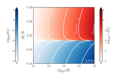
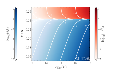
Figure 1: Dimensionless magnetically modified tidal deformability $\delta\Lambda$ shown as a function of magnetic field strength and compactness $M/R$ of the star. The left panel refers to the neutron-star EOS APR, while the right one to the EOS MIT2cfl, and is therefore representative of quark stars. Two different colours are used account for the different signs of $\delta\Lambda$ and indicate that while a magnetic field increases the tidal deformation for weak gravitational fields, it opposes it in stronger gravity.

The results of the numerical integration of the magnetically modified dimensionless tidal deformability (or simply “dimensionless magnetic tidal deformability”) $\delta\Lambda$ are shown in Fig. 1 as a function of magnetic-field strength at the stellar pole for neutron stars with the APR EOS (left panel) and for quark stars with the MIT2cfl EOS (right panel). Note that because the dimensionless magnetic tidal deformability can change sign for sufficiently large compactnesses, we report, respectively in blue and red, the positive and negative values of $\delta\Lambda$. Note also that the sign change takes place at essentially a constant value of the stellar compactness, i.e., at $M/R\simeq 0.205$. The existence of such a zero can be easily deduced from the functional form of $\delta k_{2}$ as given in Eq. (62): since the constant $c_{2}$ is proportional to the stellar radius and because the ratio $d^{e}_{1}/c^{e}_{2}$ become negative above a certain compactness, expression (62) highlights that the magnetic tidal deformability will be zero for a given compactness. From a more physical point of view, the behaviour shown in Fig. 1 highlights the fact that for weak gravitational fields (i.e., for small $M/R$), the presence of a magnetic field simply enhances the tidal deformability as the quadrupolar deformation introduced by the magnetic field adds positively to that introduced by the tidal field. However, for strong gravitational fields (i.e., for large $M/R$), the opposite is true and the magnetic field prevents – via the additional magnetic pressure and magnetic tension – a quadrupolar deformation.

This behaviour can also be found in quark stars (right panel of Fig. 1), although the change in sign in $\delta\Lambda$ takes place at much larger masses and compactnesses (i.e., $M\simeq 2.03\ M_{\odot},\ M/R\simeq 0.245$ for the MIT2cfl EOS). Furthermore, in quark stars, $\delta\Lambda$ decreases monotonically with increasing compactness. These different behaviours at low compactnesses is most likely due to the different behaviour of the outer layers of the two stellar types. In general, in fact, the crust of neutron star follows an EOS that is very different from that of the core. On the other hand, by lacking a crust, quark stars have a behaviour that does not change with compactness and hence yields a magnetic tidal deformability that is mostly positive.

Note also that since $a_{1},\mu\propto B$ [cf. Eqs. (21) and (27)], it follows that $m_{0}^{\rm B},P_{0}\propto B^{2}$ [cf. Eqs. (17)–(18)], so both the constants $c_{2}$ and $d_{1}^{e}$ are proportional to $B^{2}$ [cf. Eqs. (54) and (56)]. As a result, the behaviour of $\delta\Lambda$ as a function of the magnetic field reported in Fig. 1 is actually a linear one. Overall, for the APR EOS, the maximum value of the magnetic tidal deformability is $\delta\Lambda=53.9$ and is reached at $M/R=0.133$ for a magnetic field of $B=10^{16}\,{\rm G}$; this is roughly $4\%$ of $\Lambda^{\rm T}$; on the other hand, for the MIT2cfl the value is $\delta\Lambda=288.7$ at $M/R=0.133$ for a magnetic field of $B=10^{16}\,{\rm G}$; this is roughly $6\%$ of $\Lambda^{\rm T}$.

Figure 2 provides a different view of the dependence of magnetic tidal deformability by reporting in the left panel $\delta\Lambda$ as a function of the stellar compactness for various EOSs relative to neutron stars (bottom part) and quark stars (top part), with a filled circle marking the reference value of the compactness of a star with $M=1.4\,M_{\odot}$. The data in the figure refers to a reference magnetic field of $B=10^{15}\,{\rm G}$ but, obviously, larger/smaller values would be obtained for $\delta\Lambda$ when considering larger/smaller values of $B$. Note the very different behaviour between the two types of stars, with $\delta\Lambda$ having a local maximum in the case of neutron stars, while decreasing monotonically for increasing compactness in the case of quark stars. More importantly, note that the modification of the tidal deformability for quark stars is significantly larger, being even 20 times larger than that of neutron stars. Overall, the different magnitude and dependence on the stellar compactness could provide an important signature to distinguish between the two classes of stars.

Shown instead in the right panel of Fig. 2 is the relative change of the tidal deformability, $\delta\Lambda/\Lambda^{\rm T}$, highlighting that the magnetically induced corrections to the tidal deformability are normally only a small fraction of the ordinary tidal deformation, i.e., $\lesssim 10^{-3}$ for magnetic field as large as $\sim 10^{15}\,{\rm G}$ and $\lesssim 10^{-9}$ for more realistic magnetic fields of $\sim 10^{12}\,{\rm G}$.

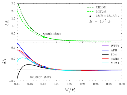
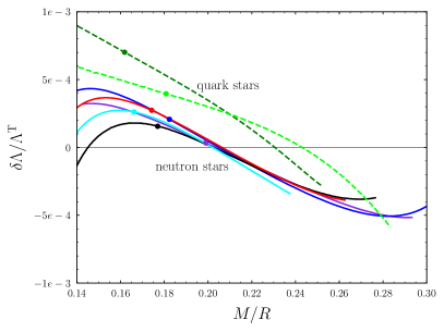
Figure 2: Left panel: Dimensionless magnetic tidal deformability $\delta\Lambda$ shown as a function of the stellar compactness and for a fixed magnetic field of $B=10^{15}\,{\rm G}$. The top part refers to quark-star EOSs, while the bottom one to representative neutron-star EOSs. Marked with dots are the positions of stars with $M=1.4\ M_{\odot}$. Right panel: Relative weight of the dimensionless magnetic tidal deformability $\delta\Lambda$ when compared with the tidal deformability $\Lambda^{\rm T}$. Different lines refer to different EOSs.

III.2 Impact of the phase evolution in binary systems

In order to study the impact that the magnetic tidal deformability has on the evolution of the GW signal from merging binaries, we have computed the GW-phase evolution of representative binaries for the various EOSs considered here and contrasted the situations in which the magnetic field is either zero or not. We recall that GW waveforms of inspiralling binaries are normally calibrated by fitting the numerical-relativity results of the late-inspiral and merger phases, so they can extend the waveforms essentially up to merger (see Hinderer et al. (2018); Dietrich et al. (2020) for two recent reviews). Generally, the most common semi-analytical models are the phenomenological (“Phenom”) models – which combine in a phenomenological manner and at different frequencies the PN evolution with the one from numerical simulations Ajith et al. (2008); Hannam et al. (2014); Khan et al. (2016) – and the effective-one-body (“EOB”) models – which convert the binary inspiral two-body problem to a one-body problem of describing a test particle moving in a deformed black-hole spacetime Buonanno and Damour (1999). Two different and independent EOB models are being developed in the literature, i.e., the SEOBNRv4 Bohé et al. (2017); Cotesta et al. (2018) and the TEOBResumS models, Nagar et al. (2018, 2019), and their differences are discussed in Ref. Rettegno et al. (2019). There are two different ways that the tidal contribution to the waveform are take into account: It can be incorporated directly into EOB formalism in the case of TEOBResumS and SEOBNRv4 models. Alternatively, it can also appear as an additional correction to the tide-free expression for the GW-phase evolution in the case of the SEOBNRv4 and Phenom models.

For convenience, we have here employed the tidal model NRTidal Dietrich et al. (2019), to calculate the contribution of tidal deformability to the GW-phase evolution, while the IMRPhenomD model Khan et al. (2016) is used to handle the black-hole binary part of the inspiral. In practice, we have employed the publicly available PyCBC software Nitz et al. (2020) to generate the waveforms produced by an equal-mass binary of compact stars with single mass $M=1.4\ M_{\odot}$, magnetic fields of various strength, starting from an initial frequency of $60\,{\rm Hz}$ and up to the merger time. In this way, it is possible to define the GW phase differences between the tidal effects with and without magnetic field as

$$\Delta\phi(t):=\left.\phi(t)\right|_{B\neq 0}-\left.\phi(t)\right|_{B=0}\,.$$ (69)

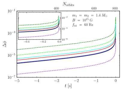
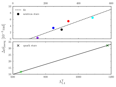
Figure 3: Left panel: Evolution of the GW phase differences $\Delta\phi$ relative to binaries with zero magnetic field or with $B=10^{15}\,{\rm G}$. Different lines refer to different EOSs, but are all relative to a binary with masses $m_{1}=m_{2}=1.4\,M_{\odot}$, that enters the detector at an initial frequency of $60\,{\rm Hz}$. The inset shows a magnification near the merger. Right panel: Final phase difference at the merger $\Delta\phi|_{\rm merg}$ shown as a function of the tidal deformability of a star with $M=1.4\,M_{\odot}$. The top part refers neutron stars, while the bottom part to quark stars; the colour code used is the same as in the left panel and hints to a linear behavior for neutron stars.

Figure 3 reports in its left panel the evolution of the phase difference for a reference magnetic field $B=10^{15}\,{\rm G}$ and for different EOSs relative to either neutron stars (solid lines) or quark stars (dashed lines), using the same colour convention as in Fig. 2. Note that the phase differences are computed up to the merger frequency, which was shown to follow a universal relation with the tidal deformability $\Lambda^{\rm T}$ Read et al. (2013); Bernuzzi et al. (2015); Takami et al. (2015); Rezzolla and Takami (2016) in the case of hadronic stars. It is presently unclear if such universal relations hold also for quark stars and, if so, whether they have the same functional behaviour. Since the PyCBC software does not discriminate between the two classes of compact stars, we have used the same universal relations to compute the GW signal of quark stars up to the presumed merger frequency.

Not surprisingly, the growth of the phase difference reported in the left panel of Fig. 3 is very small apart from the final fractions of a second preceding the merger (see inset). This is obviously due to the fact that tidal effects become important only when the two compact stars have reached a very small separation. Note also that magnetised quark stars yield much large dephasing, which can be one or even two orders of magnitude larger than the corresponding one obtained in the case of neutron stars. Also in this case, however, such changes are comparatively large because of the large reference magnetic fields, so that the values reported serve mostly as upper limits.

Shown instead in the right panel of Fig. 3 is the final GW-phase difference at merger for a reference magnetic field of $10^{15}\,{\rm G}$, different EOSs, and when shown as a function of the tidal deformability of a $1.4\,M_{\odot}$ star $\Lambda^{\rm T}_{1.4}$. The upper part of the panel refers to neutron stars (filled circles), while the lower part to quark stars (crosses). Furthermore, while $\Delta\phi_{\rm merg}=\mathcal{O}\left(10^{-3}\right)\,{\rm rad}$ for such a large magnetic field, much smaller phase differences are measured for more realistic magnetic fields, with an overall trend $\Delta\phi_{\rm merg}\sim B^{2}$. As a result, exploiting the overall behaviour shown by the neutron-star EOSs considered here, it is possible to recognise a linear dependence of the maximum phase difference of the type $\Delta\phi_{\rm merg}=a+b\,\Lambda^{\rm T}_{1.4}$, with $a=-1.873\,(B/10^{15}\,{\rm G})^{2}$ and $b=0.018\,(B/10^{15}\,{\rm G})^{2}$.

Figure 4 shows the phase difference as function of time and of the magnetic-field strength in the range from $10^{14}\,{\rm G}$ to $10^{16}\,{\rm G}$. The left and right panels refer to the APR and to the MIT2cfl EOSs, respectively. Also in this case, we stress that these magnetic fields are considered here not because they are particularly realistic, but because they serve to set stringent upper limits on the impact that magnetic fields may have on the GW-phase evolution. In particular, assuming the extreme case of a magnetic field $B=10^{16}\,{\rm G}$, the final phase difference at merger is $\Delta\phi_{\rm merg}\lesssim 0.65\,{\rm rad}$ for the neutron-star EOSs considered here, and $\Delta\phi_{\rm merg}\lesssim 3.2\,{\rm rad}$ for quark-star EOSs. All of this information, together with the representative values of the magnetic tidal deformabilities, are summarised in Table 1.

Table 1: Summary of the most important quantities computed here for the various EOSs considered. Reported in the various columns are: the dimensionless tidal deformability $\Lambda^{\rm T}$, the dimensionless magnetic deformability $\delta\Lambda$, its relative weight with respect to the dimensionless tidal deformability $\delta\Lambda/\Lambda^{\rm T}$, the final phase differences at merger $\Delta\phi_{\rm merg}$. All quantities are computed for a reference magnetic field of $B=10^{15}\,{\rm G}$ and a stellar mass of $1.4\,M_{\odot}$, whose corresponding stellar radius $R_{1.4}$ is reported on the last column.

	$\Lambda^{\rm T}_{1.4}$	$\left(\delta\Lambda\right)_{1.4}$	$\left(\delta\Lambda/\Lambda^{\rm T}\right)_{1.4}$	$\Delta\phi|_{\rm merg}$	$R_{1.4}$
		$[10^{-2}]\ \$	$[10^{-4}]\ \ \ \ \$	$[10^{-3}\,{\rm rad}]$	$[{\rm km}]\$
${\rm WFF1}$	$151$	$0.495$	$0.328$	$0.294$	$10.39$
${\rm APR}$	$247$	$5.109$	$2.067$	$3.350$	$11.34$
${\rm SLy4}$	$298$	$4.636$	$1.557$	$2.843$	$11.68$
${\rm qmf18}$	$339$	$9.273$	$2.737$	$5.432$	$11.87$
${\rm MPA1}$	$486$	$12.693$	$2.609$	$6.505$	$12.44$
${\rm CIDDM}$	$1177$	$82.557$	$7.014$	$32.168$	$12.77$
${\rm MIT2cfl}$	$650$	$25.653$	$3.950$	$11.813$	$11.43$

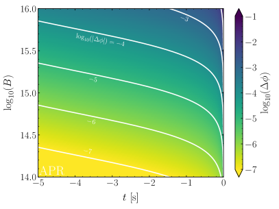
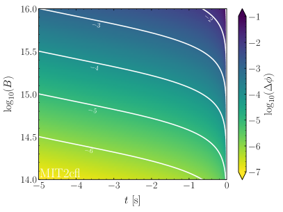
Figure 4: Evolution of the GW phase differences $\Delta\phi$ shown as a function of different magnetic-field strengths. Also in this case, the data refers to a representative binary with masses $m_{1}=m_{2}=1.4\,M_{\odot}$, that enters the detector at an initial frequency of $60\,{\rm Hz}$. The left panel refers to the neutron-star EOS APR, while the right one to the EOS MIT2cfl, and is therefore representative of quark stars.

III.3 Comparison with other high-order corrections

In addition to the corrections introduced by the presence of a magnetic field, there are also some other high-order corrections to the tidal deformability that can have an impact on the GW emission. In particular, as anticipated in Sec. I, given an odd-parity external quadrupolar tidal field, $\mathcal{S}_{ij}$, there will be an odd-parity response of the star in terms of the stellar mass-current quadrupole moment. This tidal deformability can be obtained by looking at the $g_{tj}$ component of metric at a large distance $r$ from the star Hinderer et al. (2018)

$$g_{tj} = -\frac{8}{r^{3}}\epsilon_{ijp}\mathcal{S}^{p}_{\ k}n^{<ki>}+\mathcal{O}\left(r^{-4}\right)+\frac{2}{3}\epsilon_{jpq}\mathcal{B}^{q}_{\ k}\,r^{2}n^{<pk>}+\mathcal{O}\left(r^{3}\right)\,,$$ (70)

where $\mathcal{S}_{ij}$ is the stellar mass-current quadrupole moment, $\mathcal{B}_{ij}$ is the odd-parity induced quadrupolar tidal field, and $n^{<ki>}:=n^{k}n^{i}-\delta^{ki}$ is the symmetric and trace-free projection tensor.

As discussed in Sec. I, the odd-parity quadrupolar tidal deformability $\sigma_{2}$ can be defined as the ratio [cf. Eq. (2)]

$$\sigma_{2}:=\frac{\mathcal{S}_{ij}}{\mathcal{B}_{ij}}\,,$$ (71)

from which it is possible to build a dimensionless odd-parity tidal deformability $j_{2}$

$$j_{2}:=\frac{48}{R^{5}}\sigma_{2}=\frac{48}{R^{5}}\frac{\mathcal{S}_{ij}}{\mathcal{B}_{ij}}\,,$$ (72)

which appears as a correction to the GW-phase evolution at 6PN order, in contrast with the even-parity tidal deformability, which appears at 5PN order (see Refs. Yagi (2014); Banihashemi and Vines (2020); Jiménez Forteza et al. (2018) for more details).

We note that even in the absence of a magnetic field, other high-order corrections to the GW-phase evolution emerge if the tidally deformed star is rotating. In this case, in fact, couplings appear between multipole moments of different parity. For instance, the odd-parity octupole tidal field could produce an even-parity mass quadrupole moment, and the even-parity octupole tidal field could induce an odd-parity mass-current quadrupole moment Pani et al. (2015a, b). The corresponding tidal deformabilities are denoted as $\lambda_{23}$ and $\sigma_{23}$ and contribute to the GW-phase evolution starting from the 6.5PN order, which is also the order at which the corrections from the coupling of the stellar spin with the even-parity tidal deformability also emerge. However, because the inclusion of these rotational corrections in the Lagrangian formulation of the binary dynamics remains conceptually unclear Abdelsalhin et al. (2018); Jiménez Forteza et al. (2018), they will be ignored here, as done in Jiménez Forteza et al. (2018) (see also Poisson (2020a) for an additional source of concern on the magnitude of these corrections).

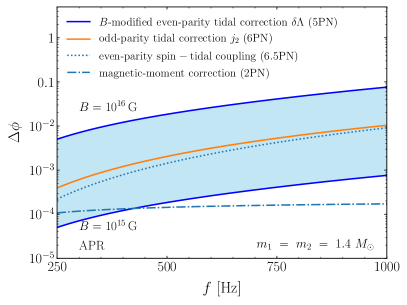
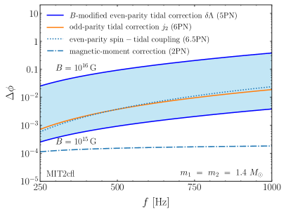
Figure 5: Evolution of the GW phase differences $\Delta\phi$ during the early inspiral (i.e., for frequencies up to $1\,{\rm kHz}$). Shown as a comparison are the other the high-order non-magnetic corrections, i.e., the odd-parity tidal correction $j_{2}$, the even-parity spin-tidal coupling, and the magnetic-moment correction. The blue-shaded region refers to magnetic-field strengths between $10^{15}\,{\rm G}$ and $10^{16}\,{\rm G}$. All the data refers to a representative binary with masses $m_{1}=m_{2}=1.4\,M_{\odot}$, with the left panel relative the APR EOS and the right one to the MIT2cfl EOS.

All of the high-order corrections to the GW-phase evolution discussed above are shown in Fig. 5 as a function of the GW frequency during the inspiral of an equal-mass binary with single mass $M=1.4\ M_{\odot}$ and the APR EOS (left panel) or the MIT2cfl EOS (right panel). Note that because the post-Newtonian approximation breaks down near the merger, the phase difference is considered only up to a frequency of $1000\,{\rm Hz}$. Shown in particular with a blue-shaded region is the contribution of the magnetic tidal deformability with a magnetic field strength from $10^{15}\,{\rm G}$ to $10^{16}\,{\rm G}$. Overall, Fig. 5 shows that the contribution of odd-parity tidal deformability and the even-parity spin-tidal corrections for a dimensionless spin of $\chi=0.05$ (low-spin prior of GW170817) are quite similar in size and frequency dependence. Both of them are larger than the even-parity magnetic tidal deformability for $B=10^{15}\,{\rm G}$, but weaker than that for $B=10^{16}\,{\rm G}$.

Finally, we note that when the two stars are magnetised, the GW-phase evolution during the inspiral is modified not only by pure gravitational effects (i.e., by the tidal deformation of the two stars), but also by the loss of orbital energy to electromagnetic waves. The two stars, in fact, can be assimilated to inspiralling dipoles that will generate electromagnetic waves carrying away energy and angular momentum. The corresponding correction to the binary dynamics appears at 2PN order and was first computed by Ioka and Taniguchi Ioka and Taniguchi (2000). Reported with dot-dashed lines in Fig. 5 is the strength of this correction when calculated self-consistently with our magnetic-field structure and for $B=10^{15}\,{\rm G}$. Clearly, this is the smallest of the high-order contributions – i.e., between two and three orders of magnitude smaller than the magnetically induced corrections to the tidal deformability – and grows only mildly with frequency, i.e., as $f^{1/3}$.

In order to quantify the differences introduced by a magnetic field in the GW waveforms of inspiralling binaries, we have computed the overlap $\mathcal{O}$ between waveforms with or without magnetic field for different EOSs and different detectors. We recall that the overlap is defined as

$$\mathcal{O} := \frac{\langle h_{\delta\Lambda}|h_{0}\rangle}{\sqrt{\langle h_{\delta\Lambda}|h_{\delta\Lambda\rangle}\langle h_{0}|h_{0}\rangle}}\,,$$ (73)

where the scalar product $\langle h_{\delta\Lambda}|h_{0}\rangle$ is given by

$$\langle h_{\delta\Lambda}|h_{0}\rangle := \int_{0}^{\infty}\frac{\tilde{h}_{\delta\Lambda}(f)\tilde{h}_{0}^{\ast}(f)}{S_{h}(f)}df\,.$$ (74)

Here, $h_{\delta\Lambda}$ and $h_{0}$ represent the GW waveforms in the time domain with and without $B$-modified tidal corrections, while $\tilde{h}_{\delta\Lambda}$ and $\tilde{h}_{0}$ are the corresponding Fourier transforms. Furthermore, since it is important to relate the overlap with the actual sensitivity of a given detector, the quantity $S_{h}(f)$ appearing in (74) is the noise power spectral density of the detector under consideration, which in our analysis has been considered for Advanced LIGO and ET.

In this way, we have found that across the various EOSs considered and for a reference magnetic field $B=10^{15}\,{\rm G}$, the mismatch, i.e., $\mathcal{M}:=1-\mathcal{O}$, is always extremely small and of the order $\mathcal{M}\sim\ 10^{-9}$. These values are also much smaller than the experimental limit for advanced LIGO, namely, $\mathcal{O}\simeq 0.005$ Lindblom et al. (2008); Giacomazzo et al. (2009); an exception to this behaviour is offered by the quark-EOS ${\rm CIDDM}$, which is the one leading to the largest phase difference. In this case, and for an ultra-strong magnetic field $B=10^{16}\,{\rm G}$, we find the mismatch to be $\mathcal{M}=0.003$, and thus slightly smaller than the limit for LIGO.

Unfortunately, the use of a third-generation detector such as ET does not help to increase the mismatch. This is because although the differences in the waveforms obviously increase with a more sensitive detector that will record a larger number of GW cycles, the total length of the waveforms will also increase and so the normalisation in the denominator of Eq. (73). Fortunately, however, third-generation detectors will also be able to have a finer determination of the tidal deformability, i.e., with a smaller experimental uncertainty. This was considered in Ref. Jiménez Forteza et al. (2018), where the posterior distributions of the tidal deformability $\tilde{\Lambda}$ were computed when considering the odd-parity tidal correction $j_{2}$. In that case, it was shown that because of the high sensitivity of ET, the posterior distributions of $\tilde{\Lambda}$ – estimated when $j_{2}$ is computed for either an irrotational or static fluid – showed a significant difference (see Fig. 6 in Jiménez Forteza et al. (2018)). Since we have shown in Fig. 5 that the odd-parity tidal correction $j_{2}$ is actually smaller than the magnetic tidal deformability $\delta\Lambda$ when an extreme magnetic field of $B=10^{16}\,{\rm G}$ is considered, it is possible that third-generation detectors would be able measure the contributions to the phase evolution coming from the presence of ultra-strong magnetic fields.

All things considered, we conclude that magnetically induced corrections to the tidal deformability will determine changes in the GW-phase evolution that are unlikely to be detected for realistic values of the magnetic field (i.e., $B\sim 10^{10}-10^{12}\,{\rm G}$), but that are likely to produce a sizeable contribution should unrealistically large magnetic fields (i.e., $B\sim 10^{16}\,{\rm G}$) be present in the two stars prior to merger.

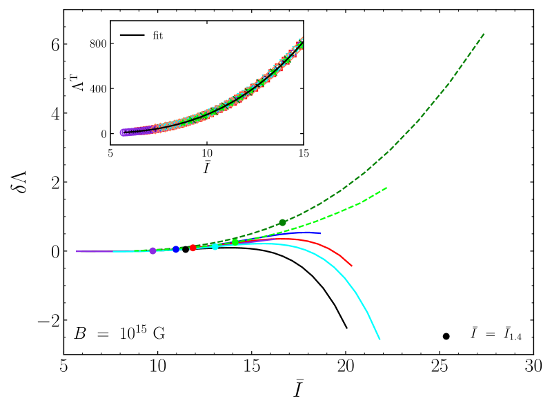
Figure 6: Broken universal relation between the magnetic tidal deformability and the dimensionless moment of inertia $\bar{I}:=I/M^{3}$ for different EOSs and for a magnetic field of $B=10^{15}\,{\rm G}$ (different magnetic-field strengths will only rescale the vertical axis but do not change the functional behaviour). The loss of universality between $\delta\Lambda$ and $\bar{I}$ does not impact significantly the overall universality between $\Lambda$ and $\bar{I}$ (see inset).

III.4 On the validity of universal relations

The last topic we will discuss briefly here is the issue of the validity of the quasi-universal relations that have been shown to exist between the moment of inertia, the Love number, and the mass quadrupole of nonrotating compact stars Yagi and Yunes (2013). While these relations have been demonstrated to hold under a very broad set of conditions (see Yagi and Yunes (2017); Doneva and Pappas (2018) for some recent reviews), they have also been shown to be lost in the case of strong magnetic fields Haskell et al. (2014), or to be modified during the inspiral Maselli et al. (2013). Since such strong magnetic fields are often invoked in our analysis of the tidal deformability, it is reasonable to consider under what conditions the universal relations between the magnetic tidal deformability $\delta\Lambda$ and the moment of inertia $I$ break-down when considering the poloidal magnetic-field configurations explored here.

We note that a somewhat similar analysis was carried out in Ref. Haskell et al. (2014), which was however focused on the validity of the universal relation between the moment of inertia $I$ and the stellar quadrupole moment $Q$ when considering a twisted-torus magnetic topology Ciolfi et al. (2009); Ciolfi and Rezzolla (2013). In that work, it was found that for simple magnetic-field configurations that are purely poloidal or purely toroidal, the relation between the stellar quadrupole moment $Q$ and the moment of inertia $I$ is nearly universal. However, different magnetic field geometries lead to different $I$–$Q$ relations, and, in the case of a twisted-torus configuration, the relation depends significantly on the EOS, losing its universality. In particular, universality was found to be lost for stars with long spin periods, i.e., $P\gtrsim 10\,{\rm s}$, and strong magnetic fields, i.e., $B\gtrsim 10^{12}\,{\rm G}$.

The results of the analysis for the $I$-$\Lambda$ universal relation is summarised in Fig. 6, which reports in the main panel $\delta\Lambda$ as a function of the dimensionless moment of inertia $\bar{I}:=I/M^{3}$ for different EOSs and for a magnetic field of $B=10^{15}\,{\rm G}$ (different magnetic-field strengths will only change the vertical scale, but not the functional behaviour); marked with filled circles are the values for $1.4\,M_{\odot}$ stars. What can be easily appreciated from the main panel in Fig. 6 is that no universal relation can be found between $\delta\Lambda$ and $\bar{I}$ and that the curves relative to different EOSs deviate form a universal behaviour for $\bar{I}\gtrsim 10$. Furthermore, quark stars and neutron stars show a distinctively different behaviour, with $\delta\Lambda$ increasing monotonically with $\bar{I}$, while decreasing for neutron stars. Indeed, we have already encountered a similar behaviour in Fig. 2 and this does not come as a surprise since $\bar{I}\sim(R/M)^{2}$. As a final remark, we note that the loss of universality between $\delta\Lambda$ and $\bar{I}$ does not impact significantly the overall universality between $\Lambda$ and $\bar{I}$, which is preserved by the fact that $\delta\Lambda\ll\Lambda^{\rm T}$, and that $\Lambda^{\rm T}$ still correlates universally with $\bar{I}$ for $\bar{I}\lesssim 15$, as shown in the inset in Fig. 6.

IV Conclusions

The evolution of the GW phase produced by inspiralling binaries of compact stars is subject to corrections coming from the nonzero deformability of the two stars. In turn, because the tidal deformability is directly related to the properties of the EOS of nuclear matter, the measurement of these corrections promises to be an important tool to read-off the EOS from the GW signal. Extensive work has been carried out over the last decade to quantify in an even more accurate manner the size of these corrections when taking into account a number low- and high-order corrections to the tidal deformability coming, for instance, by mass-current multipoles or by the presence of an intrinsic spin in the star. This bulk of work has reached a considerable level of sophistication and a rather comprehensive view of this problem is now available in the literature.

We have here considered an aspect of this research that has not been explored so far, namely, the high-order corrections to the tidal deformability that are introduced by the presence of an intrinsic magnetic field in the stars. These corrections should not be confused with the “gravitomagnetic” (or odd-parity) corrections to the tidal deformability, namely, with the “even-parity” quadrupolar tidal deformability, which starts to impact the phase of the GW signal at 5PN.

At the order considered here, the magnetic field induces correction only to the even-parity quadrupole moment and we assume that it does not lead to coupling of different multipole moments. However, because these represent a correction to the standard unmagnetised, nonspinning tidal deformability, they impose an analysis that includes second-order perturbations. Proceeding in this way, we were able to compute the magnetic-field induced changes to the tidal deformability and to assess their impact on the evolution of the GW phase for different strengths of the magnetic field and for different EOSs, including those that describe quark stars. Overall, we find that magnetically induced corrections to the tidal deformability will produce changes in the GW-phase evolution that are unlikely to be detected if the magnetic field has the strength expected from astrophysical considerations, i.e., $B\sim 10^{10}-10^{12}\,{\rm G}$. At the same time, if the magnetic field present in the two stars prior to merger is unrealistically large, i.e., $B\sim 10^{16}\,{\rm G}$, these corrections are expected to produce a sizeable contribution to the GW-phase evolution measured by third-generation detectors such as ET and CE. In this unlikely event, and if the neglected higher-order terms will remain negligible also for very high magnetic fields, the induced phase differences would represent a very useful tool to study and measure the properties of the magnetic fields in the merging stars, thus providing information that is otherwise hard to quantify.

Appendix A Details on the derivation

In what follows we provide details on the derivation of the perturbative equations presented in the main text and that were omitted from compactness. We start by recalling that the the nonvanishing components of the perturbed Einstein tensor are $\delta G_{\ 0}^{0}$, $\delta G_{\ i}^{i}$ and $\delta G_{\ 1}^{2}$. In particular, the Einstein equation $\delta G_{\ 2}^{2}-\delta G_{\ 3}^{3}=0$ can be used to obtain a relation between $\delta H_{0}$ and $\delta H_{2}$ as

$$\delta H_{0}+\delta H_{2}=A_{23}\,,$$ (75)

where $A_{23}$ is an additional term resulting from the first-order perturbation

$$A_{23}:= -\frac{4}{7}\biggl{[}H_{0}h_{2}^{\rm B}-\frac{H_{0}m_{2}^{\rm B}e^{\lambda}}{r}\biggr{]}+\biggl{[}2h_{0}^{\rm B}H_{0}-\frac{2H_{0}m_{0}^{\rm B}e^{\lambda}}{r}\biggr{]}$$

$$-\frac{4}{21}\biggl{[}3Kh_{2}^{\rm B}+2Ke^{-\lambda}(a_{1}^{\prime})^{2}+3H_{0}h_{2}^{\rm B}+\frac{3Km_{2}^{\rm B}e^{\lambda}}{r}-\frac{3H_{0}m_{2}^{\rm B}e^{\lambda}}{r}\biggr{]}$$

$$+\frac{6}{7}\biggl{[}H_{0}h_{2}^{\rm B}+\frac{Km_{2}^{\rm B}e^{\lambda}}{r}-\frac{H_{0}m_{2}^{\rm B}e^{\lambda}}{r}+Kh_{2}^{\rm B}\biggr{]}\,.$$ (76)

Similarly, the Einstein equation $\delta G_{\ 1}^{2}=8\pi\delta T_{\ 1}^{2}=0$ can be exploited to relate $\delta H_{0}$ and $\delta K^{\prime}$ as

$$\frac{r^{2}\nu^{\prime}}{4}\biggl{(}\delta H_{0}^{\ell}-\delta H_{2}^{\ell}\biggr{)}+\frac{r^{2}}{2}\biggl{(}\delta K_{\ell}^{\prime}+\delta H_{0}^{l\prime}\biggr{)}-\frac{r}{2}\biggl{(}\delta H_{0}^{\ell}+\delta H_{2}^{\ell}\biggr{)}=B_{12}\,,$$ (77)

where $B_{12}$ is defined as

$$B_{12}:= \frac{2}{7}r^{2}Kk_{2}^{{\rm B}\prime}+\frac{1}{7}\left[\frac{r^{2}\nu^{\prime}}{2}H_{0}h_{2}^{\rm B}+r^{2}H_{0}^{\prime}h_{2}^{\rm B}+r^{2}K^{\prime}k_{2}^{\rm B}-rH_{0}h_{2}^{\rm B}+\frac{r\nu^{\prime}H_{0}m_{2}^{\rm B}e^{\lambda}}{2}\right]$$

$$+\left[\frac{r^{2}\nu^{\prime}}{2}H_{0}h_{0}^{\rm B}+r^{2}H_{0}^{\prime}h_{0}^{\rm B}+\frac{r\nu^{\prime}H_{0}m_{0}^{\rm B}e^{\lambda}}{2}-rH_{0}h_{0}^{\rm B}+H_{0}m_{0}^{\rm B}e^{\lambda}\right]$$

$$-\frac{1}{7}\biggl{[}r^{2}H_{0}k_{2}^{{\rm B}\prime}+\frac{r^{2}\nu^{\prime}H_{0}h_{2}^{\rm B}}{2}-r^{2}K^{\prime}k_{2}^{\rm B}-\frac{r\nu^{\prime}H_{0}m_{2}^{\rm B}e^{\lambda}}{2}\biggr{]}$$

$$+\frac{4}{21}Ka_{1}a_{1}^{\prime}+\frac{3}{7}H_{0}m_{2}^{\rm B}e^{\lambda}\,.$$ (78)

The remaining Einstein equations are

$$\delta G_{\ 0}^{0}-\delta G_{\ 1}^{1}=-8\pi\left(1+\frac{1}{c_{s}^{2}}\right)\,\delta p^{\rm BT}\,,$$ (79)

$$\delta G_{\ 2}^{2}-\delta G_{\ 3}^{3}=16\pi\delta p^{\rm BT}\,,$$ (80)

where $\delta p^{\rm BT}$ is the second-order pressure perturbation. We can further define two functions, $C_{01}$ and $C_{23}$, to simplify Eqs. (79), (80) as

$$C_{01}:= \frac{2}{7}\biggl{[}K\biggl{(}\lambda^{\prime}k_{2}^{{\rm B}\prime}+\nu^{\prime}k_{2}^{{\rm B}\prime}-2k_{2}^{{\rm B}\prime\prime}\biggr{)}e^{-\lambda}-H_{0}\biggl{(}\lambda^{\prime}k_{2}^{{\rm B}\prime}+\nu^{\prime}k_{2}^{{\rm B}\prime}-2k_{2}^{{\rm B}\prime\prime}\biggr{)}e^{-\lambda}-K^{\prime}\biggl{(}h_{2}^{{\rm B}\prime}+2k_{2}^{{\rm B}\prime}\biggr{)}e^{-\lambda}$$

$$+\biggl{(}K^{\prime}\lambda^{\prime}+K^{\prime}\nu^{\prime}-2K^{\prime\prime}\biggr{)}k_{2}^{\rm B}e^{-\lambda}-4\biggl{(}K-H_{0}\biggr{)}\frac{k_{2}^{{\rm B}\prime}e^{-\lambda}}{r}+\frac{2H_{0}^{\prime}h_{2}^{\rm B}e^{-\lambda}}{r}-\frac{K^{\prime}m_{2}^{{\rm B}\prime}}{r}-\frac{6Kh_{2}^{\rm B}}{r^{2}}$$

$$-\frac{4K^{\prime}k_{2}^{\rm B}e^{-\lambda}}{r}+\biggl{(}\nu^{\prime}K^{\prime}-2K^{\prime\prime}\biggr{)}\frac{m_{2}^{\rm B}}{r}-\frac{6H_{0}h_{2}^{\rm B}}{r^{2}}-\frac{12H_{0}k_{2}^{\rm B}}{r^{2}}+\frac{4H_{0}}{r^{2}}\biggl{(}\nu^{\prime}m_{2}^{\rm B}-m_{2}^{{\rm B}\prime}\biggr{)}$$

$$-\biggl{(}3K^{\prime}+2H_{0}^{\prime}\biggr{)}\frac{m_{2}^{\rm B}}{r^{2}}-\frac{6H_{0}h_{2}^{\rm B}}{r^{2}}+\frac{6Km_{2}^{\rm B}e^{\lambda}}{r^{3}}+\frac{H_{0}m_{2}^{\rm B}e^{\lambda}}{r^{3}}\biggl{(}4e^{-\lambda}-6\biggr{)}-\frac{6H_{0}m_{2}^{\rm B}e^{\lambda}}{r^{3}}\biggr{]}$$

$$+\biggl{[}\frac{2H_{0}^{\prime}h_{0}^{m}e^{-\lambda}}{r}+\biggl{(}\nu^{\prime}K^{\prime}-2K^{\prime\prime}\biggr{)}\frac{m_{0}^{\rm B}}{r}-\frac{K^{\prime}m_{0}^{{\rm B}\prime}}{r}-K^{\prime}h_{0}^{{\rm B}\prime}e^{-\lambda}-\frac{6H_{0}h_{0}^{\rm B}}{r^{2}}-\biggl{(}3K^{\prime}+2H_{0}^{\prime}\biggr{)}\frac{m_{0}^{\rm B}}{r^{2}}$$

$$+\frac{4H_{0}}{r^{2}}\biggl{(}\nu^{\prime}m_{0}^{\rm B}-m_{0}^{{\rm B}\prime}\biggr{)}+\frac{H_{0}m_{0}^{\rm B}e^{\lambda}}{r^{3}}\biggl{(}4e^{-\lambda}-6\biggr{)}\biggr{]}+\frac{6}{7}\biggl{[}\frac{H_{0}h_{2}^{\rm B}}{r^{2}}+\frac{H_{0}m_{2}^{\rm B}e^{\lambda}}{r^{3}}\biggr{]}+\frac{88}{21}\frac{H_{0}a_{1}^{2}}{r^{4}}\,,$$ (81)

$$C_{23}:= \frac{2}{7}\biggl{[}K\biggl{(}\lambda^{\prime}k_{2}^{{\rm B}\prime}-\nu^{\prime}k_{2}^{{\rm B}\prime}-2k_{2}^{{\rm B}\prime\prime}\biggr{)}e^{-\lambda}-H_{0}\biggl{(}\lambda^{\prime}k_{2}^{{\rm B}\prime}-\nu^{\prime}k_{2}^{{\rm B}\prime}-2k_{2}^{{\rm B}\prime\prime}\biggr{)}e^{-\lambda}+\biggl{(}\lambda^{\prime}H_{0}^{\prime}-2\nu^{\prime}H_{0}^{\prime}-2H_{0}^{\prime\prime}\biggr{)}e^{-\lambda}h_{2}^{\rm B}$$

$$-\frac{64\pi pH_{0}m_{2}^{\rm B}e^{\lambda}}{r}+\biggl{(}\lambda^{\prime}K^{\prime}-\nu^{\prime}K^{\prime}-2K^{\prime\prime}\biggr{)}k_{2}^{\rm B}e^{-\lambda}+\biggl{(}K^{\prime}-H_{0}^{\prime}\biggr{)}\biggl{(}h_{2}^{{\rm B}\prime}-2k_{2}^{{\rm B}\prime}\biggr{)}e^{-\lambda}$$

$$-\frac{4Kk_{2}^{{\rm B}\prime}e^{-\lambda}}{r}+\frac{4H_{0}k_{2}^{{\rm B}\prime}e^{-\lambda}}{r}-\frac{2\nu^{\prime}}{r}H_{0}\biggl{(}\lambda^{\prime}m_{2}^{\rm B}+m_{2}^{{\rm B}\prime}\biggr{)}-\frac{2H_{0}^{\prime}h_{2}^{\rm B}e^{-\lambda}}{r}-\frac{4K^{\prime}k_{2}^{\rm B}e^{-\lambda}}{r}$$

$$-\biggl{(}K^{\prime}\nu^{\prime}+2K^{\prime\prime}+4H_{0}^{\prime}\nu^{\prime}+2H_{0}^{\prime\prime}\biggr{)}\frac{m_{2}^{\rm B}}{r}-\biggl{(}K^{\prime}+H_{0}^{\prime}\biggr{)}\frac{m_{2}^{{\rm B}\prime}}{r}+\frac{6Kh_{2}^{\rm B}}{r^{2}}+\frac{6H_{0}h_{2}^{\rm B}}{r^{2}}$$

$$-\frac{2H_{0}}{r^{2}}\biggl{(}2\lambda^{\prime}m_{2}^{\rm B}-\nu^{\prime}m_{2}^{\rm B}+2m_{2}^{{\rm B}\prime}\biggr{)}-\biggl{(}3K^{\prime}+5H_{0}^{\prime}\biggr{)}\frac{m_{2}^{\rm B}}{r^{2}}+\frac{6H_{0}h_{2}^{\rm B}}{r^{2}}$$

$$+\frac{6Km_{2}^{\rm B}e^{\lambda}}{r^{3}}-\frac{6H_{0}m_{2}^{\rm B}e^{\lambda}}{r^{3}}+\frac{4H_{0}m_{2}^{\rm B}}{r^{3}}-\frac{6H_{0}m_{2}^{\rm B}e^{\lambda}}{r^{3}}\biggr{]}$$

$$\biggl{[}-\frac{64\pi pH_{0}m_{0}^{\rm B}e^{\lambda}}{r}+\biggl{(}\lambda^{\prime}H_{0}^{\prime}-2\nu^{\prime}H_{0}^{\prime}-2H_{0}^{\prime\prime}\biggr{)}h_{0}^{\rm B}e^{-\lambda}+\left(K^{\prime}-H_{0}^{\prime}\right)h_{0}^{{\rm B}\prime}e^{-\lambda}-\frac{2H_{0}^{\prime}h_{0}^{\rm B}e^{-\lambda}}{r}$$

$$-\frac{2\nu^{\prime}H_{0}}{r}\biggl{(}\lambda^{\prime}m_{0}^{\rm B}+m_{0}^{{\rm B}\prime}\biggr{)}-\biggl{(}\nu^{\prime}K^{\prime}+2K^{\prime\prime}+4\nu^{\prime}H_{0}^{\prime}+2H_{0}^{\prime\prime}\biggr{)}\frac{m_{0}^{\rm B}}{r}-\biggl{(}K^{\prime}+H_{0}^{\prime}\biggr{)}\frac{m_{0}^{{\rm B}\prime}}{r}$$

$$+\frac{6H_{0}h_{0}^{\rm B}}{r^{2}}-\frac{2H_{0}}{r^{2}}\biggl{(}2\lambda^{\prime}m_{0}^{\rm B}-\nu^{\prime}m_{0}^{\rm B}+2m_{0}^{{\rm B}\prime}\biggr{)}-\biggl{(}3K^{\prime}+5H_{0}^{l\prime}\biggr{)}\frac{m_{0}^{\rm B}}{r^{2}}+\frac{4H_{0}m_{0}^{\rm B}}{r^{3}}-\frac{6H_{0}m_{0}^{\rm B}e^{\lambda}}{r^{3}}\biggr{]}$$

$$+\frac{6}{7}\biggl{[}\frac{2H_{0}m_{2}^{\rm B}e^{\lambda}}{r^{3}}-\frac{2H_{0}h_{2}^{\rm B}}{r^{2}}\biggr{]}-\frac{88}{21}\frac{Ka_{1}^{2}}{r^{4}}\,.$$ (82)

The final form that Eqs. (79) and (80) then take is

$$C_{01}= -8\pi(1+\frac{1}{c_{s}^{2}})\delta\tilde{P}-\frac{3(\delta H_{0}-\delta H_{2})}{r^{2}}+\frac{e^{-\lambda}}{2}\biggl{(}\lambda^{\prime}\delta K^{\prime}+\nu^{\prime}\delta K^{\prime}-2\delta K^{\prime\prime}\biggr{)}$$

$$-\frac{\delta H_{2}e^{-\lambda}(\lambda^{\prime}+\nu^{\prime})}{r}-\frac{e^{-\lambda}}{r}\biggl{(}2\delta K^{\prime}-\delta H_{0}^{\prime}-\delta H_{2}^{l\prime}\biggr{)}\,,$$ (83)

$$C_{23}= 16\pi\delta\tilde{P}+16\pi p\delta H_{2}+\frac{e^{-\lambda}\delta K^{\prime}(\lambda^{\prime}-\nu^{\prime})}{2}+\frac{e^{-\lambda}}{2}\biggl{(}\lambda^{\prime}\delta H_{0}^{\prime}+\nu^{\prime}\delta H_{2}^{\prime}\biggr{)}$$

$$-e^{-\lambda}\biggl{(}\delta K^{\prime\prime}+\delta H_{0}^{\prime}\nu^{\prime}+\delta H_{0}^{\prime\prime}\biggr{)}-\frac{e^{-\lambda}}{r}\biggl{(}2\delta K^{\prime}+\delta H_{0}^{\prime}-\delta H_{2}^{\prime}\biggr{)}+\frac{3(\delta H_{0}+\delta H_{2})}{r^{2}}\,$$ (84)

where $\delta\tilde{P}$ is defined as

$$\delta\tilde{P} :=\frac{5}{2}\int_{0}^{\pi}\delta p^{\rm BT}P_{2}(\cos\theta)\sin\theta d\theta\,.$$ (85)

Finally, we can substitute in Eq. (A) the expressions for $\delta H_{2}$, $\delta K$, and $\delta\tilde{P}$ given by Eqs. (75)–(77), (A). In this way, we obtain the master equation for $\delta H_{0}$, i.e., Eq. (54), whose source term is explicitly given by

$$S(r) =\biggl{\{}2C_{01}+(1+\frac{1}{c_{s}^{2}})C_{23}-e^{-\lambda}(\lambda^{\prime}+\nu^{\prime})T+2e^{-\lambda}T^{\prime}+\frac{4e^{-\lambda}}{r}T+\frac{6}{r^{2}}A_{23}+\frac{2A_{23}e^{-\lambda}(\lambda^{\prime}+\nu^{\prime})}{r}-\frac{2e^{-\lambda}}{r}A_{23}^{\prime}$$

$$-\left[16\pi pA_{23}+\frac{e^{-\lambda}}{2}A_{23}^{\prime}\nu^{\prime}+\frac{e^{-\lambda}}{r}A_{23}^{\prime}+\frac{3}{r^{2}}A_{23}+\frac{T}{2}e^{-\lambda}(\lambda^{\prime}-\nu^{\prime})-e^{-\lambda}T^{\prime}-\frac{2e^{-\lambda}}{r}T\right](1+\frac{1}{c_{s}^{2}})\biggr{\}}\frac{e^{\lambda}}{2}\,,$$ (86)

where we have defined

$$T :=(r\nu^{\prime}+2)\frac{A_{23}}{2r}+\frac{2B_{12}}{r^{2}}.$$ (87)

The exterior source term is obtained readily after setting to zero the matter terms of Eq. (A) and it is therefore given by

$$S^{e}(z)= \frac{9c_{1}^{e}\mu^{2}}{224M^{4}}(3z^{4}+176z^{3}-180z^{2}-140z-147)\log\left(\frac{z+1}{z-1}\right)^{3}$$

$$+\biggl{[}\frac{3c_{2}^{e}\mu^{2}}{112M^{4}}(3z^{4}+176z^{3}-180z^{2}-140z-147)+\frac{18K^{\rm B}c_{1}^{e}}{7}(4z^{4}+15z^{3}-2z^{2}-15z-2)$$

$$+\frac{3c_{1}^{e}\mu^{2}}{112M^{4}}\frac{72z^{6}+243z^{5}-936z^{4}-1566z^{3}+1216z^{2}+723z-488}{z^{2}-1}\biggr{]}\log\left(\frac{z+1}{z-1}\right)^{2}$$

$$+\biggl{[}\frac{3c_{2}^{e}\mu^{2}}{14M^{4}}\frac{6z^{6}+21z^{5}-34z^{4}-86z^{3}+37z^{2}+9z-37}{z^{2}-1}+\frac{12c_{1}^{e}c_{2}}{M}\frac{-z^{2}+z+2}{z-1}$$

$$+\frac{3c_{1}^{e}\mu^{2}}{56M^{4}}\frac{-144z^{9}-513z^{8}+528z^{7}+2385z^{6}-500z^{5}-2119z^{4}+564z^{3}-621z^{2}-640z+772}{z^{6}-3z^{4}+3z^{2}-1}$$

$$+\frac{12K^{\rm B}c_{2}^{e}}{7}(4z^{4}+15z^{3}-2z^{2}-15z-2)-\frac{24K^{\rm B}c_{1}^{e}}{7}\frac{12z^{5}+45z^{4}-14z^{3}-75z^{2}+6z+12}{z^{2}-1}\biggr{]}\log\left(\frac{z+1}{z-1}\right)$$

$$+\biggl{[}-\frac{3c_{2}^{e}\mu^{2}}{28M^{4}}\frac{24z^{7}+87z^{6}+24z^{5}-224z^{4}-216z^{3}-23z^{2}+132z+228}{z^{4}-2z^{2}+1}+\frac{8c_{2}^{e}c_{2}}{M}\frac{-z^{2}+z+2}{z-1}$$

$$+\frac{3c_{1}^{e}\mu^{2}}{28M^{4}}\frac{72z^{8}+261z^{7}+24z^{6}-846z^{5}-648z^{4}+85z^{3}+456z^{2}+764z-144}{z^{6}-3z^{4}+3z^{2}-1}$$

$$+\frac{8c_{1}^{e}c_{2}}{M}\frac{3z^{3}-3z^{2}-8z+2}{z^{3}-z^{2}-z+1}-\frac{8c_{2}^{e}K^{\rm B}}{7}\frac{12z^{5}+45z^{4}-14z^{3}-75z^{2}+6z+12}{z^{2}-1}$$

$$+\frac{8c_{1}^{e}K^{\rm B}}{7}\frac{36z^{8}+135z^{7}-102z^{6}-450z^{5}+136z^{4}+447z^{3}-110z^{2}-120z+64}{z^{6}-3z^{4}+3z^{2}-1}\biggr{]}.$$ (88)

We conclude by reporting the contribution from surface source term $S_{\rm surf}$ in the matching procedure of Eqs. (64) and (65), namely,

$$S_{\rm surf}(r)= \biggl{(}C_{23}-16\pi pA_{23}-\frac{e^{-\lambda}}{2}A_{23}^{\prime}\nu^{\prime}-\frac{e^{-\lambda}}{r}A_{23}^{\prime}-\frac{3}{r^{2}}A_{23}-\frac{T}{2}e^{-\lambda}(\lambda^{\prime}-\nu^{\prime})+e^{-\lambda}T^{\prime}+\frac{2e^{-\lambda}}{r}T\biggr{)}\biggl{|}_{r=R}\frac{R^{2}}{2M}\,.$$ (89)

References

- Abbott et al. (2017) B. P. Abbott, R. Abbott, T. D. Abbott, F. Acernese, K. Ackley, C. Adams, T. Adams, P. Addesso, R. X. Adhikari, V. B. Adya, and et al. (LIGO Scientific Collaboration and Virgo Collaboration), Phys. Rev. Lett. 119, 161101 (2017), arXiv:1710.05832 [gr-qc] .
- Margalit and Metzger (2017) B. Margalit and B. D. Metzger, Astrophys. J. Lett. 850, L19 (2017), arXiv:1710.05938 [astro-ph.HE] .
- Bauswein et al. (2017) A. Bauswein, O. Just, H.-T. Janka, and N. Stergioulas, Astrophys. J. Lett. 850, L34 (2017), arXiv:1710.06843 [astro-ph.HE] .
- Rezzolla et al. (2018) L. Rezzolla, E. R. Most, and L. R. Weih, Astrophys. J. Lett. 852, L25 (2018), arXiv:1711.00314 [astro-ph.HE] .
- Ruiz et al. (2018) M. Ruiz, S. L. Shapiro, and A. Tsokaros, Phys. Rev. D 97, 021501 (2018), arXiv:1711.00473 [astro-ph.HE] .
- Annala et al. (2018) E. Annala, T. Gorda, A. Kurkela, and A. Vuorinen, Phys. Rev. Lett. 120, 172703 (2018), arXiv:1711.02644 [astro-ph.HE] .
- Radice et al. (2018) D. Radice, A. Perego, F. Zappa, and S. Bernuzzi, Astrophys. J. Lett. 852, L29 (2018), arXiv:1711.03647 [astro-ph.HE] .
- Most et al. (2018) E. R. Most, L. R. Weih, L. Rezzolla, and J. Schaffner-Bielich, Phys. Rev. Lett. 120, 261103 (2018), arXiv:1803.00549 [gr-qc] .
- Tews et al. (2018) I. Tews, J. Carlson, S. Gandolfi, and S. Reddy, Astrophys. J. 860, 149 (2018), arXiv:1801.01923 [nucl-th] .
- De et al. (2018) S. De, D. Finstad, J. M. Lattimer, D. A. Brown, E. Berger, and C. M. Biwer, Physical Review Letters 121, 091102 (2018), arXiv:1804.08583 [astro-ph.HE] .
- Abbott et al. (2018) B. P. Abbott, R. Abbott, T. D. Abbott, F. Acernese, K. Ackley, C. Adams, T. Adams, P. Addesso, R. X. Adhikari, V. B. Adya, and et al. (LIGO Scientific Collaboration and Virgo Collaboration), Physical Review Letters 121, 161101 (2018), arXiv:1805.11581 [gr-qc] .
- Shibata et al. (2019) M. Shibata, E. Zhou, K. Kiuchi, and S. Fujibayashi, Phys. Rev. D 100, 023015 (2019), arXiv:1905.03656 [astro-ph.HE] .
- Koeppel et al. (2019) S. Koeppel, L. Bovard, and L. Rezzolla, Astrophys. J. Lett. 872, L16 (2019), arXiv:1901.09977 [gr-qc] .
- Fattoyev et al. (2018) F. J. Fattoyev, J. Piekarewicz, and C. J. Horowitz, Physical Review Letters 120, 172702 (2018), arXiv:1711.06615 [nucl-th] .
- Paschalidis et al. (2018) V. Paschalidis, K. Yagi, D. Alvarez-Castillo, D. B. Blaschke, and A. Sedrakian, Phys. Rev. D 97, 084038 (2018), arXiv:1712.00451 [astro-ph.HE] .
- Burgio et al. (2018) G. F. Burgio, A. Drago, G. Pagliara, H.-J. Schulze, and J.-B. Wei, Astrophys. J. 860, 139 (2018).
- Montaña et al. (2019) G. Montaña, L. Tolós, M. Hanauske, and L. Rezzolla, Phys. Rev. D 99, 103009 (2019), arXiv:1811.10929 [astro-ph.HE] .
- Gomes et al. (2019a) R. O. Gomes, P. Char, and S. Schramm, Astrophys. J. 877, 139 (2019a), arXiv:1806.04763 [nucl-th] .
- Li et al. (2018) C.-M. Li, Y. Yan, J.-J. Geng, Y.-F. Huang, and H.-S. Zong, Phys. Rev. D 98, 083013 (2018), arXiv:1808.02601 [nucl-th] .
- Li et al. (2020) J. J. Li, A. Sedrakian, and M. Alford, Phys. Rev. D 101, 063022 (2020).
- Zhou et al. (2018) E.-P. Zhou, X. Zhou, and A. Li, Phys. Rev. D 97, 083015 (2018), arXiv:1711.04312 [astro-ph.HE] .
- Most et al. (2019) E. R. Most, L. J. Papenfort, V. Dexheimer, M. Hanauske, S. Schramm, H. Stöcker, and L. Rezzolla, Physical Review Letters 122, 061101 (2019), arXiv:1807.03684 [astro-ph.HE] .
- Bauswein et al. (2019) A. Bauswein, N.-U. F. Bastian, D. B. Blaschke, K. Chatziioannou, J. A. Clark, T. Fischer, and M. Oertel, Physical Review Letters 122, 061102 (2019), arXiv:1809.01116 [astro-ph.HE] .
- Weih et al. (2020) L. R. Weih, M. Hanauske, and L. Rezzolla, Phys. Rev. Lett. 124, 171103 (2020), arXiv:1912.09340 [gr-qc] .
- Pani et al. (2015a) P. Pani, L. Gualtieri, A. Maselli, and V. Ferrari, Phys. Rev. D 92, 024010 (2015a), arXiv:1503.07365 [gr-qc] .
- Harry and Hinderer (2018) I. Harry and T. Hinderer, Classical and Quantum Gravity 35, 145010 (2018), arXiv:1801.09972 [gr-qc] .
- Flanagan and Hinderer (2008) É. É. Flanagan and T. Hinderer, Physical Review D 77, 021502 (2008), arXiv:0709.1915 [astro-ph] .
- Hinderer (2008) T. Hinderer, Astrophys. J. 677, 1216 (2008), arXiv:0711.2420 .
- Hinderer et al. (2010) T. Hinderer, B. D. Lackey, R. N. Lang, and J. S. Read, Phys. Rev. D 81, 123016 (2010), arXiv:0911.3535 [astro-ph.HE] .
- Vines et al. (2011) J. Vines, E. E. Flanagan, and T. Hinderer, Phys. Rev. D 83, 084051 (2011), arXiv:1101.1673 [gr-qc] .
- Damour and Nagar (2009) T. Damour and A. Nagar, Phys. Rev. D 80, 084035 (2009), arXiv:0906.0096 [gr-qc] .
- Binnington and Poisson (2009) T. Binnington and E. Poisson, Phys. Rev. D 80, 084018 (2009), arXiv:0906.1366 [gr-qc] .
- Landry and Poisson (2015) P. Landry and E. Poisson, Phys. Rev. D 91, 104026 (2015), arXiv:1504.06606 [gr-qc] .
- Pani et al. (2018) P. Pani, L. Gualtieri, T. Abdelsalhin, and X. Jiménez-Forteza, Phys. Rev. D 98, 124023 (2018), arXiv:1810.01094 [gr-qc] .
- Yagi (2014) K. Yagi, Phys. Rev. D 89, 043011 (2014), arXiv:1311.0872 [gr-qc] .
- Jiménez Forteza et al. (2018) X. Jiménez Forteza, T. Abdelsalhin, P. Pani, and L. Gualtieri, Phys. Rev. D 98, 124014 (2018), arXiv:1807.08016 [gr-qc] .
- Banihashemi and Vines (2020) B. Banihashemi and J. Vines, Phys. Rev. D 101, 064003 (2020), arXiv:1805.07266 [gr-qc] .
- Abdelsalhin et al. (2018) T. Abdelsalhin, L. Gualtieri, and P. Pani, Phys. Rev. D 98, 104046 (2018), arXiv:1805.01487 [gr-qc] .
- Poisson (2020a) E. Poisson, arXiv e-prints , arXiv:2007.01678 (2020a), arXiv:2007.01678 [gr-qc] .
- Flanagan and Racine (2007) É. É. Flanagan and É. Racine, Physical Review D 75, 044001 (2007), arXiv:gr-qc/0601029 [gr-qc] .
- Steinhoff et al. (2016) J. Steinhoff, T. Hinderer, A. Buonanno, and A. Taracchini, Phys. Rev. D 94, 104028 (2016), arXiv:1608.01907 [gr-qc] .
- Hinderer et al. (2016) T. Hinderer, A. Taracchini, F. Foucart, A. Buonanno, J. Steinhoff, M. Duez, L. E. Kidder, H. P. Pfeiffer, M. A. Scheel, B. Szilagyi, K. Hotokezaka, K. Kyutoku, M. Shibata, and C. W. Carpenter, Phys. Rev. Lett. 116, 181101 (2016), arXiv:1602.00599 [gr-qc] .
- Poisson (2020b) E. Poisson, arXiv e-prints , arXiv:2003.10427 (2020b), arXiv:2003.10427 [gr-qc] .
- Ma et al. (2020) S. Ma, H. Yu, and Y. Chen, arXiv e-prints , arXiv:2003.02373 (2020), arXiv:2003.02373 [gr-qc] .
- Pereira et al. (2020) J. P. Pereira, M. Bejger, N. Andersson, and F. Gittins, Astrophys. J. 895, 28 (2020), arXiv:2003.10781 [gr-qc] .
- Gittins et al. (2020) F. Gittins, N. Andersson, and J. P. Pereira, arXiv e-prints , arXiv:2003.05449 (2020), arXiv:2003.05449 [astro-ph.HE] .
- Giacomazzo et al. (2009) B. Giacomazzo, L. Rezzolla, and L. Baiotti, Mon. Not. R. Astron. Soc. 399, L164 (2009), arXiv:0901.2722 [gr-qc] .
- Punturo et al. (2010) M. Punturo et al., Class. Quantum Grav. 27, 084007 (2010).
- Abbott and et al. (2017) B. P. Abbott and et al., Classical and Quantum Gravity 34, 044001 (2017), arXiv:1607.08697 [astro-ph.IM] .
- Konno et al. (1999) K. Konno, T. Obata, and Y. Kojima, Astron.Astrophys 352, 211 (1999), arXiv:gr-qc/9910038 [gr-qc] .
- Ioka and Sasaki (2004) K. Ioka and M. Sasaki, Astrophys. J. 600, 296 (2004), arXiv:astro-ph/0305352 .
- Colaiuda et al. (2008) A. Colaiuda, V. Ferrari, L. Gualtieri, and J. A. Pons, Mon. Not. R. Astron. Soc. 385, 2080 (2008), arXiv:0712.2162 .
- Rezzolla et al. (2001) L. Rezzolla, B. J. Ahmedov, and J. C. Miller, Mon. Not. R. Astron. Soc. 322, 723 (2001), arXiv:astro-ph/0011316 .
- Rezzolla and Ahmedov (2004) L. Rezzolla and B. J. Ahmedov, Mon. Not. R. Astron. Soc. 352, 1161 (2004), arXiv:gr-qc/0406018 .
- Zanotti and Rezzolla (2002) O. Zanotti and L. Rezzolla, Mon. Not. R. Astron. Soc. 331, 376 (2002), astro-ph/0112032 .
- Bocquet et al. (1995) M. Bocquet, S. Bonazzola, E. Gourgoulhon, and J. Novak, Astron. and Astrophys. 301, 757 (1995), arXiv:gr-qc/9503044 .
- Cardall et al. (2001) C. Y. Cardall, M. Prakash, and J. M. Lattimer, Astrophys. J. 554, 322 (2001), arXiv:astro-ph/0011148 .
- Kiuchi and Yoshida (2008) K. Kiuchi and S. Yoshida, Phys. Rev. D 78, 044045 (2008), arXiv:0802.2983 .
- Pili et al. (2014) A. G. Pili, N. Bucciantini, and L. Del Zanna, Mon. Not. R. Astron. Soc. 439, 3541 (2014), arXiv:1401.4308 [astro-ph.HE] .
- Chatterjee et al. (2015) D. Chatterjee, T. Elghozi, J. Novak, and M. Oertel, Mon. Not. Roy. Astron. Soc. 447, 3785 (2015), arXiv:1410.6332 [astro-ph.HE] .
- Gomes et al. (2019b) R. O. Gomes, V. Dexheimer, S. Han, and S. Schramm, Mon. Not. R. Astron. Soc. 485, 4873 (2019b), arXiv:1810.07046 [nucl-th] .
- Tayler (1973) R. J. Tayler, Mon. Not. R. Astron. Soc. 161, 365 (1973).
- Lasky et al. (2011) P. D. Lasky, B. Zink, K. D. Kokkotas, and K. Glampedakis, Astrophys. J. 735, L20 (2011), arXiv:1105.1895 [astro-ph.SR] .
- Ciolfi et al. (2011) R. Ciolfi, S. K. Lander, G. M. Manca, and L. Rezzolla, Astrophys. J. 736, L6 (2011), arXiv:1105.3971 [gr-qc] .
- Ciolfi and Rezzolla (2012) R. Ciolfi and L. Rezzolla, Astrophys. J. 760, 1 (2012), arXiv:1206.6604 [astro-ph.SR] .
- Ciolfi et al. (2009) R. Ciolfi, V. Ferrari, L. Gualtieri, and J. A. Pons, Mon. Not. R. Astron. Soc. 397, 913 (2009), arXiv:0903.0556 [astro-ph.SR] .
- Ciolfi and Rezzolla (2013) R. Ciolfi and L. Rezzolla, Mon. Not. R. Astron. Soc. 435, L43 (2013), arXiv:1306.2803 [astro-ph.SR] .
- Postnikov et al. (2010) S. Postnikov, M. Prakash, and J. M. Lattimer, Phys. Rev. D 82, 024016 (2010), arXiv:1004.5098 [astro-ph.SR] .
- Pani et al. (2015b) P. Pani, L. Gualtieri, and V. Ferrari, Phys. Rev. D 92, 124003 (2015b), arXiv:1509.02171 [gr-qc] .
- Wiringa et al. (1988) R. B. Wiringa, V. Fiks, and A. Fabrocini, Phys. Rev. C 38, 1010 (1988).
- Akmal et al. (1998) A. Akmal, V. R. Pandharipande, and D. G. Ravenhall, Phys. Rev. C 58, 1804 (1998), arXiv:nucl-th/9804027 [nucl-th] .
- Gulminelli and Raduta (2015) F. Gulminelli and A. R. Raduta, Phys. Rev. C 92, 055803 (2015), arXiv:1504.04493 [nucl-th] .
- Zhu et al. (2018) Z.-Y. Zhu, E.-P. Zhou, and A. Li, Astrophys. J. 862, 98 (2018), arXiv:1802.05510 [nucl-th] .
- Müther et al. (1987) H. Müther, M. Prakash, and T. L. Ainsworth, Physics Letters B 199, 469 (1987).
- Demorest et al. (2010) P. B. Demorest, T. Pennucci, S. M. Ransom, M. S. E. Roberts, and J. W. T. Hessels, Nature 467, 1081 (2010), arXiv:1010.5788 [astro-ph.HE] .
- Antoniadis et al. (2013) J. Antoniadis, P. C. C. Freire, N. Wex, T. M. Tauris, R. S. Lynch, M. H. van Kerkwijk, M. Kramer, C. Bassa, V. S. Dhillon, T. Driebe, J. W. T. Hessels, V. M. Kaspi, V. I. Kondratiev, N. Langer, T. R. Marsh, M. A. McLaughlin, T. T. Pennucci, S. M. Ransom, I. H. Stairs, J. van Leeuwen, J. P. W. Verbiest, and D. G. Whelan, Science 340, 448 (2013), arXiv:1304.6875 [astro-ph.HE] .
- Qauli and Sulaksono (2016) A. I. Qauli and A. Sulaksono, Phys. Rev. D 93, 025022 (2016), arXiv:1605.01154 [nucl-th] .
- Hinderer et al. (2018) T. Hinderer, L. Rezzolla, and L. Baiotti, “Gravitational Waves from Merging Binary Neutron-Star Systems,” in Astrophysics and Space Science Library, Astrophysics and Space Science Library, Vol. 457, edited by L. Rezzolla, P. Pizzochero, D. I. Jones, N. Rea, and I. Vidaña (2018) p. 575.
- Dietrich et al. (2020) T. Dietrich, T. Hinderer, and A. Samajdar, arXiv e-prints , arXiv:2004.02527 (2020), arXiv:2004.02527 [gr-qc] .
- Ajith et al. (2008) P. Ajith, S. Babak, Y. Chen, M. Hewitson, B. Krishnan, A. M. Sintes, J. T. Whelan, B. Brügmann, P. Diener, N. Dorband, J. Gonzalez, M. Hannam, S. Husa, D. Pollney, L. Rezzolla, L. Santamaría, U. Sperhake, and J. Thornburg, Phys. Rev. D 77, 104017 (2008), arXiv:0710.2335 [gr-qc] .
- Hannam et al. (2014) M. Hannam, P. Schmidt, A. Bohé, L. Haegel, S. Husa, F. Ohme, G. Pratten, and M. Pürrer, Phys. Rev. Lett. 113, 151101 (2014), arXiv:1308.3271 [gr-qc] .
- Khan et al. (2016) S. Khan, S. Husa, M. Hannam, F. Ohme, M. Pürrer, X. J. Forteza, and A. Bohé, Phys. Rev. D 93, 044007 (2016), arXiv:1508.07253 [gr-qc] .
- Buonanno and Damour (1999) A. Buonanno and T. Damour, Phys. Rev. D 59, 084006 (1999), gr-qc/9811091 .
- Bohé et al. (2017) A. Bohé, L. Shao, A. Taracchini, A. Buonanno, S. Babak, I. W. Harry, I. Hinder, S. Ossokine, M. Pürrer, V. Raymond, T. Chu, H. Fong, P. Kumar, H. P. Pfeiffer, M. Boyle, D. A. Hemberger, L. E. Kidder, G. Lovelace, M. A. Scheel, and B. Szilágyi, Phys. Rev. D 95, 044028 (2017), arXiv:1611.03703 [gr-qc] .
- Cotesta et al. (2018) R. Cotesta, A. Buonanno, A. Bohé, A. Taracchini, I. Hinder, and S. Ossokine, Phys. Rev. D 98, 084028 (2018), arXiv:1803.10701 [gr-qc] .
- Nagar et al. (2018) A. Nagar, S. Bernuzzi, W. Del Pozzo, G. Riemenschneider, S. Akcay, G. Carullo, P. Fleig, S. Babak, K. W. Tsang, M. Colleoni, F. Messina, G. Pratten, D. Radice, P. Rettegno, M. Agathos, E. Fauchon-Jones, M. Hannam, S. Husa, T. Dietrich, P. Cerdá-Duran, J. A. Font, F. Pannarale, P. Schmidt, and T. Damour, Phys. Rev. D 98, 104052 (2018), arXiv:1806.01772 [gr-qc] .
- Nagar et al. (2019) A. Nagar, F. Messina, P. Rettegno, D. Bini, T. Damour, A. Geralico, S. Akcay, and S. Bernuzzi, Phys. Rev. D 99, 044007 (2019), arXiv:1812.07923 [gr-qc] .
- Rettegno et al. (2019) P. Rettegno, F. Martinetti, A. Nagar, D. Bini, G. Riemenschneider, and T. Damour, arXiv e-prints , arXiv:1911.10818 (2019), arXiv:1911.10818 [gr-qc] .
- Dietrich et al. (2019) T. Dietrich, S. Khan, R. Dudi, S. J. Kapadia, P. Kumar, A. Nagar, F. Ohme, F. Pannarale, A. Samajdar, S. Bernuzzi, G. Carullo, W. Del Pozzo, M. Haney, C. Markakis, M. Pürrer, G. Riemenschneider, Y. E. Setyawati, K. W. Tsang, and C. Van Den Broeck, Phys. Rev. D 99, 024029 (2019), arXiv:1804.02235 [gr-qc] .
- Nitz et al. (2020) A. Nitz, I. Harry, D. Brown, C. M. Biwer, J. Willis, T. D. Canton, C. Capano, L. Pekowsky, T. Dent, A. R. Williamson, S. De, G. Davies, M. Cabero, D. Macleod, B. Machenschalk, S. Reyes, P. Kumar, T. Massinger, F. Pannarale, dfinstad, M. Tápai, S. Fairhurst, S. Khan, L. Singer, S. Kumar, A. Nielsen, shasvath, idorrington92, A. Lenon, and H. Gabbard, “gwastro/pycbc: Pycbc release v1.15.4,” (2020).
- Read et al. (2013) J. S. Read, L. Baiotti, J. D. E. Creighton, J. L. Friedman, B. Giacomazzo, K. Kyutoku, C. Markakis, L. Rezzolla, M. Shibata, and K. Taniguchi, Phys. Rev. D 88, 044042 (2013), arXiv:1306.4065 [gr-qc] .
- Bernuzzi et al. (2015) S. Bernuzzi, T. Dietrich, and A. Nagar, Phys. Rev. Lett. 115, 091101 (2015), arXiv:1504.01764 [gr-qc] .
- Takami et al. (2015) K. Takami, L. Rezzolla, and L. Baiotti, Phys. Rev. D 91, 064001 (2015), arXiv:1412.3240 [gr-qc] .
- Rezzolla and Takami (2016) L. Rezzolla and K. Takami, Phys. Rev. D 93, 124051 (2016), arXiv:1604.00246 [gr-qc] .
- Ioka and Taniguchi (2000) K. Ioka and K. Taniguchi, Astrophys. J. 537, 327 (2000), arXiv:astro-ph/0001218 .
- Lindblom et al. (2008) L. Lindblom, B. J. Owen, and D. A. Brown, Phys. Rev. D 78, 124020 (2008), arXiv:0809.3844 [gr-qc] .
- Yagi and Yunes (2013) K. Yagi and N. Yunes, Science 341, 365 (2013), arXiv:1302.4499 [gr-qc] .
- Yagi and Yunes (2017) K. Yagi and N. Yunes, Phys. Rep. 681, 1 (2017), arXiv:1608.02582 [gr-qc] .
- Doneva and Pappas (2018) D. D. Doneva and G. Pappas, in Astrophysics and Space Science Library, Astrophysics and Space Science Library, Vol. 457, edited by L. Rezzolla, P. Pizzochero, D. I. Jones, N. Rea, and I. Vidaña (2018) p. 737, arXiv:1709.08046 [gr-qc] .
- Haskell et al. (2014) B. Haskell, R. Ciolfi, F. Pannarale, and L. Rezzolla, Mon. Not. R. Astron. Soc. 438, L71 (2014), arXiv:1309.3885 [astro-ph.SR] .
- Maselli et al. (2013) A. Maselli, V. Cardoso, V. Ferrari, L. Gualtieri, and P. Pani, Phys. Rev. D 88, 023007 (2013), arXiv:1304.2052 [gr-qc] .