A Bayesian approach for clustering skewed data using mixtures of multivariate normal-inverse Gaussian distributions

Abstract

Non-Gaussian mixture models are gaining increasing attention for mixture model-based clustering particularly when dealing with data that exhibit features such as skewness and heavy tails. Here, such a mixture distribution is presented, based on the multivariate normal inverse Gaussian (MNIG) distribution. For parameter estimation of the mixture, a Bayesian approach via Gibbs sampler is used; for this, a novel approach to simulate univariate generalized inverse Gaussian random variables and matrix generalized inverse Gaussian random matrices is provided. The proposed algorithm will be applied to both simulated and real data. Through simulation studies and real data analysis, we show parameter recovery and that our approach provides competitive clustering results compared to other clustering approaches.

Keywords: GIG-distribution, cluster analysis, matrix-GIG distribution, model-based clustering, multivariate skew distributions, MNIG distribution.

1 Introduction

Model-based clustering uses finite mixture models that assumes that the population consists of a finite mixture of subpopulations, each represented by a known distribution. Gaussian mixture models, where each of the mixture components comes from a Gaussian distribution are predominant in the literature. However, Gaussian mixture models can only model symmetric elliptical data. In the last decade, skewed mixture models that are based off of non-symmetric marginal distributions and have the flexibility of representing skewed and symmetric components have increasingly gained attention. Some examples include mixtures of skew-normal distributions (Lin et al., 2007b), mixtures of skew-$t$ distributions (Lin et al., 2007a; Pyne et al., 2009; Lin, 2010; Vrbik and McNicholas, 2012; Murray et al., 2014), mixtures of generalized hyperbolic distributions (Browne and McNicholas, 2015; Wei et al., 2019), mixtures of variance-gamma distributions (McNicholas et al., 2017), and mixtures of multivariate normal inverse Gaussian (MNIG) distributions (Karlis and Santourian, 2009; Subedi and McNicholas, 2014; O’Hagan et al., 2016).

The MNIG distribution Barndorff-Nielsen (1997) is a mean-variance mixture of the multivariate normal distribution with the inverse Gaussian distribution. Mixtures of MNIG distributions were first proposed by Karlis and Santourian (2009) and parameter estimation was done using an expectation-maximization (EM) algorithm. Problems with the EM algorithm for mixture model estimation can include slow convergence and unreliable results arising from an unpleasant likelihood surface. These are well-known and have been discussed by Titterington et al. (1985), among others. Subedi and McNicholas (2014) implemented an alternative variational Bayes framework for parameter estimation for these MNIG mixtures. Although variational inference tends to be faster than traditional MCMC based approaches and can be easily scaled for larger datasets, it is an approximation to the true posterior and the statistical properties of these estimates are not as well understood (Blei et al., 2017). Moreover, it does not provide exact coverage as noted by Blei et al. (2017).

Some early work in a Bayesian framework for parameter estimation for the mixtures of distribution dates back to over three decades (Diebolt and Robert, 1994; Robert, 1996; Richarson and Green, 1997; Stephens et al., 2000; Stephens, 2000). Treating the parameter as a random variable, inference regarding the parameters is conducted based on their posterior distributions. Additionally, a Bayesian approach can moderate failure to convergence that is routinely encountered in an EM algorithm by smoothing the likelihood (Fraley and Raftery, 2002). Frühwirth-Schnatter (2006) provides a detailed overview of the Bayesian framework for modeling finite mixtures of distributions. Recently, the Bayesian framework for modeling skewed mixtures are gaining more and more attention in the recent literature. Fruhwirth-Schnatter and Pyne (2010) implemented a Bayesian approach to parameter estimation and clustering through finite mixtures of univariate and multivariate skew-normal and skew-$t$ distributions. Hejblum et al. (2019) proposed a sequential Dirichlet process mixtures of multivariate skew-$t$ distributions for modeling flow cytometry data. Maleki et al. (2019) introduced mixtures of unrestricted skew-normal generalized hyperbolic distributions.

In this paper, we implement a fully Bayesian approach for parameter estimation via Gibbs sampling. The structure of the paper is as follows. In Section 2, MNIG distributions and a $G$-component mixtures of them are described. In Section 3, details on the Gibbs sampling-based approach to parameter estimation, convergence diagnostics and label-switching issues are discussed. Here, we also propose novel approaches to simulate from two distributions: generalized inverse Gaussian distribution (GIG) and matrix generalized inverse Gaussian (MGIG) distributions. In section 4, through simulation studies and real data analysis, we demonstrate competitive clustering results. Lastly, Section 5 concludes with a discussion and some future directions.

2 Mixtures of Multivariate Normal-inverse Gaussian Distributions

The MNIG distribution is based on a mean-variance mixture of a $d$-dimensional multivariate normal with an inverse Gaussian distribution (Barndorff-Nielsen, 1997). Suppose $\mathbf{Y}|U=u$ is a random vector from a $d$-dimensional multivariate normal distribution with mean $\mu+u\mbox{\boldmath{$\Delta$}}\beta$ and covariance $u\mbox{\boldmath{$\Delta$}}$, and $U$ arises from an inverse Gaussian distribution with parameters $\gamma$ and $\delta$ such that

$$\mathbf{Y}|U=u\sim N(\mu+u\mbox{\boldmath{$\Delta$}}\beta,u\mbox{\boldmath{$\Delta$}})\quad\text{and}\quad U\sim IG(\gamma,\delta).$$

The probability density of $U$ is given by

$$f(u)=\frac{\delta}{\sqrt{2\pi}}\exp(\delta\gamma)u^{-3/2}\exp\left\{-\frac{1}{2}\left(\frac{\delta^{2}}{u}+\gamma^{2}u\right)\right\}.$$

The marginal distribution of $\mathbf{Y}$ is a MNIG distribution with density

$$f_{\mathbf{Y}}(\mathbf{y})=\frac{\delta}{2^{\frac{d-1}{2}}}\left[\frac{\alpha}{\pi q(\mathbf{y})}\right]^{\frac{d+1}{2}}\exp\left({p(\mathbf{y})}\right)~{}K_{\frac{d+1}{2}}(\alpha q(\mathbf{y})),$$

where

$$\alpha=\sqrt{\gamma^{2}+\mbox{\boldmath{$\beta$}}^{\top}\mbox{\boldmath{$\Delta$}}\mbox{\boldmath{$\beta$}}},\quad p(\mathbf{y})=\delta\gamma+\mbox{\boldmath{$\beta$}}^{\top}(\mathbf{y}-\mbox{\boldmath{$\mu$}}),\quad q(\mathbf{y})=\sqrt{\delta^{2}+(\mathbf{y}-\mbox{\boldmath{$\mu$}})^{\top}\mbox{\boldmath{$\Delta$}}^{-1}(\mathbf{y}-\mbox{\boldmath{$\mu$}})},$$

and $K_{\frac{d+1}{2}}$ is the modified Bessel function of the third kind of order $\frac{d+1}{2}$. For identifiability reasons, $|\mbox{\boldmath{$\Delta$}}|=1$ is required.

Combining the conditional $d$-dimensional multivariate normal density of $\mathbf{Y}|U=u$ with the marginal density of $U$, the joint probability density can be derived:

$$\begin{split}f(\mathbf{y},u)=&f(\mathbf{y}|u)f(u)\\ =&(2\pi)^{-1/2}|u\mbox{\boldmath{$\Delta$}}|^{-1/2}\exp\left\{-\frac{1}{2}(\mathbf{y}-\mbox{\boldmath{$\mu$}}-u\mbox{\boldmath{$\Delta$}}\mbox{\boldmath{$\beta$}})(u\mbox{\boldmath{$\Delta$}})^{-1}(\mathbf{y}-\mbox{\boldmath{$\mu$}}-u\mbox{\boldmath{$\Delta$}}\mbox{\boldmath{$\beta$}})^{\top}\right\}\\ \times&\frac{\delta}{\sqrt{2\pi}}\exp(\delta\gamma)u^{-3/2}\exp\left(-\frac{1}{2}\left(\frac{\delta^{2}}{u}+\gamma^{2}u\right)\right)\\ \propto&~{}u^{-\frac{d+3}{2}}|\mbox{\boldmath{$\Delta$}}|^{-1/2}\delta\\ \times&\exp\left\{\delta\gamma-\frac{1}{2}\left(\frac{\delta^{2}}{u}+\gamma^{2}u\right)-\frac{1}{2}(\mathbf{y}-\mbox{\boldmath{$\mu$}}-u\mbox{\boldmath{$\Delta$}}\mbox{\boldmath{$\beta$}})(u\mbox{\boldmath{$\Delta$}})^{-1}(\mathbf{y}-\mbox{\boldmath{$\mu$}}-u\mbox{\boldmath{$\Delta$}}\mbox{\boldmath{$\beta$}})^{\top}\right\}\\ \end{split}$$

By letting $\bm{\theta}=(\mbox{\boldmath{$\mu$}},\mbox{\boldmath{$\beta$}},\delta,\gamma,\mbox{\boldmath{$\Delta$}})$, it is easy to show that the above joint density is within the exponential family, i.e.,

$$f(\mathbf{y},u|\bm{\theta})\propto h(\mathbf{y},u)r(\bm{\theta})\exp\left\{Tr\left(\sum_{j=1}^{5}\phi_{j}(\bm{\theta})t_{j}(\mathbf{y},u)\right)\right\},$$

where

$$h(\mathbf{y},u) =u^{-\frac{d+3}{2}}, r(\bm{\theta}) =\delta\exp{(\delta\gamma)}\exp\left\{-Tr(\mbox{\boldmath{$\beta$}}\mbox{\boldmath{$\mu$}}^{\top})\right\};$$

$$\phi_{1} =\mbox{\boldmath{$\beta$}}, \mathbf{t}_{1}(\mathbf{y},u) =\mathbf{y}^{\top};$$

$$\phi_{2} =\mbox{\boldmath{$\mu$}}^{\top}\mbox{\boldmath{$\Delta$}}^{-1}, \mathbf{t}_{2}(\mathbf{y},u) =\mathbf{y}^{\top}u^{-1};$$

$$\phi_{3} =-(\mbox{\boldmath{$\Delta$}}\mbox{\boldmath{$\beta$}}\mbox{\boldmath{$\beta$}}^{\top}+\frac{\gamma^{2}}{d}\mathbb{I}_{d}), t_{3}(\mathbf{y},u) =\frac{1}{2}u;$$

$$\phi_{4} =-(\mbox{\boldmath{$\Delta$}}^{-1}\mbox{\boldmath{$\mu$}}\mbox{\boldmath{$\mu$}}^{\top}+\frac{\delta^{2}}{d}\mathbb{I}_{d}), t_{4}(\mathbf{y},u) =\frac{1}{2}u^{-1};$$

$$\phi_{5} =-\mbox{\boldmath{$\Delta$}}^{-1}, t_{5} =\frac{1}{2}\mathbf{y}\mathbf{y}^{\top}u^{-1}.$$

A $G$-component finite mixture of multivariate normal inverse Gaussian density can be written as

$$f(\mathbf{y}\mid\bm{\vartheta})=\sum_{g=1}^{G}\pi_{g}f(\mathbf{y}\mid\bm{\theta}_{g}),$$

where $G$ is the number of components, $f(\mathbf{y}\mid\bm{\theta}_{g})$ is the $g^{th}$ component MNIG density with parameters $\bm{\theta}_{g}=(\mbox{\boldmath{$\mu$}}_{g},\mbox{\boldmath{$\beta$}}_{g},\delta_{g},\gamma_{g},\mbox{\boldmath{$\Delta$}}_{g})$ and $\pi_{g}>0$ is the mixing proportion ($\sum_{g=1}^{G}\pi_{g}=1$), and $\bm{\vartheta}=(\pi_{1},\ldots,\pi_{G},\bm{\theta}_{1},\ldots,\bm{\theta}_{G})$. Consider $n$ independent observations $\mathbf{y}=(\mathbf{y}_{1},\dots,\mathbf{y}_{n})$ coming from a $G$-component mixture of MNIG distributions. The likelihood for a $G$-component mixture of MNIG distributions can be written as

$$\mathcal{L}(\bm{\theta}_{1},\ldots,\bm{\theta}_{G})=\prod_{i=1}^{n}\sum_{g=1}^{G}\pi_{g}f_{g}(\mathbf{y}_{i}\mid\mbox{\boldmath{$\mu$}}_{g},\mbox{\boldmath{$\beta$}}_{g},\delta_{g},\gamma_{g},\mbox{\boldmath{$\Delta$}}_{g}).$$

A component indicator variable $\mathbf{Z}_{i}=(Z_{i1},Z_{i2},\ldots,Z_{iG})$ can be defined such that

$$z_{ig}=\left\{\begin{array}[]{rl}1&\text{if the subject $i$ belongs to group $g$},\\ 0&\text{otherwise.}\end{array}\right.$$

which is treated as missing data. The complete-data (i.e., observed data $\mathbf{y}_{i}$, the latent variable $u_{ig}$, and the missing data $z_{ig}$) likelihood of the mixture model is given by

$$\begin{split}\mathcal{L}_{c}(\bm{\theta}_{1},\dots,\bm{\theta}_{G})=&\prod_{g=1}^{G}\prod_{i=1}^{n}[\pi_{g}f(\mathbf{y}_{i},u_{ig}|\mbox{\boldmath{$\mu$}}_{g},\mbox{\boldmath{$\beta$}}_{g},\delta_{g},\gamma_{g},\mbox{\boldmath{$\Delta$}}_{g})]^{z_{ig}}\\ =&\prod_{g=1}^{G}\left\{[r(\bm{\theta}_{g})]^{t_{0g}}\cdot\prod_{i=1}^{n}[h(\mathbf{y}_{i},u_{ig})]^{z_{ig}}\times\exp Tr\left\{\sum_{j=1}^{5}\phi_{jg}(\bm{\theta}_{g})t_{jg}(\mathbf{y},\mathbf{u}_{g})\right\}\right\},\\ \end{split}$$

where $t_{0g}=\sum_{i=1}^{n}{z_{ig}}$. Also, $\bm{\theta}_{g}=(\pi_{g},\mbox{\boldmath{$\mu$}}_{g},\mbox{\boldmath{$\beta$}}_{g},\delta_{g},\gamma_{g},\mbox{\boldmath{$\Delta$}}_{g})$ denote the parameters related to the $g^{th}$ component. Accordingly, the component-specific functions for the parameters, $\phi_{jg}$, and the sufficient statistics $t_{jg}$, for $j=1,\dots,5$, are given as follows:

$$\phi_{1g} =\mbox{\boldmath{$\beta$}}_{g}, \mathbf{t}_{1g}(\mathbf{y},\mathbf{u}_{g}) =\sum_{i=1}^{n}z_{ig}\mathbf{y}_{i}^{\top};$$

$$\phi_{2g} =\mbox{\boldmath{$\mu$}}_{g}^{\top}\mbox{\boldmath{$\Delta$}}_{g}^{-1}, \mathbf{t}_{2g}(\mathbf{y},\mathbf{u}_{g}) =\sum_{i=1}^{n}z_{ig}u_{ig}^{-1}\mathbf{y}_{i}^{\top};$$

$$\phi_{3g} =-(\mbox{\boldmath{$\Delta$}}_{g}\mbox{\boldmath{$\beta$}}_{g}\mbox{\boldmath{$\beta$}}_{g}^{\top}+\frac{\gamma_{g}^{2}}{d}\mathbb{I}_{d}), t_{3g}(\mathbf{y},\mathbf{u}_{g}) =\frac{1}{2}\sum_{i=1}^{n}z_{ig}u_{ig};$$

$$\phi_{4g} =-(\mbox{\boldmath{$\Delta$}}_{g}^{-1}\mbox{\boldmath{$\mu$}}_{g}\mbox{\boldmath{$\mu$}}_{g}^{\top}+\frac{\delta_{g}^{2}}{d}\mathbb{I}_{d}), t_{4g}(\mathbf{y},\mathbf{u}_{g}) =\frac{1}{2}\sum_{i=1}^{n}z_{ig}u_{ig}^{-1};$$

$$\phi_{5g} =-\mbox{\boldmath{$\Delta$}}_{g}^{-1}, \mathbf{t}_{5g}(\mathbf{y},\mathbf{u}_{g}) =\frac{1}{2}\sum_{i=1}^{n}z_{ig}u_{ig}^{-1}\mathbf{y}_{i}\mathbf{y}_{i}^{\top}.$$

To simplify notation we will use $\mathbf{t}_{jg}=\mathbf{t}_{jg}(\mathbf{y},\mathbf{u}_{g})$, $j=1,\ldots,5$.

3 Parameter Estimation using Gibbs Sampling

We denote as $GIG(\lambda,\delta^{2},\gamma^{2})$ the GIG distribution with probability density function given by

$$f(z;\lambda,\delta,\gamma)=\left(\frac{\gamma}{\delta}\right)^{\lambda}\frac{z^{\lambda-1}}{2K_{\lambda}(\delta\gamma)}exp\left(-\frac{1}{2}\left(\frac{\delta^{2}}{z}+\gamma^{2}z\right)\right).$$

Also we denote as $MGIG_{d}(\cdot,\cdot,\cdot)$ a MGIG distribution (see Appendix A for details). Obviously if the dimension $d=1$ the MGIG is simply a GIG distribution.

3.1 Prior and Posterior distributions

If the conjugate prior of $\bm{\theta}_{g}$ is of the form

$$p(\bm{\theta}_{g})\propto[r(\bm{\theta}_{g})]^{a_{g,0}^{(0)}}\cdot\exp Tr\left\{\sum_{j=1}^{5}\phi_{jg}(\bm{\theta}_{g})\mathbf{a}_{g,j}^{(0)}\right\},$$

with hyperparameters $\left\{a_{g,0}^{(0)},\mathbf{a}_{g,1}^{(0)},\mathbf{a}_{g,2}^{(0)},a_{g,3}^{(0)},a_{g,4}^{(0)},a_{g,5}^{(0)}\right\}$, then the posterior distribution is of the form

$$p(\bm{\theta}_{g}|\cdot)\propto[r(\bm{\theta}_{g})]^{a_{g,0}^{(0)}+t_{0g}}\cdot\exp Tr\left\{\sum_{j=1}^{5}\phi_{jg}(\bm{\theta}_{g})\left(\mathbf{a}_{g,j}^{(0)}+t_{jg}(\mathbf{y},\mathbf{u}_{g})\right)\right\}.$$

Hence, the hyperparameters of the posterior distribution are of the form

$$\mathbf{a}_{g,j}=\mathbf{a}_{g,j}^{(0)}+\mathbf{t}_{jg},\quad j=0,1,2,3,4,5$$

The posterior distribution of $U|\mathbf{Y}=\mathbf{y}$ is a generalized-inverse Gaussian distribution such that

$$U|\mathbf{Y}=\mathbf{y}\sim\mathop{\rm GIG}\left(\dfrac{d+1}{2},q^{2}(\mathbf{y}),\alpha^{2}\right).$$

A conjugate Dirichlet prior distribution with hyperparameters $(a_{1,0}^{(0)},\dots,a_{G,0}^{(0)})$ is assigned to the mixing weights $(\pi_{1},\dots,\pi_{G})$. The resulting posterior is a Dirichlet distribution with hyperparameters $(a_{1,0},\dots,a_{G,0})$.

A conjugate gamma prior with hyperparameters $\left(\dfrac{a_{g,0}^{(0)}}{2}+1,a_{g,4}^{(0)}-\dfrac{{a_{g,0}^{(0)}}^{2}}{4a_{g,3}^{(0)}}\right)$is assigned to $\delta_{g}^{2}$, which yields a posterior distribution

$$\delta_{g}^{2}\sim Gamma\left(\dfrac{a_{g,0}}{2}+1,a_{g,4}-\dfrac{{a_{g,0}}^{2}}{4a_{g,3}}\right).$$

Conditional on $\delta_{g}$, a truncated Normal conjugate prior is assigned to $\gamma_{g}$. The resulting posterior distribution is given as:

$$\gamma_{g}|\delta_{g}\sim\mathop{\rm N}\left(\dfrac{a_{g,0}\delta_{g}}{2a_{g,3}},\dfrac{1}{2a_{g,3}}\right)\cdot\mathbf{1}\left(\gamma_{g}>0\right)$$

A conjugate multivariate normal prior conditional on $\mbox{\boldmath{$\Delta$}}_{g}$ was assigned to $(\mbox{\boldmath{$\mu$}}_{g},\mbox{\boldmath{$\beta$}}_{g})$ and the resulting posterior is a multivariate normal distribution conditional on $\mbox{\boldmath{$\Delta$}}_{g}$.

$$\left.\begin{pmatrix}\mbox{\boldmath{$\mu$}}_{g}\\ \mbox{\boldmath{$\beta$}}_{g}\end{pmatrix}\right|\mbox{\boldmath{$\Delta$}}_{g}\sim MVN\left[\begin{pmatrix}\frac{2\mathbf{a}_{g,2}a_{g,3}-a_{g,0}\mathbf{a}_{1}}{4a_{g,3}a_{g,4}-a_{g,0}^{2}}\\ \frac{\mbox{\boldmath{$\Delta$}}_{g}^{-1}(2\mathbf{a}_{g,1}a_{g,4}-a_{g,0}\mathbf{a}_{g,2})}{4a_{g,3}a_{g,4}-a_{g,0}^{2}}\end{pmatrix},\begin{pmatrix}\mbox{\boldmath{$\Sigma$}}_{\mu_{g}}&\mbox{\boldmath{$\Sigma$}}_{\mu_{g},\beta_{g}}\\ \mbox{\boldmath{$\Sigma$}}_{\mu_{g},\beta_{g}}&\mbox{\boldmath{$\Sigma$}}_{\beta_{g}}\end{pmatrix}\right],$$

where $\mbox{\boldmath{$\Sigma$}}_{\mu_{g}}=\dfrac{2a_{g,3}\mbox{\boldmath{$\Delta$}}_{g}}{4a_{g,3}a_{g,4}-a_{g,0}^{2}},\mbox{\boldmath{$\Sigma$}}_{\beta_{g}}=\dfrac{2a_{g,4}\mbox{\boldmath{$\Delta$}}^{-1}_{g}}{4a_{g,3}a_{g,4}-a_{g,0}^{2}}$ and $\mbox{\boldmath{$\Sigma$}}_{\mu_{g},\beta_{g}}=\dfrac{-a_{g,0}\mathbb{I}_{d}}{4a_{g,3}a_{g,4}-a_{g,0}^{2}}$.

An inverse-Wishart$(\nu_{0},\Lambda_{0})$ prior is assigned to $\mbox{\boldmath{$\Delta$}}_{g}$ and the resulting posterior distribution is an MGIG distribution:

$$\mbox{\boldmath{$\Delta$}}_{g}\sim MGIG_{d}\left(-\frac{\nu_{0}+t_{0g}}{2},\mbox{\boldmath{$\beta$}}_{g}2t_{3g}\mbox{\boldmath{$\beta$}}_{g}^{\top},{S_{0}}_{g}+\Lambda_{0}\right),$$

where ${S_{0}}_{g}=\sum_{i=1}^{n}{z_{ig}u_{ig}^{-1}(\mathbf{y}_{i}-\mbox{\boldmath{$\mu$}}_{g})(\mathbf{y}_{i}-\mbox{\boldmath{$\mu$}}_{g})^{\top}}$.

Given an estimate of $\bm{\theta}_{g}$, i.e. $(\hat{\pi}_{g},\hat{}\mbox{\boldmath{$\mu$}}_{g},\hat{}\mbox{\boldmath{$\beta$}}_{g},\hat{\gamma}_{g},\hat{\delta}_{g},\hat{}\mbox{\boldmath{$\Delta$}}_{g})$, the probability that $z_{ig}=1$ is

$$\widehat{z_{ig}}=\frac{\hat{\pi}_{g}f_{g}(\mathbf{y}_{i}|u_{ig};\hat{}\mbox{\boldmath{$\mu$}}_{g},\hat{}\mbox{\boldmath{$\beta$}}_{g},\hat{}\mbox{\boldmath{$\Delta$}}_{g})\cdot f_{g}(u_{ig};\hat{\gamma}_{g})}{\sum_{k=1}^{G}{\hat{\pi}_{k}f_{k}(\mathbf{y}_{i}|u_{ik};\hat{}\mbox{\boldmath{$\mu$}}_{k},\hat{}\mbox{\boldmath{$\beta$}}_{k},\hat{}\mbox{\boldmath{$\Delta$}}_{k})\cdot f_{k}(u_{ik};\hat{\gamma}_{k})}}.$$

Further details are provided in Appendix B.

3.2 Gibbs Sampling

Parameter estimation in a Bayesian framework can be done by using samples from the posterior distribution via Gibbs sampling. Gibbs sampling is a type of Monte Carlo Markov Chain sampling algorithm which iterates between the following two steps: drawing sample of $\mathbf{z}_{i}=(z_{i1},\dots,z_{iG})$ from its multinomial conditional posterior distribution with

$$p(z_{ig}=1|\bm{\vartheta}^{(t-1)},\mathbf{y}),$$

where $\bm{\vartheta}^{(t-1)}=(\pi_{1},\dots,\pi_{G})^{(t-1),\mbox{\boldmath{$\theta$}}_{1},\dots,\mbox{\boldmath{$\theta$}}_{G}}$ are the values of $\bm{\vartheta}$ after $(t-1)-$th iteration, and $g=1,\dots,G$; and updating $\mbox{\boldmath{$\theta$}}_{1},\dots,\mbox{\boldmath{$\theta$}}_{G}$ by drawing samples from their posterior distributions and updating $\pi_{1},\dots,\pi_{G}$.

A Gibbs sampling framework for parameter estimation of the MNIG mixtures is summarized as follows:

1. Initialization: For the observed data $\mathbf{y}=(\mathbf{y}_{1},\dots,\mathbf{y}_{n})$, the algorithm is initialized with $G$ components. $\hat{z}_{ig}$ is initialized using the result from $k$-means clustering (or any other clustering algorithm). Based on the initialized $\hat{z}_{ig}$, parameters from the $g$-th component are initialized as follows:

   1. $\gamma_{g}=\delta_{g}=1$.

   2. $\mbox{\boldmath{$\mu$}}_{g}$ is set as the component sample mean.

   3. $\mbox{\boldmath{$\beta$}}_{g}$ is assigned a $d$-dimensional vector with all entries equal to $0.05$.

   4. $\mbox{\boldmath{$\Delta$}}_{g}$ is initialized as the component sample variance matrix divided by its determinant rise to power $1/d$ to ensure that $\left|\mbox{\boldmath{$\Delta$}}_{g}\right|=1$.

   5. $\pi_{g}$ is set as the proportion of observation in the $g^{th}$ component.

2. At $t^{th}$ iteration, update $z_{ig}$ from its multinomial conditional posterior distribution with

   $$\Pr(z_{ig}=1)=\hat{z}_{ig}=\frac{\pi_{g}f(\mathbf{y}_{i},u_{ig}|(\mbox{\boldmath{$\mu$}}_{g},\mbox{\boldmath{$\beta$}}_{g},\delta_{g},\gamma_{g},\mbox{\boldmath{$\Delta$}}_{g})^{(t-1)})}{\sum_{k=1}^{G}\pi_{k}f(\mathbf{y}_{i},u_{ik}|(\mbox{\boldmath{$\mu$}}_{k},\mbox{\boldmath{$\beta$}}_{k},\delta_{g},\gamma_{k},\mbox{\boldmath{$\Delta$}}_{g})^{(t-1)})}.$$

   where $(\mbox{\boldmath{$\mu$}}_{g},\mbox{\boldmath{$\beta$}}_{g},\delta_{g},\gamma_{g},\mbox{\boldmath{$\Delta$}}_{g})^{(t-1)}$ are the values of $\mbox{\boldmath{$\mu$}}_{g},\mbox{\boldmath{$\beta$}}_{g},\delta_{g},\gamma_{g}$, and $\mbox{\boldmath{$\Delta$}}_{g}$ sampled from the $t-1^{th}$ iteration.

3. 1. Update $U_{i}$’s by drawing samples from $\mathop{\rm GIG}((d+1)/2,q^{2}(\mathbf{y}_{i}),\alpha^{2})$ distribution for $i=1,\dots,n$;

   2. Based on the updated $U_{ig}$ and $z_{ig}$, update the hyperparameters $\{a_{g,0},\mathbf{a}_{g,1},\mathbf{a}_{g,2},a_{g,3},a_{g,4},a_{g,5}\}$, $g=1,\dots,G$;

   3. Update the parameters to $(\mbox{\boldmath{$\mu$}}_{g},\mbox{\boldmath{$\beta$}}_{g},\delta_{g},\gamma_{g},\mbox{\boldmath{$\Delta$}}_{g})^{(t)}$ by each drawing one sample from their posterior distributions described in the previous section;

   4. Update $(\pi_{1}^{(t)},\dots,\pi_{G}^{(t)})$ from $\text{Dir}(a_{1,0},\dots,a_{G,0})$.

Step 1 and 2 are iterated until convergence.

3.3 Sampling from GIG and MGIG Distributions

Note that posterior distribution of $U|\mathbf{Y}=\mathbf{y}$ is a GIG distribution and the conditional posterior distribution of $\mbox{\boldmath{$\Delta$}}_{g}$ is a MGIG distribution. Hence we need to simulate from them. While for the GIG the literature has certain approaches, here, we propose a novel approach to sample from the univariate GIG distribution and the MGIG distribution suitable for the MCMC approach to be used.

3.3.1 Sampling from Univariate GIG Distributions

At the past there are attempts for simulating from GIG based on different approaches (Atkinson, 1982; Dagpunar, 1989; Devroye, 2014; Lai, 2009; Hörmann and Leydold, 2014; Leydold and Hörmann, 2011). Our approach is particularly suitable as it is based on a Markov chain and hence it can be embedded in the MCMC easily.

The approach for sampling from a univariate GIG distribution is based on a property of the GIG distribution. Firstly, if $X$ is a GIG random variable, then the same is true for $X^{-1}$. Secondly, if $X$ and $Y$ are two independent random variables, from a GIG distribution and a Gamma distribution, respectively, then the transformed random variables $(X+Y)^{-1}$ and $X^{-1}-(X+Y)^{-1}$ follow a GIG distribution and a Gamma distribution separately, and they are independent (Letac and Seshadri, 1983; Letac and Wesołowski, 2000). It has been further shown by Letac and Seshadri (1983) that, if $X$ is a GIG random variable, and $Y$ and $Z$ are Gamma random variables, then the following holds:

$$X\stackrel{{\scriptstyle d}}{{=}}Y+\frac{1}{Z+\frac{1}{X}},$$

where $\stackrel{{\scriptstyle d}}{{=}}$ indicates that the left hand side and the right hand side possess the same distribution.

The fraction form the right hand side of above is a random continued fraction, denoted as $[Y;Z,X]$. Following the result of Goswami (2004), consider the Markov Chain defined recursively by continued random fractions $X_{1}=[Y_{1};Z_{1},X_{0}]$, $X_{2}=[Y_{2};Z_{2},X_{1}]$ and in general $X_{n}=[Y_{n};Z_{n},X_{n-1}]$, they must converge to a stationary distribution. In details, if $\{Y_{i},Z_{i},i=1,2,\dots\}$ are independent random variables from $Gamma(\lambda,\alpha)$ and $Gamma(\lambda,\beta)$ distributions respectively, then the chain converges to the density of a $\mathop{\rm GIG}(\lambda,2\alpha,2\beta)$ distribution.

The algorithm to sample random numbers $U$ from a $\mathop{\rm GIG}\left(-\frac{d+1}{2},q^{2}(\mathbf{y}),\alpha^{2},\right)$ distribution is outlined below:

• : Start with a $U$ from any distribution.

• : Generate

  $$V\sim Gamma\left(-\dfrac{d+1}{2},\dfrac{\alpha^{2}}{2}\right)~{}\text{and}~{}S\sim Gamma\left(-\dfrac{d+1}{2},\dfrac{q^{2}(\mathbf{y})}{2}\right).$$

• : Update $U$ using $U=S+\dfrac{1}{V+\dfrac{1}{U}}$.

• Repeat Step 2 and Step 3 for a number of times until converge.

Convergence of the above Markov Chain is monitored using the Heidelberger and Welch’ s convergence diagnostic for only one chain.

3.3.2 Sampling from Matrix GIG distributions

Sampling from MGIG is not developed so far to our knowledge. In Fazayeli and Banerjee (2016) a standard importance sampling approach is described. It is interesting that MGIG is conjugate for the covariance matrix of a multivariate normal distribution.

Our algorithm for sampling from a MGIG distribution is based on the Matsumoto-Yor (MY) property for random matrices of different dimensions, discussed by Massam and Wesolowski (2006).

Let $\mathcal{V}_{n}$ be the Euclidean space of $n\times n$ real symmetric matrices. Let also $\mathcal{V}_{n}^{+}$ denote the cone of positive definite matrices in $\mathcal{V}_{n}$. Let $a\in\mathcal{V^{+}}_{s}$ and $b\in\mathcal{V^{+}}_{r}$, $X$ and $Y$ be two independent random matrices with $MGIG_{r}$ and Wishart distributions, respectively, with $p=q+\dfrac{r-s}{2}$:

$$X\sim MGIG_{r}\left(-p,P(z^{\top})a,b\right)\quad\text{and}\quad Y\sim W_{s}(q,a).$$

Let $z$ be a given constant $s\times r$ matrix of full rank, and $P(z^{\top})a=z^{\top}az$ defining a linear mapping, then, $U$ and $V$ defined as

$$U=(P(z)X+Y)^{-1},\quad V=X^{-1}-P(z^{\top})(P(z)X+Y)^{-1}$$

are independent $MGIG$ and Wishart distributions and in particular

$$U\sim MGIG_{s}(-q,P(z)b,a)\quad\text{and}\quad V\sim W_{r}(p,b).$$

The detailed simulation of $\mbox{\boldmath{$\Delta$}}_{g}\sim MGIG_{d}\left(-\frac{\nu_{0}+t_{0g}}{2},\mbox{\boldmath{$\beta$}}_{g}2t_{3g}\mbox{\boldmath{$\beta$}}_{g}^{\top},{S_{0}}_{g}+\Lambda_{0}\right)$ is organized as:

Suppose we take $r=1,s=d,q=\dfrac{\nu_{0}+t_{0g}}{2}$ and $p=q+\dfrac{1-d}{2}$; let $z=\mbox{\boldmath{$\beta$}}_{g}$, $a=\Lambda_{0}+S_{0g}$, where ${S_{0}}_{g}=\sum_{i=1}^{n}{z_{ig}u_{ig}^{-1}(\mathbf{y}_{i}-\mbox{\boldmath{$\mu$}}_{g})(\mathbf{y}_{i}-\mbox{\boldmath{$\mu$}}_{g})^{\top}}$ and let $b=2t_{3g}$. Then, take the following steps:

• Simulate an $X$ following the univariate generalized inverse Gaussian distribution such that

  $$X\sim GIG\left(-p,z^{\top}az,b\right).$$

• Simulate a $d\times d$ matrix variable $W$ following Wishart distribution, i.e.,

  $$W\sim W_{d}\left(q,a\right).$$

• Compute $Y=(zXz^{\top}+W)^{-1}$; it follows a $MGIG_{d}(-q,zbz^{\top},a)$ distribution.

The algorithm just described offers a simple way to simulate from the MGIG distribution. In order to generate from a MGIG we need just to simulate from a univariate GIG distribution and a Wishart distribution which is very standard. Also, note that with the algorithm above GIG is simulated as a Markov chain and this is very suitable in the Gibbs setting we are discussing.

3.4 Convergence Assessment and Label Switching Issue

In the Bayesian approach to parameter estimation and clustering in finite mixture models, label switching can occur. This is well known and refers to the likelihood not changing when the mixture components are permuted (Stephens, 2000). There are many different approaches to dealing with the label switching issue in the literature. For example, Richarson and Green (1997) suggested that one can put artificial constraints on the mixing proportion $\pi_{1},\dots,\pi_{G}$ or the parameters to force the labeling to be unique. Celeux et al. (2000) considered a decision theoretic approach to overcome the label switching issue. Stephens (2000) proposed an algorithm that combined the relabeling algorithm with the decision theoretic approach. In our analysis, we found that relabeling the parameter estimates by the constraint on the mixing proportion works well.

To diagnose the convergence of Monte Carlo Markov Chains, three independent sequences, with different $k$-means initializations are simulated. Likelihood is calculated using the updated parameters at the end of each iteration and the chains of likelihood monitored for convergence using the Gelman-Rubin diagnostics (Gelman et al., 1992) which is based on the comparisons of the between and within variations. As early iterations reflect the starting approximation and may not represent the target posterior, samples from the early iterations known as “burn-in” period are discarded (Gelman et al., 2013). If the potential scale reduction factor calculated based on the likelihood chains after “burn-in” is below 1.1, the chains are considered as converged and mixing well. After reaching a stationary approximation of the posterior distribution, averages of the samples, drawn from the approximated posterior in the Markov Chains, discarding those from the “burn-in” period, provides good estimation s to the parameters (Diebolt and Robert, 1994).

3.5 Model Selection and Performance Assessment

Model selection for selecting the optimal number of components can be done by a comparison between models containing different number of clusters (Fraley and Raftery, 2002; Gelman et al., 2013). Several model selection criteria has been proposed in the literature such as Akaike Information Criterion (AIC; Akaike, 1983), Bayesian Information Criterion (BIC; Schwarz, 1978), Deviance Information Criterion (DIC; Spiegelhalter et al., 2002), and Integrated Complete Likelihood (ICL; Biernacki et al., 1998). Model selection based on BIC has been shown to obtain satisfactory performance Leroux (1992); Keribin (2000); Roeder and Wasserman (1997). Additionally, Steel and Raftery (2009) investigated the performance of several model selection approaches including some Bayesian approaches as well as information criteria based approaches for Gaussian mixture models and showed that the BIC performed the best among the ones compared. Hence, here, the Gibbs sampling algorithm is carried out for a range of number of components, $G$ with model selection conducted using the BIC. When the true class label is known, the performance of the clustering algorithm can be assessed using the adjusted Rand index (ARI; Hubert and Arabie, 1985). The ARI is a measure of the pairwise agreement between the true and estimated classifications after adjusting for agreement by chance such that a value of ‘1’ indicates a perfect agreement and the expected value ARI under random classification is 0.

4 Simulation Studies and Real Data Analysis

4.1 Simulation Study 1

In this simulation study, the proposed algorithm is applied to 100 two-dimensional data sets with two skewed and heavy-tailed components (for both sample size is 500); see Figure 1 (left panel) for one example. The true parameters used to generate the data are summarized in Table 1. The proposed algorithm is run with the number of components ranging from $G=1$ to $G=5$. A two component model is selected by the BIC for all 100 datasets with an average ARI is $1.00$ and standard deviation (sd) of $0.00$. The estimated parameters are also summarized in Table 1.

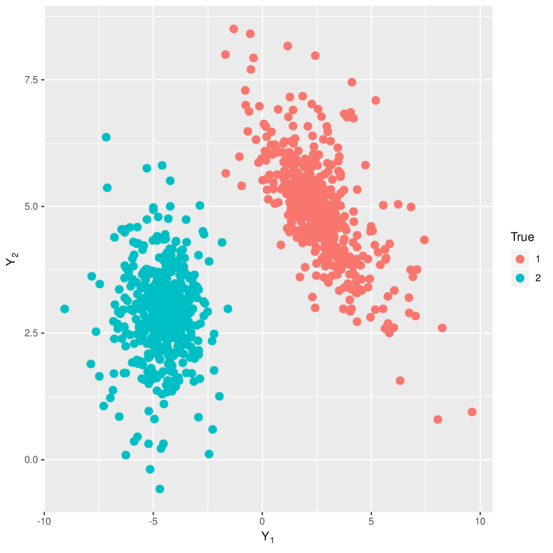
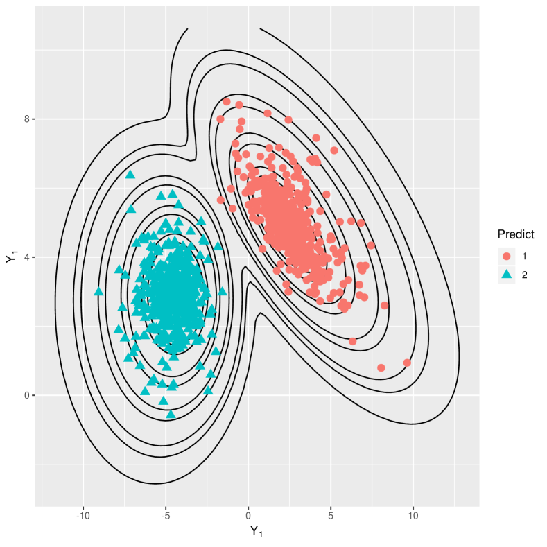
Figure 1: Scatter plot highlighting the true labels (left) and a contour plot showing the predicted classifications (right). Here, the ARI is 1.

Table 1: True and Estimated Values for the MNIG Parameters in Simulation Study 1

	Component 1		Component 2
	True Parameters	Estimated Parameters	True Parameters	Estimated Parameters
		(Standard Error)		(Standard Error)
$\gamma$	$0.9$	$0.97(0.14)$	$1.2$	$1.38(0.19)$
$\delta$	$0.9$	$0.95(0.09)$	$1.2$	$1.33(0.15)$
$\mu$	$[2,\quad 5]$	$[1.96(0.09),\quad 4.99(0.07)]$	$[-4,\quad 3]$	$[-3.90(0.13),\quad 3.00(0.10)]$
$\beta$	$[0.5,\quad 0.5]$	$[0.56(0.10),\quad 0.56(0.13)]$	$[-0.5,\quad-0.1]$	$[-0.75(0.19),\quad-0.14(0.14)]$
$\Delta$	$\begin{bmatrix}2&-1\\ -1&1\end{bmatrix}$	$\begin{bmatrix}1.98(0.11)&-0.99(0.07)\\ -0.99(0.07)&1.00(0.06)\end{bmatrix}$	$\begin{bmatrix}1&0\\ 0&1\end{bmatrix}$	$\begin{bmatrix}1.00(0.06)&-0.01(0.05)\\ -0.01(0.05)&1.00(0.06)\end{bmatrix}$

Figure 1 (left) shows the true component membership of one of the hundred datasets and Figure 1 (right) gives the contour plot based on the estimated parameters for the dataset described in the left panel. Although flexible clustering models based on skewed data have emerged in the last decade or so, Gaussian mixture still remain one of the predominantly used approach for model-based clustering due to its mathematical tractability and the relative computational simplicity with parameter estimation. Therefore, the Gaussian mixture models (GMM) implemented in the R package mclust (Scrucca et al., 2017) are also applied to these datasets. However, these Gaussian mixture models cannot account for skewness. Hence, mixtures of generalized hyperbolic distributions (MixGHD; Browne and McNicholas, 2015) implemented in the R package MixGHD (Tortora et al., 2018) are also applied to these datasets. Mixtures of generalized hyperbolic distributions (McNeil et al., 2015) also have the flexibility of modeling skewed as well as symmetric components. Several skewed distributions such as the skew-$t$ distribution, skew normal distribution, variance-gamma distribution, and MNIG distribution as well as symmetric distributions such as the Gaussian and $t$-distribution can be obtained as a limiting case of the generalized hyperbolic distribution (Browne and McNicholas, 2015). In this simulation, the Gaussian mixture models always chooses 3 or 4 components since it needs more than one component to fit the skew clusters. The mixture of generalized hyperbolic distributions always choose the two-component model as well and gives ARI $=1.00$ with a standard deviation (sd) of $0.00$.

The 95% credible intervals for all parameter estimation for all hundred datasets are given in the Appendix C, where the lower and upper endpoints of the credible intervals are the empirical 0.025-percentiles and 0.975-percentiles.

4.2 Simulation Study 2

In this simulation, 100 four-dimensional datasets were generated with three underlying groups where one component is skewed with 200 observations, the other component is symmetric with 200 observations, and the third component is skewed with 100 observations. The parameters used to generate the data are summarized in Table 2. The proposed algorithm is applied to these datasets for $G=1$ through $G=7$, and it correctly selected the correct three-component model 99 out of 100 times with an average ARI of 1.00 (sd 0.00).

Table 2: True and Estimated Values for the Parameters in Simulation Study 2

	Component 1 ($n=100$)
	True Parameters	Estimated Parameters (Standard Error)
$\gamma$	$0.6$	$0.78(0.19)$
$\delta$	$0.6$	$0.67(0.10)$
$\mu$	$[9,-6,-5,9]$	$[8.95(0.09),-5,96(0.09),-4.95(0.09),8.97(0.09)]$
$\beta$	$[0,0,-0.5,-0.5$	$[-0.10(0.20),0.06(0.19),-0.33(0.21),-0.49(0.26)]$
$\Delta$	$\begin{bmatrix}1&0&0&0\\ 0&1&0&0\\ 0&0&1&0\\ 0&0&0&1\end{bmatrix}$	$\begin{bmatrix}1.03(0.15)&0.01(0.12)&-0.03(0.11)&-0.04(0.11)\\ 0.01(0.12)&1.05(0.15)&0.04(0.13)&0.02(0.11)\\ -0.03(0.11)&0.04(0.13)&1.08(0.15)&0.00(0.13)\\ -0.04(0.11)&0.02(0.11)&0.00(0.13)&0.97(0.12)\end{bmatrix}$
	Component 2 ($n=200$)
	True Parameters	Estimated Parameters (Standard Error)
$\gamma$	$0.9$	$0.94(0.14)$
$\delta$	$0.9$	$0.94(0.09)$
$\mu$	$[5,3,0,-7]$	$[4.96(0.14),2.98(0.09),0.00(0.08),-6.99(0.13)]$
$\beta$	$[0.5,0.5,0.5,0.5]$	$[0.36(0.18),0.47(0.19),0.51(0.22),0.82(0.43)]$
$\Delta$	$\begin{bmatrix}2&0&0&1\\ 0&1&0&0\\ 0&0&1&0\\ 1&0&0&1\end{bmatrix}$	$\begin{bmatrix}2.19(0.25)&0.09(0.11)&0.04(0.14)&1.02(0.16)\\ 0.09(0.11)&1.02(0.11)&0.03(0.09)&0.03(0.09)\\ 0.04(0.14)&0.03(0.09)&1.02(0.10)&0.00(0.09)\\ 1.02(0.16)&0.03(0.09)&0.00(0.09)&0.95(0.12)\end{bmatrix}$
	Component 3 ($n=200$)
	True Parameters	Estimated Parameters (Standard Error)
$\gamma$	$1.2$	$1.40(0.21)$
$\delta$	$1.2$	$1.34(0.16)$
$\mu$	$[-3,-2,7,3]$	$[-2.93(0.13),-1.93(0.13),6.87(0.14),2.93(0.14)]$
$\beta$	$[0,0,0,0]$	$[-0.05(0.16),-0.06(0.15),0.09(0.17),0.06(0.18)]$
$\Delta$	$\begin{bmatrix}1&0&0&0\\ 0&1&0&0\\ 0&0&1&0\\ 0&0&0&1\end{bmatrix}$	$\begin{bmatrix}1.00(0.09)&0.02(0.09)&-0.01(0.08)&0.00(0.08)\\ 0.02(0.09)&1.02(0.10)&0.00(0.09)&0.01(0.08)\\ -0.01(0.08)&0.00(0.09)&1.02(0.11)&0.00(0.09)\\ 0.00(0.08)&0.01(0.08)&0.00(0.09)&1.01(0.09)\end{bmatrix}$

The average of the parameter estimates for the 99 datasets provided in Table 2 shows good parameter recovery. Figure 2 (right) gives the pairwise scatter plot based on the estimated parameters for this dataset where the true group labels are described in the left panel.

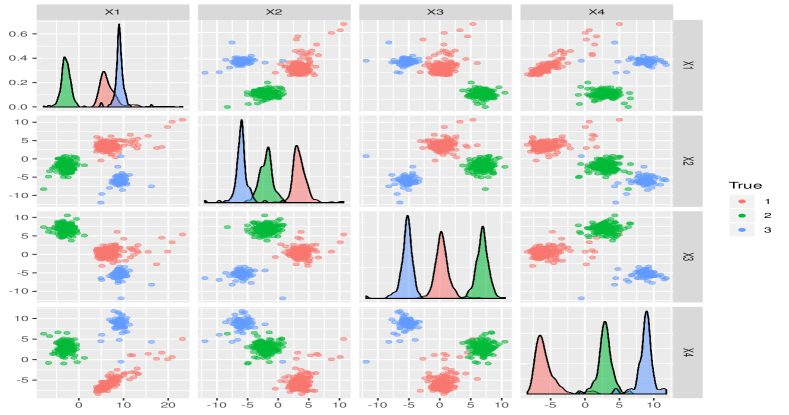
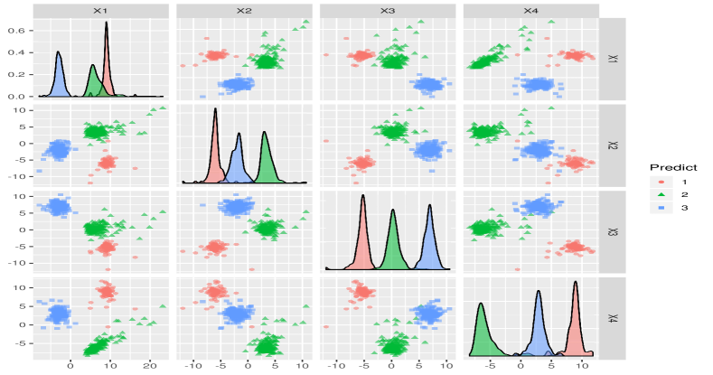
Figure 2: Pairwise scatter plot highlighting the true labels (left) and a pairwise scatter plot showing the predicted classifications (right) of one of the hundred datasets. Here, the ARI was 1.

Gaussian mixture models and mixtures of generalized hyperbolic distributions are applied to these datasets. The mixture of generalized hyperbolic distributions correctly selects the three-component model 84 times out of the 100 datasets with an average ARI of $1.00$ (sd 0.00). The Gaussian mixture models did not choose the correct number of components for all 100 datasets.

4.3 Real Data Analysis

The proposed algorithm is also applied to some benchmark clustering datasets.

The Old Faithful Dataset
The Old Faithful data available in the R package MASS consists of the waiting time between eruptions and the duration of the eruption for the Old Faithful geyser in Yellowstone National Park, Wyoming, USA. There are 272 observations and each observation contains 2 variables (waiting time between eruption and duration of eruption). We ran our algorithm on the scaled data for $G=1~{}\text{to}~{}5$. A two component model was selected. This is consistent with Subedi and McNicholas (2014) that used mixtures of MNIG distributions in a variational Bayes framework and with Franczak et al. (2014) and Vrbik and McNicholas (2012) who used other skewed mixture models. The contour plot of the fitted model given in Figure 3 shows that our fitted model captures the density of the data fairly well.

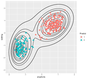
Figure 3: Contour plot for the Old Faithful data using the estimated values of the parameters using the proposed algorithm.

The Fish Catch Dataset
The fish catch data, available from the R package rrcov, consists of the weight and different body lengths measurements of seven different fish species. There are 159 observations in this data set. Similar to Subedi and McNicholas (2014), after dropping the highly correlated variables, the variables Length2, Height and Width were used for the analysis where Length2 is the length from the nose to the notch of the tail, Height is the maximal height as a percentage of the length from the nose to the end of the tail, and Width is the maximal width as a percentage of the length from the nose to the end of the tail. The proposed algorithm is applied (after scaling the data) for $G=1~{}\text{to}~{}9$ and it selects a four-component model. Figure 4 shows the pairwise scatter plots for this dataset, with the left panel showing the true species of the fish and the right panel showing the estimated groups. Although the true number of species of fish is seven, from the pairwise scatter plot one can see that the species White, Roach and Perch are hard to indistinguishable and there is no clear separation between the species Bream and Parkki. Table 3 summarizes the cross tabulation of the true species and estimated group membership and it is consistent with the result from Subedi and McNicholas (2014) that used a variational Bayes approach for clustering using mixtures of MNIG. The GMM and mixGHD are also applied to the Fish Catch data and both resulted in a five component model with classification where the additional fifth component contained fish from both Whitewish and Perch (see Table 3 for detail).

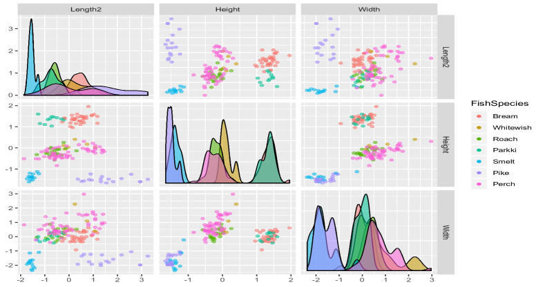
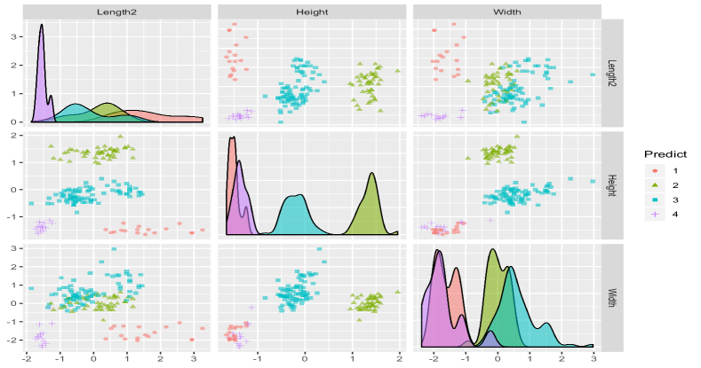
Figure 4: Pairwise scatter plot highlighting the true labels (left) and a pairwise scatter plot showing the predicted classifications (right) for the fish catch data.

Table 3: Cross tabulation of true fish species and the estimated classification using the proposed model, Gaussian mixture models, and the mixtures of generalized hyperbolic distributions.

	Proposed algorithm				GMM					MixGHD
	ARI: 0.63				ARI: 0.52					ARI: 0.54
	Estimated Groups				Estimated Groups					Estimated Groups
	1	2	3	4	1	2	3	4	5	1	2	3	4	5
Bream	34				34								34
Parkki	11				11								11
Whitewish		6				3	3		3			3		3
Roach		20				20						20
Perch		56				36	20		20			36		20
Smelt			14					11	3	14
Pike				17					17		17

The Australian Athletes (AIS) Dataset:
The AIS dataset available in the R package DAAG (Maindonald and Braun, 2019) contains 202 observations and 13 variables comprising of measurements on various characteristics of the blood, body size, and sex of the athlete. The proposed algorithm is applied on a subset of dataset with the variables body mass index (BMI) and body fat (Bfat) as has been previously used (Vrbik and McNicholas, 2012; Lin, 2010). The algorithm is run for $G=1~{}\text{to}~{}5$ and a two-component model is selected. Comparing the estimated component membership with the gender yields an ARI $=0.83$. The contour plot of the fitted model in Figure 5 shows that the fitted model captured the density of the data fairly well. The Gaussian mixture models and mixtures of generalized hyperbolic distributions are also applied to the AIS dataset and the summary of the performance are given in Table 4.The Gaussian mixture model selects a three component model whereas the mixtures of generalized hyperbolic distribution selects a two component model. However, the ARI of the proposed model is higher than that obtained by mixtures of generalized hyperbolic distribution.

Table 4: Summary of the performances of the proposed model, the Gaussian mixture model, and mixtures of generalized hyperbolic distributions on the AIS datasets.

	Estimated Groups	ARI
Proposed Algorithm	$G=2$	0.83
GMM	$G=3$	0.69
MixGHD	$G=2$	0.78

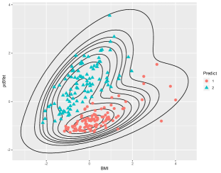
Figure 5: Contour plot using the estimated parameters for the AIS data

The Crab Dataset:
This is dataset of morphological measurements on Leptograpsus crabs, available in the R package MASS (Venables and Ripley, 2002). There are 200 observations and 5 covariates in this dataset, describing 5 morphological measurements on 50 crabs each of two colour forms and both sexes. The five measurements are frontal lobe size (FL), rear width (RW), carapace length (CL), carapace width (CW), and body depth (BD) respectively. All measurements are taken in the unit of millimeters. The proposed algorithm is applied to this dataset for $G=1$ to $G=5$ and it selects a two-component model. Comparison of the estimated group membership with the two color forms of the crabs, “B” or “O” for blue or orange shows complete agreement (ARI$=1$). The pairwise scatter plots are given in Figure 6, where the left panel shows the original measurement variables and the right panel gives the principal components (only for visualization purposes), both colored with estimated classification of the color forms.

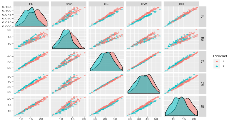
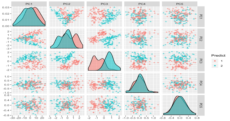
Figure 6: Pairwise scatter plot highlighting the predicted classification of the color forms of the crabs, in terms of the original measurements (left), and in terms of the principal components (right).

The Gaussian mixture models and the mixtures of generalized hyperbolic distributions are also applied to this dataset and the performance is summarized in Table 5.

Table 5: Summary of the performances of the proposed model, the Gaussian mixture model, and mixtures of generalized hyperbolic distributions on the crabs datasets.

	Model Chosen	ARI (color)	ARI (gender)
GMM	$G=3$	0.02	0.72
MixGHD	$G=2$	0.00	0.77
Proposed Algorithm	$G=2$	1.00	0.00

The mixtures of generalized hyperbolic distributions selects a two-component model (see Table 5). However, the estimated group membership are more in agreement with classifying the crabs by their sexes (ARI of 0.77). The Gaussian mixture model on the other hand yielded a three component model where the classification obtained are also more in agreement with the classification based on the sex of the crabs (ARI of 0.72) (see Table 5).

5 Conclusion

In summary, we proposed a fully Bayesian approach for parameter estimation for mixtures of MNIG distributions. We also propose novel approaches to simulate from two distributions: GIG distributions and MGIG distributions. Through simulation studies, we show that the parameter estimates were very close to the true parameters and close to perfect classification was obtained. In simulation studies, the correct number of components were always selected using BIC. Using both simulated and real datasets, we show that our approach provides competitive clustering results compared to other clustering approaches. The contour plots using the estimated parameters show that the mixture distribution captures the shape of the dataset closely.

When the true number of groups is unknown which is typically the case, the optimal number of components is chosen a posteriori using a model selection criterion. At present, the BIC is most popular but different model selection can choose different models and the BIC does not always choose the best one. In our case, the model selection using BIC seemed to perform fairly well in both simulated and real data analysis. However, the search for a highly effective model selection criteria remains an open problem especially when dealing with skewed data.

Appendix

Appendix A The matrix-GIG distribution

The MGIG was introduced by Barndorff-Nielsen et al. (1982). Let $\mathcal{V}_{n}$ be the Euclidean space of $n\times n$ real symmetric matrices. Let also $\mathcal{V}_{n}^{+}$ denote the cone of positive definite matrices in $\mathcal{V}_{n}$.

A random matrix ${\bf X}$ taking its values in $\mathcal{V}_{n}^{+}$ is said to follow the $MGIG_{n}(-p,a,b)$ distribution if it has density of the form

$$f_{\bf X}({\bf x})\propto|{\bf x}|^{-p-\frac{n+1}{2}}\exp\left(-Tr(a{\bf x})-Tr(b{\bf x}^{-1})\right)$$

The above density is well defined if $a,b\in\mathcal{V}_{n}^{+}$ and $p\in\cal{R}$. According to Massam and Wesolowski (2006), the density is well defined for non positive definite matrices $a$ and $b$ if certain conditions hold, but these cases are not of interest for our purpose.

Similarly, a random matrix ${\bf X}$ taking its values in $\mathcal{V}_{n}^{+}$ is said to follow the Wishart (denoted as $W_{n}(q,c)$) distribution if it has density of the form

$$f_{X}(x)\propto|x|^{q-\frac{n+1}{2}}\exp\left(-Tr(cx)\right)$$

were $c\in\mathcal{V}_{n}^{+}$, $q>(n-1)/2$.

Appendix B Mathematical Details for Posterior Distributions

$$\begin{split}&f_{U_{ig}}(u|\mathbf{Y}_{i}=\mathbf{y}_{i})\propto f_{\mathbf{Y}}(\mathbf{Y}|U=u)f_{U}(u)\\ &\propto u^{-\frac{d+3}{2}}\exp\left\{-\frac{1}{2}\left(\frac{\delta_{g}^{2}}{u}+\gamma_{g}^{2}u\right)-\frac{1}{2}(\mathbf{y}_{i}-\mbox{\boldmath{$\mu$}}_{g}-u\mbox{\boldmath{$\Delta$}}_{g}\mbox{\boldmath{$\beta$}}_{g})(u\mbox{\boldmath{$\Delta$}}_{g})^{-1}(\mathbf{y}_{i}-\mbox{\boldmath{$\mu$}}_{g}-u\mbox{\boldmath{$\Delta$}}_{g}\mbox{\boldmath{$\beta$}}_{g})^{\top}\right\}\\ &=u^{-\frac{d+3}{2}}\exp\left\{-\frac{1}{2}\left(\frac{\delta_{g}^{2}}{u}+\gamma_{g}^{2}u\right)-\frac{1}{2}\left[\left((\mathbf{y}_{i}-\mbox{\boldmath{$\mu$}}_{g})\mbox{\boldmath{$\Delta$}}^{-1}(\mathbf{y}_{i}-\mbox{\boldmath{$\mu$}}_{g})^{\top}\right)u^{-1}+(\mbox{\boldmath{$\beta$}}_{g}\mbox{\boldmath{$\Delta$}}_{g}\mbox{\boldmath{$\beta$}}_{g}^{\top})u\right]\right\}\\ &=u^{-\frac{d+3}{2}}\exp\left\{-\frac{1}{2}\left(\frac{\delta_{g}^{2}+(\mathbf{y}_{i}-\mbox{\boldmath{$\mu$}}_{g})\mbox{\boldmath{$\Delta$}}^{-1}(\mathbf{y}_{i}-\mbox{\boldmath{$\mu$}}_{g})^{\top}}{u}+(\gamma_{g}^{2}+\mbox{\boldmath{$\beta$}}_{g}\mbox{\boldmath{$\Delta$}}_{g}\mbox{\boldmath{$\beta$}}_{g}^{\top})u\right)\right\}\\ &=u^{-\frac{d+3}{2}}\exp\left\{-\frac{1}{2}\left(\frac{q^{2}(\mathbf{y}_{i})}{u}+\alpha_{g}^{2}u\right)\right\}.\end{split}$$

Therefore, the posterior distribution of $U_{ig}|\mathbf{Y}_{i}$ are the $\mathop{\rm GIG}$ distributions:

$$\begin{split}U_{ig}|\mathbf{Y}_{i}=\mathbf{y}_{i}&\sim\mathop{\rm GIG}\left(\frac{d+1}{2},q^{2}(\mathbf{y}_{i}),\alpha_{g}^{2}\right),\\ U_{ig}^{-1}|\mathbf{Y}_{i}=\mathbf{y}_{i}&\sim\mathop{\rm GIG}\left(-\frac{d+1}{2},\alpha_{g}^{2},q^{2}(\mathbf{y}_{i})\right).\end{split}$$

The contribution from $\left(\delta_{g},\gamma_{g}\right)$ to the likelihood is given as follows:

$$f(\delta_{g},\gamma_{g}|\cdot)\propto\delta_{g}^{2\cdot\frac{1}{2}\sum_{i}{z_{ig}}}\times\exp\left\{\delta_{g}\gamma_{g}\sum_{i}{z_{ig}}+\frac{1}{2}\left(\gamma_{g}^{2}\sum_{i=1}^{n}{z_{ig}u_{ig}}+\delta_{g}^{2}\sum_{i=1}^{n}{z_{ig}u_{ig}^{-1}}\right)\right\}.$$

Given the prior of $\delta_{g}^{2}$ of the form

$$\delta_{g}^{2}\sim Gamma\left(\frac{a_{g,0}^{(0)}}{2}+1,a_{g,4}^{(0)}-\frac{{a^{(0)}_{g,0}}^{2}}{4a_{g,3}^{(0)}}\right),$$

the posterior distribution of $\delta_{g}^{2}$ is derived as below:

$$\begin{split}f(\delta_{g}^{2}|\cdot)\propto&{\delta_{g}}^{2\cdot\frac{1}{2}\sum_{i}{z_{ig}}}\cdot\exp\left\{\delta_{g}\gamma_{g}\sum_{i}{z_{ig}}+\frac{1}{2}\delta_{g}^{2}\left(\sum_{i=1}^{n}{z_{ig}u_{ig}^{-1}}\right)\right\}\\ &\times\left(\delta_{g}^{2}\right)^{a_{g,0}^{(0)}/2+1}\cdot\exp\left\{-\delta_{g}^{2}\left(a_{g,4}^{(0)}-\frac{{a^{(0)}_{g,0}}^{2}}{4a_{g,3}}\right)\right\}\\ =&(\delta_{g}^{2})^{a_{g,0}/2+1}\times\exp\left\{-\delta_{g}^{2}\left(a_{g,4}^{(0)}-\frac{{a^{(0)}_{g,0}}^{2}}{4a_{g,3}^{(0)}}\right)\right\}.\\ \end{split}$$

which indicates that the posterior distribution of $\delta_{g}^{2}$ is

$$\delta_{g}^{2}\sim Gamma\left(\frac{a_{g,0}}{2}+1,a_{g,4}-\frac{{a_{g,0}}^{2}}{4a_{g,3}}\right).$$

Conditional on $\delta_{g}$, a truncated Normal conjugate prior is assigned to $\gamma_{g}$. The resulting posterior distribution is given as:

$$\gamma_{g}|\delta_{g}\sim\mathop{\rm N}\left(\dfrac{a_{g,0}\delta_{g}}{2a_{g,3}},\dfrac{1}{2a_{g,3}}\right)\cdot\mathbf{1}\left(\gamma_{g}>0\right).$$

Conjugate joint multivariate normal prior conditional on $\mbox{\boldmath{$\Delta$}}_{g}$ was assigned to $(\mbox{\boldmath{$\mu$}}_{g},\mbox{\boldmath{$\beta$}}_{g})$, i.e.,

$$\left.\begin{pmatrix}\mbox{\boldmath{$\mu$}}_{g}\\ \mbox{\boldmath{$\beta$}}_{g}\end{pmatrix}\right|\mbox{\boldmath{$\Delta$}}_{g}\sim MVN\left[\begin{pmatrix}\mbox{\boldmath{$\mu$}}_{0}\\ \mbox{\boldmath{$\beta$}}_{0}\end{pmatrix},\begin{pmatrix}\mbox{\boldmath{$\Sigma$}}_{\mu_{0}}&\mbox{\boldmath{$\Sigma$}}_{\mu_{0},\beta_{0}}\\ \mbox{\boldmath{$\Sigma$}}_{\mu_{0},\beta_{0}}&\mbox{\boldmath{$\Sigma$}}_{\beta_{0}}\end{pmatrix}\right],$$

where
$\mbox{\boldmath{$\mu$}}_{0}=\dfrac{2\mathbf{a}_{g,2}^{(0)}a_{g,3}^{(0)}-a_{g,0}^{(0)}\mathbf{a}_{1}^{(0)}}{4a_{g,3}^{(0)}a_{g,4}^{(0)}-{a^{(0)}_{g,0}}^{2}}$, $\mbox{\boldmath{$\beta$}}_{0}=\dfrac{\mbox{\boldmath{$\Delta$}}_{g}^{-1}(2\mathbf{a}_{g,1}^{(0)}a_{g,4}^{(0)}-a_{g,0}^{(0)}\mathbf{a}_{g,2}^{(0)})}{4a_{g,3}^{(0)}a_{g,4}^{(0)}-{a^{(0)}_{g,0}}^{2}}$, $\mbox{\boldmath{$\Sigma$}}_{\mu_{0}}=\dfrac{2a_{g,3}^{(0)}\mbox{\boldmath{$\Delta$}}_{g}}{4a_{g,3}^{(0)}a_{g,4}^{(0)}-{a^{(0)}_{g,0}}^{2}},\\ \mbox{\boldmath{$\Sigma$}}_{\beta_{0}}=\dfrac{2a_{g,4}^{(0)}\mbox{\boldmath{$\Delta$}}^{-1}_{g}}{4a_{g,3}^{(0)}a_{g,4}^{(0)}-{a^{(0)}_{g,0}}^{2}}$ and $\mbox{\boldmath{$\Sigma$}}_{\mu_{0},\beta_{0}}=\dfrac{-a_{g,0}^{(0)}\mathbb{I}_{d}}{4a_{g,3}^{(0)}a_{g,4}^{(0)}-{a^{(0)}_{g,0}}^{2}}$.

Therefore, the posterior should be a joint multivariate normal distribution as well of the form

$$\left.\begin{pmatrix}\mbox{\boldmath{$\mu$}}_{g}\\ \mbox{\boldmath{$\beta$}}_{g}\end{pmatrix}\right|\cdot\sim MVN\left[\begin{pmatrix}\mbox{\boldmath{$\mu$}}^{*}\\ \mbox{\boldmath{$\beta$}}^{*}\end{pmatrix},\begin{pmatrix}\mbox{\boldmath{$\Sigma$}}_{\mu}&\mbox{\boldmath{$\Sigma$}}_{\mu,\beta}\\ \mbox{\boldmath{$\Sigma$}}_{\mu,\beta}&\mbox{\boldmath{$\Sigma$}}_{\beta}\end{pmatrix}\right].$$

The joint density of $(\mbox{\boldmath{$\mu$}}_{g},\mbox{\boldmath{$\beta$}}_{g})$ from the likelihood is given as follows:

$$\begin{split}f(\mbox{\boldmath{$\mu$}}_{g},\mbox{\boldmath{$\beta$}}_{g}\mid\cdot)\propto&\exp\left\{\left(-\mbox{\boldmath{$\beta$}}_{g}^{\top}\mbox{\boldmath{$\mu$}}_{g}\right)\sum_{i}{z_{ig}}+\mbox{\boldmath{$\beta$}}_{g}^{\top}\sum_{i=1}^{n}{z_{ig}\mathbf{y}_{i}}+\mbox{\boldmath{$\mu$}}_{g}^{\top}\mbox{\boldmath{$\Delta$}}_{g}^{-1}\sum_{i=1}^{n}{z_{ig}u_{ig}^{-1}\mathbf{y}_{i}}\right.\\ &\left.\quad\quad-\frac{1}{2}\left[\mbox{\boldmath{$\beta$}}_{g}^{\top}\left(\sum_{i=1}^{n}{u_{ig}z_{ig}}\right)\mbox{\boldmath{$\Delta$}}_{g}\mbox{\boldmath{$\beta$}}_{g}\right]-\frac{1}{2}\left[\mbox{\boldmath{$\mu$}}_{g}^{\top}\left(\sum_{i=1}^{n}{u_{ig}^{-1}z_{ig}}\right)\mbox{\boldmath{$\Delta$}}_{g}^{-1}\mbox{\boldmath{$\mu$}}_{g}\right]\right\}.\\ \end{split}$$

Hence, the marginal density of $\mbox{\boldmath{$\mu$}}_{g}$ and $\mbox{\boldmath{$\beta$}}_{g}$ from the posterior are given as the following:

$$\begin{split}f(\mbox{\boldmath{$\mu$}}_{g}|\mbox{\boldmath{$\beta$}}_{g}=\mbox{\boldmath{$\beta$}}_{0},\mbox{\boldmath{$\Delta$}}_{g})\propto&\exp\left\{-\frac{1}{2}\left[\mbox{\boldmath{$\mu$}}_{g}^{\top}(2a_{g,4}\mbox{\boldmath{$\Delta$}}_{g}^{-1})\mbox{\boldmath{$\mu$}}_{g}-\mbox{\boldmath{$\mu$}}_{g}^{\top}\left(\mbox{\boldmath{$\Delta$}}_{g}^{-1}\mathbf{a}_{g,2}-a_{g,0}\mbox{\boldmath{$\beta$}}_{g}\right)\right.\right.\\ &-\left(\mbox{\boldmath{$\Delta$}}_{g}^{-1}\mathbf{a}_{g,2}-a_{g,0}\mbox{\boldmath{$\beta$}}_{0}\right)^{\top}\mbox{\boldmath{$\mu$}}_{g}\\ &\left.\left.+\left(\mbox{\boldmath{$\Delta$}}_{g}^{-1}\mathbf{a}_{g,2}-a_{g,0}\mbox{\boldmath{$\beta$}}_{0}\right)^{\top}\left(\frac{\mbox{\boldmath{$\Delta$}}_{g}}{2a_{g,4}}\right)\left(\mbox{\boldmath{$\Delta$}}_{g}^{-1}\mathbf{a}_{g,2}-a_{g,0}\mbox{\boldmath{$\beta$}}_{0}\right)\right]\right\},\\ f(\mbox{\boldmath{$\beta$}}_{g}|\mbox{\boldmath{$\mu$}}_{g}=\mbox{\boldmath{$\mu$}}_{0},\mbox{\boldmath{$\Delta$}}_{g})\propto&\exp\left\{-\frac{1}{2}\left[\mbox{\boldmath{$\beta$}}_{g}^{\top}(2a_{g,3}\mbox{\boldmath{$\Delta$}}_{g})\mbox{\boldmath{$\beta$}}_{g}-\mbox{\boldmath{$\beta$}}_{g}^{\top}\left(\mathbf{a}_{g,1}-a_{g,0}\mbox{\boldmath{$\mu$}}_{0}\right)\right.\right.\\ &\left.\left.\quad-\left(\mathbf{a}_{g,1}-a_{g,0}\mbox{\boldmath{$\mu$}}_{0}\right)^{\top}\mbox{\boldmath{$\beta$}}_{g}+\left(\mathbf{a}_{g,1}-a_{g,0}\mbox{\boldmath{$\mu$}}_{0}\right)^{\top}\left(\frac{\mbox{\boldmath{$\Delta$}}_{g}^{-1}}{2a_{3}}\right)\left(\mathbf{a}_{g,1}-a_{g,0}\mbox{\boldmath{$\mu$}}_{0}\right)\right]\right\}.\\ \end{split}$$

Based on the conditional normal property of the multivariate normal variables,

$$\begin{split}\left(\mbox{\boldmath{$\mu$}}_{g}|\mbox{\boldmath{$\beta$}}_{g}=\mbox{\boldmath{$\beta$}}_{0},\mbox{\boldmath{$\Delta$}}_{g},\cdot\right)&\sim MVN\left(\mbox{\boldmath{$\mu$}}^{*}+\mbox{\boldmath{$\Sigma$}}_{\mu,\beta}\mbox{\boldmath{$\Sigma$}}_{\beta}^{-1}(\mbox{\boldmath{$\beta$}}_{0}-\mbox{\boldmath{$\beta$}}^{*}),\mbox{\boldmath{$\Sigma$}}_{\mu}-\mbox{\boldmath{$\Sigma$}}_{\mu,\beta}\mbox{\boldmath{$\Sigma$}}_{\beta}^{-1}\mbox{\boldmath{$\Sigma$}}_{\mu,\beta}\right)\quad\text{and}\\ \left(\mbox{\boldmath{$\beta$}}_{g}|\mbox{\boldmath{$\mu$}}_{g}=\mbox{\boldmath{$\mu$}}_{0},\mbox{\boldmath{$\Delta$}}_{g},\cdot\right)&\sim MVN\left(\mbox{\boldmath{$\beta$}}^{*}+\mbox{\boldmath{$\Sigma$}}_{\mu,\beta}\mbox{\boldmath{$\Sigma$}}_{\mu}^{-1}(\mbox{\boldmath{$\mu$}}_{0}-\mbox{\boldmath{$\mu$}}^{*}),\mbox{\boldmath{$\Sigma$}}_{\beta}-\mbox{\boldmath{$\Sigma$}}_{\mu,\beta}\mbox{\boldmath{$\Sigma$}}_{\mu}^{-1}\mbox{\boldmath{$\Sigma$}}_{\mu,\beta}\right),\end{split}$$

we can derive that

$$\mbox{\boldmath{$\mu$}}^{*}=\dfrac{2\mathbf{a}_{g,2}a_{g,3}-a_{g,0}\mathbf{a}_{1}}{4a_{g,3}a_{g,4}-{a_{g,0}}^{2}}\quad\quad\mbox{\boldmath{$\beta$}}^{*}=\dfrac{\mbox{\boldmath{$\Delta$}}_{g}^{-1}(2\mathbf{a}_{g,1}a_{g,4}-a_{g,0}\mathbf{a}_{g,2})}{4a_{g,3}a_{g,4}-{a_{g,0}}^{2}},$$

$$\mbox{\boldmath{$\Sigma$}}_{\mu}=\dfrac{2a_{g,3}\mbox{\boldmath{$\Delta$}}_{g}}{4a_{g,3}a_{g,4}-{a_{g,0}}^{2}},\quad\mbox{\boldmath{$\Sigma$}}_{\beta}=\dfrac{2a_{g,4}\mbox{\boldmath{$\Delta$}}^{-1}_{g}}{4a_{g,3}a_{g,4}-{a_{g,0}}^{2}},\quad\mbox{\boldmath{$\Sigma$}}_{\mu,\beta}=\dfrac{-a_{g,0}\mathbb{I}_{d}}{4a_{g,3}a_{g,4}-{a_{g,0}}^{2}}.$$

An Inverse-Wishart prior is given to $\mbox{\boldmath{$\Delta$}}_{g}$, the resulting posterior is a Matrix Generalized Inverse-Gaussian (MGIG) distribution. The derivation is given as below:

$$\begin{split}&f(\mbox{\boldmath{$\Delta$}}_{g}|\cdot)\propto|\mbox{\boldmath{$\Delta$}}_{g}|^{-\frac{\sum_{i}{z_{ig}}}{2}}\times\exp Tr\left\{-\mbox{\boldmath{$\beta$}}_{g}\left(\frac{1}{2}\sum_{i=1}^{n}{u_{ig}z_{ig}}\right)\mbox{\boldmath{$\beta$}}_{g}^{\top}\mbox{\boldmath{$\Delta$}}_{g}-\sum_{i=1}^{n}{\frac{(\mathbf{y}_{i}-\mbox{\boldmath{$\mu$}}_{g})(\mathbf{y}_{i}-\mbox{\boldmath{$\mu$}}_{g})^{\top}}{2u_{i}}}\mbox{\boldmath{$\Delta$}}_{g}^{-1}\right\}\\ &\times|\mbox{\boldmath{$\Delta$}}_{g}|^{-\frac{\nu_{0}+d+1}{2}}\times\exp Tr\left\{-\frac{1}{2}\Lambda_{0}\mbox{\boldmath{$\Delta$}}_{g}^{-1}\right\}\\ =&|\mbox{\boldmath{$\Delta$}}_{g}|^{-\frac{t_{g,0}+\nu_{0}+d+1}{2}}\times\exp Tr\left\{-\frac{1}{2}\mbox{\boldmath{$\beta$}}_{g}\mbox{\boldmath{$\beta$}}_{g}^{\top}(2t_{g,3})\mbox{\boldmath{$\Delta$}}_{g}-\frac{1}{2}\left(\sum_{i=1}^{n}{z_{ig}u_{ig}^{-1}(\mathbf{y}_{i}-\mbox{\boldmath{$\mu$}}_{g})(\mathbf{y}_{i}-\mbox{\boldmath{$\mu$}}_{g})^{\top}}+\Lambda_{0}\right)\mbox{\boldmath{$\Delta$}}_{g}^{-1}\right\}\\ =&|\mbox{\boldmath{$\Delta$}}_{g}|^{-\frac{t_{g,0}+\nu_{0}+d+1}{2}}\times\exp Tr\left\{-\frac{1}{2}\mbox{\boldmath{$\beta$}}_{g}\mbox{\boldmath{$\beta$}}_{g}^{\top}(2t_{g,3})\mbox{\boldmath{$\Delta$}}_{g}-\frac{1}{2}\left({S_{0}}_{g}+\Lambda_{0}\right)\mbox{\boldmath{$\Delta$}}_{g}^{-1}\right\}.\\ \end{split}$$

Therefore, the posterior of $\mbox{\boldmath{$\Delta$}}_{g}$ is

$$\mbox{\boldmath{$\Delta$}}_{g}\sim MGIG_{d}\left(-\frac{\nu_{0}+t_{0g}}{2},\mbox{\boldmath{$\beta$}}_{g}2t_{3g}\mbox{\boldmath{$\beta$}}_{g}^{\top},{S_{0}}_{g}+\Lambda_{0}\right).$$

Appendix C Credible Intervals for Simulation Study 1

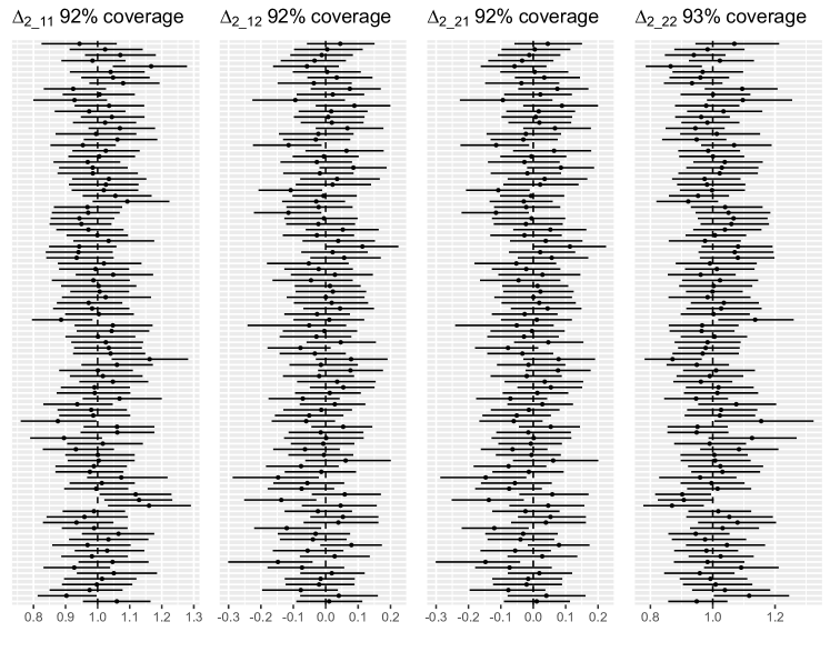
Figure 7: 95% Credible Intervals for estimated parameters for all 100 runs for Simulation Study 1.

References

- Akaike (1983) Akaike, H. (1983), “Information Measures and Model Selection,” In Proceedings of the International Statistical Institute 44th Session, 277–291.
- Atkinson (1982) Atkinson, A. (1982), “The simulation of generalized inverse Gaussian and hyperbolic random variables,” SIAM Journal on Scientific and Statistical Computing, 3, 502–515.
- Barndorff-Nielsen et al. (1982) Barndorff-Nielsen, O., Blaesild, P., Jensen, J. L., and Jørgensen, B. (1982), “Exponential transformation models,” Proceedings of the Royal Society of London. A. Mathematical and Physical Sciences, 379, 41–65.
- Barndorff-Nielsen (1997) Barndorff-Nielsen, O. E. (1997), “Normal inverse Gaussian distributions and stochastic volatility modelling,” Scandinavian Journal of Statistics, 24, 1–13.
- Biernacki et al. (1998) Biernacki, C., Celeux, G., and Govaert, G. (1998), “Assessing a Mixture Model for Clustering with the Integrated Classification Likelihood,” Tech. rep., Institut National de Recherche en informatique et en automatique.
- Blei et al. (2017) Blei, D. M., Kucukelbir, A., and McAuliffe, J. D. (2017), “Variational inference: A review for statisticians,” Journal of the American Statistical Association, 112, 859–877.
- Browne and McNicholas (2015) Browne, R. P., and McNicholas, P. D. (2015), “A mixture of generalized hyperbolic distributions,” The Canadian Journal of Statistics, 43, 176–198.
- Celeux et al. (2000) Celeux, G., Hurn, M., and Robert, C. P. (2000), “Computational and Inferential Difficulties with Mixture Posterior Distributions,” Journal of the American Statistical Association, 95, 957–970.
- Dagpunar (1989) Dagpunar, J. (1989), “An Easily Implemented Generalised Inverse Gaussian Generator,” Communications in Statistics - Simulation and Computation, 18, 703–710.
- Devroye (2014) Devroye, L. (2014), “Random variate generation for the generalized inverse Gaussian distribution,” Statistics and Computing, 24, 239–246.
- Diebolt and Robert (1994) Diebolt, J., and Robert, C. P. (1994), “Estimation of finite mixture distributions through Bayesian sampling,” Journal of the Royal Statistical Society: Series B (Methodology), 56, 363–375.
- Fazayeli and Banerjee (2016) Fazayeli, F., and Banerjee, A. (2016), in Machine Learning and Knowledge Discovery in Databases, eds. Frasconi, P., Landwehr, N., Manco, G., and Vreeken, J., Cham: Springer International Publishing, pp. 648–664.
- Fraley and Raftery (2002) Fraley, C., and Raftery, A. E. (2002), “Model-Based Clustering, Discriminant Analysis, and Density Estimation,” Journal of the American Statistical Association, 97, 611–631.
- Franczak et al. (2014) Franczak, B. C., Browne, R. P., and McNicholas, P. D. (2014), “Mixtures of shifted asymmetric Laplace distributions,” IEEE Transactions on Pattern Analysis and Machine Intelligence, 36, 1149–1157.
- Frühwirth-Schnatter (2006) Frühwirth-Schnatter, S. (2006), Finite mixture and Markov switching models, Springer Science & Business Media.
- Fruhwirth-Schnatter and Pyne (2010) Fruhwirth-Schnatter, S., and Pyne, S. (2010), “Bayesian Inference for finite mixtures of univatiate and multivariate skew-normal and skew-t distributions,” Biostatistics, 11, 317–336.
- Gelman et al. (2013) Gelman, A., Carlin, J. B., Stern, H. S., Dunson, D. B., Vehtari, A., and Rubin, D. B. (2013), Bayesian Data Analysis, CRC Press, 3rd ed.
- Gelman et al. (1992) Gelman, A., Rubin, D. B. et al. (1992), “Inference from iterative simulation using multiple sequences,” Statistical Science, 7, 457–472.
- Goswami (2004) Goswami, A. (2004), “Random Continued Fractions: A Markov Chain Approach,” Economic Theory, 23, 85–105.
- Hejblum et al. (2019) Hejblum, B. P., Alkhassim, C., Gottardo, R., Caron, F., Thiébaut, R. et al. (2019), “Sequential Dirichlet process mixtures of multivariate skew -distributions for model-based clustering of flow cytometry data,” The Annals of Applied Statistics, 13, 638–660.
- Hörmann and Leydold (2014) Hörmann, W., and Leydold, J. (2014), “Generating generalized inverse Gaussian random variates,” Statistics and Computing, 24, 547–557.
- Hubert and Arabie (1985) Hubert, L., and Arabie, P. (1985), “Comparing partitions,” Journal of Classification, 2, 193–218.
- Karlis and Santourian (2009) Karlis, D., and Santourian, A. (2009), “Model-based clustering with non-elliptically contoured distributions,” Statistics and Computing, 19, 73–83.
- Keribin (2000) Keribin, C. (2000), “Consistent Estimation of the Order of Mixture Models,” Sankhya: The Indian Journal of Statistics, Series A, 62, 49–66.
- Lai (2009) Lai, Y. (2009), “Generating inverse Gaussian random variates by approximation,” Computational Statistics & Data Analysis, 53, 3553–3559.
- Leroux (1992) Leroux, B. G. (1992), “Consistent Estimation of a Mixing Distribution,” The Annals of Statistics, 20, 1350–1360.
- Letac and Seshadri (1983) Letac, G., and Seshadri, V. (1983), “A characterization of the generalized inverse Gaussian distribution by continued fractions,” Probability Theory and Related Fields, 62, 485–489.
- Letac and Wesołowski (2000) Letac, G., and Wesołowski, J. (2000), “An independence property for the product of GIG and gamma laws,” The Annals of Probability, 28, 1371–1383.
- Leydold and Hörmann (2011) Leydold, J., and Hörmann, W. (2011), “Generating generalized inverse Gaussian random variates by fast inversion,” Computational Statistics & Data Analysis, 55, 213–217.
- Lin (2010) Lin, T. I. (2010), “Robust mixture modeling using multivariate skew distributions,” Statistics and Computing, 20, 343–356.
- Lin et al. (2007a) Lin, T. I., Lee, J. C., and Hsieh, W. J. (2007a), “Robust mixture modeling using the skew distribution,” Statistics and Computing, 17, 81–92.
- Lin et al. (2007b) Lin, T. I., Lee, J. C., and Yen, S. Y. (2007b), “Finite mixture modeling using the skew normal distribution,” Statistica Sinica, 17, 909–927.
- Maindonald and Braun (2019) Maindonald, J. H., and Braun, W. J. (2019), DAAG: Data Analysis and Graphics Data and Functions, r package version 1.22.1.
- Maleki et al. (2019) Maleki, M., Wraith, D., and Arellano-Valle, R. B. (2019), “Robust finite mixture modeling of multivariate unrestricted skew-normal generalized hyperbolic distributions,” Statistics and Computing, 29, 415–428.
- Massam and Wesolowski (2006) Massam, H., and Wesolowski, J. (2006), “The Matsumoto-Yor property and the structure of the Wishart distribution,” Journal of Multivariate Analysis, 97, 103–123.
- McNeil et al. (2015) McNeil, A. J., Frey, R., Embrechts, P. et al. (2015), “Quantitative risk management: Concepts,” Economics Books.
- McNicholas et al. (2017) McNicholas, S. M., McNicholas, P. D., and Browne, R. P. (2017), “A mixture of variance-gamma factor analyzers,” in Big and Complex Data Analysis, Springer, pp. 369–385.
- Murray et al. (2014) Murray, P. M., Browne, R. P., and McNicholas, P. D. (2014), “Mixtures of skew- factor analyzers,” Computational Statistics & Data Analysis, 77, 326–335.
- O’Hagan et al. (2016) O’Hagan, A., Murphy, T. B., Gormley, I. C., McNicholas, P. D., and Karlis, D. (2016), “Clustering with the multivariate normal inverse Gaussian distribution,” Computational Statistics & Data Analysis, 93, 18–30.
- Pyne et al. (2009) Pyne, S., Hu, X., Wang, K., Rossin, E., Lin, T.-I., Baecher-Allan, L. M. M. C., McLachlan, G. J., Tamayo, P., Hafler, D. A., Jager, P. L. D., and Mesirov, J. P. (2009), “Automated high-dimensional flow cytometric data analysis,” Proceedings of the National Academy of Sciences, 106, 8519–8524.
- Richarson and Green (1997) Richarson, S., and Green, P. J. (1997), “On Bayesian analysis of mixtures with an unknown number of components,” Journal of the Royal Statistical Society: Series B (Methodology), 59, 731–792.
- Robert (1996) Robert, C. P. (1996), “Mixtures of distributions: inference and estimation,” Markov chain Monte Carlo in practice, 441, 464.
- Roeder and Wasserman (1997) Roeder, K., and Wasserman, L. (1997), “Practical Bayesian Density Estimation Using Mixtures of Normals,” Journal of the American Statistical Association, 92, 894–902.
- Schwarz (1978) Schwarz, G. (1978), “Estimating the Dimension of a Model,” The Annals of Statistics, 6, 461–464.
- Scrucca et al. (2017) Scrucca, L., Fop, M., Murphy, T. B., and Raftery, A. E. (2017), “mclust 5: clustering, classification and density estimation using Gaussian finite mixture models,” The R Journal, 8, 205–233.
- Spiegelhalter et al. (2002) Spiegelhalter, D. J., Best, N. G., Carlin, B. P., and Linde, A. V. D. (2002), “Bayesian measures of model complexity and fit,” Journal of the Royal Statistical Society, Series B (Methodology), 64, 583–616.
- Steel and Raftery (2009) Steel, R. J., and Raftery, A. E. (2009), “Performance of Bayesian Model Selection Criteria for Gaussian Mixture Models,” Tech. rep., Department of Statistics University of Washington.
- Stephens (2000) Stephens, M. (2000), “Dealing with Label Switching in Mixture Models,” Journal of Royal Statistical Society. Series B (Methodology), 62, 795–809.
- Stephens et al. (2000) Stephens, M. et al. (2000), “Bayesian analysis of mixture models with an unknown number of components - an alternative to reversible jump methods,” The Annals of Statistics, 28, 40–74.
- Subedi and McNicholas (2014) Subedi, S., and McNicholas, P. D. (2014), “Variational Bayes approximations for clustering via mixtures of normal inverse Gaussian distributions,” Advances in Data Analysis and Classification, 8, 167–193.
- Titterington et al. (1985) Titterington, D. M., Smith, A. F., and Makov, U. E. (1985), Statistical analysis of finite mixture distributions, Wiley,.
- Tortora et al. (2018) Tortora, C., ElSherbiny, A., Browne, R. P., Franczak, B. C., , McNicholas, P. D., and D.., A. D. (2018), MixGHD: Model Based Clustering, Classification and Discriminant Analysis Using the Mixture of Generalized Hyperbolic Distributions, r package version 2.2.
- Venables and Ripley (2002) Venables, W. N., and Ripley, B. D. (2002), Modern Applied Statistics with S, New York: Springer, 4th ed., iSBN 0-387-95457-0.
- Vrbik and McNicholas (2012) Vrbik, I., and McNicholas, P. (2012), “Analytic calculations for the EM algorithm for multivariate skew- mixture models,” Statistics & Probability Letters, 82, 1169–1174.
- Wei et al. (2019) Wei, Y., Tang, Y., and McNicholas, P. D. (2019), “Mixtures of generalized hyperbolic distributions and mixtures of skew- distributions for model-based clustering with incomplete data,” Computational Statistics & Data Analysis, 130, 18–41.