Differentiable Greedy Submodular Maximization: Guarantees, Gradient Estimators, and Applications

Abstract

Motivated by, e.g., sensitivity analysis and end-to-end learning, the demand for differentiable optimization algorithms has been significantly increasing. In this paper, we establish a theoretically guaranteed versatile framework that makes the greedy algorithm for monotone submodular function maximization differentiable. We smooth the greedy algorithm via randomization, and prove that it almost recovers original approximation guarantees in expectation for the cases of cardinality and $\kappa$-extensible system constrains. We also show how to efficiently compute unbiased gradient estimators of any expected output-dependent quantities. We demonstrate the usefulness of our framework by instantiating it for various applications.

1 Introduction

Submodular function maximization is ubiquitous in practice. In many situations including budget allocation [2], data summarization [39], and active learning [56], submodular functions are modeled with parameters. Formally, we consider the following parametric submodular function maximization:

$$\operatorname*{maximize}_{X\subseteq V}\quad f(X,{\text{{\boldmath$\mathrm{\theta}$}}})\qquad\operatorname{subject\ to}\quad X\in\mathcal{I},$$ (1)

where $V$ is a set of $n$ elements, $f(\cdot,{\text{{\boldmath$\mathrm{\theta}$}}}):2^{V}\to\mathbb{R}$ is a set function with continuous-valued parameter vector ${\text{{\boldmath$\mathrm{\theta}$}}}\in\Theta$, and $\mathcal{I}\subseteq 2^{V}$ is a set family consisting of all feasible solutions. As is often the case, we assume $f(\cdot,{\text{{\boldmath$\mathrm{\theta}$}}})$ to be normalized, monotone, and submodular for any ${\text{{\boldmath$\mathrm{\theta}$}}}\in\Theta$ (see, Section 1.2).

Once $\mathrm{\theta}$ is fixed, we often apply the greedy algorithm to (1) since it has strong theoretical guarantees [42, 20] and delivers high empirical performances. However, if $\mathrm{\theta}$ largely deviates from unknown true $\hat{\text{{\boldmath$\mathrm{\theta}$}}}$, the greedy algorithm may return a poor solution to the problem of maximizing $f(\cdot,\hat{\text{{\boldmath$\mathrm{\theta}$}}})$. This motivates us to study how changes in $\mathrm{\theta}$ values affect outputs of the greedy algorithm. Furthermore, it is desirable if we can learn $\mathrm{\theta}$ from data so that the greedy algorithm can achieve high $f(\cdot,\hat{\text{{\boldmath$\mathrm{\theta}$}}})$ values.

A major approach to studying such subjects is to differentiate outputs of algorithms w.r.t. parameter $\mathrm{\theta}$. Regarding continuous optimization algorithms, this approach has been widely studied in the field of sensitivity analysis [47, 21], and it is used by recent decision-focused (or end-to-end) learning methods [17, 57], which learn to predict $\mathrm{\theta}$ based on outputs of optimization algorithms. When it comes to the greedy algorithm for submodular maximization, however, its outputs are not differentiable since continuous changes in $\mathrm{\theta}$ cause discrete changes in outputs. Therefore, for using the well-established methods based on derivatives of outputs, we must employ some kind of smoothing technique.

Tschiatschek et al. [52] opened the field of differentiable submodular maximization; they proposed greedy-based differentiable learning methods for monotone and non-monotone submodular functions. Their algorithm for monotone objective functions was obtained by replacing non-differentiable $\operatorname*{argmax}$ with differentiable $\operatorname*{softmax}$. Since then, this field has been attracting increasing attention; another $\operatorname*{softmax}$-based algorithm that forms a neural network (NN) [46] and applications [32, 44] have been studied. However, this field is still in its infancy and the following problems remain open:

Can we smooth the greedy algorithm without losing its theoretical guarantees?

Can we develop application-agnostic efficient methods for computing derivatives?

The first problem is important since, without the guarantees, we cannot ensure that the differentiation-based methods work well. The existing studies [52, 46] state that the ($1-1/\mathrm{e}$)-approximation for the cardinality constrained case is obtained if the temperature of $\operatorname*{softmax}$ is zero (i.e., equal to $\operatorname*{argmax}$). This, however, provides no theoretical guarantees for the smoothed differentiable algorithms.

As regards the second problem, the existing methods [52, 46] focus on differentiating some functions defined with subsets $X_{1},X_{2},\ldots\subseteq V$ given as training data. This restricts the scope of application; for example, we cannot use them for sensitivity analysis (see, Appendix A for details). The computation cost also matters when developing differentiation methods; in [52], a heuristic approximation method is used since the exact computation of derivatives generally incurs exponential costs in $n$.

Our contribution is a theoretically guaranteed versatile framework that resolves the two problems, thus greatly advancing the field of differentiable submodular maximization. As shown in Appendix F, our framework also works with the stochastic greedy algorithm [38]. Below we describe the details.

SMOOTHED GREEDY

We develop Smoothed Greedy by stochastically perturbing $\operatorname*{argmax}$; this generalizes the existing algorithms [52, 46]. We prove that the perturbation does not spoil the original guarantees: almost ($1-1/\mathrm{e}$)- and $\frac{1}{\kappa+1}$-approximation guarantees are achieved in expectation for the cases of cardinality and $\kappa$-extensible system constraints, respectively, where a subtractive term depending on the perturbation strength affects the guarantees.

Gradient estimation

Due to the perturbation, we can differentiate expected outputs of Smoothed Greedy; the computation cost is, however, exponential in $n$ as with [52]. To circumvent this, we show how to compute unbiased gradient estimators of any expected output-dependent quantities by sampling Smoothed Greedy outputs. This enables us to efficiently estimate derivatives of, e.g., expected objective values and the probability that each $v\in V$ is chosen.

Applications

We demonstrate that our framework can serve as a bridge between the greedy algorithm and differentiation-based methods in many applications. When used for sensitivity analysis, it elucidates how outputs of Smoothed Greedy can be affected by changes in $\mathrm{\theta}$ values. Results of decision-focused learning experiments suggest that our greedy-based approach can be a simple and effective alternative to a recent continuous relaxation method [57].

1.1 Related work

Nemhauser et al. [42] proved the ($1-1/\mathrm{e}$)-approximation guarantee of the greedy algorithm for the cardinality constrained case, and this result is known to be optimal [41, 18]. Fisher et al. [20] proved that the greedy algorithm achieves the $\frac{1}{\kappa+1}$-approximation if $(V,\mathcal{I})$ is an intersection of $\kappa$ matroids; later, this result was extended to the class of $\kappa$-systems [11], which includes $\kappa$-extensible systems.

Differentiable greedy submodular maximization is studied in [52, 46]. Our work is different from them in terms of theoretical guarantees, differentiation methods, and problem settings as explained above (see, also Appendix A). The closest to our result is perhaps that of the continuous relaxation method [57]. Specifically, they use the multilinear extension [11] of $f(\cdot,{\text{{\boldmath$\mathrm{\theta}$}}})$ and differentiate its local optimum computed with the stochastic gradient ascent method (SGA) [29], which achieves a $1/2$-approximation. Their method can be used for matroid constraints, but their analysis focuses on the cardinality constrained case. Compared with this, our method is advantageous in terms of approximation ratios and empirical performances (see, Section 5.2). Note that our method is also different from sampling-based methods for leaning submodular functions (e.g., [4, 48]).

Differentiable end-to-end learning has been studied in many other settings: submodular minimization [14], quadratic programming [3], mixed integer programming [19], optimization on graphs [58], combinatorial linear optimization [45], satisfiability (SAT) instances [55], and ranking/sorting [13].

Perturbation-based smoothing is used for, e.g., online learning [1], linear contextual bandit [33], linear optimization [8], and sampling from discrete distributions [26, 30, 36], but it has not been theoretically studied for smoothing the greedy algorithm for monotone submodular maximization.

1.2 Notation and definition

For any set function $f:2^{V}\to\mathbb{R}$, we define $f_{{X}}({Y})\coloneqq f(X\cup Y)-f(X)$. We say $f$ is normalized if $f(\emptyset)=0$, monotone if $X\subseteq Y$ implies $f(X)\leq f(Y)$, and submodular if $f_{{X}}({v})\geq f_{{Y}}({v})$ for all $X\subseteq Y$ and $v\notin Y$. In this paper, we assume the objective function, $f(\cdot,{\text{{\boldmath$\mathrm{\theta}$}}})$, to be normalized, monotone, and submodular for any ${\text{{\boldmath$\mathrm{\theta}$}}}\in\Theta$. Note that this is the case with many set functions, e.g., weighted coverage functions with non-negative weights $\mathrm{\theta}$, probabilistic coverage functions with probabilities $\mathrm{\theta}$, and deep submodular functions [15] with non-negative linear-layer parameters $\mathrm{\theta}$.

We say $(V,\mathcal{I})$ is a $\kappa$-extensible system [37] if the following three conditions hold: (i) $\emptyset\in\mathcal{I}$, (ii) $X\subseteq Y\in\mathcal{I}$ implies $X\in\mathcal{I}$, and (iii) for all $X\in\mathcal{I}$ and $v\notin X$ such that $X\cup\{v\}\in\mathcal{I}$, and for every $Y\supseteq X$ such that $Y\in\mathcal{I}$, there exists $Z\subseteq Y\backslash X$ that satisfies $|Z|\leq\kappa$ and $Y\backslash Z\cup\{v\}\in\mathcal{I}$. As shown in [37], $(V,\mathcal{I})$ is a matroid iff it is a $1$-extensible system, which includes the cardinality constrained case, and the intersection of $\kappa$ matroids defined on a common ground set always forms a $\kappa$-extensible system. We say $X\in\mathcal{I}$ is maximal if no $Y\in\mathcal{I}$ strictly includes $X$. We define $K\coloneqq\max_{X\in\mathcal{I}}|X|$, which is so-called the rank of $(V,\mathcal{I})$.

For any positive integer $n$, we let $\mbox{\boldmath$0$}_{n}$ and $\mbox{\boldmath$1$}_{n}$ be $n$-dimensional all-zero and all-one vectors, respectively. For any finite set $V$ and $S\subseteq V$, we let $\mbox{\boldmath$1$}_{S}\in\mathbb{R}^{|V|}$ denote the indicator vector of $S$; i.e., the entries corresponding to $S$ are $1$ and the others are $0$. Given any scalar- or vector-valued differentiable function ${\text{{\boldmath$\mathrm{f}$}}}:\mathbb{R}^{n}\to\mathbb{R}^{m}$, $\nabla_{\text{{\boldmath$\mathrm{x}$}}}{\text{{\boldmath$\mathrm{f}$}}}({\text{{\boldmath$\mathrm{x}$}}})\in\mathbb{R}^{m\times n}$ denotes its gradient or Jacobian, respectively.

2 Smoothed greedy algorithm

We present Smoothed Greedy (Algorithm 1) and prove its approximation guarantees. In this section, we take parameter ${\text{{\boldmath$\mathrm{\theta}$}}}\in\Theta$ to be fixed arbitrarily.

Algorithm 1 Smoothed Greedy

1:$S\leftarrow\emptyset$

2:for $k=1,2\dots$ do

3:     ${U_{k}}=\{u_{1},\dots,u_{{n_{k}}}\}\leftarrow\{v\notin S\mathrel{|}S\cup\{v\}\in\mathcal{I}\}$

4:     ${\text{{\boldmath$\mathrm{g}$}}}_{k}({\text{{\boldmath$\mathrm{\theta}$}}})=(g_{k}(u_{1},{\text{{\boldmath$\mathrm{\theta}$}}}),\dots,g_{k}(u_{n_{k}},{\text{{\boldmath$\mathrm{\theta}$}}}))\leftarrow(f_{{S}}({u_{1}},{{\text{{\boldmath$\mathrm{\theta}$}}}}),\dots,f_{{S}}({u_{{n_{k}}}},{{\text{{\boldmath$\mathrm{\theta}$}}}}))$

5:     ${\text{{\boldmath$\mathrm{p}$}}}_{k}({\text{{\boldmath$\mathrm{\theta}$}}})=(p_{k}(u_{1},{\text{{\boldmath$\mathrm{\theta}$}}}),\dots,p_{k}(u_{n_{k}},{\text{{\boldmath$\mathrm{\theta}$}}}))\leftarrow\operatorname*{argmax}_{{\text{{\boldmath$\mathrm{p}$}}}\in\Delta^{{n_{k}}}}\{\left\langle{{\text{{\boldmath$\mathrm{g}$}}}_{k}({\text{{\boldmath$\mathrm{\theta}$}}}),{\text{{\boldmath$\mathrm{p}$}}}}\right\rangle-\Omega_{k}({\text{{\boldmath$\mathrm{p}$}}})\}$

6:     $s_{k}\leftarrow u\in{U_{k}}$ with probability $p_{k}(u,{\text{{\boldmath$\mathrm{\theta}$}}})$

7:     $S\leftarrow S\cup\{s_{k}\}$

8:     if $S$ is maximal then return $S$      

We explain the details of Algorithm 1. In the $k$-th iteration, we compute marginal gain $f_{{S}}({u},{{\text{{\boldmath$\mathrm{\theta}$}}}})$ for every addable element $u\in{U_{k}}\coloneqq\{v\notin S\mathrel{|}S\cup\{v\}\in\mathcal{I}\}$; we define ${n_{k}}\coloneqq|{U_{k}}|$ and index the elements in ${U_{k}}$ as $u_{1},\dots,u_{n_{k}}$. Let ${\text{{\boldmath$\mathrm{g}$}}}_{k}({\text{{\boldmath$\mathrm{\theta}$}}})\in\mathbb{R}^{n_{k}}$ denote the marginal gain vector. We then compute

$${\text{{\boldmath$\mathrm{p}$}}}_{k}({\text{{\boldmath$\mathrm{\theta}$}}})=\operatorname*{argmax}_{{\text{{\boldmath$\mathrm{p}$}}}\in\Delta^{n_{k}}}\{\left\langle{{\text{{\boldmath$\mathrm{g}$}}}_{k}({\text{{\boldmath$\mathrm{\theta}$}}}),{\text{{\boldmath$\mathrm{p}$}}}}\right\rangle-\Omega_{k}({\text{{\boldmath$\mathrm{p}$}}})\},$$ (2)

where $\Delta^{n_{k}}\coloneqq\{{\text{{\boldmath$\mathrm{x}$}}}\in\mathbb{R}^{{n_{k}}}\mathrel{|}{\text{{\boldmath$\mathrm{x}$}}}\geq\mbox{\boldmath$0$}_{n_{k}},\left\langle{{\text{{\boldmath$\mathrm{x}$}}},\mbox{\boldmath$1$}_{n_{k}}}\right\rangle=1\}$ is the (${n_{k}}-1$)-dimensional probability simplex and $\Omega_{k}:\mathbb{R}^{{n_{k}}}\to\mathbb{R}$ is a strictly convex function; we call $\Omega_{k}$ a regularization function. Note that the strict convexity implies the uniqueness of ${\text{{\boldmath$\mathrm{p}$}}}_{k}({\text{{\boldmath$\mathrm{\theta}$}}})$. We then choose an element, $u\in{U_{k}}$, with probability $p_{k}(u,{\text{{\boldmath$\mathrm{\theta}$}}})$; let $s_{k}$ denote the chosen element. The above procedure can be seen as a stochastically perturbed version of $\operatorname*{argmax}$; without $\Omega_{k}$, we have $s_{k}\in\operatorname*{argmax}_{u\in{U_{k}}}f_{{S}}({u},{{\text{{\boldmath$\mathrm{\theta}$}}}})$.

We then study theoretical guarantees of Smoothed Greedy (we present all proofs in Appendix B). Let $\delta\geq 0$ be a constant that satisfies $\delta\geq\Omega_{k}({\text{{\boldmath$\mathrm{p}$}}})-\Omega_{k}({\text{{\boldmath$\mathrm{q}$}}})$ for all $k=1,\dots,|S|$ and ${\text{{\boldmath$\mathrm{p}$}}},{\text{{\boldmath$\mathrm{q}$}}}\in\Delta^{{n_{k}}}$. We will shortly see that smaller $\delta$ values yield better guarantees; we present examples of $\Omega_{k}$ and their $\delta$ values at the end of this section.

As is often done, we begin by lower bounding the marginal gain. The following lemma elucidates the effect of $\delta$ and plays a key role when proving the subsequent theorems.

Lemma 1.

In any $k$-th step, conditioned on the ($k-1$)-th step (i.e., $S=\{s_{1},\dots,s_{k-1}\}$ is arbitrarily fixed), we have $\mathbb{E}[f_{{S}}({s_{k}},{{\text{{\boldmath$\mathrm{\theta}$}}}})]\geq f_{{S}}({u},{{\text{{\boldmath$\mathrm{\theta}$}}}})-\delta$ for any $u\in{U_{k}}$.

Let $S$ and $O$ be an output of Algorithm 1 and a maximal optimal solution to problem (1), respectively. In the cardinality constrained case, we can obtain the following guarantee. We also show in 3 (Section F.1) that the faster stochastic variant [38] can achieve a similar approximation guarantee.

Theorem 1.

If $\mathcal{I}=\{X\subseteq V\mathrel{|}|X|\leq K\}$, we have $\mathbb{E}[f(S,{\text{{\boldmath$\mathrm{\theta}$}}})]\geq(1-1/\mathrm{e})f(O,{\text{{\boldmath$\mathrm{\theta}$}}})-\delta K$.

For the more general case of $\kappa$-extensible systems, we can prove the following theorem.

Theorem 2.

If $(V,\mathcal{I})$ is a $\kappa$-extensible system with rank $K$, we have $\mathbb{E}[f(S,{\text{{\boldmath$\mathrm{\theta}$}}})]\geq\frac{1}{\kappa+1}f(O,{\text{{\boldmath$\mathrm{\theta}$}}})-\delta K$.

Proof sketch of 2.

First, we briefly review the proof for the standard greedy algorithm [11]. For a series of subsets $\emptyset=S_{0}\subseteq S_{1}\subseteq\dots\subseteq S_{|S|}=S$ obtained in $|S|$ steps of the greedy algorithm, we construct a series of subsets $O=O_{0},O_{1}\dots,O_{|S|}=S$ that satisfies $S_{i}\subseteq O_{i}\in\mathcal{I}$ and $\kappa\cdot(f(S_{i},{\text{{\boldmath$\mathrm{\theta}$}}})-f(S_{i-1},{\text{{\boldmath$\mathrm{\theta}$}}}))\geq f(O_{i-1},{\text{{\boldmath$\mathrm{\theta}$}}})-f(O_{i},{\text{{\boldmath$\mathrm{\theta}$}}})$ for $i=1,\dots,|S|$. The $\frac{1}{\kappa+1}$-approximation is obtained by summing both sides for $i=1,\dots,|S|$. Our proof extends this analysis to the randomized Smoothed Greedy. We construct $O_{0},O_{1}\dots$ for each realization of the randomness, and prove

$$\kappa\cdot(\mathbb{E}[f(S_{i},{\text{{\boldmath$\mathrm{\theta}$}}})]-\mathbb{E}[f(S_{i-1},{\text{{\boldmath$\mathrm{\theta}$}}})]+\delta)\geq\mathbb{E}[f(O_{i-1},{\text{{\boldmath$\mathrm{\theta}$}}})]-\mathbb{E}[f(O_{i},{\text{{\boldmath$\mathrm{\theta}$}}})]$$

for $i=1,\dots,K$ by using 1, where we must carefully deal with the fact that $|S|<K$ may occur in some realizations. By summing both sides for $i=1,\dots,K$, we obtain 2. ∎

Existing guarantees [52, 46] only consider the case of 1 with $\delta=0$. Therefore, our results bring significant progress in theoretically understanding differentiable submodular maximization.

Below we showcase two examples of regularization function $\Omega_{k}$: entropy and quadratic functions. We can also use other strictly convex functions, e.g., a convex combination of the two functions. Note that when designing $\Omega_{k}$, an additional differentiability condition (see, 2 in Section 3) must be satisfied for making expected outputs of Smoothed Greedy differentiable.

Entropy function

Let $\Omega_{k}({\text{{\boldmath$\mathrm{p}$}}})=\epsilon\sum_{i=1}^{{n_{k}}}p(u_{i})\ln p(u_{i})$, where $p(u_{i})$ is the $i$-th entry of ${\text{{\boldmath$\mathrm{p}$}}}\in[0,1]^{n_{k}}$ and $\epsilon>0$ is an arbitrary constant. In this case, we have $\delta=\epsilon\ln{n_{k}}$, and thus we can make the $\delta$ value arbitrarily small by controlling the $\epsilon$ value. Moreover, Steps 4 to 6 can be efficiently performed via softmax sampling as with [52, 46]; i.e., $p_{k}(u,{\text{{\boldmath$\mathrm{\theta}$}}})\propto\exp(f_{{S}}({u},{{\text{{\boldmath$\mathrm{\theta}$}}}})/\epsilon)$ (see, Section C.1).

Quadratic function

We can use strongly convex quadratic functions as $\Omega_{k}$. To be specific, if we let $\Omega_{k}({\text{{\boldmath$\mathrm{p}$}}})=\epsilon\|{\text{{\boldmath$\mathrm{p}$}}}\|_{2}^{2}$, then $\delta=\epsilon(1-1/{n_{k}})\leq\epsilon$. In this case, we need to solve quadratic programming (QP) problems for $k=1,2,\dots$. If we use the same $\Omega_{k}$ for every $k$, preconditioning (e.g., decomposition of Hessian matrices) is effective. We can also use an efficient batch QP solver [3].

As above, the $\delta$ value is typically controllable, which we can use as a hyper-parameter that balances the trade-off between the approximation guarantees and smoothness. How to set the $\delta$ value should be discussed depending on applications (see, Section 4).

3 Gradient estimation

We show how to differentiate outputs of Smoothed Greedy w.r.t. $\mathrm{\theta}$; the derivative computation method presented in this section also works with the stochastic version [38] of Smoothed Greedy (see, Section F.2). In this section, we assume the following two differentiability conditions to hold:

Assumption 1.

For any $X\subseteq V$, we assume $f(X,{\text{{\boldmath$\mathrm{\theta}$}}})$ to be differentiable w.r.t. $\mathrm{\theta}$.

Assumption 2.

For any ${\text{{\boldmath$\mathrm{\theta}$}}}\in\Theta$ and $k\in\{1,\dots,K\}$, let ${\text{{\boldmath$\mathrm{p}$}}}_{k}({\text{{\boldmath$\mathrm{g}$}}}_{k})$ be the maximizer, ${\text{{\boldmath$\mathrm{p}$}}}_{k}({\text{{\boldmath$\mathrm{\theta}$}}})$, in (2) regarded as a function of ${\text{{\boldmath$\mathrm{g}$}}}_{k}({\text{{\boldmath$\mathrm{\theta}$}}})$. We assume ${\text{{\boldmath$\mathrm{p}$}}}_{k}({\text{{\boldmath$\mathrm{g}$}}}_{k})$ to be differentiable w.r.t. ${\text{{\boldmath$\mathrm{g}$}}}_{k}$.

1 is inevitable; the existing studies [52, 46, 57] are also based on this condition. Examples of functions satisfying 1 include weighted coverage functions (w.r.t. weights of covered vertices), probabilistic coverage functions [57], and deep submodular functions with smooth activation functions [15]. At the end of this section, we discuss what occurs if 1 fails to hold and possible remedies for addressing such cases in practice.

2 can be satisfied by appropriately designing $\Omega_{k}$. For example, if $\Omega_{k}$ is the entropy function, the $i$-th entry of ${\text{{\boldmath$\mathrm{p}$}}}_{k}({\text{{\boldmath$\mathrm{g}$}}}_{k})$ is $\exp(\epsilon^{-1}g_{k}(u_{i},{\text{{\boldmath$\mathrm{\theta}$}}}))/\sum_{u\in{U_{k}}}\exp(\epsilon^{-1}g_{k}(u,{\text{{\boldmath$\mathrm{\theta}$}}}))$, which is differentiable w.r.t. ${\text{{\boldmath$\mathrm{g}$}}}_{k}$. In Section C.2, we present a sufficient condition for $\Omega_{k}$ to satisfy 2.

We then introduce the probability distribution of Smoothed Greedy outputs.

Definition 1 (Output distribution).

Let $\mathscr{S}_{\leq K}$ denote the set of all sequences consisting of at most $K$ elements in $V$. For any fixed ${\text{{\boldmath$\mathrm{\theta}$}}}\in\Theta$, we define $p({\text{{\boldmath$\mathrm{\theta}$}}}):\mathscr{S}_{\leq K}\to[0,1]$ as the probability distribution function of Smoothed Greedy outputs, i.e., $S\sim p({\text{{\boldmath$\mathrm{\theta}$}}})$, which we refer to as the output distribution. We use $p(S,{\text{{\boldmath$\mathrm{\theta}$}}})\in[0,1]$ to denote the probability that $S\in\mathscr{S}_{\leq K}$ is returned by Smoothed Greedy. Specifically, for sequence $S=(s_{1},\dots,s_{|S|})\in\mathscr{S}_{\leq K}$ constructed by Smoothed Greedy, we let $p(S,{\text{{\boldmath$\mathrm{\theta}$}}})=\prod_{k=1}^{|S|}p_{k}(s_{k},{\text{{\boldmath$\mathrm{\theta}$}}})$, where $p_{k}(s_{k},{\text{{\boldmath$\mathrm{\theta}$}}})$ is the entry of ${\text{{\boldmath$\mathrm{p}$}}}_{k}({\text{{\boldmath$\mathrm{\theta}$}}})$ corresponding to $s_{k}\in{U_{k}}$.

We present our derivative computation method. Let $Q(S)$ be any scalar- or vector-valued quantity; see, Section 4 for examples of $Q(S)$. We aim to compute $\nabla_{\text{{\boldmath$\mathrm{\theta}$}}}\mathbb{E}_{S\sim p({\text{{\boldmath$\mathrm{\theta}$}}})}[Q(S)]=\Sigma_{S\in\mathscr{S}_{\leq K}}Q(S)\nabla_{\text{{\boldmath$\mathrm{\theta}$}}}p(S,{\text{{\boldmath$\mathrm{\theta}$}}})$. Since the size of $\mathscr{S}_{\leq K}$ is exponential in $K=\mathrm{O}(n)$, we usually cannot compute the exact derivative in practice. Therefore, we instead use the following unbiased estimator of the derivative:

Proposition 1.

An unbiased estimator of $\nabla_{\text{{\boldmath$\mathrm{\theta}$}}}\mathbb{E}_{S\sim p({\text{{\boldmath$\mathrm{\theta}$}}})}[Q(S)]$ can be obtained by sampling $N$ outputs of Smoothed Greedy as follows:

$$\frac{1}{N}\sum_{j=1}^{N}Q(S_{j})\nabla_{\text{{\boldmath$\mathrm{\theta}$}}}\ln p(S_{j},{\text{{\boldmath$\mathrm{\theta}$}}})\quad\text{where}\quad S_{j}=(s_{1},\dots,s_{|S_{j}|})\sim p({\text{{\boldmath$\mathrm{\theta}$}}}).$$ (3)

Proof.

We can immediately obtain the result from the following equation:

$$\nabla_{\text{{\boldmath$\mathrm{\theta}$}}}\mathbb{E}_{S\sim p({\text{{\boldmath$\mathrm{\theta}$}}})}[Q(S)]=\Sigma_{S\in\mathscr{S}_{\leq K}}Q(S)p(S,{\text{{\boldmath$\mathrm{\theta}$}}})\nabla_{\text{{\boldmath$\mathrm{\theta}$}}}\ln p(S,{\text{{\boldmath$\mathrm{\theta}$}}})=\mathbb{E}_{S\sim p({\text{{\boldmath$\mathrm{\theta}$}}})}[Q(S)\nabla_{\text{{\boldmath$\mathrm{\theta}$}}}\ln p(S,{\text{{\boldmath$\mathrm{\theta}$}}})],$$ (4)

where an unbiased estimator of the RHS can be computed as described in the proposition. ∎

The remaining problem is how to compute $\nabla_{\text{{\boldmath$\mathrm{\theta}$}}}\ln p(S,{\text{{\boldmath$\mathrm{\theta}$}}})$ for sampled sequence $S=(s_{1},\dots,s_{|S|})$. Since we have $\nabla_{\text{{\boldmath$\mathrm{\theta}$}}}\ln p(S,{\text{{\boldmath$\mathrm{\theta}$}}})=\nabla_{\text{{\boldmath$\mathrm{\theta}$}}}\ln\prod_{k=1}^{|S|}p_{k}(s_{k},{\text{{\boldmath$\mathrm{\theta}$}}})=\sum_{k=1}^{|S|}\frac{1}{p_{k}(s_{k},{\text{{\boldmath$\mathrm{\theta}$}}})}\nabla_{\text{{\boldmath$\mathrm{\theta}$}}}p_{k}(s_{k},{\text{{\boldmath$\mathrm{\theta}$}}})$, it suffices to compute $\nabla_{\text{{\boldmath$\mathrm{\theta}$}}}p_{k}(s_{k},{\text{{\boldmath$\mathrm{\theta}$}}})$ for $k\in\{1,\dots,|S|\}$. From Assumptions 1 and 2, we can differentiate ${\text{{\boldmath$\mathrm{p}$}}}_{k}({\text{{\boldmath$\mathrm{\theta}$}}})$ by using the chain rule as $\nabla_{\text{{\boldmath$\mathrm{\theta}$}}}{\text{{\boldmath$\mathrm{p}$}}}_{k}({\text{{\boldmath$\mathrm{\theta}$}}})=\nabla_{{\text{{\boldmath$\mathrm{g}$}}}_{k}}{\text{{\boldmath$\mathrm{p}$}}}_{k}({\text{{\boldmath$\mathrm{g}$}}}_{k})\cdot\nabla_{\text{{\boldmath$\mathrm{\theta}$}}}{\text{{\boldmath$\mathrm{g}$}}}_{k}({\text{{\boldmath$\mathrm{\theta}$}}})$, and the row corresponding to $s_{k}\in{U_{k}}$ is equal to $\nabla_{\text{{\boldmath$\mathrm{\theta}$}}}p_{k}(s_{k},{\text{{\boldmath$\mathrm{\theta}$}}})$. In some cases where we can analytically express ${\text{{\boldmath$\mathrm{p}$}}}_{k}({\text{{\boldmath$\mathrm{\theta}$}}})$ as a simple function of $\mathrm{\theta}$, we can directly compute $\nabla_{\text{{\boldmath$\mathrm{\theta}$}}}\ln p(S,{\text{{\boldmath$\mathrm{\theta}$}}})$ via efficient automatic differentiation [43, 7].

Regarding the computation complexity, if $\Omega_{k}$ is the entropy function and $\nabla_{\text{{\boldmath$\mathrm{\theta}$}}}{\text{{\boldmath$\mathrm{g}$}}}_{k}({\text{{\boldmath$\mathrm{\theta}$}}})$ is given, we can compute $\nabla_{\text{{\boldmath$\mathrm{\theta}$}}}{\text{{\boldmath$\mathrm{p}$}}}_{k}({\text{{\boldmath$\mathrm{\theta}$}}})$ in $\mathrm{O}({n_{k}}\times\dim\Theta)$ time; we analyze the complexity in detail in Appendix C.

Variance reduction

The variance of the gradient estimators sometimes becomes excessive, which requires us to sample too many outputs of Smoothed Greedy. Fortunately, there are various methods for reducing the variance of such Monte Carlo gradient estimators [24, 53, 40]. A simple and popular method is the following baseline correction [59]: we use $Q(S)-\beta$ instead of $Q(S)$, where $\beta$ is some coefficient. If $\beta$ is a constant, the estimator remains unbiased since $\mathbb{E}_{S\sim p({\text{{\boldmath$\mathrm{\theta}$}}})}[\nabla_{\text{{\boldmath$\mathrm{\theta}$}}}\ln p(S,{\text{{\boldmath$\mathrm{\theta}$}}})]=\nabla_{\text{{\boldmath$\mathrm{\theta}$}}}\mathbb{E}_{S\sim p({\text{{\boldmath$\mathrm{\theta}$}}})}[1]=0$. By appropriately setting the $\beta$ value, we can reduce the variance. In practice, $\beta$ is often set at the running average of $Q(\cdot)$ values, which we use in the experiments (Section 5).

Non-differentiable cases

If 1 does not hold, i.e., $f(X,{\text{{\boldmath$\mathrm{\theta}$}}})$ is not differentiable w.r.t. $\mathrm{\theta}$, the above discussion is not correct since the chain rule fails to hold [25]. This issue is common with many machine learning scenarios, e.g., training of NNs with ReLU activation functions. The current state of affairs is that we disregard this issue since it rarely brings harm in practice. Recently, Kakade and Lee [31] developed a subdifferentiation method for dealing with such non-differentiable cases; this result may enable us to extend the scope of our framework to non-differentiable $f(X,{\text{{\boldmath$\mathrm{\theta}$}}})$.

4 Applications

Owing to the flexible design of our framework, which accepts any computable $Q(S)$, we can use it in various situations. We here show how to apply it to sensitivity analysis and decision-focused learning. We also present another application related to learning of submodular models in Appendix E.

4.1 Sensitivity analysis

When addressing parametric optimization instances, the sensitivity—how and how much changes in parameter values can affect outputs of algorithms—is a major concern, and hence widely studied. In continuous optimization settings, most sensitivity analysis methods are based on derivatives of outputs [47, 21, 9]. In contrast, those for combinatorial settings are diverse [27, 10, 22, 54] probably due to the non-differentiability; the score-function estimator is also used for analyzing the sensitivity of discrete systems (e.g., querying systems) [34]. As explained below, our gradient estimation method can be used for analyzing the sensitivity of Smoothed Greedy, which becomes arbitrarily close to the greedy algorithm by letting $\delta$ be sufficiently small. This provides, to the best of our knowledge, the first method for analyzing the sensitivity of the greedy algorithm for submodular maximization.

We analyze the sensitivity of the probability that each $v\in V$ is included in an output of Smoothed Greedy, which can be expressed as $\mathbb{E}_{S\sim p({\text{{\boldmath$\mathrm{\theta}$}}})}[\mbox{\boldmath$1$}_{S}]=\Sigma_{S\in\mathscr{S}_{\leq K}}\mbox{\boldmath$1$}_{S}p(S,{\text{{\boldmath$\mathrm{\theta}$}}})$. By using our method in Section 3 with $Q(S)=\mbox{\boldmath$1$}_{S}$, we can estimate the Jacobian matrix as

$$\nabla_{\text{{\boldmath$\mathrm{\theta}$}}}\mathbb{E}_{S\sim p({\text{{\boldmath$\mathrm{\theta}$}}})}[\mbox{\boldmath$1$}_{S}]\approx\frac{1}{N}\sum_{j=1}^{N}\mbox{\boldmath$1$}_{S_{j}}\nabla_{\text{{\boldmath$\mathrm{\theta}$}}}\ln p(S_{j},{\text{{\boldmath$\mathrm{\theta}$}}}).$$

Here, given any $\mathrm{\theta}$, the $(v,j)$ entry of the Jacobian matrix represents how and how much the infinitesimal increase in the $j$-th entry of $\mathrm{\theta}$ affects the probability that $v\in V$ is chosen; this quantifies the sensitivity of each $v\in V$ to uncertainties in $\mathrm{\theta}$ values. This information will be beneficial to practitioners who address tasks involving submodular maximization with uncertain parameters; for example, advertisers who want to know how to reliably promote their products. In Section 5.1, we experimentally demonstrate how this sensitivity analysis method works.

4.2 Decision-focused learning

We consider a situation where $\mathrm{\theta}$ is computed with some predictive models (e.g., NNs). Let $m(\cdot,{\text{{\boldmath$\mathrm{w}$}}})$ be a predictive model that maps some observed feature $\mathrm{X}$ to $\mathrm{\theta}$, where $\mathrm{w}$ represents model parameters. We train $m(\cdot,{\text{{\boldmath$\mathrm{w}$}}})$ by optimizing $\mathrm{w}$ values with training datasets $({\text{{\boldmath$\mathrm{X}$}}}_{1},{\text{{\boldmath$\mathrm{\theta}$}}}_{1}),\dots,({\text{{\boldmath$\mathrm{X}$}}}_{M},{\text{{\boldmath$\mathrm{\theta}$}}}_{M})$. Given test instance $(\hat{\text{{\boldmath$\mathrm{X}$}}},\hat{\text{{\boldmath$\mathrm{\theta}$}}})$, where $\hat{\text{{\boldmath$\mathrm{\theta}$}}}$ is the unknown true parameter, the trained model predicts ${\text{{\boldmath$\mathrm{\theta}$}}}=m(\hat{\text{{\boldmath$\mathrm{X}$}}},{\text{{\boldmath$\mathrm{w}$}}})$, and we obtain solution $S\in\mathcal{I}$ (or, make a decision) by approximately maximizing $f(\cdot,{\text{{\boldmath$\mathrm{\theta}$}}})$. Our utility (decision quality) is measured by $f(S,\hat{\text{{\boldmath$\mathrm{\theta}$}}})$. This situation often occurs in real-world scenarios, e.g., budget allocation, diverse recommendation, and viral marketing (see, [57]). For example, in the case of viral marketing on a social network, $\mathrm{\theta}$ represents link probabilities, which we predict with $m(\cdot,{\text{{\boldmath$\mathrm{w}$}}})$ for observed feature $\mathrm{X}$. A decision is a node subset $S$, which we activate to maximize the influence. Our utility is the influence spread $f(S,\hat{\text{{\boldmath$\mathrm{\theta}$}}})$, where $\hat{\text{{\boldmath$\mathrm{\theta}$}}}$ represents unknown true link probabilities.

With the decision-focused learning approach [17, 57], we train predictive models in an attempt to maximize the decision quality, $f(S,\hat{\text{{\boldmath$\mathrm{\theta}$}}})$. This approach is empirically more effective for the above situation, which involves both prediction and optimization, than the standard two-stage approach. By combining our framework with the decision-focused approach, we can train predictive models with first-order methods so that Smoothed Greedy achieves high expected objective values.

Below we detail how to train predictive models with our framework and stochastic first-order methods. We consider minimizing an empirical loss function defined as $-\frac{1}{M}\sum_{i=1}^{M}\mathbb{E}_{S\sim p(m({\text{{\boldmath$\mathrm{X}$}}}_{i},{\text{{\boldmath$\mathrm{w}$}}}))}[f(S,{\text{{\boldmath$\mathrm{\theta}$}}}_{i})]$, where $p(\cdot)$ is the output distribution. In each iteration, we sample a training dataset, $({\text{{\boldmath$\mathrm{X}$}}}_{i},{\text{{\boldmath$\mathrm{\theta}$}}}_{i})$, and compute ${\text{{\boldmath$\mathrm{\theta}$}}}=m({\text{{\boldmath$\mathrm{X}$}}}_{i},{\text{{\boldmath$\mathrm{w}$}}})$ with the current $\mathrm{w}$ values. We then perform $N$ trials of Smoothed Greedy to estimate the current loss function value, $-\mathbb{E}_{S\sim p({\text{{\boldmath$\mathrm{\theta}$}}})}[f(S,{\text{{\boldmath$\mathrm{\theta}$}}}_{i})]$. Next, we estimate the gradient by using our method with $Q(S)=f(S,{\text{{\boldmath$\mathrm{\theta}$}}}_{i})$. More precisely, for each $j$-th trial of Smoothed Greedy, we compute $\nabla_{\text{{\boldmath$\mathrm{\theta}$}}}\ln p(S_{j},{\text{{\boldmath$\mathrm{\theta}$}}})$ as explained in Section 3 and estimate the gradient as follows:

$$-\nabla_{\text{{\boldmath$\mathrm{w}$}}}\mathbb{E}_{S\sim p(m({\text{{\boldmath$\mathrm{X}$}}}_{i},{\text{{\boldmath$\mathrm{w}$}}}))}[f(S,{\text{{\boldmath$\mathrm{\theta}$}}}_{i})]\approx-\frac{1}{N}\sum_{j=1}^{N}f(S_{j},{\text{{\boldmath$\mathrm{\theta}$}}}_{i})\nabla_{\text{{\boldmath$\mathrm{\theta}$}}}\ln p(S_{j},{\text{{\boldmath$\mathrm{\theta}$}}})|_{{\text{{\boldmath$\mathrm{\theta}$}}}=m({\text{{\boldmath$\mathrm{X}$}}}_{i},{\text{{\boldmath$\mathrm{w}$}}})}\cdot\nabla_{\text{{\boldmath$\mathrm{w}$}}}m({\text{{\boldmath$\mathrm{X}$}}}_{i},{\text{{\boldmath$\mathrm{w}$}}}).$$ (5)

Note that the $N$ trials of Smoothed Greedy, as well as the computation of $\nabla_{\text{{\boldmath$\mathrm{\theta}$}}}\ln p(S_{j},{\text{{\boldmath$\mathrm{\theta}$}}})$, can be performed in parallel. We then update $\mathrm{w}$ with the above gradient estimator. When using mini-batch updates, we accumulate the loss values and gradient estimators over datasets in a mini-batch, and then update $\mathrm{w}$. Experiments in Section 5.2 confirm the practical effectiveness of the above method.

In this setting, the $\delta$ value of $\Omega_{k}$ should not be too small. This is because in early stages of training, Smoothed Greedy with small $\delta$ values may overfit to outputs of the predictive model that is not well trained. It can be effective to control the $\delta$ values depending on the stages of training.

5 Experiments

We evaluate our method with sensitivity analysis and decision-focused learning instances. As a regularization function of Algorithm 1, we use the entropy function with $\epsilon=0.2$. All experiments are performed on a $64$-bit macOS machine with $1.6$GHz Intel Core i$5$ CPUs and $16$GB RAMs.

We use bipartite influence maximization instances described as follows. Let $V$ and $T$ be sets of items and targets, respectively, and ${\text{{\boldmath$\mathrm{\theta}$}}}\in[0,1]^{V\times T}$ be link probabilities. We aim to maximize the expected number of influenced targets, $f(X,{\text{{\boldmath$\mathrm{\theta}$}}})=\sum_{t\in T}\left(1-\prod_{v\in X}(1-\theta_{v,t})\right)$, by choosing up to $K$ items.

In Section E.2, we perform experiments with another setting, where we consider learning deep submodular functions under a partition matroid constraint.

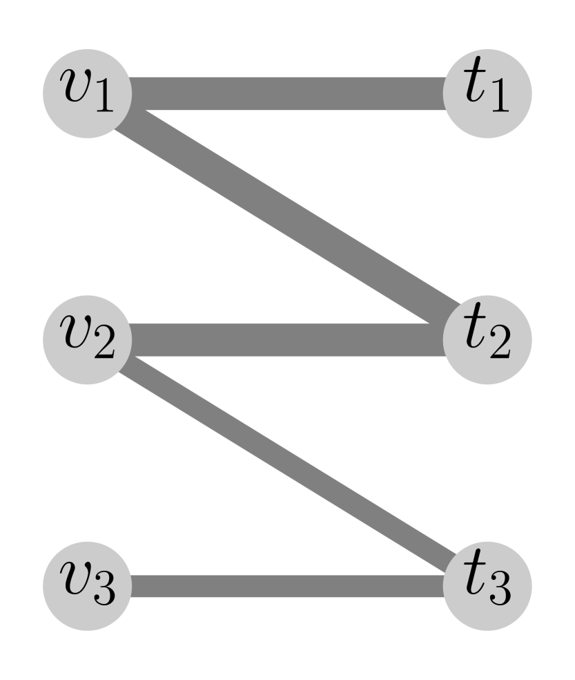
(a) $\mathrm{\theta}$ values

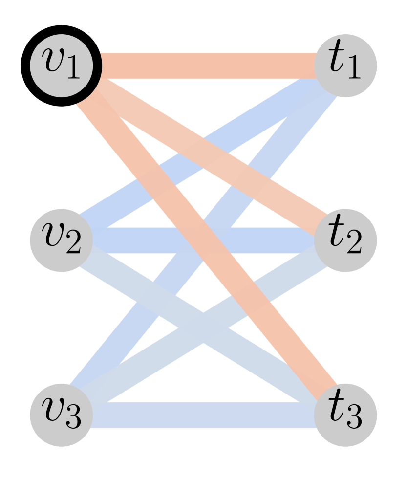
(b) Result of $v_{1}$

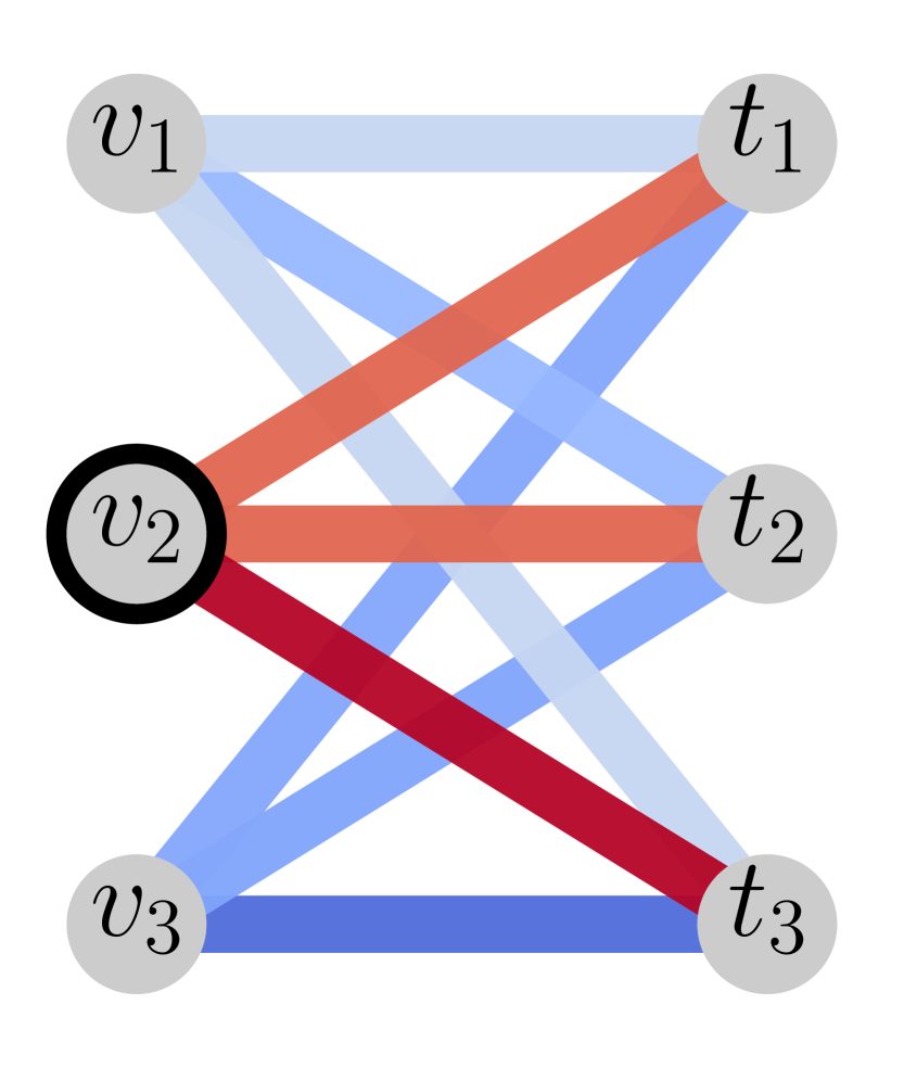
(c) Result of $v_{2}$

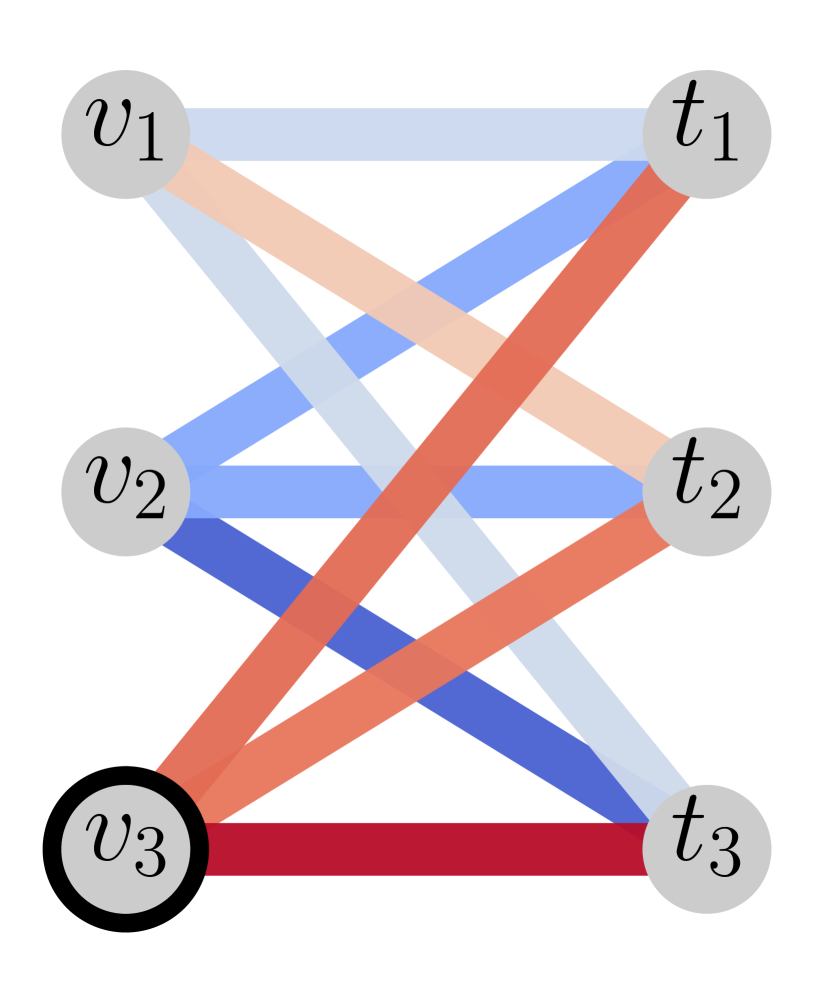
(d) Result of $v_{3}$

(e)

Figure 1: (a): Given $\mathrm{\theta}$ values. Thick and thin edges have link probabilities $0.4$ and $0.2$, respectively. (b) to (d): Sensitivity analysis results. Edge colors in (b), (c), and (d) indicate how the increase in the corresponding $\mathrm{\theta}$ entries can affect the probability of choosing $v_{1}$, $v_{2}$, and $v_{3}$, respectively.

5.1 Sensitivity analysis

We perform sensitivity analysis with a synthetic instance such that $V=\{v_{1},v_{2},v_{3}\}$, $T=\{t_{1},t_{2},t_{3}\}$, and $K=2$. Let $\theta_{i,j}$ denote the link probability of $(v_{i},t_{j})$; we set $(\theta_{1,1},\theta_{1,2},\theta_{1,3})=(0.4,0.4,0)$, $(\theta_{2,1},\theta_{2,2},\theta_{2,3})=(0,0.4,0.2)$, and $(\theta_{3,1},\theta_{3,2},\theta_{3,3})=(0,0,0.2)$ as in Figure 1. We analyze the sensitivity of Smoothed Greedy by estimating $\nabla_{\text{{\boldmath$\mathrm{\theta}$}}}\mathbb{E}_{S\sim p({\text{{\boldmath$\mathrm{\theta}$}}})}[\mbox{\boldmath$1$}_{S}]$ as explained in Section 4.1. We let $N=100$ and reduce the variance with the baseline correction method explained in Section 3.

Figures 1, 1, and 1 illustrate how and how much the increase in each $\theta_{i,j}$ value can affect the probability of choosing $v_{1}$, $v_{2}$, and $v_{3}$, respectively. In this setting, the objective values of the three maximal solutions, $\{v_{1},v_{2}\}$, $\{v_{1},v_{3}\}$, and $\{v_{2},v_{3}\}$, are $1.24$, $1.00$, and $0.76$, respectively. Therefore, Smoothed Greedy returns $\{v_{1},v_{2}\}$ or $\{v_{1},v_{3}\}$ with a high probability; this remains true even if the $\mathrm{\theta}$ values slightly change. Thus, the probability of choosing $v_{1}$ is relatively insensitive as in Figure 1. In contrast, as in Figures 1 and 1, the probabilities of choosing $v_{2}$ and $v_{3}$, respectively, are highly sensitive. For example, if $\theta_{2,3}$ increases, the probability that the algorithm returns $\{v_{1},v_{2}\}$ ($\{v_{1},v_{3}\}$) increases (decreases), which means the probability of choosing $v_{2}$ ($v_{3}$) is positively (negatively) affected by the increase in $\theta_{2,3}$. We can also see the that the opposite occurs if $\theta_{3,3}$ increases.

5.2 Decision-focused learning

Table 1: Function values achieved with each method.

	$K=5$		$K=10$		$K=20$
	Training	Test	Training	Test	Training	Test
SG-$1$	$26.3\pm 4.0$	$26.4\pm 4.4$	$46.0\pm 5.9$	$45.9\pm 6.5$	$69.7\pm 23.8$	$69.6\pm 24.1$
SG-$10$	$29.0\pm 3.7$	$28.1\pm 4.9$	$47.0\pm 12.1$	$46.1\pm 12.4$	$71.5\pm 28.0$	$70.6\pm 28.1$
SG-$100$	$33.6\pm 2.4$	$32.0\pm 3.8$	$54.3\pm 2.0$	$53.5\pm 4.2$	$82.6\pm 21.8$	$82.3\pm 21.7$
VR-SG-$10$	$35.2\pm 6.1$	$33.7\pm 6.2$	$57.9\pm 1.6$	$56.2\pm 3.4$	$90.8\pm 16.5$	$89.5\pm 16.7$
VR-SG-$100$	$\bf 36.8\pm 0.9$	$\bf 35.6\pm 2.2$	$\bf 59.9\pm 1.6$	$\bf 58.0\pm 2.9$	$\bf 96.8\pm 1.1$	$\bf 94.5\pm 2.6$
Continuous	$24.0\pm 4.5$	$23.2\pm 4.9$	$43.2\pm 6.1$	$42.3\pm 7.1$	$81.7\pm 6.8$	$81.3\pm 6.6$
Two-stage	$17.3\pm 1.2$	$17.3\pm 2.1$	$35.6\pm 0.9$	$35.6\pm 2.7$	$65.5\pm 4.0$	$64.8\pm 5.1$
Random	$17.5\pm 1.0$	$17.6\pm 2.2$	$33.8\pm 0.8$	$34.0\pm 2.7$	$64.0\pm 1.3$	$64.5\pm 2.6$

We evaluate the performance of our method via decision-focused learning experiments with MovieLens $100$K dataset [28], which contains $100,000$ ratings ($1$ to $5$) of $1,682$ movies made by $943$ users. We set the link probabilities at $0.02,0.04,\dots,0.1$ according to the ratings; those of unrated ones are set at $0$. We randomly sample $100$ movies and $500$ users, which form item set $V$ and target set $T$, respectively. We thus make $100$ random $(V,T)$ pairs with link probabilities. Each movie $v\in V$ belongs to some of $19$ genres, e.g., action and horror; we use the $19$-dimensional indicator vector as a movie feature. Each user $t\in T$ has information of their age, sex, and occupation categorized into $21$ types, e.g., writer and doctor; we concatenate them and use the resulting $24$-dimensional vector as a user feature. A feature of each $(v,t)\in V\times T$ is a concatenation of the $19$- and $24$-dimensional vectors. As a result, each of the $100$ random $(V,T)$ pairs has feature $\mathrm{X}$ of form $100\times 500\times 43$. The predictive model, which outputs $\theta_{v,t}\in[0,1]$ for the feature of each $(v,t)\in V\times T$, is a $2$-layer NN with a hidden layer of size $200$ and ReLU activation functions; the outputs are clipped to $[0,1]$. Since the features are sparse, the predictive model with default weight initialization returns $0$ too frequently; to avoid this, we set initial linear-layer weights at random non-negative values drawn from $[0,0.01]$.

We split the $100$ random instances into $80$ training and $20$ test instances; we train the predictive model with $({\text{{\boldmath$\mathrm{X}$}}}_{1},{\text{{\boldmath$\mathrm{\theta}$}}}_{1}),\dots,({\text{{\boldmath$\mathrm{X}$}}}_{80},{\text{{\boldmath$\mathrm{\theta}$}}}_{80})$ and test the performance with $(\hat{\text{{\boldmath$\mathrm{X}$}}}_{1},\hat{\text{{\boldmath$\mathrm{\theta}$}}}_{1}),\dots,(\hat{\text{{\boldmath$\mathrm{X}$}}}_{20},\hat{\text{{\boldmath$\mathrm{\theta}$}}}_{20})$. We make $30$ random training/test splits, and we present all results with means and standard deviations over the $30$ random splits. Given $80$ training datasets, we train the model over mini-batches of size $20$ for $5$ epochs. We use Adam with learning rate $10^{-3}$ for updating the model parameter, $\mathrm{w}$.

We compare SG-$N$, VR-SG-$N$, Continuous, Two-stage, and Random. SG-$N$ is our method based on Smoothed Greedy (see, Section 4.2), where $N$ indicates the number of output samples; we let $N=1$, $10$, and $100$. VR-SG-$N$ (variance-reduced SG-$N$) uses the baseline correction method when estimating gradients; we let $N=10$ and $100$ (omit $N=1$) since if $N=1$, the baseline value is equal to the single output value, which always yields zero gradients. Both SG-$N$ and VR-SG-$N$ use the greedy algorithm when making decisions. Continuous [57] maximizes the continuous relaxation of the objective function with SGA and differentiates local optima; we use their original implementation. Two-stage trains the model by minimizing the mean square error, and then maximizes the objective function with SGA; the implementation is based on that of [57]. Continuous and Two-stage make decisions $S\in\mathcal{I}$ by choosing elements corresponding to the top-$K$ entries of solution ${\text{{\boldmath$\mathrm{x}$}}}\in[0,1]^{n}$ returned by SGA. Random is a baseline method that makes uniformly random decisions $S\in\mathcal{I}$.

Table 1 shows the objective function values (averaged over the $80$ training and $20$ test instances) achieved by each method for $K=5$, $10$, and $20$. VR-SG-$100$ achieves the highest objective value for every case, and (VR-)SG with other settings also performs comparably to or better than Continuous. These results are consistent with the theoretical guarantees. More precisely, while Continuous trains the predictive model so that SGA, a $1/2$-approximation algorithm, returns high objective values, our methods train the model so that the (almost) ($1-1/\mathrm{e}$)-approximation (smoothed) greedy algorithm can achieve high objective values. We can also see that the variance reduction method is effective for improving the performance of our method. The standard deviation of (VR-)SG becomes sometimes high; this is because they are sometimes trapped in poor local optima and result in highly deviated objective values. Considering this, the performance of our method would be further improved if we can combine it with NN training techniques for escaping from poor local optima. Regarding running times, for updating $\mathrm{w}$ once, SG-$1$ takes $2.81$, $3.38$, and $3.77$ seconds on average for $K=5$, $10$, and $20$, respectively, while Continuous takes $5.86$, $5.87$, and $6.11$ seconds, respectively. Hence, our methods can run faster by performing Smoothed Greedy in parallel as mentioned in Section 4.2.

Broader Impact

The greedy algorithm for submodular maximization is one of the most extensively studied subjects of combinatorial optimization in the machine learning (ML) community. On the other hand, many recent advances in ML methods are based on continuous optimization; particularly, NNs are usually trained with stochastic first-order methods. Our work, which serves as a bridge between the combinatorial greedy algorithm and continuous first-order methods, will benefit researchers in the optimization and ML communities and practitioners who have ML tasks related to submodular maximization. Below we present examples of practical situations where our framework is useful.

• Submodular maximization sometimes appears when making vital decisions; e.g., allocation of large resources to advertising channels. In such situations, after computing a solution with the greedy algorithm, we can use our sensitivity analysis method (see, Sections 4.1 and 5.1) for assessing the reliability of the solution, i.e., how robust it is against uncertainties in parameters of objective functions. If the entries of the estimated Jacobian corresponding to the solution are small enough in absolute value, then the solution is reliable and thus we can put it into practice; otherwise, we can try using robust submodular maximization methods (e.g., [50]) to strike a balance between the objective value and reliability.

• ML tasks related to submodular maximization often involve prediction of parameters; for example, when designing diverse-recommendation systems, we need to predict users’ preferences, which correspond to the parameters. In such situations, the decision-focused learning method based on our framework (Sections 4.2 and 5.2) is useful, particularly when we do not have enough prior knowledge on how to design good predictive models and loss functions. Note that the simplicity of our method, which does not use the multilinear extension unlike [58], is also beneficial to practitioners.

As a negative aspect, failures of systems that utilize our method may result in harmful consequences. In particular, when our method is combined with NNs, how to avoid poor local optima is a practically important issue as mentioned in Section 5.2. To resolve this, we need to study the structures of objective functions that appear in each situation in detail, which we leave for future work.

Appendix A Comparisons with existing greedy methods

We present detailed comparisons of our work and the exiting studies [52, 46] on the differentiable greedy methods, which use $\operatorname*{softmax}$ instead of $\operatorname*{argmax}$. As explained below, the existing methods are devoted to differentiating some functions defined with subsets $X_{1},X_{2},\ldots\subseteq V$ given as training data. In contrast, we do not assume such subsets to be given and consider differentiating the expected value of any output-dependent quantities, $\mathbb{E}_{S\sim p({\text{{\boldmath$\mathrm{\theta}$}}})}[Q(S)]$; note that this design of our framework is the key to dealing with sensitivity analysis and decision-focused learning. Our framework can also provide more reasonable approaches to their problem settings as described below.

Tschiatschek et al. [52] consider differentiating the likelihood function, which quantifies how close an output of their algorithm can be to some good solutions, $X_{1},X_{2},\dots$, given as training data. To this end, we need to differentiate $P(X)\coloneqq\Sigma_{\sigma\in\Sigma(X)}P(\sigma,{\text{{\boldmath$\mathrm{\theta}$}}})$, where $X\in\{X_{1},X_{2},\dots\}$ is a given subset, $\Sigma(X)$ is the set of all permutations of elements in $X$, and $P(\sigma,{\text{{\boldmath$\mathrm{\theta}$}}})$ is the probability that their algorithm returns sequence $\sigma\in\mathscr{S}_{\leq K}$. Since the computation of the summation over $\Sigma(X)$ is too costly, they employ the following heuristic approximation: if the temperature of $\operatorname*{softmax}$ is low, we let $P(X)\approx P(\sigma^{G},{\text{{\boldmath$\mathrm{\theta}$}}})$, where $\sigma^{G}$ is obtained by the greedy algorithm, and if the temperature is high, we let $P(X)\approx|X|!\times P(\sigma^{R},{\text{{\boldmath$\mathrm{\theta}$}}})$, where $\sigma^{R}$ is a random permutation. As a result, the computed derivative has no theoretical guarantees unlike our gradient estimator, which is guaranteed to be unbiased. Note that with our method, we can compute an unbiased estimator of the desired derivative as follows: we let $Q(S)$ return $1$ if $S$ and $X$ consist of the same elements and $0$ otherwise, and we estimate $\nabla_{\text{{\boldmath$\mathrm{\theta}$}}}P(X)=\nabla_{\text{{\boldmath$\mathrm{\theta}$}}}\mathbb{E}_{S\sim p({\text{{\boldmath$\mathrm{\theta}$}}})}[Q(S)]$ as explained in Section 3.

Powers et al. [46] focus on some cases where we can compute derivatives more easily. They consider some loss function $L(X,{\text{{\boldmath$\mathrm{p}$}}}_{1}({\text{{\boldmath$\mathrm{\theta}$}}}),\dots,{\text{{\boldmath$\mathrm{p}$}}}_{K}({\text{{\boldmath$\mathrm{\theta}$}}}))$ that is differentiable w.r.t. ${\text{{\boldmath$\mathrm{p}$}}}_{1}({\text{{\boldmath$\mathrm{\theta}$}}}),\dots,{\text{{\boldmath$\mathrm{p}$}}}_{K}({\text{{\boldmath$\mathrm{\theta}$}}})$, where $X$ is given as training data. In their setting, ${\text{{\boldmath$\mathrm{p}$}}}_{i}({\text{{\boldmath$\mathrm{\theta}$}}})$ is given by $\operatorname*{softmax}$ and $f(X,{\text{{\boldmath$\mathrm{\theta}$}}})$ is differentiable w.r.t. $\mathrm{\theta}$. Thus, once $X$ is fixed, $\nabla_{\text{{\boldmath$\mathrm{\theta}$}}}L(X,{\text{{\boldmath$\mathrm{p}$}}}_{1}({\text{{\boldmath$\mathrm{\theta}$}}}),\dots,{\text{{\boldmath$\mathrm{p}$}}}_{K}({\text{{\boldmath$\mathrm{\theta}$}}}))$ can be readily computed via automatic differentiation. From the perspective of our method, we can regard their method as the one dealing with the case of $N=1$. More precisely, if we take $X$ to be a single output of Smoothed Greedy and let $L(X,{\text{{\boldmath$\mathrm{p}$}}}_{1}({\text{{\boldmath$\mathrm{\theta}$}}}),\dots,{\text{{\boldmath$\mathrm{p}$}}}_{K}({\text{{\boldmath$\mathrm{\theta}$}}}))=Q(X)\ln p(X,{\text{{\boldmath$\mathrm{\theta}$}}})$, then the derivative computed by their method coincides with the one obtained by using our method with $N=1$. Note that the above design of $L(\cdot)$, which is the key to obtaining unbiased gradient estimators, and the case of $N>1$ are not studied in [46]. Furthermore, if we apply our framework to their problem setting, we can use (non-differentiable) loss functions, $L(X,S)$, that measure the distance between given $X$ and output $S$ (e.g., Hamming and Levenshtein distances); we let $Q(S)=L(X,S)$ and estimate $\nabla_{\text{{\boldmath$\mathrm{\theta}$}}}\mathbb{E}_{S\sim p({\text{{\boldmath$\mathrm{\theta}$}}})}[L(X,S)]$.

Appendix B Proofs of approximation guarantees

In the following discussion, $S_{k}$ denotes the solution constructed in the $k$-th step of Algorithm 1; we let $S_{0}=\emptyset$. For simplicity, we omit the fixed parameter, $\mathrm{\theta}$, in the proofs.

See 1

Proof.

From the rule of choosing $s_{k}$, we have $\mathbb{E}[f_{{S}}({s_{k}})]=\left\langle{{\text{{\boldmath$\mathrm{g}$}}}_{k},{\text{{\boldmath$\mathrm{p}$}}}_{k}}\right\rangle$. Let $\mbox{\boldmath$1$}_{u}\in\mathbb{R}^{n_{k}}$ be the indicator vector of $u\in{U_{k}}$. Since $\left\langle{{\text{{\boldmath$\mathrm{g}$}}}_{k},\mbox{\boldmath$1$}_{u}}\right\rangle=f_{{S}}({u})$ and $\mbox{\boldmath$1$}_{u}\in\Delta^{n_{k}}$ hold, we can obtain the lemma as follows:

$$\mathbb{E}[f_{{S}}({s_{k}})]=\left\langle{{\text{{\boldmath$\mathrm{g}$}}}_{k},{\text{{\boldmath$\mathrm{p}$}}}_{k}}\right\rangle =\max_{{\text{{\boldmath$\mathrm{p}$}}}\in\Delta^{n_{k}}}\{\left\langle{{\text{{\boldmath$\mathrm{g}$}}}_{k},{\text{{\boldmath$\mathrm{p}$}}}}\right\rangle-\Omega_{k}({\text{{\boldmath$\mathrm{p}$}}})\}+\Omega_{k}({\text{{\boldmath$\mathrm{p}$}}}_{k})$$ (A1)

$$\geq\left\langle{{\text{{\boldmath$\mathrm{g}$}}}_{k},\mbox{\boldmath$1$}_{u}}\right\rangle-(\Omega_{k}(\mbox{\boldmath$1$}_{u})-\Omega_{k}({\text{{\boldmath$\mathrm{p}$}}}_{k}))\geq f_{{S}}({u})-\delta,$$ (A2)

where the last inequality comes from $\delta\geq\Omega_{k}({\text{{\boldmath$\mathrm{p}$}}})-\Omega_{k}({\text{{\boldmath$\mathrm{q}$}}})$ for any ${\text{{\boldmath$\mathrm{p}$}}},{\text{{\boldmath$\mathrm{q}$}}}\in\Delta^{{n_{k}}}$. ∎

See 1

Proof.

Fix $k\in\{1,\dots,K\}$ arbitrarily and take all random quantities to be conditioned on the ($k-1$)-th step. From 1 with $O\backslash S_{k-1}\subseteq{U_{k}}$ and the submodularity, we obtain

$$\mathbb{E}[f_{{S_{k-1}}}({s_{k}})]\geq\frac{1}{K}\sum_{v\in O\backslash S_{k-1}}f_{{S_{k-1}}}({v})-\delta\geq\frac{1}{K}f_{{S_{k-1}}}({O})-\delta.$$

By taking expectation over all possible realizations of the ($k-1$)-th step and using the monotonicity, we obtain

$$\mathbb{E}[f(S_{k})]-\mathbb{E}[f(S_{k-1})]\geq\frac{1}{K}(\mathbb{E}[f(O\cup S_{k-1})]-\mathbb{E}[f(S_{k-1})])-\delta\geq\frac{1}{K}(f(O)-\mathbb{E}[f(S_{k-1})])-\delta.$$

Therefore, as is often the case with the analysis of the greedy algorithm, we can obtain the following inequality by induction:

$$\mathbb{E}[f(S_{K})]\geq\left(1-\left(1-\frac{1}{K}\right)^{K}\right)f(O)-\delta\sum_{k=0}^{K-1}\left(1-\frac{1}{K}\right)^{k}\geq\left(1-\frac{1}{\mathrm{e}}\right)f(O)-\delta K,$$

where we used $f(\emptyset)=0$. Hence we obtain the theorem from $\mathbb{E}[f(S)]=\mathbb{E}[f(S_{K})]$. ∎

See 2

Proof.

For each realization of $S_{0}\subset S_{1}\subset\dots\subset S_{|S|}=S\in\mathcal{I}$, we define $S_{{|S|}+1},S_{{|S|}+2},\dots,S_{K}$ as $S$. We thus construct a series of feasible solutions, $S_{0},S_{1},\dots,S_{K}$, for every realization. Note that $\mathbb{E}[f(S)]=\mathbb{E}[f(S_{K})]$ holds since we always have $S=S_{K}$.

We consider constructing a series of subsets $O_{0},O_{1},\dots,O_{K}$ for each realization of $S_{0},S_{1},\dots,S_{K}$. We aim to prove that we can construct such $O_{0},O_{1},\dots,O_{K}$ satisfying the following conditions: $O_{0}=O$, $S_{i}\subseteq O_{i}\in\mathcal{I}$ ($i=0,\dots,K-1$), $S_{K}=O_{K}\in\mathcal{I}$ for every realization, and

$$\kappa\cdot(\mathbb{E}[f(S_{i})]-\mathbb{E}[f(S_{i-1})]+\delta)\geq\mathbb{E}[f(O_{i-1})]-\mathbb{E}[f(O_{i})]$$ (A3)

for $i=1,\dots,K$.

In the case of $i=0$, we let $O_{0}=O$, which satisfies $S_{0}=\emptyset\subseteq O=O_{0}\in\mathcal{I}$. In this case, (A3) is not required to hold.

We assume all random quantities to be conditioned on an arbitrary realization of the ($k-1$)-th step, where $S_{0},\dots,S_{k-1}$ and $O_{0},\dots,O_{k-1}$ satisfying $S_{i}\subseteq O_{i}\in\mathcal{I}$ ($i=0,\dots,k-1$) are given. If $S_{k-1}$ is maximal, we let $O_{k}=S_{k}$ ($=S_{k-1}=O_{k-1}$), which satisfies $S_{k}=O_{k}\in\mathcal{I}$ and

$$\kappa\cdot(\mathbb{E}[f(S_{k})]-f(S_{k-1})+\delta)=\kappa\cdot\delta\geq 0=f(O_{k-1})-\mathbb{E}[f(O_{k})].$$

If $S_{k-1}$ is not maximal, from the definition of $\kappa$-extensible systems, for any choice of $s_{k}\notin S_{k-1}$, there exists $Z_{k}\subseteq O_{k-1}\backslash S_{k-1}$ such that $O_{k-1}\backslash Z_{k}\cup\{s_{k}\}\in\mathcal{I}$ and $|Z_{k}|\leq\kappa$ hold. We let $O_{k}=O_{k-1}\backslash Z_{k}\cup\{s_{k}\}$. Note that thus constructed $O_{k}$ satisfies $S_{k}\subseteq O_{k}\in\mathcal{I}$ for any realization of the $k$-th step; moreover, if $k=K$, we always have $S_{K}=O_{K}\in\mathcal{I}$ since $S_{K}$ is maximal in any realization. Considering expectation over realizations of the $k$-th step, we obtain

$$f(O_{k-1})-\mathbb{E}[f(O_{k})]$$ (A4)

$$={} f(O_{k-1})-\mathbb{E}[f(O_{k-1}\backslash Z_{k})]$$ (A5)

$$\qquad\quad\ \ \,+\mathbb{E}[f(O_{k-1}\backslash Z_{k})]-\mathbb{E}[f(O_{k})]$$ (A6)

$$\leq{} \mathbb{E}[f_{{O_{k-1}\backslash Z_{k}}}({Z_{k}})] \because\text{$O_{k-1}\backslash Z_{k}\subseteq O_{k}$ and monotonicity}$$ (A7)

$$\leq{} \mathbb{E}\left[\sum_{v\in Z_{k}}f_{{S_{k-1}}}({v})\right] \because\text{$S_{k-1}\subseteq O_{k-1}\backslash Z_{k}$ and submodularity}$$ (A8)

$$\leq{} \kappa\cdot(\mathbb{E}[f_{{S_{k-1}}}({s_{k}})]+\delta) \because\text{$Z_{k}\subseteq O_{k-1}\backslash S_{k-1}\subseteq{U_{k}}$, \lx@cref{creftypecap~refnum}{lem:fdel}, and $|Z_{k}|\leq\kappa$}$$ (A9)

$$={} \kappa\cdot(\mathbb{E}[f(S_{k})]-f(S_{k-1})+\delta)$$ (A10)

Therefore, in any case we have

$$\kappa\cdot(\mathbb{E}[f(S_{k})]-f(S_{k-1})+\delta)\geq f(O_{k-1})-\mathbb{E}[f(O_{k})].$$

By taking expectation over all realizations of the ($k-1$)-th step, we obtain (A3) for $i=k$. For every realization, $O_{0},\dots,O_{k}$ constructed above satisfy $S_{i}\subseteq O_{i}\in\mathcal{I}$ for $i=0,\dots,k$ (if $k=K$, we have $S_{k}=O_{k}\in\mathcal{I}$). This means that the assumption of induction for the next step is satisfied. Consequently, (A3) holds for $i=1,\dots,K$ by induction. Summing both sides of (A3) for $i=1,\dots,K$, we obtain

$$\kappa\cdot(\mathbb{E}[f(S_{K})]-f(\emptyset)+\delta K)\geq\mathbb{E}[f(O_{0})]-\mathbb{E}[f(O_{K})].$$

Since we have $f(\emptyset)=0$, $O_{0}=O$, and $O_{K}=S_{K}$ for every realization, it holds that

$$\mathbb{E}[f(S_{K})]\geq\frac{1}{\kappa+1}f(O)-\frac{\kappa}{\kappa+1}\delta K\geq\frac{1}{\kappa+1}f(O)-\delta K.$$

Hence we obtain the theorem from $\mathbb{E}[f(S)]=\mathbb{E}[f(S_{K})]$. ∎

Appendix C Regularization functions

We first detail the case where $\Omega_{k}$ is the entropy function. We then present a sufficient condition for satisfying 2, which is useful when designing regularization functions.

C.1 Entropy regularization

We consider using the entropy function as a regularization function: $\Omega_{k}({\text{{\boldmath$\mathrm{p}$}}})=\epsilon\sum_{u\in{U_{k}}}p(u)\ln p(u)$, where $\epsilon>0$ is a constant that controls the perturbation strength. Note that we have $\Omega_{k}({\text{{\boldmath$\mathrm{p}$}}})-\Omega_{k}({\text{{\boldmath$\mathrm{q}$}}})\leq\epsilon\cdot 0-\epsilon\sum_{i=1}^{n_{k}}\frac{1}{{n_{k}}}\ln\frac{1}{{n_{k}}}=\epsilon\ln{n_{k}}$ for any ${\text{{\boldmath$\mathrm{p}$}}},{\text{{\boldmath$\mathrm{q}$}}}\in\Delta^{n_{k}}$.

From the relationship between the entropy regularization and $\operatorname*{softmax}$, each iteration of Smoothed Greedy can be performed via softmax sampling. More precisely, from the Karush–Kuhn–Tucker (KKT) condition of problem (2), $\max_{{\text{{\boldmath$\mathrm{p}$}}}\in\Delta^{{n_{k}}}}\{\left\langle{{\text{{\boldmath$\mathrm{g}$}}}_{k},{\text{{\boldmath$\mathrm{p}$}}}}\right\rangle-\Omega_{k}({\text{{\boldmath$\mathrm{p}$}}})\}$, we have

$$\epsilon(\ln{\text{{\boldmath$\mathrm{p}$}}}+\mbox{\boldmath$1$}_{n_{k}})-{\text{{\boldmath$\mathrm{g}$}}}_{k}+\mbox{\boldmath$1$}_{n_{k}}\mu=\mbox{\boldmath$0$}_{n_{k}}\quad\text{and}\quad\mbox{\boldmath$1$}_{n_{k}}^{\top}{\text{{\boldmath$\mathrm{p}$}}}=1,$$ (A11)

where $\ln$ operates in an element-wise manner and $\mu\in\mathbb{R}$ is a multiplier corresponding to the equality constraint. Note that we need not take the inequality constraints, ${\text{{\boldmath$\mathrm{p}$}}}\geq\mbox{\boldmath$0$}_{n_{k}}$, into account since the entropy regularization forces every $p(u)$ to be positive. Since $\Omega_{k}$ is strictly convex and every feasible solution satisfies the linear independence constraint qualification (LICQ), the maximizer, ${\text{{\boldmath$\mathrm{p}$}}}_{k}$, is characterized as the unique solution to the KKT equation system (A11). From (A11), we see that ${\text{{\boldmath$\mathrm{p}$}}}_{k}$ is proportional to $\exp({\text{{\boldmath$\mathrm{g}$}}}_{k}/\epsilon)$. Thus, Steps 4 to 6 in Algorithm 1 can be performed via softmax sampling: $p_{k}(u,{\text{{\boldmath$\mathrm{\theta}$}}})\propto\exp(f_{{S_{k-1}}}({u},{{\text{{\boldmath$\mathrm{\theta}$}}}})/\epsilon)$ for $u\in{U_{k}}$, which takes $\mathrm{O}({n_{k}})$ time if $f_{{S_{k-1}}}({u},{{\text{{\boldmath$\mathrm{\theta}$}}}})$ values are given.

We then discuss how to compute $\nabla_{{\text{{\boldmath$\mathrm{g}$}}}_{k}}{\text{{\boldmath$\mathrm{p}$}}}_{k}({\text{{\boldmath$\mathrm{g}$}}}_{k})$. While this can be done by directly differentiating $p_{k}(u,{\text{{\boldmath$\mathrm{g}$}}}_{k})\propto\exp(g_{k}(u)/\epsilon)$, we here see how to compute it by applying the implicit function theorem (see, e.g., [16]) to the KKT equation system (A11) as a warm-up for the next section. In this case, the requirements for using the implicit function theorem are satisfied (see the next section). By differentiating the KKT equation system (A11) w.r.t. ${\text{{\boldmath$\mathrm{g}$}}}_{k}$, we obtain

$$\begin{bmatrix}\epsilon\mathrm{diag}({\text{{\boldmath$\mathrm{p}$}}}_{k})^{-1}&\mbox{\boldmath$1$}_{n_{k}}\\ \mbox{\boldmath$1$}_{n_{k}}^{\top}&0\end{bmatrix}\begin{bmatrix}\nabla_{{\text{{\boldmath$\mathrm{g}$}}}_{k}}{\text{{\boldmath$\mathrm{p}$}}}_{k}\\ \nabla_{{\text{{\boldmath$\mathrm{g}$}}}_{k}}\mu\end{bmatrix}=\begin{bmatrix}{\text{{\boldmath$\mathrm{I}$}}}_{n_{k}}\\ \mbox{\boldmath$0$}_{n_{k}}^{\top}\end{bmatrix},$$ (A12)

where $\mathrm{diag}({\text{{\boldmath$\mathrm{p}$}}}_{k})$ is a diagonal matrix whose diagonal entries are ${\text{{\boldmath$\mathrm{p}$}}}_{k}$ and ${\text{{\boldmath$\mathrm{I}$}}}_{n_{k}}$ is the ${n_{k}}\times{n_{k}}$ identity matrix. We can compute $\nabla_{{\text{{\boldmath$\mathrm{g}$}}}_{k}}{\text{{\boldmath$\mathrm{p}$}}}_{k}$ by solving the above equation as follows:

$$\begin{bmatrix}\nabla_{{\text{{\boldmath$\mathrm{g}$}}}_{k}}{\text{{\boldmath$\mathrm{p}$}}}_{k}\\ \nabla_{{\text{{\boldmath$\mathrm{g}$}}}_{k}}\mu\end{bmatrix}=\begin{bmatrix}\epsilon\mathrm{diag}({\text{{\boldmath$\mathrm{p}$}}}_{k})^{-1}&\mbox{\boldmath$1$}_{n_{k}}\\ \mbox{\boldmath$1$}_{n_{k}}^{\top}&0\end{bmatrix}^{-1}\begin{bmatrix}{\text{{\boldmath$\mathrm{I}$}}}_{n_{k}}\\ \mbox{\boldmath$0$}_{n_{k}}^{\top}\end{bmatrix}=\begin{bmatrix}\epsilon^{-1}(\mathrm{diag}({\text{{\boldmath$\mathrm{p}$}}}_{k})-{\text{{\boldmath$\mathrm{p}$}}}_{k}{\text{{\boldmath$\mathrm{p}$}}}_{k}^{\top})\\ {\text{{\boldmath$\mathrm{p}$}}}_{k}^{\top}\end{bmatrix}.$$ (A13)

Note that once we obtain $\nabla_{\text{{\boldmath$\mathrm{\theta}$}}}{\text{{\boldmath$\mathrm{g}$}}}_{k}({\text{{\boldmath$\mathrm{\theta}$}}})$, we can compute the desired derivative, $\nabla_{\text{{\boldmath$\mathrm{\theta}$}}}{\text{{\boldmath$\mathrm{p}$}}}_{k}({\text{{\boldmath$\mathrm{\theta}$}}})=\nabla_{{\text{{\boldmath$\mathrm{g}$}}}_{k}}{\text{{\boldmath$\mathrm{p}$}}}_{k}({\text{{\boldmath$\mathrm{g}$}}}_{k})\cdot\nabla_{\text{{\boldmath$\mathrm{\theta}$}}}{\text{{\boldmath$\mathrm{g}$}}}_{k}({\text{{\boldmath$\mathrm{\theta}$}}})=\epsilon^{-1}(\mathrm{diag}({\text{{\boldmath$\mathrm{p}$}}}_{k})-{\text{{\boldmath$\mathrm{p}$}}}_{k}{\text{{\boldmath$\mathrm{p}$}}}_{k}^{\top})\nabla_{\text{{\boldmath$\mathrm{\theta}$}}}{\text{{\boldmath$\mathrm{g}$}}}_{k}({\text{{\boldmath$\mathrm{\theta}$}}})$, by matrix-vector products in $\mathrm{O}({n_{k}}\times\dim\Theta)$ time.

One may get interested in the link between problem (2) with the entropy regularization and the optimal transport (OT) with entropy regularization [12]. Specifically, while (2) has a vector variable with one equality constraint, OT has a matrix variable with two equality constraints; in this sense, (2) considers a simpler setting. Thanks to the simplicity, we can analyze the theoretical guarantees of Smoothed Greedy. In contrast, if we consider using OT, we can employ more sophisticated operations, e.g., ranking and sorting [13], than $\operatorname*{argmax}$. In return for this, however, it becomes more difficult to prove approximation guarantees; for example, how to design transportation costs is non-trivial. This OT-based approach to designing differentiable combinatorial optimization algorithms will be an interesting research direction, which we leave for future work.

C.2 Sufficient condition for satisfying 2

We study the case where $\Omega_{k}$ is a general strictly convex differentiable function; although a similar discussion is presented in [3] for the case where $\Omega_{k}$ is quadratic, we here provide a detailed analysis with general $\Omega_{k}$ for completeness. The KKT condition of problem (2) can be written as

$$\nabla_{\text{{\boldmath$\mathrm{p}$}}}\Omega_{k}({\text{{\boldmath$\mathrm{p}$}}})-{\text{{\boldmath$\mathrm{g}$}}}_{k}-{\text{{\boldmath$\mathrm{\lambda}$}}}+\mbox{\boldmath$1$}_{n_{k}}\mu=\mbox{\boldmath$0$}_{n_{k}}, {\text{{\boldmath$\mathrm{\lambda}$}}}\odot{\text{{\boldmath$\mathrm{p}$}}}=\mbox{\boldmath$0$}_{n_{k}}, \mbox{\boldmath$1$}_{n_{k}}^{\top}{\text{{\boldmath$\mathrm{p}$}}}=1,$$ and (A14)

where ${\text{{\boldmath$\mathrm{\lambda}$}}}\geq\mbox{\boldmath$0$}_{n_{k}}$ consists of multipliers corresponding to the inequality constraints, ${\text{{\boldmath$\mathrm{p}$}}}\geq\mbox{\boldmath$0$}_{n_{k}}$, and $\odot$ denotes the element-wise product. Since every feasible point in $\Delta^{n_{k}}$ satisfies LICQ, if $\Omega_{k}$ is strictly convex on $\Delta^{n_{k}}$, the optimal solution is uniquely characterized by the KKT condition. Let $(\tilde{\text{{\boldmath$\mathrm{p}$}}},\tilde{\text{{\boldmath$\mathrm{\lambda}$}}},\tilde{\mu})$ be a triplet that satisfies the KKT condition, where $\tilde{{\text{{\boldmath$\mathrm{p}$}}}}={\text{{\boldmath$\mathrm{p}$}}}_{k}$. If the following three conditions hold, $\nabla_{{\text{{\boldmath$\mathrm{g}$}}}_{k}}{\text{{\boldmath$\mathrm{p}$}}}_{k}$ can be calculated from the KKT condition as detailed later:

1. $\Omega_{k}$ is twice-differentiable,

2. the Hessian, $\nabla_{\text{{\boldmath$\mathrm{p}$}}}^{2}\Omega_{k}({\text{{\boldmath$\mathrm{p}$}}})$, is positive definite for any ${\text{{\boldmath$\mathrm{p}$}}}\in\Delta^{n_{k}}$, and

3. the strict complementarity, $\tilde{\text{{\boldmath$\mathrm{\lambda}$}}}+\tilde{\text{{\boldmath$\mathrm{p}$}}}>\mbox{\boldmath$0$}_{n_{k}}$, holds at the unique optimum, $\tilde{\text{{\boldmath$\mathrm{p}$}}}={\text{{\boldmath$\mathrm{p}$}}}_{k}$.

Note that the second condition implies the strict convexity of $\Omega_{k}$ on $\Delta^{{n_{k}}}$. Therefore, a sufficient condition for satisfying 2 is given by the above three conditions. In practice, given any twice-differentiable convex function, we can add to it the entropy function multiplied by a small constant for obtaining $\Omega_{k}$ that satisfies the sufficient condition.

We then explain how to compute $\nabla_{{\text{{\boldmath$\mathrm{g}$}}}_{k}}{\text{{\boldmath$\mathrm{p}$}}}_{k}$. Let ${\tilde{U}}$ be a subset of ${U_{k}}$ such that $\tilde{p}(u)=0$ iff $u\in{\tilde{U}}$; the strict complementarity implies $\tilde{\lambda}(u)=0$ iff $u\notin{\tilde{U}}$. We let ${\text{{\boldmath$\mathrm{x}$}}}\coloneqq({\text{{\boldmath$\mathrm{p}$}}},{\text{{\boldmath$\mathrm{\lambda}$}}}_{\tilde{U}},\mu)$, where ${\text{{\boldmath$\mathrm{\lambda}$}}}_{\tilde{U}}$ is a $|{\tilde{U}}|$-dimensional vector consisting of the entries of $\mathrm{\lambda}$ corresponding to ${\tilde{U}}$. We define ${\text{{\boldmath$\mathrm{I}$}}}_{\tilde{U}}$ as the ${n_{k}}\times|{\tilde{U}}|$ matrix that has columns of ${\text{{\boldmath$\mathrm{I}$}}}_{n_{k}}$ corresponding to ${\tilde{U}}$. The KKT equation system at $\tilde{{\text{{\boldmath$\mathrm{x}$}}}}=(\tilde{\text{{\boldmath$\mathrm{p}$}}},\tilde{\text{{\boldmath$\mathrm{\lambda}$}}}_{\tilde{U}},\tilde{\mu})$ can be written as

$$H({\text{{\boldmath$\mathrm{x}$}}},{\text{{\boldmath$\mathrm{g}$}}}_{k})\coloneqq\begin{bmatrix}\nabla_{\text{{\boldmath$\mathrm{p}$}}}\Omega_{k}({\text{{\boldmath$\mathrm{p}$}}})-{\text{{\boldmath$\mathrm{g}$}}}_{k}-{\text{{\boldmath$\mathrm{I}$}}}_{\tilde{U}}{\text{{\boldmath$\mathrm{\lambda}$}}}_{\tilde{U}}+\mbox{\boldmath$1$}_{n_{k}}\mu\\ -{\text{{\boldmath$\mathrm{I}$}}}_{\tilde{U}}^{\top}{\text{{\boldmath$\mathrm{p}$}}}\\ \mbox{\boldmath$1$}_{n_{k}}^{\top}{\text{{\boldmath$\mathrm{p}$}}}-1\end{bmatrix}=\begin{bmatrix}\mbox{\boldmath$0$}_{n_{k}}\\ \mbox{\boldmath$0$}_{|{\tilde{U}}|}\\ 0\end{bmatrix},$$ (A15)

and its partial Jacobians at $\tilde{{\text{{\boldmath$\mathrm{x}$}}}}$ are given by

$$\nabla_{\text{{\boldmath$\mathrm{x}$}}}H(\tilde{{\text{{\boldmath$\mathrm{x}$}}}},{\text{{\boldmath$\mathrm{g}$}}}_{k})=\begin{bmatrix}\nabla_{\text{{\boldmath$\mathrm{p}$}}}^{2}\Omega_{k}(\tilde{{\text{{\boldmath$\mathrm{p}$}}}})&-{\text{{\boldmath$\mathrm{I}$}}}_{\tilde{U}}&\mbox{\boldmath$1$}_{n_{k}}\\ -{\text{{\boldmath$\mathrm{I}$}}}_{\tilde{U}}^{\top}&\lx@intercol\hfil\hbox{\multirowsetup $\mbox{\boldmath$0$}_{|{\tilde{U}}|+1\times|{\tilde{U}}|+1}$ }\hfil\lx@intercol\\ \mbox{\boldmath$1$}_{n_{k}}^{\top}&\end{bmatrix} \nabla_{{\text{{\boldmath$\mathrm{g}$}}}_{k}}H(\tilde{{\text{{\boldmath$\mathrm{x}$}}}},{\text{{\boldmath$\mathrm{g}$}}}_{k})=\begin{bmatrix}-{\text{{\boldmath$\mathrm{I}$}}}_{n_{k}}\\ \mbox{\boldmath$0$}_{|{\tilde{U}}|\times{n_{k}}}\\ \mbox{\boldmath$0$}_{n_{k}}^{\top}\end{bmatrix}.$$ and (A16)

Note that $|{\tilde{U}}|<{n_{k}}$ always holds; otherwise $\tilde{{\text{{\boldmath$\mathrm{p}$}}}}=\mbox{\boldmath$0$}_{n_{k}}$, which is an infeasible solution. Therefore, $[-{\text{{\boldmath$\mathrm{I}$}}}_{\tilde{U}}\ \mbox{\boldmath$1$}_{n_{k}}]$ always has rank $|{\tilde{U}}|+1$. From the positive definiteness of $\nabla_{\text{{\boldmath$\mathrm{p}$}}}^{2}\Omega_{k}(\tilde{{\text{{\boldmath$\mathrm{p}$}}}})$, we have

$$\det\left(\nabla_{\text{{\boldmath$\mathrm{x}$}}}H(\tilde{{\text{{\boldmath$\mathrm{x}$}}}},{\text{{\boldmath$\mathrm{g}$}}}_{k})\right)=\det\left(\nabla_{\text{{\boldmath$\mathrm{p}$}}}^{2}\Omega_{k}(\tilde{{\text{{\boldmath$\mathrm{p}$}}}})\right)\det\left(-[-{\text{{\boldmath$\mathrm{I}$}}}_{\tilde{U}}\ \mbox{\boldmath$1$}_{n_{k}}]^{\top}\nabla_{\text{{\boldmath$\mathrm{p}$}}}^{2}\Omega_{k}(\tilde{{\text{{\boldmath$\mathrm{p}$}}}})^{-1}[-{\text{{\boldmath$\mathrm{I}$}}}_{\tilde{U}}\ \mbox{\boldmath$1$}_{n_{k}}]\right)\neq 0,$$

where we used the Schur complement. Hence $\nabla_{\text{{\boldmath$\mathrm{x}$}}}H(\tilde{{\text{{\boldmath$\mathrm{x}$}}}},{\text{{\boldmath$\mathrm{g}$}}}_{k})$ is non-singular. This guarantees that $\nabla_{{\text{{\boldmath$\mathrm{g}$}}}_{k}}{\text{{\boldmath$\mathrm{p}$}}}_{k}$ can be computed by using the implicit function theorem as follows (see, e.g., [16]):

$$\begin{bmatrix}\nabla_{{\text{{\boldmath$\mathrm{g}$}}}_{k}}{\text{{\boldmath$\mathrm{p}$}}}_{k}\\ \nabla_{{\text{{\boldmath$\mathrm{g}$}}}_{k}}\tilde{{\text{{\boldmath$\mathrm{\lambda}$}}}}_{\tilde{U}}\\ \nabla_{{\text{{\boldmath$\mathrm{g}$}}}_{k}}\tilde{\mu}\end{bmatrix}=-\nabla_{\text{{\boldmath$\mathrm{x}$}}}H(\tilde{{\text{{\boldmath$\mathrm{x}$}}}},{\text{{\boldmath$\mathrm{g}$}}}_{k})^{-1}\nabla_{{\text{{\boldmath$\mathrm{g}$}}}_{k}}H(\tilde{{\text{{\boldmath$\mathrm{x}$}}}},{\text{{\boldmath$\mathrm{g}$}}}_{k}).$$ (A17)

Thus, once the KKT triplet, the Hessian, and $\nabla_{\text{{\boldmath$\mathrm{\theta}$}}}{\text{{\boldmath$\mathrm{g}$}}}_{k}({\text{{\boldmath$\mathrm{\theta}$}}})$ are obtained, we can compute $\nabla_{\text{{\boldmath$\mathrm{\theta}$}}}{\text{{\boldmath$\mathrm{p}$}}}_{k}({\text{{\boldmath$\mathrm{\theta}$}}})=\nabla_{{\text{{\boldmath$\mathrm{g}$}}}_{k}}{\text{{\boldmath$\mathrm{p}$}}}_{k}({\text{{\boldmath$\mathrm{g}$}}}_{k})\cdot\nabla_{\text{{\boldmath$\mathrm{\theta}$}}}{\text{{\boldmath$\mathrm{g}$}}}_{k}({\text{{\boldmath$\mathrm{\theta}$}}})$ in $\mathrm{O}({n_{k}}^{3}+{n_{k}}^{2}\times\dim\Theta)$ time in general. For speeding up this step, we can reduce the ${n_{k}}$ value by using the stochastic version of the greedy algorithm [38] (see, Section F.2).

A recent result [51] provides an extended version of the implicit function theorem, which may enable us to deal with a wider class of $\Omega_{k}$; we leave this for future work.

Appendix D Discussion on other gradient estimators

The score-function gradient estimator is one of major Monte Carlo gradient estimators. Other than that, the pathwise and measure-valued gradient estimators are widely used (see, [40] for a survey). The Gumbel-Softmax estimator [30, 36] has also been used in many recent studies. We discuss why it is difficult to use those estimators for our case.

The pathwise gradient estimators basically use derivatives of quantities inside the expectation. In our case, however, we cannot differentiate the quantity, $Q(S)$, w.r.t. $S$ since the domain is non-continuous.

The measure-valued gradient estimators require us to decompose $\nabla_{\text{{\boldmath$\mathrm{\theta}$}}}p({\text{{\boldmath$\mathrm{\theta}$}}})$ into $p^{+}({\text{{\boldmath$\mathrm{\theta}$}}})$ and $p^{-}({\text{{\boldmath$\mathrm{\theta}$}}})$, which must satisfy the following conditions: both $p^{+}({\text{{\boldmath$\mathrm{\theta}$}}})$ and $p^{-}({\text{{\boldmath$\mathrm{\theta}$}}})$ form some probability distribution functions, and $\nabla_{\text{{\boldmath$\mathrm{\theta}$}}}p({\text{{\boldmath$\mathrm{\theta}$}}})=c_{\text{{\boldmath$\mathrm{\theta}$}}}(p^{+}({\text{{\boldmath$\mathrm{\theta}$}}})-p^{-}({\text{{\boldmath$\mathrm{\theta}$}}}))$ holds with some constant $c_{\text{{\boldmath$\mathrm{\theta}$}}}$. Once we obtain a decomposition satisfying these conditions, we can estimate the gradient by sampling from $p^{+}({\text{{\boldmath$\mathrm{\theta}$}}})$ and $p^{-}({\text{{\boldmath$\mathrm{\theta}$}}})$. It is known that we can obtain such a decomposition when $p({\text{{\boldmath$\mathrm{\theta}$}}})$ has certain structures, e.g., Poisson and Gaussian. In our case, however, $p({\text{{\boldmath$\mathrm{\theta}$}}})$ is the output distribution, and how to decompose it is non-trivial; in fact, this seems to be very difficult.

The Gumbel-Softmax estimator is obtained by continuously interpolating discrete categorical distributions (defined on $\Delta^{{n_{k}}}$ in our case) and computing derivatives at interior points. In our case, however, we must obtain an extreme point, $S_{k-1}$, in the ($k-1$)-th step to compute the categorical distribution ${\text{{\boldmath$\mathrm{p}$}}}_{k}({\text{{\boldmath$\mathrm{\theta}$}}})$ used in the $k$-th step. That is, unlike the cases of [30, 36], Smoothed Greedy sequentially samples from categorical distributions that depend on the past samples. Consequently, the continuous interpolation for a single step does not work for smoothing the sequential $\operatorname*{argmax}$; hence we cannot apply the Gumbel-Softmax estimator to our setting.

Appendix E Learning submodular models with limited oracle queries

We discuss the application of our framework to learning of parameterized submodular functions with limited oracle queries. We also provide experiments on learning deep submodular functions [15].

E.1 Problem description

We consider maximizing unknown submodular function $\hat{f}(\cdot)$ by sequentially querying its values. Specifically, in each $t$-th round, we can query $\hat{f}(\cdot)$ values at $N$ points $S_{1},\dots,S_{N}\in\mathcal{I}$, and by using this feedback, we seek a good solution for maximizing $\hat{f}(\cdot)$. We suppose that no prior knowledge on the true function, $\hat{f}(\cdot)$, other than the fact that it is normalized, monotone, and submodular, is available and that to query the true function value is costly and time-consuming. We want to achieve high $\hat{f}(\cdot)$ values with a small number of rounds and queries. One can think of this setting as a variant of submodular maximization with low adaptive complexities [5] or online submodular maximization with bandit feedback [60].

We consider the following approach: we construct some parameterized submodular model $f(\cdot,{\text{{\boldmath$\mathrm{\theta}$}}})$, e.g., a deep submodular function, and update $\mathrm{\theta}$ by using our gradient estimators with $Q(S_{j})=\hat{f}(S_{j})$. That is, akin to the decision-focused approach described in Section 4.2, we train $f(\cdot,{\text{{\boldmath$\mathrm{\theta}$}}})$ so that the greedy algorithm can achieve high $\hat{f}(\cdot)$ values; the current setting is more difficult since we know nothing about $\hat{f}(\cdot)$ in advance and features, which are used by the predictive models, are unavailable.

E.2 Experiments

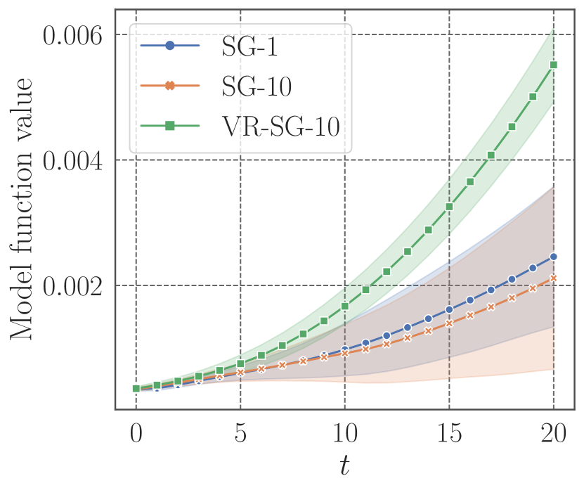
(a) Noise-free

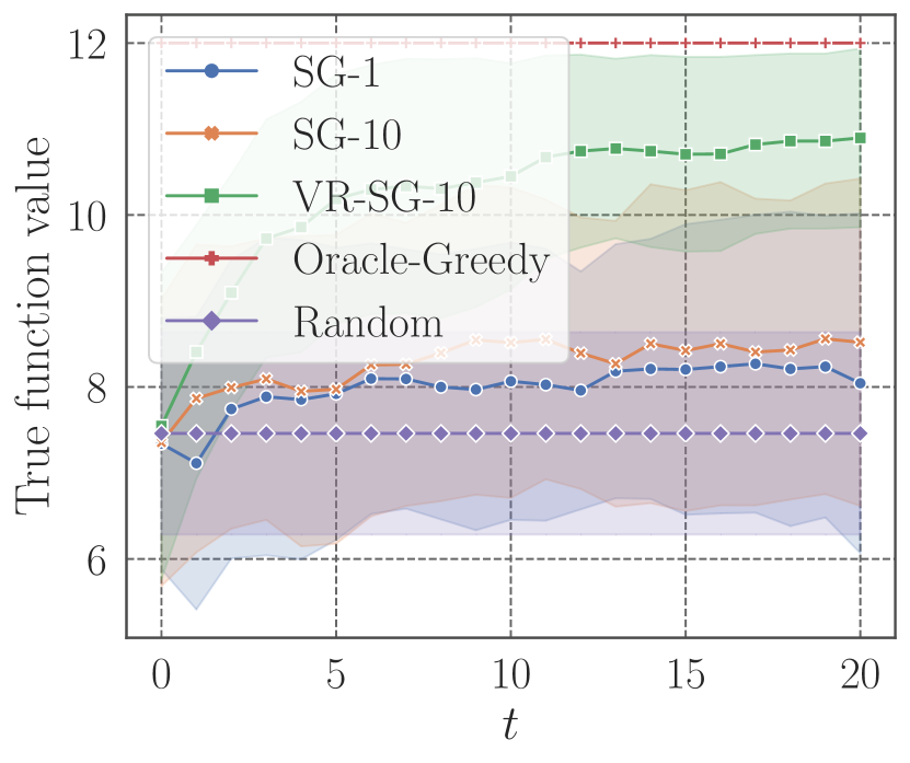
(b) Noise-free

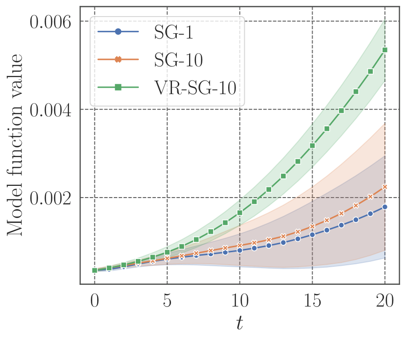
(c) Noisy

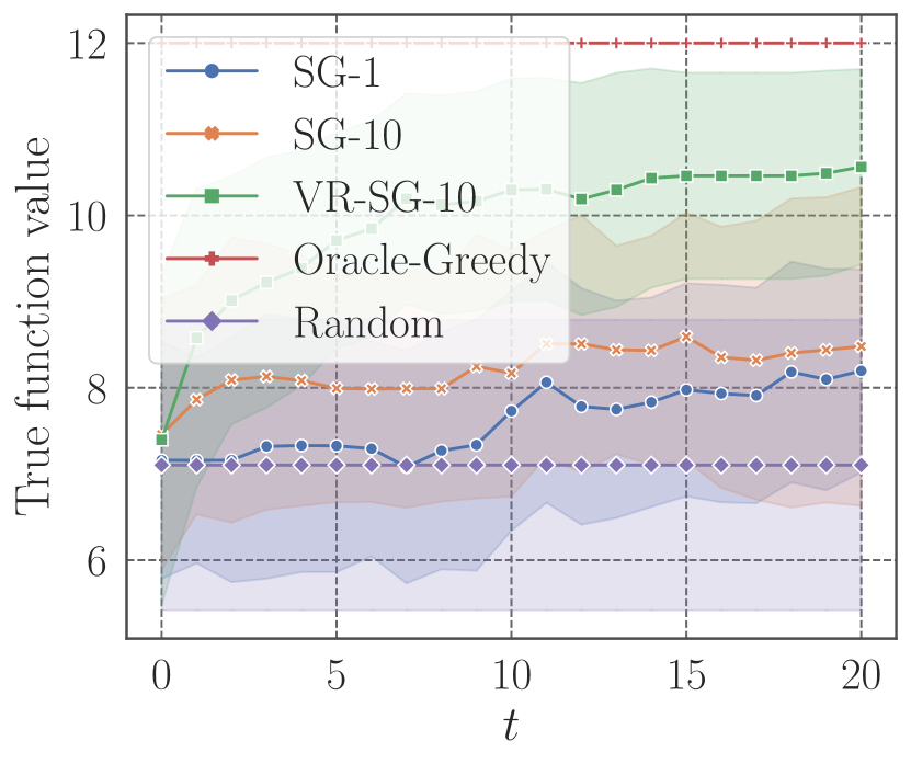
(d) Noisy

Figure 2: Mode and true function values for noise-free (upper) and noisy (lower) settings.

We consider a situation where we make contact with business leaders to make influences on their companies. We use the corporate leadership network dataset of KONECT [6, 35], which contains person–company leadership information between $20$ people and $24$ companies; the companies are indexed with $i=1,\dots,24$. We let each $v\in V$ represent a person, who is associated with a subset of companies $I_{v}\subseteq\{1,\dots,24\}$. We define $I_{X}\coloneqq\bigcup_{v\in X}I_{v}$ for every $X\subseteq V$. We express the importance of the $i$-th company with a non-negative weight $w_{i}$; we let $w_{1}=w_{3}=\dots=w_{23}=1$ and $w_{2}=w_{4}=\cdots=w_{24}=0.1$. We use the weighted coverage function as an unknown true function: $\hat{f}(X)\coloneqq\sum_{i\in I_{X}}w_{i}$. We separate the $20$ people into two groups of $10$ people, and we choose up to two people from each group; i.e., $(V,\mathcal{I})$ forms a partition matroid.

As a model function, $f(\cdot,{\text{{\boldmath$\mathrm{\theta}$}}})$, we use a deep submodular function that forms a $2$-layer NN. We set the hidden-layer size at $50$ and use sigmoid activation functions. We set initial NN parameters $\mathrm{\theta}$ at non-negative values drawn uniformly at random from $[0,0.01]$.

For $t=1,\dots,20$, we perform Smoothed Greedy $N$ times with objective function $f(\cdot,{\text{{\boldmath$\mathrm{\theta}$}}})$; we thus obtain $S_{1},\dots,S_{N}\in\mathcal{I}$. We then query $\hat{f}(S_{1}),\dots,\hat{f}(S_{N})$ values, with which we compute the gradient estimator, and we update $\mathrm{\theta}$ by using Adam with learning rate $10^{-3}$. In each $t$-th round, we evaluate the quality of the trained model, $f(\cdot,{\text{{\boldmath$\mathrm{\theta}$}}})$, as follows: we obtain $S\in\mathcal{I}$ by applying the greedy algorithm to $f(\cdot,{\text{{\boldmath$\mathrm{\theta}$}}})$, and compute model function value $f(S,{\text{{\boldmath$\mathrm{\theta}$}}})$ and true function value $\hat{f}(S)$. We also consider a noisy setting where observed $\hat{f}(S_{j})$ values are perturbed with random variables drawn from the standard normal distribution. We here use the entropy function with $\epsilon=0.02$ as a regularization function of Smoothed Greedy.

As in Section 5.2, (VR-)SG-$N$ stands for (variance-reduced) Smoothed Greedy with $N$ samples. We compare the true function values of (VR-)SG-$N$ with those of two methods: Oracle-Greedy and Random. Oracle-Greedy is the greedy algorithm directly applied to $\hat{f}(\cdot)$, which we assume to be unknown in this setting; we use Oracle-Greedy to see what if we had full access to the unknown true $\hat{f}(\cdot)$. Random returns $X\in\mathcal{I}$ by randomly choosing two people from each of the two groups.

Figure 2 presents the means and standard deviations of the model and true function values over $30$ runs. We see that, by updating the model function, we can increase the true function values. As indicated by the results of SG-$1$, if even once we can query $\hat{f}(\cdot)$ value in each round, we can do better than Random. With more queries and the variance reduction method, we can achieve higher true function values. The results suggest that our method is useful for learning and maximizing submodular functions when very limited prior knowledge and feedback are available.

Appendix F Differentiable stochastic greedy algorithm

We show that our framework can be used for making the stochastic greedy algorithm [38] differentiable, which is a faster randomized variant of the greedy algorithm. In this section, we focus on the cardinality constrained case.

Algorithm 2 presents the smoothed version of the stochastic greedy algorithm, which we call Stochastic Smoothed Greedy. The only difference from Smoothed Greedy (Algorithm 1) is in Step 3, where we sample ${n_{k}}$ elements uniformly at random without replacement from $V\backslash S$ . In what follows, we let ${n_{k}}=\left\lceil{\frac{n}{K}\ln\frac{1}{\varepsilon}}\right\rceil$ for every $k=1,\dots,K$, where $\varepsilon\in(0,1)$ is a hyper-parameter; this plays a role of controlling the speed–accuracy trade-off.

As with the original stochastic greedy algorithm, Stochastic Smoothed Greedy requires only $\mathrm{O}(n\ln{1}/{\varepsilon})$ evaluations of $f(\cdot,{\text{{\boldmath$\mathrm{\theta}$}}})$, while Smoothed Greedy requires $\mathrm{O}(nK)$. Moreover, as explained in Section F.2, the gradient estimator for Stochastic Smoothed Greedy can be computed more efficiently than that for Smoothed Greedy. Therefore, Stochastic Smoothed Greedy is useful when $n$ and $K$ are large and/or the evaluation of $f(\cdot,{\text{{\boldmath$\mathrm{\theta}$}}})$ is costly. Below we prove the approximation guarantee of Stochastic Smoothed Greedy, and explain how to compute gradient estimators. We also present experiments to see the empirical speed–accuracy trade-off.

Algorithm 2 Stochastic Smoothed Greedy

1:$S\leftarrow\emptyset$

2:for $k=1,2\dots,K$ do

3:     ${U_{k}}=\{u_{1},\dots,u_{{n_{k}}}\}\leftarrow\text{ ${n_{k}}$ elements chosen from $V\backslash S$ uniformly at random}$

4:     ${\text{{\boldmath$\mathrm{g}$}}}_{k}({\text{{\boldmath$\mathrm{\theta}$}}})=(g_{k}(u_{1},{\text{{\boldmath$\mathrm{\theta}$}}}),\dots,g_{k}(u_{n_{k}},{\text{{\boldmath$\mathrm{\theta}$}}}))\leftarrow(f_{{S}}({u_{1}},{{\text{{\boldmath$\mathrm{\theta}$}}}}),\dots,f_{{S}}({u_{{n_{k}}}},{{\text{{\boldmath$\mathrm{\theta}$}}}}))$

5:     ${\text{{\boldmath$\mathrm{p}$}}}_{k}({\text{{\boldmath$\mathrm{\theta}$}}})=(p_{k}(u_{1},{\text{{\boldmath$\mathrm{\theta}$}}}),\dots,p_{k}(u_{n_{k}},{\text{{\boldmath$\mathrm{\theta}$}}}))\leftarrow\operatorname*{argmax}_{{\text{{\boldmath$\mathrm{p}$}}}\in\Delta^{{n_{k}}}}\{\left\langle{{\text{{\boldmath$\mathrm{g}$}}}_{k}({\text{{\boldmath$\mathrm{\theta}$}}}),{\text{{\boldmath$\mathrm{p}$}}}}\right\rangle-\Omega_{k}({\text{{\boldmath$\mathrm{p}$}}})\}$

6:     $s_{k}\leftarrow u\in{U_{k}}$ with probability $p_{k}(u,{\text{{\boldmath$\mathrm{\theta}$}}})$

7:     $S\leftarrow S\cup\{s_{k}\}$ return $S$

F.1 Approximation guarantee

We prove that Algorithm 2 returns solution $S$ that satisfies the following approximation guarantee for the cardinality constrained case.

Theorem 3.

If ${n_{k}}\geq\frac{n}{K}\ln\frac{1}{\varepsilon}$ for $k=1,\dots,K$, we have $\mathbb{E}[f(S,{\text{{\boldmath$\mathrm{\theta}$}}})]\geq(1-1/\mathrm{e}-\varepsilon)f(O,{\text{{\boldmath$\mathrm{\theta}$}}})-\delta K$.

Proof.

As with the proofs in Appendix B, we omit $\mathrm{\theta}$ and use $S_{k}$ to denote the solution obtained in the $k$-th step ($k=0,\dots,K$). We take all random quantities to be conditioned on the realization of the $(k-1)$-th step. Once ${U_{k}}$ is fixed in Step 3, we can obtain the following inequality from 1:

$$\mathbb{E}[f_{{S_{k-1}}}({s_{k}})\mathrel{|}{U_{k}}]\geq f_{{S_{k-1}}}({s^{*}_{k}})-\delta,$$ (A18)

where $s^{*}_{k}\in\operatorname*{argmax}_{u\in{U_{k}}}f_{{S_{k-1}}}({u})$ and $\mathbb{E}[\cdot\mathrel{|}{U_{k}}]$ denotes the expectation conditioned on ${U_{k}}$. By taking the expectation over all possible choices of ${U_{k}}$, we obtain

$$\mathbb{E}[f(S_{k})]-f(S_{k-1})=\mathbb{E}[f_{{S_{k-1}}}({s_{k}})]\geq\mathbb{E}[f_{{S_{k-1}}}({s^{*}_{k}})]-\delta.$$ (A19)

Note that here, $s^{*}_{k}$ is a random variable representing an element, which the original stochastic greedy algorithm adds to the current solution. As proved in [38], if ${n_{k}}\geq\frac{n}{K}\ln\frac{1}{\varepsilon}$, we have

$$\mathbb{E}[f_{{S_{k-1}}}({s^{*}_{k}})]\geq\frac{1-\varepsilon}{K}(f(O\cup S_{k-1})-f(S_{k-1})).$$ (A20)

By substituting this inequality into (A19) and taking the expectation over all possible realizations of $S_{k-1}$, we obtain

$$\mathbb{E}[f(S_{k})]-\mathbb{E}[f(S_{k-1})]\geq\frac{1-\varepsilon}{K}(\mathbb{E}[f(O\cup S_{k-1})]-\mathbb{E}[f(S_{k-1})])-\delta,$$ (A21)

which holds for $k=1,\dots,K$. Therefore, by induction, we obtain the theorem as follows:

$$\mathbb{E}[f(S)]\geq\left(1-\left(1-\frac{1-\varepsilon}{K}\right)^{K}\right)f(O)-\delta\sum_{k=0}^{K-1}\left(1-\frac{1-\varepsilon}{K}\right)^{k}\geq\left(1-\frac{1}{\mathrm{e}}-\varepsilon\right)f(O)-\delta K,$$

where we used $\mathbb{E}[f(O\cup S_{k-1})]\geq f(O)$, $f(\emptyset)=0$, and $\mathbb{E}[f(S)]=\mathbb{E}[f(S_{K})]$. ∎

F.2 Gradient estimation

We show how to compute gradient estimators for Stochastic Smoothed Greedy. As with the case of Smoothed Greedy, outputs of Stochastic Smoothed Greedy are distributed over $\mathscr{S}_{\leq K}$. Therefore, the score-function gradient estimator can be computed by sampling outputs as in Section 3, i.e.,

$$\nabla_{\text{{\boldmath$\mathrm{\theta}$}}}\mathbb{E}_{S\sim p({\text{{\boldmath$\mathrm{\theta}$}}})}[Q(S)]\approx\frac{1}{N}\sum_{j=1}^{N}Q(S_{j})\nabla_{\text{{\boldmath$\mathrm{\theta}$}}}\ln p(S_{j},{\text{{\boldmath$\mathrm{\theta}$}}})\quad\text{where}\quad S_{j}=(s_{1},\dots,s_{|S_{j}|})\sim p({\text{{\boldmath$\mathrm{\theta}$}}}).$$ (A22)

Note that here $p({\text{{\boldmath$\mathrm{\theta}$}}})$ denotes the output distribution of the Stochastic Smoothed Greedy; more precisely, for ${\text{{\boldmath$\mathrm{p}$}}}_{1}({\text{{\boldmath$\mathrm{\theta}$}}}),\dots,{\text{{\boldmath$\mathrm{p}$}}}_{K}({\text{{\boldmath$\mathrm{\theta}$}}})$ and solution $S=\{s_{1},\dots,s_{K}\}$ computed by Algorithm 2, we let $p(S,{\text{{\boldmath$\mathrm{\theta}$}}})=\prod_{k=1}^{|S|}p_{k}(s_{k},{\text{{\boldmath$\mathrm{\theta}$}}})$, where $p_{k}(s_{k},{\text{{\boldmath$\mathrm{\theta}$}}})$ is the entry of ${\text{{\boldmath$\mathrm{p}$}}}_{k}({\text{{\boldmath$\mathrm{\theta}$}}})$ corresponding to $s_{k}\in{U_{k}}$. We can compute $\nabla_{\text{{\boldmath$\mathrm{\theta}$}}}\ln p(S_{j},{\text{{\boldmath$\mathrm{\theta}$}}})$ in the same manner as in Section 3.

Remember that the computation of $\nabla_{\text{{\boldmath$\mathrm{\theta}$}}}\ln p(S_{j},{\text{{\boldmath$\mathrm{\theta}$}}})$ involves the following differentiation based on the chain rule: $\nabla_{\text{{\boldmath$\mathrm{\theta}$}}}{\text{{\boldmath$\mathrm{p}$}}}_{k}({\text{{\boldmath$\mathrm{\theta}$}}})=\nabla_{{\text{{\boldmath$\mathrm{g}$}}}_{k}}{\text{{\boldmath$\mathrm{p}$}}}_{k}({\text{{\boldmath$\mathrm{g}$}}}_{k})\cdot\nabla_{\text{{\boldmath$\mathrm{\theta}$}}}{\text{{\boldmath$\mathrm{g}$}}}_{k}({\text{{\boldmath$\mathrm{\theta}$}}})$. Here, the dimensionality of ${\text{{\boldmath$\mathrm{p}$}}}_{k}$ and ${\text{{\boldmath$\mathrm{g}$}}}_{k}$ is at most ${n_{k}}=\left\lceil{\frac{n}{K}\ln\frac{1}{\varepsilon}}\right\rceil$, while it is up to $n$ in the case of Smoothed Greedy. Therefore, Stochastic Smoothed Greedy is effective for speeding up the computation of gradient estimators.

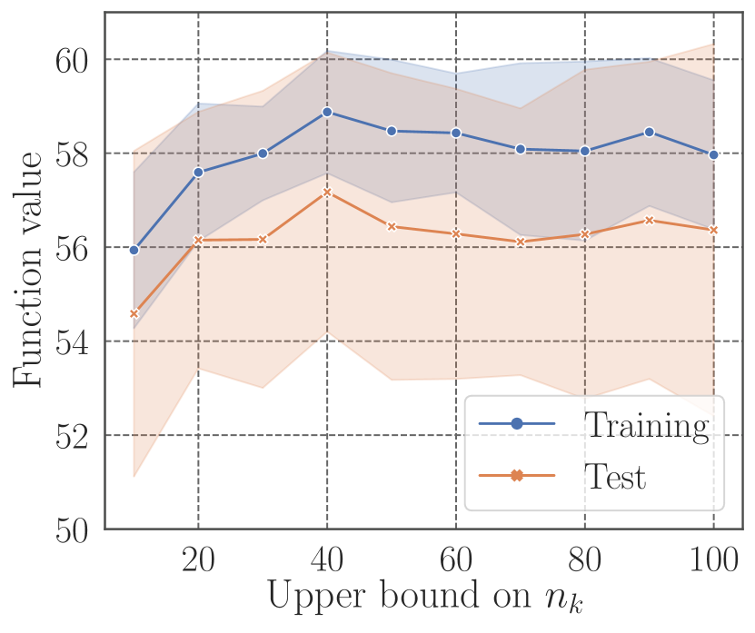
(a) Training and test scores

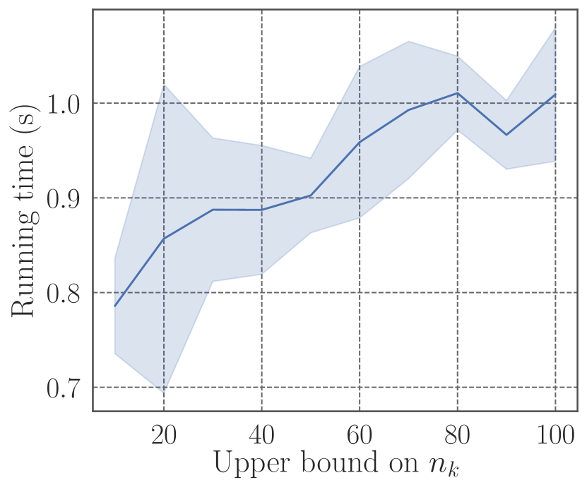
(b) Solution computation

(c) Gradient estimation

Figure 3: (a): Objective function values achieved for the training and test instances. (b): Running times of Stochastic Smoothed Greedy for updating $\mathrm{w}$ once (summation over $200$ runs). (c): Running times of the gradient-estimator computation.

F.3 Experiments

We study the empirical performance of Stochastic Smoothed Greedy. We use the same settings as those of the decision-focused learning experiments with $K=10$ (see, Section 5.2), where we have $n=100$. We apply the Stochastic Smoothed Greedy version of VR-SG-$10$ to the instances. We consider various upper-bound values, $10,20,\dots,100$, on ${n_{k}}$; that is, in Step 3 of Algorithm 2, we set ${n_{k}}$ at the upper-bound value if it is less than $|V\backslash S|$ and at $|V\backslash S|$ otherwise.

We evaluate objective function values with training and test instances for each upper bound on ${n_{k}}$, where we calculate the means and standard deviations over $30$ training/test splits as in Section 5.2. We also observe running times required for computing solutions with Stochastic Smoothed Greedy and estimating gradients. More precisely, we measure those times taken for once updating the predictive-model parameter, $\mathrm{w}$; since the mini-batch size is $20$ and we perform $N=10$ trials, we take the sum of times over $200$ runs as the running time of Stochastic Smoothed Greedy. In this experiment, $\mathrm{w}$ is updated $600$ times in total; we have $80/20=4$ mini-batches for each of $5$ epochs, and we consider $30$ random training/test splits, hence $4\times 5\times 30=600$. The running times of Stochastic Smoothed Greedy and gradient estimation will be indicated with means and standard deviations over the $600$ iterations.

As shown in Figure 3, even if ${n_{k}}$ decreases, the objective function values do not drop so much with both training and test instances; rather, the highest values are achieved with ${n_{k}}=40$. The results imply that the stochastic greedy algorithm remains empirically effective even if it is smoothed with our framework. Figures 3 and 3 confirm that by decreasing ${n_{k}}$, we can reduce the running times required for computing solutions and estimating gradients. In this experimental setting, since the instance size is not so large and objective function values can be efficiently computed via matrix-vector products, the run-time overhead becomes dominant; this makes the degree of the speed-up yielded by decreasing ${n_{k}}$ appears less significant. However, when instance sizes are larger and evaluations of objective functions are more costly, the speed-up achieved by using Stochastic Smoothed Greedy becomes more significant.

References

- Abernethy et al. [2016] J. Abernethy, C. Lee, and A. Tewari. Perturbation techniques in online learning and optimization. In Perturbations, Optimization, and Statistics. MIT Press, 2016.
- Alon et al. [2012] N. Alon, I. Gamzu, and M. Tennenholtz. Optimizing budget allocation among channels and influencers. In Proceedings of the 21st International Conference on World Wide Web, pages 381–388. ACM, 2012.
- Amos and Kolter [2017] B. Amos and J. Z. Kolter. OptNet: Differentiable optimization as a layer in neural networks. In Proceedings of the 34th International Conference on Machine Learning, volume 70, pages 136–145. PMLR, 2017.
- Balcan and Harvey [2011] M.-F. Balcan and N. J. A. Harvey. Learning submodular functions. In Proceedings of the 43rd Annual ACM Symposium on Theory of Computing, pages 793–802. ACM, 2011.
- Balkanski and Singer [2018] E. Balkanski and Y. Singer. The adaptive complexity of maximizing a submodular function. In Proceedings of the 50th Annual ACM Symposium on Theory of Computing, pages 1138–1151. ACM, 2018.
- Barnes and Burkett [2010] R. Barnes and T. Burkett. Structural redundancy and multiplicity in corporate networks. Connect., 30(2):4–20, 2010.
- Baydin et al. [2018] A. G. Baydin, B. A. Pearlmutter, A. A. Radul, and J. M. Siskind. Automatic differentiation in machine learning: a survey. J. Mach. Learn. Res., 18(153):1–43, 2018.
- Berthet et al. [2020] Q. Berthet, M. Blondel, O. Teboul, M. Cuturi, J.-P. Vert, and F. Bach. Learning with differentiable perturbed optimizers. arXiv preprint arXiv:2002.08676, 2020.
- Bertsekas [2016] D. P. Bertsekas. Nonlinear Programming. Athena Scientific, 3rd edition, 2016.
- Bertsimas [1988] D. Bertsimas. Probabilistic Combinatorial Optimization Problems. PhD thesis, Massachusetts Institute of Technology, 1988.
- Calinescu et al. [2011] G. Calinescu, C. Chekuri, M. Pál, and J. Vondrák. Maximizing a monotone submodular function subject to a matroid constraint. SIAM J. Comput., 40(6):1740–1766, 2011.
- Cuturi [2013] M. Cuturi. Sinkhorn distances: Lightspeed computation of optimal transport. In Advances in Neural Information Processing Systems 26, pages 2292–2300. Curran Associates, Inc., 2013.
- Cuturi et al. [2019] M. Cuturi, O. Teboul, and J.-P. Vert. Differentiable ranking and sorting using optimal transport. In Advances in Neural Information Processing Systems 32, pages 6861–6871. Curran Associates, Inc., 2019.
- Djolonga and Krause [2017] J. Djolonga and A. Krause. Differentiable learning of submodular models. In Advances in Neural Information Processing Systems 30, pages 1013–1023. Curran Associates, Inc., 2017.
- Dolhansky and Bilmes [2016] B. W. Dolhansky and J. A. Bilmes. Deep submodular functions: Definitions and learning. In Advances in Neural Information Processing Systems 29, pages 3404–3412. Curran Associates, Inc., 2016.
- Dontchev and Rockafellar [2014] A. L. Dontchev and R. T. Rockafellar. Implicit Functions and Solution Mappings. Springer, 2nd edition, 2014.
- Donti et al. [2017] P. Donti, B. Amos, and J. Z. Kolter. Task-based end-to-end model learning in stochastic optimization. In Advances in Neural Information Processing Systems 30, pages 5484–5494. Curran Associates, Inc., 2017.
- Feige [1998] U. Feige. A threshold of ln for approximating set cover. J. ACM, 45(4):634–652, 1998.
- Ferber et al. [2020] A. Ferber, B. Wilder, B. Dilina, and M. Tambe. MIPaaL: Mixed integer program as a layer. In Proceedings of the 34th AAAI Conference on Artificial Intelligence (to appear), 2020. arXiv:1907.05912.
- Fisher et al. [1978] M. L. Fisher, G. L. Nemhauser, and L. A. Wolsey. An analysis of approximations for maximizing submodular set functions–II. In Polyhedral combinatorics, pages 73–87. Springer, 1978.
- Gal and Greenberg [2012] T. Gal and H. J. Greenberg. Advances in Sensitivity Analysis and Parametric Programming, volume 6. Springer, 2012.
- Ghosh et al. [2000] D. Ghosh, N. Chakravarti, and G. Sierksma. Sensitivity analysis of the greedy heuristic for binary knapsack problems. Research Report 00A18, University of Groningen, Research Institute SOM (Systems, Organisations and Management), 2000.
- Glynn [1990] P. W. Glynn. Likelihood ratio gradient estimation for stochastic systems. Commun. ACM, 33(10):75–84, 1990.
- Greensmith et al. [2004] E. Greensmith, P. L. Bartlett, and J. Baxter. Variance reduction techniques for gradient estimates in reinforcement learning. J. Mach. Learn. Res., 5(Nov):1471–1530, 2004.
- Griewank and Walther [2008] A. Griewank and A. Walther. Evaluating Derivatives. SIAM, 2nd edition, 2008.
- Gumbel [1954] E. J. Gumbel. Statistical theory of extreme values and some practical applications: A series of lectures. US Govt. Print. Office, 33, 1954.
- Gusfield [1980] D. M. Gusfield. Sensitivity Analysis for Combinatorial Optimization. PhD thesis, University of California, Berkeley, 1980.
- Harper and Konstan [2015] F. M. Harper and J. A. Konstan. The MovieLens datasets: History and context. ACM Trans. Interact. Intell. Syst., 5(4):19:1–19:19, 2015. URL https://grouplens.org/datasets/movielens/100k/.
- Hassani et al. [2017] H. Hassani, M. Soltanolkotabi, and A. Karbasi. Gradient methods for submodular maximization. In Advances in Neural Information Processing Systems 30, pages 5841–5851. Curran Associates, Inc., 2017.
- Jang et al. [2017] E. Jang, S. Gu, and B. Poole. Categorical reparameterization with Gumbel-Softmax. In International Conference on Learning Representations, 2017.
- Kakade and Lee [2018] S. M. Kakade and J. D. Lee. Provably correct automatic subdifferentiation for qualified programs. In Advances in Neural Information Processing Systems 31, pages 7125–7135. Curran Associates, Inc., 2018.
- Kalyan et al. [2019] A. Kalyan, P. Anderson, S. Lee, and D. Batra. Trainable decoding of sets of sequences for neural sequence models. In Proceedings of the 36th International Conference on Machine Learning, volume 97, pages 3211–3221. PMLR, 2019.
- Kannan et al. [2018] S. Kannan, J. H. Morgenstern, A. Roth, B. Waggoner, and Z. S. Wu. A smoothed analysis of the greedy algorithm for the linear contextual bandit problem. In Advances in Neural Information Processing Systems 31, pages 2227–2236. Curran Associates, Inc., 2018.
- Kleijnen and Rubinstein [1996] J. P. C. Kleijnen and R. Y. Rubinstein. Optimization and sensitivity analysis of computer simulation models by the score function method. European J. Oper. Res., 88(3):413–427, 1996.
- Kunegis [2013] J. Kunegis. KONECT: The Koblenz Network Collection. In Proceedings of the 22nd International Conference on World Wide Web, pages 1343–1350. ACM, 2013. URL http://konect.uni-koblenz.de/networks/brunson_corporate-leadership.
- Maddison et al. [2017] C. J. Maddison, A. Mnih, and Y. W. Teh. The Concrete distribution: A continuous relaxation of discrete random variables. In International Conference on Learning Representations, 2017.
- Mestre [2006] J. Mestre. Greedy in approximation algorithms. In Proceedings of the 17th Annual European Symposium on Algorithms, pages 528–539. Springer, 2006.
- Mirzasoleiman et al. [2015] B. Mirzasoleiman, A. Badanidiyuru, A. Karbasi, J. Vondrák, and A. Krause. Lazier than lazy greedy. In Proceedings of the 29th AAAI Conference on Artificial Intelligence, pages 1812–1818. AAAI Press, 2015.
- Mirzasoleiman et al. [2016] B. Mirzasoleiman, A. Badanidiyuru, and A. Karbasi. Fast constrained submodular maximization: Personalized data summarization. In Proceedings of the 33rd International Conference on Machine Learning, volume 48, pages 1358–1367. PMLR, 2016.
- Mohamed et al. [2019] S. Mohamed, M. Rosca, M. Figurnov, and A. Mnih. Monte Carlo gradient estimation in machine learning. arXiv preprint arXiv:1906.10652, 2019.
- Nemhauser and Wolsey [1978] G. L. Nemhauser and L. A. Wolsey. Best algorithms for approximating the maximum of a submodular set function. Math. Oper. Res., 3(3):177–188, 1978.
- Nemhauser et al. [1978] G. L. Nemhauser, L. A. Wolsey, and M. L. Fisher. An analysis of approximations for maximizing submodular set functions–I. Math. Program., 14(1):265–294, 1978.
- Paszke et al. [2017] A. Paszke, S. Gross, S. Chintala, G. Chanan, E. Yang, Z. DeVito, Z. Lin, A. Desmaison, L. Antiga, and A. Lerer. Automatic differentiation in PyTorch. In NIPS 2017 Workshop Autodiff, 2017.
- Peyrard [2019] M. Peyrard. Principled Approaches to Automatic Text Summarization. PhD thesis, Technische Universität, 2019.
- Pogančić et al. [2020] M. V. Pogančić, A. Paulus, V. Musil, G. Martius, and M. Rolinek. Differentiation of blackbox combinatorial solvers. In International Conference on Learning Representations, 2020.
- Powers et al. [2018] T. Powers, R. Fakoor, S. Shakeri, A. Sethy, A. Kainth, A. Mohamed, and R. Sarikaya. Differentiable greedy networks. arXiv preprint arXiv:1810.12464, 2018.
- Rockafellar and Wets [1998] R. T. Rockafellar and R. J-B Wets. Variational Analysis, volume 317. Springer, 1998.
- Rosenfeld et al. [2018] N. Rosenfeld, E. Balkanski, A. Globerson, and Y. Singer. Learning to optimize combinatorial functions. In Proceedings of the 35th International Conference on Machine Learning, volume 80, pages 4374–4383. PMLR, 2018.
- Rubinstein et al. [1996] R. Y. Rubinstein, A. Shapiro, and S. Uryasev. The score function method. Encyclopedia of Management Sciences, pages 1363–1366, 1996.
- Staib et al. [2019] M. Staib, B. Wilder, and S. Jegelka. Distributionally robust submodular maximization. In Proceedings of the 22nd International Conference on Artificial Intelligence and Statistics, volume 89, pages 506–516. PMLR, 2019.
- Stechlinski et al. [2018] P. Stechlinski, K. A. Khan, and P. I. Barton. Generalized sensitivity analysis of nonlinear programs. SIAM J. Optim., 28(1):272–301, 2018.
- Tschiatschek et al. [2018] S. Tschiatschek, A. Sahin, and A. Krause. Differentiable submodular maximization. In Proceedings of the 27th International Joint Conference on Artificial Intelligence, pages 2731–2738. IJCAI Organization, 2018.
- Tucker et al. [2017] G. Tucker, A. Mnih, C. J. Maddison, J. Lawson, and J. Sohl-Dickstein. REBAR: Low-variance, unbiased gradient estimates for discrete latent variable models. In Advances in Neural Information Processing Systems 30, pages 2627–2636. Curran Associates, Inc., 2017.
- Varma and Yoshida [2019] N. Varma and Y. Yoshida. Average sensitivity of graph algorithms. arXiv preprint arXiv:1904.03248, 2019.
- Wang et al. [2019] P.-W. Wang, P. Donti, B. Wilder, and Z. Kolter. SATNet: Bridging deep learning and logical reasoning using a differentiable satisfiability solver. In Proceedings of the 36th International Conference on Machine Learning, volume 97, pages 6545–6554. PMLR, 2019.
- Wei et al. [2015] K. Wei, R. Iyer, and J. Bilmes. Submodularity in data subset selection and active learning. In Proceedings of the 32nd International Conference on Machine Learning, volume 37, pages 1954–1963. PMLR, 2015.
- Wilder et al. [2019a] B. Wilder, B. Dilkina, and M. Tambe. Melding the data-decisions pipeline: Decision-focused learning for combinatorial optimization. In Proceedings of the 33rd AAAI Conference on Artificial Intelligence, pages 1658–1665. AAAI Press, 2019a.
- Wilder et al. [2019b] B. Wilder, E. Ewing, B. Dilkina, and M. Tambe. End to end learning and optimization on graphs. In Advances in Neural Information Processing Systems 32, pages 4672–4683. Curran Associates, Inc., 2019b.
- Williams [1992] R. J. Williams. Simple statistical gradient-following algorithms for connectionist reinforcement learning. Mach. Learn., 8(3):229–256, 1992.
- Zhang et al. [2019] M. Zhang, L. Chen, H. Hassani, and A. Karbasi. Online continuous submodular maximization: From full-information to bandit feedback. In Advances in Neural Information Processing Systems 32, pages 9210–9221. Curran Associates, Inc., 2019.