Quantum black holes in the horizon quantum mechanics model
at the Large Hadron Collider

Abstract

Quantum black hole production at the Large Hadron Collider is investigated using the horizon quantum mechanics model. This model has novel implications for how black holes might be observed in collider experiments. Black hole production is predicted to be possible below the Planck scale, thus leading to the intriguing possibility that black holes could be produced even if the Planck scale is slightly above the collider center of mass energy. In addition, the usual anticipated resonance in the black hole mass distribution is significantly widened in this model. For values of the Planck scale above the current lower limits, the shape of the black hole mass distribution is almost independent of the Planck scale and depends more on the number of extra dimensions. These model features suggest the need for alternative search strategies in collider experiments.

I Introduction

Low-scale gravity provides an interesting possibility for gaining insight into the hierarchy problem. A wide variety of models based on different paradigms [1, 2, 3] have been proposed. A speculative, but intriguing, possibility of most models is the production of quantum black holes in hadron colliders [4, 5].

The cross section for black hole production is typically chosen to be the classical geometric form $\hat{\sigma}\approx\pi r_{\mathrm{g}}^{2}$, where $r_{\mathrm{g}}$ is the gravitational radius which is a function of the black hole mass $M$ and depends on the fundamental parameters of the model. In the large extra dimensions paradigm proposed in Ref. [1, 2], the model parameters are the higher-dimensional Planck scale $M_{D}$ and total number of space-time dimensions $D$. We will consider the case of a tensionless non-rotating spherically symmetric solution for the gravitational radius [6].

In proton–proton collisions, only a fraction of the total center of mass energy $\sqrt{s}$ is available in the hard-scatter process. We define $sx_{a}x_{b}\equiv s\tau\equiv\hat{s}$, where $x_{a}$ and $x_{b}$ are the fractional energies of the two colliding partons (assumed massless) relative to the proton energies. The full particle-level cross section $\sigma$ is obtained from the parton-level cross section $\hat{\sigma}$ by using [7]

$$\sigma_{pp\to\mathrm{BH+X}}(s) = \sum_{a,b}\int_{M^{2}/s}^{1}d\tau\int_{\tau}^{1}\frac{dx}{x}f_{a}\left(\frac{\tau}{x}\right)f_{b}(x)\Theta(M-M_{\mathrm{th}})\hat{\sigma}_{\mathrm{ab\to BH}}(\hat{s}=M^{2})\,,$$ (1)

where $a$ and $b$ are the parton types in the two protons, and $f_{a}$ and $f_{b}$ are parton distribution functions (PDFs) for the proton. The sum is over all possible quark and gluon pairings. While several pre-factors to the cross section have been suggested (see Ref. [7] for a summary) they are not important for this study and will not be considered.

The usual ansatz is that black holes can not be produced with $M$ below some minimum mass threshold $M_{\mathrm{th}}$. This is emphasized by the use of the Heaviside step function $\Theta$ in Eq. (1). The value of $M_{\mathrm{th}}$ is typically taken to be $M_{D}$ for quantum black holes or a few times $M_{D}$ for classical black holes. Unfortunately, results depend on the subjective choice of the $M_{\mathrm{th}}$ cutoff.

A modification to the typical model of black hole formation in hadron colliders is made by the horizon quantum mechanics (HQM) model [8, 9]. The wave function for a localized massive particle (source) is taken to be a spherically symmetric Gaussian wave packet in $(D-1)$ spatial dimensions of width $\ell$. It is postulated that the form of the wave packet in momentum space is also a Gaussian with width $\Delta=\hbar/\ell$. The simplest case for black hole formation is considered; a $D$-dimensional Schwarzschild metric and its classical horizon of radius $R_{D}(M)$. The relativistic mass-shell relation in flat space $E^{2}=p^{2}+m^{2}$ is assumed, where the energy $E$ of the particle is expressed in terms of the horizon radius $r_{\mathrm{H}}=R_{D}(E)$ and $m$ is the rest mass of the source. The momentum-space wave function can then be written in terms of the horizon radius and normalized to give the horizon wave function $\psi_{\mathrm{H}}(r_{\mathrm{H}})$. The horizon wave function is used to calculate the probability $P_{\,\mathrm{S}}(r<r_{\mathrm{H}})$ that the particle is inside a $(D-1)$-ball of radius $r_{\mathrm{H}}$ and the probability density $\mathcal{P}_{\,\mathrm{H}}(r_{\mathrm{H}})$ that the radius of the horizon equals $r_{\mathrm{H}}$. In this case, the black hole probability depends on the Gaussian width $\ell$, particle mass $m$, and number of spatial dimensions $D$. It is further assumed that $\ell=M_{D}\ell_{D}/m$ is the Compton wavelength of the source, which represents the minimum uncertainty in its size, so that $\Delta=m$, and the probability only depends on $m$ and the number of dimensions $D$. The system exhibits properties of a black hole when the source is located within the quantized horizon, with the probability of the system being a black hole given by

$$P_{\,\mathrm{BH}}=\int_{0}^{\infty}P_{\,\mathrm{S}}(r<r_{\mathrm{H}})\mathcal{P}_{\,\mathrm{H}}(r_{\mathrm{H}})dr_{\mathrm{H}}\,.$$ (2)

Explicit expressions of these probabilities are giving in Ref. [8, 9]. Qualitatively, the use of the HQM probability in the calculation of the proton–proton cross section is akin to replacing the step function located at $M_{\mathrm{th}}$ with a sigmoid-like function that varies with $M/M_{D}$ and depends on $D$.

The ingredients that go into deriving Eq. (2) are not free of assumptions. In addition, using standard quantum mechanics in the strong gravity regime is ill defined and the formalism is not free of problems. The idea of improving the geometrical cross section by a smoothed step function is not new [10]. Using guiding physical principles similar results to Eq. (2) can be obtained on empirical grounds [10].

The common phenomenology of semi-classical microscopic black holes is not important in this work. Such objects have significant entropy and Hawking evaporate. The evaporation process occurs when the mass of the black hole is well above the Planck scale and thus not close to where HQM effects are important. We thus consider, so called, quantum black holes (QBH), where the object has an event horizon but negligible entropy, and behaves more like a particle in its decay to a few-body – two in our case – final state. Such objects by definition have mass close to the Planck scale and are significantly affected by the HQM model.

The purpose of the work presented here is to evaluate the impact of the HQM model on the production of quantum black holes with emphasis on the signatures for experiments at the Large Hadron Collider (LHC). We begin with a brief description of Monte Carlo (MC) event generation in the HQM model, with more details of the implementation described in Appendix A. We discuss the effects of HQM on the total proton–proton cross section and the differential proton–proton cross section as a function of $M$. The possibility of quantum black hole detection in the HQM model in LHC experiments is discussed. A previous publication [11] on this topic made use of ATLAS and CMS results from about 20 fb^-1 of data at $\sqrt{s}=8$ TeV.

We make use of the following conventions. When comparing models, the QBH model refers to the quantum black hole model with Heaviside step function turn-on typically used by ATLAS and CMS searches at $\sqrt{s}$ of 7 TeV [12, 13, 14], 8 TeV [15, 16, 17, 18, 19, 20], and 13 TeV [21, 22, 23, 24, 25, 26, 27, 28] that does not include any HQM effects. The HQM model will be the model with horizon quantum mechanics effects included. The only difference between these two models is their production turn-on behaviour in $M/M_{D}$ for different $D$. The total number of space-time dimensions $D=n+4$, where $n$ is the number of extra dimensions.

II Black hole production probability

For the purpose of cross section calculations along with event generation, the Qbh 3.00 MC quantum black hole event generator is used [30]. In this model [31, 32, 33], we consider tensionless non-rotating black holes. The generator only allows for dominant two-body decay of the QBH states. The leading-order CTEQ6L1 [34] PDF set is used for the hard-scattering process. Considering only two-body decays and using the CTEQ6L1 PDF set are consistent with the ATLAS and CMS experiment’s QBH searches. The default settings in Qbh are used and the proton–proton center of mass energy is set to 13 TeV. The only parameters that are varied are $M_{D}$ and $D$. Cross section calculations in Qbh are independent of the number of events generated. For kinematic distributions, 21000 events were generated for each $(D,M_{D})$ pair. We work at the parton level and do not hadronize the partons or decay the final state particles; a hadron is considered as a single jet. No energy-momentum smearing or detector simulation has been performed. HQM effects are added to the proton–proton cross section by including the factor $P_{\,\mathrm{BH}}$ of Eq. (2) into Eq. (1):

$$\sigma_{pp\to\mathrm{BH+X}}(s) = \sum_{a,b}\int_{M^{2}/s}^{1}d\tau\int_{\tau}^{1}\frac{dx}{x}f_{a}\left(\frac{\tau}{x}\right)f_{b}(x)P_{\,\mathrm{BH}}(M)\hat{\sigma}_{\mathrm{ab\to BH}}(\hat{s}=M^{2})\,,$$ (3)

where $P_{\,\mathrm{BH}}$ requires another numerical integration. The cross section formula is now independent of $M_{\mathrm{th}}$ and the model has one less free parameter.

In order to visualise how the HQM probability varies with $M,M_{D}$, and $D$, we have computed the integral in Eq. (2) explicitly, as shown in Fig. 1.

Figure 1: Horizon quantum mechanics (HQM) probability curves $P_{\,\mathrm{BH}}$ versus black hole mass $M$ relative to the Planck scale $M_{D}$ for selected total number of space-time dimensions $D$. The dashed black line represents the step function used in quantum black hole (QBH) models.

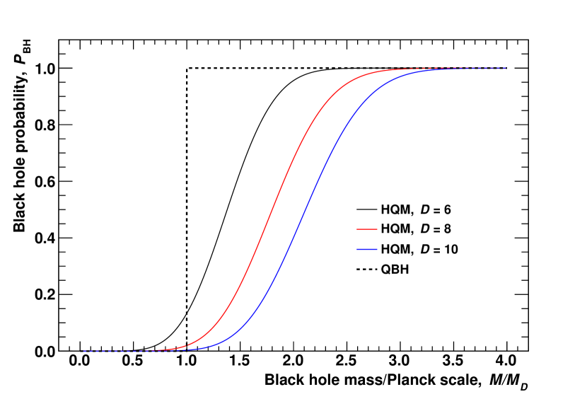
The probability curves suggest some interesting phenomena that are not seen in the QBH model. First, instead of a step function at $M=M_{D}$, the new curves are smooth. The most notable consequence is that there is a finite probability that a black hole can be formed with $M<M_{D}$. Second, we see that the probability for a black hole to be produced near $M_{D}$ is suppressed for high $D$. In other words, one generally expects more black holes to be produced for low $D$. This is at odds with the usual effect of dimensionality in the QBH model, where greater $D$ corresponds to a greater geometric cross section. A third observation is that most of the curve is significantly above the value of $M/M_{D}=1$. And lastly, the slope in the curves at $P_{\,\mathrm{BH}}=0.5$ are not particularly steep.

We can roughly quantify the extent to which the $P_{\,\mathrm{BH}}$ curves create a threshold in the $M$ distribution by considering the midpoint of each curve as the point where $P_{\,\mathrm{BH}}=0.5$. These values are shown in Table 1. For $D=6$, the black hole mass threshold rises to slightly above the usual $M_{D}$ threshold in the QBH model. For $D=10$, the threshold is more than twice $M_{D}$. This means that more dimensions will cause heavy suppression of black hole production in the HQM model, unlike the QBH model in which more black holes will be produced at higher $D$. The actual values in Table 1 are model dependent but the trends are indicative.

Table 1: Ratio of black hole mass $M$ to Planck scale $M_{D}$ at $P_{\,\mathrm{BH}}=0.5$ for different total number of space-time dimensions $D$ in the horizon quantum mechanics model.

$D$	6	7	8	9	10	11
$M/M_{D}$	1.4	1.6	1.8	2.0	2.1	2.2

III Proton–proton total cross section

We start by analyzing how the inclusion of HQM impacts the proton–proton total cross section as a function of $M_{D}$ and $D$. There are two competing factors at play. On one hand, we are multiplying the parton-level cross section by a factor between 0 and 1, which in general decreases the cross section. On the other hand, we are considering a wider range of possible $M$ than in the QBH model. In addition, while it is unreasonable to think of producing events in the QBH model if $M_{D}>\sqrt{s}$, the smooth cutoff imposed by HQM allows for black holes when $M_{D}$ is above the collider energy. The phenomena are shown in Fig. 2.

Figure 2: Proton–proton total cross section $\sigma$ versus Planck scale $M_{D}$ at a center of mass energy of 13 TeV. Curves for different models and total number of space-time dimensions $D$ are shown. Solid curves are used for the horizon quantum mechanics (HQM) model and dashed curves are used for the quantum black hole (QBH) model.

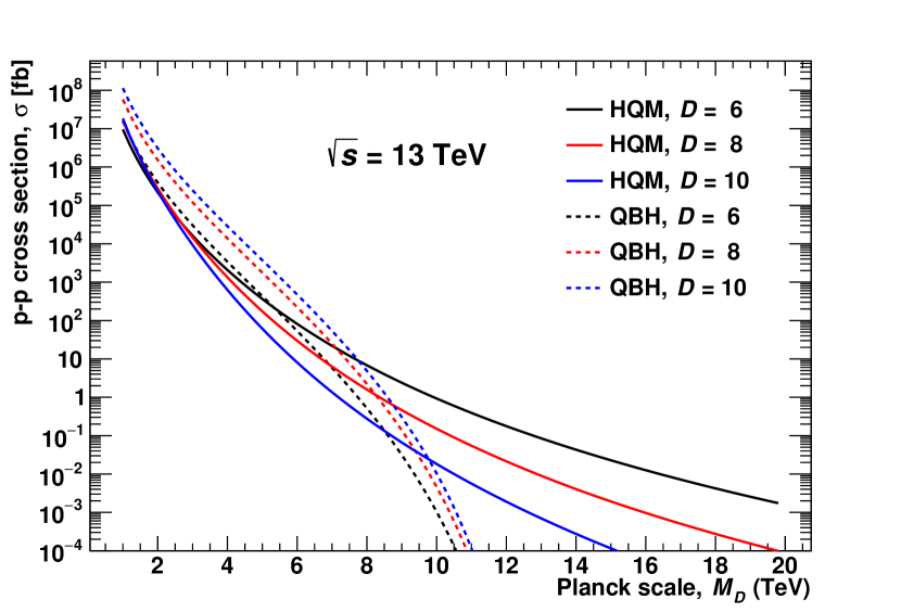
The inclusion of HQM suppresses the total cross section for low $M_{D}$ but predicts a higher cross section than the QBH model at high $M_{D}$. It is also interesting to note how the role of dimensionality is reversed in the two models. For a given $M_{D}$, higher cross sections occur at lower $D$ in the HQM model, except for a small region below about 2 TeV. Also, in the HQM model the cross section at a given $M_{D}$ is significantly different for different $D$ as $M_{D}$ increase. Thus over most of the $M_{D}$ range, dimensionality is significantly more important in the HQM model.

It is also useful to determine the $M_{D}$ value at which the HQM model cross section crosses over the QBH model cross section, and thus where the HQM model might become more significant. For $D=6$, $D=8$, and $D=10$, the crossovers in $M_{D}$ occur at approximately 5.4 TeV, 8.2 TeV, and 9.7 TeV, respectively. To understand which region of $M_{D}$ is interesting, we consider the current lower-limits, at the 95% confidence level, on $M_{D}$ of 9.9 TeV, 6.3 TeV, and 5.3 TeV for $D=6$, $D=8$, and $D=10$, respectively, set by the CMS [35] and ATLAS [36] experiments. At these $M_{D}$ limits, black hole production in the HQM model is still well below the QBH model except for $D=6$ where the HQM model predicts a cross section of about three orders of magnitude higher than the QBH model.

The lower limits on $M_{D}$ are based on graviton searches in the same large extra dimensions paradigm [1, 2] as used for black hole models, and we thus take them to be applicable to both the QBH and HQM models considered here. Searches for QBHs have set limits on $M_{\mathrm{th}}$ (or $M_{D}$ as a function of $M_{\mathrm{th}}$), and thus do not constrain the HQM model; there are currently no limits on $M_{D}$ using the HQM model.

The most glaring difference between models occur above the $M_{D}$ lower limits. While the QBH model cross sections falls sharply as $M_{\mathrm{th}}=M_{D}$ is pushed toward $\sqrt{s}$, the HQM model cross sections exhibit a more gradual drop that becomes less steep at higher $M_{D}$. This results in some notable properties unique to the HQM model. First, black holes may be produced even if $M_{D}>\sqrt{s}$. Second, since the cross sections do not converge to zero at $M_{D}=\sqrt{s}$, dimensionality plays a greater role at high $M_{D}$.

Figure 3: Luminosity required to produce ten black hole events as a function of Planck scale $M_{D}$ at a center of mass energy of 13 TeV. Curves for different models and total number of space-time dimensions $D$ are shown. Solid curves are used for the horizon quantum mechanics (HQM) model and dashed curves are used for the quantum black hole (QBH) model. The horizontal dotted line represents a luminosity of 139 fb^-1.

Of particular importance for observing quantum black holes in experiments is the number of black hole events we are able to produce. Typically, a minimum of ten signal events is sought to form a reasonable claim of discovery In Fig. 3, we plot the luminosity required to produce ten events in proton–proton collisions at $\sqrt{s}=13$ TeV. Analysis performed by ATLAS and CMS using the full run-2 dataset typically quote a luminosity of about 139 fb^-1. Using this luminosity, more than ten events can be produced in the QBH model for $M_{D}$ less than about 8.7 TeV, 9.2 TeV, and 9.5 TeV for $D=6$, $D=8$, and $D=10$, respectively. The lower limits on $M_{D}$ would exclude $D=6$ black holes in the QBH model. The current best lower limit from a direct QBH search is $M_{\mathrm{th}}=M_{D}>9.4$ TeV for $D=10$ [28]. Even with a luminosity of 1 ab^-1 at $\sqrt{s}=13$ TeV, the limit on $M_{\mathrm{th}}$ in the QBH model is unlikely to go above about 10.5 TeV. Thus, the QBH model is being significantly restricted even at current luminosities.

The LHC is able to produce black holes at much higher values of $M_{D}$ in the HQM model for most $D$. At a current luminosity of 139 fb^-1, values of $M_{D}$ in the HQM model are not constrained by the lower limits on $M_{D}$, and quantum black holes could exist in the LHC experiment’s current datasets. However, as we will see next it will be non-trivial to detect HQM black holes in current ATLAS and CMS datasets even if produced.

IV Proton–proton differential cross section

The inclusion of HQM in quantum black hole production has notable implications on the $M$ distribution of black holes. Since the cross sections of QBH and HQM models typically differ by over an order of magnitude (except at very low $M_{D}$ and near the crossing), it is illustrative to compare the normalized shapes of distributions for $M_{D}$ of interest. Figure 4 compares $M$ distributions for four selected values of $M_{D}$ and $D=10$.

For a small $M_{D}$, the HQM model gives the peak structure of the QBH model, but this changes for higher $M_{D}$, and $M$ is distributed over a wide range: $2\lesssim M\lesssim 10$ TeV. This difference in shape is a direct consequence of the shapes of the PDFs and the $P_{\,\mathrm{BH}}$ curve from HQM. The PDFs fall rapidly as parton energies approach $\sqrt{s}/2$. For $M_{D}=12$ TeV in the QBH model, a very small cross section is expected since $M$ is limited to the range $12<M<13$ TeV. In the $M_{D}=12$ TeV HQM model, the lower mass for black holes is dictated by the $P_{\,\mathrm{BH}}$ curve. Black hole masses below 2 TeV are suppressed since $P_{\,\mathrm{BH}}\approx 0$, and likewise black holes with mass above about 10 TeV are suppressed by the PDFs. This interplay in the HQM model between the convolution of PDFs and $P_{\,\mathrm{BH}}$ gives rise to the shape of the $M$ distributions.

Figure 4: Quantum black hole (QBH) model and horizon quantum mechanics (HQM) model mass $M$ distributions normalized to unity for a) $M_{D}=1~{}$TeV, b) $M_{D}=4$ TeV, c) $M_{D}=8$ TeV, and d) $M_{D}=12$ TeV. The center of mass energy is 13 TeV and $D=10$.

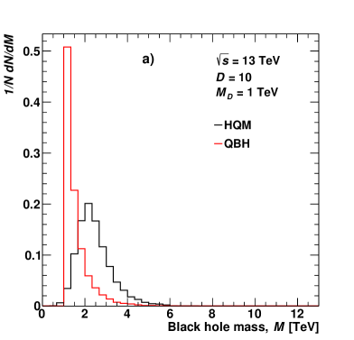
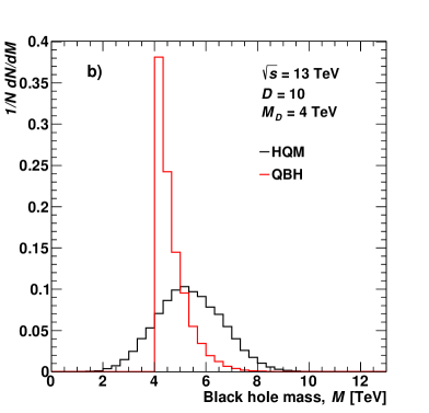
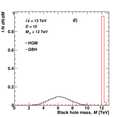
The peak in the QBH $M$ distribution moves up with increasing $M_{D}$ since the model’s definition of $M_{\mathrm{th}}$ is a strict cutoff in $M$. In contrast, the HQM model $M$ distribution does not appear to shift up much above $M_{D}\gtrsim 7$ TeV. This phenomena is explored further in Fig. 5. While the QBH model $M$ distribution moves up with increasing $M_{D}$ acting as a minimum mass threshold, the HQM model $M$ distributions are much more spread out and the shape of the distributions do not change significantly once $M_{D}$ exceeds a few TeV. We also observe that in the HQM model it is very difficult to produce black hole masses above $\sim 11$ TeV, even though $M_{D}$ is not limited.

Figure 5: Quantum black hole (QBH) model a) and horizon quantum mechanics (HQM) model b) proton–proton differential cross sections $d\sigma/dM$ versus black hole mass $M$ for selected values of the Planck scale $M_{D}$. The center of mass energy is 13 TeV and total number of space-time dimensions $D=10$.

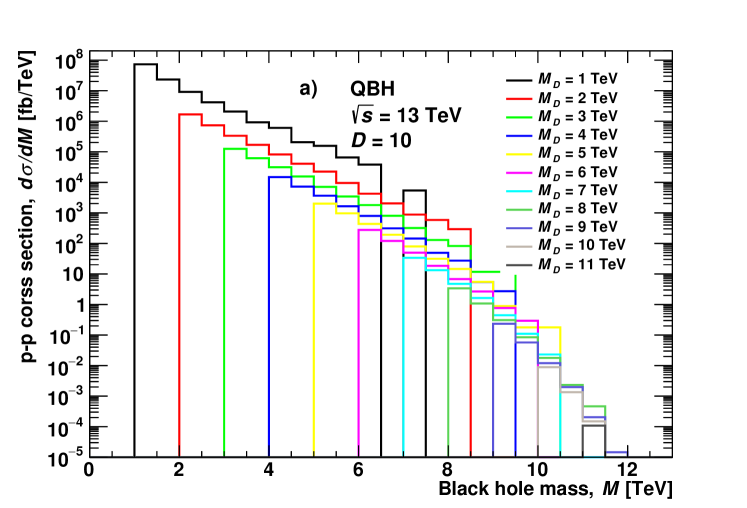
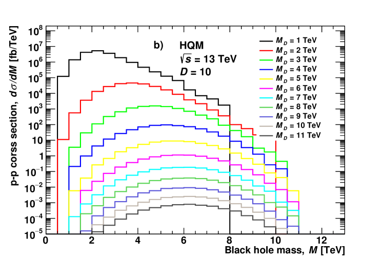
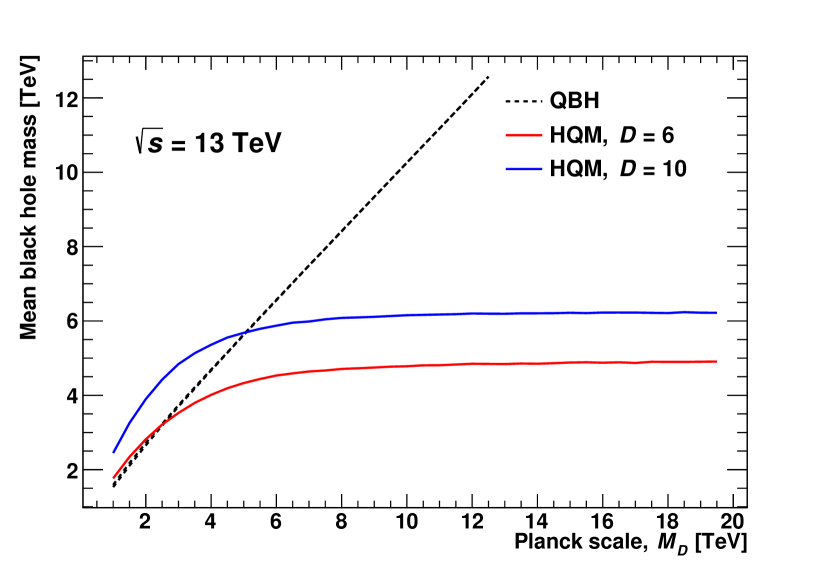
The progression of black hole $M$ distributions with $M_{D}$ in both models is shown in Fig. 6, which plots the mean $M$ as a function of $M_{D}$. The QBH model curve gives exactly what is expected, since most black holes are produced with mass $M_{D}$, a linear increase in the mean $M$ is observed for all $D$. This is in contrast to the HQM model which resembles a linear increase only for small $M_{D}$ and then levels off at a constant mean $M$ for $M_{D}\gtrsim 8$ TeV. The value of the mean $M$ to which the trend converges is dependent on $D$. The reason for this is an interplay between the $P_{\,\mathrm{BH}}$ curves which approach zero as $M$ approaches zero and the PDFs which approach zero as $M$ approaches $\sqrt{s}$. The consequence is a “pinching off” that serves to create a mass distribution that does not change shape significantly between the two mass regions where the production of black holes is vanishingly small. The mean $M$ increases with $D$ due to the $P_{\,\mathrm{BH}}$ curve being shifting higher in $M/M_{D}$ with increasing $D$, as previously shown in Fig. 1.

Figure 6: Mean mass of black hole events as a function of Planck scale $M_{D}$ at a center of mass energy of 13 TeV. Quantum black hole (QBH) and the horizon quantum mechanics (HQM) models are shown for two values of total number of space-time dimensions $D$.

Finally, the shape of the HQM model $M$ distribution has implications on how black holes in this model may be detected in the ATLAS and CMS experiments. In the QBH model, black holes are expected to predominantly decay into two-body final states. The majority of these decay products would be quarks and gluons that would hadronize to produce jets. For this reason, ATLAS and CMS have searched for resonances in the mass distribution of dijet events. The branching fraction to dijets is greater than 96% [23]. The experiments have taken the branching fraction to dijets to be unity and have accounted for events with less than two jets in the efficiency. In our study, we have ignored this inefficiency.

To investigate how black holes in the HQM model would appear in these searches, we use 139 fb^-1 of ATLAS data recorded during run-2 at $\sqrt{s}=13$ TeV [28] . Quantum black hole events are simulated using the same selection criteria, at the particle level, as in the ATLAS analysis. We understand that particle-level selection will only roughly emulate the geometrical acceptance of events in the the ATLAS detector, but the signal yields should be indicative of a full experimental analysis.

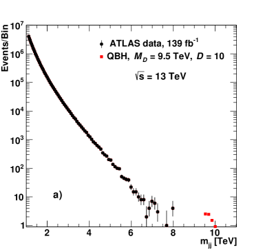
In Fig. 7, the black hole events have been scale by the cross section times luminosity divided by the number of generated events. Fractional events are possible. Figure 7a) shows an example QBH resonance for $M_{D}=9.5$ TeV and $D=10$. This resonance is beyond the highest dijet mass event obtained by ATLAS. In addition, the decisive lack of such a resonance structure in the dijet mass spectrum has allowed ATLAS to limit black holes in the QBH model to $M_{\mathrm{th}}>9.4$ TeV for $D=10$ at the 95% confidence level [28]. Thus, the QBH model in its simplest form is close to being ruled out.

Figure 7: Black hole dijet mass distributions scaled by cross section to the ATLAS data luminosity and added on top of the ATLAS dijet mass m_jj spectrum measured at a center of mass energy of 13 TeV and a luminosity of 139 fb^-1 [28]. The results are shown for the quantum black hole (QBH) model and horizon quantum mechanics (HQM) model for various values of the Planck scale $M_{D}$ and the total number of extra space-time dimensions $D$.

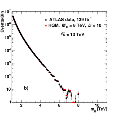
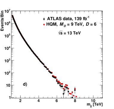
For the HQM model, dijet distributions are shown in Fig. 7b), Fig. 7c), and Fig. 7d) for ($M_{D}=8$ TeV, $D=10$), ($M_{D}=8.5$ TeV, $D=8$), and ($M_{D}=9$ TeV, $D=6$), respectively. Although ATLAS and CMS have not set limits on the HQM model they have eliminated a wide variety of resonances in the dijet mass spectrum from trigger turn on to about 8 TeV. Thus HQM black hole production resulting in sizable deviations from the smoothly falling dijet mass distribution are not allowed. The values of $M_{D}$ in the figures have been chosen high enough to not result in a clear enhancement in the dijet mass distribution that ATLAS and CMS have not seen. On the other hand, if the $M_{D}$ values are chosen higher the number of events becomes insignificant for masses above the ATLAS and CMS data points. It would thus be extremely difficult to observe black holes in the HQM model in the current dijet invariant mass spectrum.

V Discovery potential in the dijet mass distribution

In order to predict the discovery potential for observing quantum black holes, we take into consideration both the number of events above background and the significance of the signal. For the significance, we use the asymptotic approximation without background uncertainty (see, for example Ref. [40]). The formula comes from using the asymptotic formulae for the distributions of profile likelihood test statistics.

$$\sigma=\sqrt{2\left[\left(s+b\right)\ln\left(1+\frac{s}{b}\right)-s\right]}\,,$$ (4)

where $s$ is the number of signal events above background and $b$ is the number of background events excluding signal events. The signal events are generated with Qbh and the ATLAS background model is taken as the background. We understand that Eq. (4) is an approximation based on a cut-and-count approach, and that one should really include background uncertainties. However, such an analysis is beyond the scope of this work, and is unlikely to change the qualitative findings.

We consider a significant observation to be greater than $5\sigma$. Using a cut-and-count method, significance is calculated by counting events above $M_{\mathrm{th}}$. While this is natural for the QBH model, it is perhaps not so meaningful for the HQM model since many of the events have $M<M_{D}$. For the sake of comparison, we consider two approaches to calculating the significance for the HQM model. The first is the usual definition, where we consider $M_{D}$ as a cutoff. In this method $M_{D}$ values beyond $\sqrt{s}$ can not be probed. In the second method, we consider all black hole events and count the background from the least massive signal event. We understand that the latter method would be extremely difficult, and probably not even desirable, to realize in an experiment’s analysis, but it might be more indicative of a shape-fit procedure that might likely be used.

The event count and significance are presented in Fig. 8 and Fig. 9, respectively. While counting HQM model events over the entire mass range gives the greater number of events, the method of counting HQM model events only above $M_{D}$ give better significances. This could have been anticipated given the large number of background events at low dijet masses. Using either approach to calculating the significance, the discovery potential at allowed values $M_{D}$ is less for the HQM model than the QBH model. Since the ATLAS background that we are using does not extend beyond 8.1 TeV, and because of the simple significance formula Eq. (4), the significance curves in Fig. 9 end at $M_{D}=8$ TeV.

Figure 8: Predicted number of black hole events versus Planck scale $M_{D}$ for a center of mass energy of 13 TeV and luminosity of 139 fb^-1 when selecting events at the parton level according to the same criteria as the search in Ref. [28]. The solid curves are for total space-time dimension $D=10$ and the dashed curves for $D=6$.

Figure 9: Significance of a black hole observation above dijet background versus Planck scale $M_{D}$ for a center of mass energy of 13 TeV and luminosity of 139 fb^-1. Event were selected at the parton level according to the same criteria as the search in Ref. [28]. The solid curves are for total space-time dimension $D=10$ and the dashed curves for $D=6$.

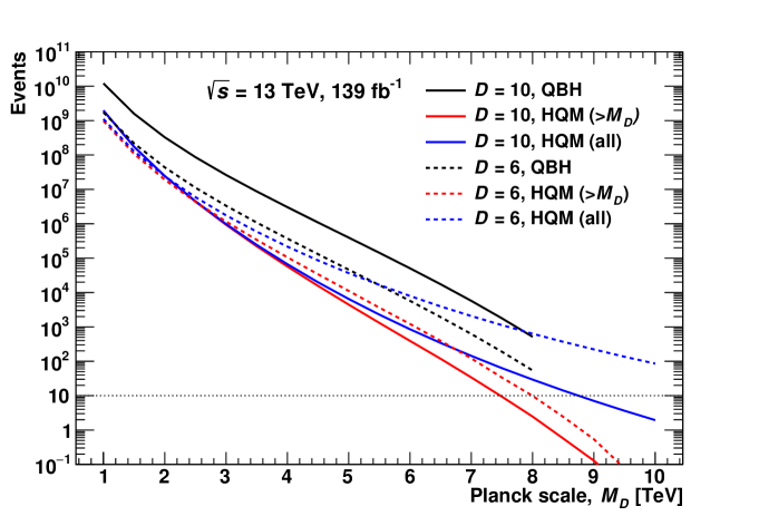
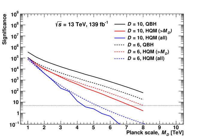
Using the $M>M_{D}$ counting method and by noting the minimum $M_{D}$ value given by the ten event and $5\sigma$ criteria, we assess the possibility of detecting HQM black holes in ATLAS and CMS. For $D=10$, the number of signal events is greater than ten for $M_{D}\lesssim 7.5$ TeV. The corresponding significance is greater than $5\sigma$ for $M_{D}\lesssim 7.4$ TeV, and this sets the upper limit on $M_{D}$ to observe black holes in the HQM model. For the $D=6$ case, greater than ten events occurs when $M_{D}\lesssim 8.0$ TeV and the significance is greater than $5\sigma$ at $M_{D}\lesssim 8.0$ TeV. However, with only one background event, the significance as defined in Eq. (4) slightly overestimates the true significance. In any case, the lower limit on $M_{D}$ from the CMS experiment [35] for $D=6$ is 9.9 TeV at the 95% confidence level, thus eliminating the HQM model for $D=6$.

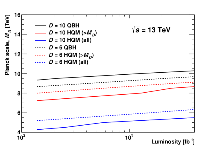
Given the increase in luminosity and $\sqrt{s}$ in subsequent LHC runs, these discovery potentials stand to increase somewhat. With this thought in mind, we make some predictions at $\sqrt{s}=13$ TeV on the luminosity required at a given $M_{D}$ for a meaningful discovery. We assume that the number of background events, based on the background model from Ref. [28], scales linearly with luminosity. When calculating the significance using $M>M_{D}$ as a cutoff in the cut-and-count method, we have made the additional assumption that event-count is the limiting factor for $M_{D}>8$ TeV as this is the highest dijet mass at which the ATLAS background estimate is given. The results are shown in Fig. 10 where we only consider luminosities above 139 fb^-1. The luminosity axis of the plot extends out to 4000 fb^-1, inspired by the design integrated luminosity of the High-Luminosity Large Hadron Collider. It is seen that the increase in probing $M_{D}$ with a reasonable increase in luminosity is not very significant, indicating that we are close to exhausting the search for black holes in both QBH and HQM models using the dijet mass distribution at $\sqrt{s}=13$ TeV. Although we have used a very simplistic approach to estimating the discovery potential, this conclusion is unlikely to change with a more robust estimate.

Figure 10: Minimum luminosity required to produced at least ten signal events and a significance of $5\sigma$ at a center of mass energy of 13 TeV. The solid curves are for total space-time dimension $D=10$ and the dashed curves for $D=6$.

VI Conclusions

Microscopic black hole formation as predicted by HQM was implemented in the Qbh MC event generator to investigate the impact on possible black hole production at the LHC. The inclusion of the HQM model serves to decrease the total black hole cross section for small $M_{D}$, but the new model is not restricted by a threshold mass requirement. Therefore, HQM predicts black holes may be produced at $M_{D}\sim\sqrt{s}$. The HQM model is also highly dependent on dimensionality and predicts that a greater number of events may be produced with a smaller $D$. The $M$ distribution is also greatly affected by HQM with a much wider spread of black hole masses. In other words, there is no resonance structure in the HQM model. This wide $M$ distribution converges to a constant shape for large $M_{D}$, which can be considered to be one of the defining features of the HQM model.

The predicted signal in the dijet mass distribution along with the ATLAS run-2 background model were used to estimate the number of signal events and significance. Observations of quantum black holes governed by HQM were predicted to be limited to $M_{D}\lesssim 8.0$ TeV for $D=6$ and $M_{D}\lesssim 7.2$ TeV for $D=10$.

Given the small potential for observation of HQM black holes in the dijet mass distribution, a discovery in the invariant mass variable is unlikely. Alternatively, an angular search may be performed to distinguish an enhancement of events due to black hole production above QCD background [12, 13, 21, 23, 24]. The HQM model does not yet predict any modification to the usual decays in the QBH model; there is no difference between the two models in terms of the shape of angular distributions.

An example angular search could be in the variable $\chi$ defined as

$$\chi=e^{|y_{1}-y_{2}|}\,,$$ (5)

where $y_{1}$ and $y_{2}$ are the rapidities of the two jets. QCD $t$-channel scattering constituting the background is approximately constant in $\chi$, while $s$-channel resonances tend to be enhanced at low $\chi$. Because of this, an angular search could help uncover the wide $s$-channel mass enhancement that is predicted by HQM. Since the predictions of an angular search are highly dependent on the analysis and detector details, we leave it to the ATLAS and CMS collaborations to perform such a search.

Some of the above results were first mentioned in Ref. [11]. Unfortunately, that paper could only make use of ATLAS and CMS results from about 20 fb^-1 of data at a center of mass energy of 8 TeV. We view our analysis as more comprehensive, benefiting from using recently available experimental data distributions, and up to date.

Lastly, although the HQM model has been used, we do not believe the qualitative results presented here depend specifically on the formula presented in Ref. [9]; similar results would be obtained for any non-step-like threshold mass production of black holes such as those presented in Ref. [10].

We have implemented and studied a benchmark model and some of the quantitative results are model dependent. It is not our intent to prove or disprove a particular model but to point out the need for alternative search strategies for quantum black holes such as a dijet angular analysis.

Appendix A Monte Carlo event generation

In order to visualise how the HQM probability $P_{\,\mathrm{BH}}$ varies with $D$, $M_{D}$, and $M$, we computed the integral in Eq. (2) explicitly using numerical integration. As shown in Fig. 1, good accuracy was achieved with the use of Simpson’s method and an adequate large number of subdivisions.

A more elegant means of producing the appropriate $P_{\,\mathrm{BH}}$ factor can be performed by MC integration. As a check, we have also produced the curves in Fig. 1 using MC sampling. By integrating and inverting the $\mathcal{P}_{\,\mathrm{H}}$ distribution, random values of the horizon radius $r_{\mathrm{H}}$ can be sampled using a uniform distribution of random numbers. Since $\mathcal{P}_{\,\mathrm{H}}$ is a probability density function, using random $r_{\mathrm{H}}$ values to calculate $P_{\,\mathrm{S}}$ for a large number of samples effectively computes the expected value for $P_{\,\mathrm{S}}$ (or equivalently, $P_{\,\mathrm{BH}}$). For completeness, we present this calculation.

We begin from Eq 3.7 in Ref. [9]:

$$\mathcal{P}_{\,\mathrm{H}}(r_{\mathrm{H}}) = a^{\frac{d}{d-2}}\frac{2(d-2)}{\Gamma\left(s,1\right)}\Theta(r_{\mathrm{H}}-R_{d})$$ (6)

$$\times\exp\left(-a^{2}r_{\mathrm{H}}^{2(d-2)}\right)r_{\mathrm{H}}^{d-1}\,,$$

where in this appendix we use the notion of Ref. [9] except we take the total number of spatial dimensions to be $d$. We have define $a=(d-2)/(2m)$ and $s=d/[2(d-2)]$, and used $\Delta=m$ as in Ref [9]; $\Gamma(s,x)=\int_{x}^{\infty}t^{s-1}e^{-t}dt$ is the upper incomplete Gamma function. In addition, we are using Planck units since we are only interested in lengths and masses relative to $M_{D}$.

By taking the Heaviside step function to be one, the indefinite integral can be computed:

$$\int\mathcal{P}_{\,\mathrm{H}}(r_{\mathrm{H}})dr_{\mathrm{H}}=-\frac{\Gamma\left(s,a^{2}r_{\mathrm{H}}^{2(d-2)}\right)}{\Gamma\left(s,1\right)}\,.$$ (7)

Substituting a lower limit of $R_{d}=[2m/(d-2)]^{1/(d-2)}$ and upper limit of $r_{\mathrm{H}}$, to allow calculation of the cumulative distribution function, gives

$$\mathrm{CDF}[\mathcal{P}_{\,\mathrm{H}}(r_{\mathrm{H}})]=1-\frac{\Gamma\left(s,a^{2}r_{\mathrm{H}}^{2(d-2)}\right)}{\Gamma\left(s,1\right)}\,.$$ (8)

If we generate a uniform random real number $u$ in the interval $(0,1)$ [or $1-u$ in the interval $(1,0)$] and set it equal to Eq. (8), we can solve for $r_{\mathrm{H}}$ by inverting the incomplete Gamma function with respect to its second parameter:

$$r_{\mathrm{H}}=R_{d}\left[Q^{-1}\left(s,Q(s,1)u\right)\right]^{\frac{1}{2(d-2)}}\,.$$ (9)

Note that $Q^{-1}(s,Q(s,x))=x$, where $Q^{-1}$ is the inverse of the regularized upper incomplete Gamma function $Q(s,x)=\Gamma(s,x)/\Gamma(s)$. There are numerical methods to optimise this inversion.

Upon randomly sampling the horizon radii from Eq. (9), we return values of $P_{\,\mathrm{S}}(r<r_{\mathrm{H}})$ as given by Eq. 3.5 in Ref. [9]:

$$P_{\,\mathrm{S}}(r<r_{\mathrm{H}})=\frac{\gamma\left(\frac{d}{2},m^{2}r_{\mathrm{H}}^{2}\right)}{\Gamma\left(\frac{d}{2}\right)}\,,$$ (10)

where $\gamma(s,x)=\int_{0}^{x}t^{s-1}e^{-t}dt$ is the lower incomplete Gamma function.

The above random horizon generation can simply be looped over with an average of all $P_{\,\mathrm{S}}$ values giving an approximate value for $P_{\,\mathrm{BH}}$. We easily recreate the same probability curves as in Fig. 1 which used Simpson’s method.

Both the MC method and Simpson’s method for calculating $P_{\,\mathrm{BH}}$ have been implemented in Qbh. Despite both methods producing the same results, there are technical pros and cons of each method. The MC HQM calculation just presented is the default method.

One additional technicality should be mentioned. Since black hole production in the HQM model allows for $M$ less than $M_{D}$ there is no lower-mass cutoff in the generator. Instead, the $P_{\,\mathrm{BH}}$ curve imposes its own smooth limit as it becomes arbitrarily small. To sample $M$ via a power transformation of the cross section used to increase efficiency, we choose an arbitrary minimum of 100 GeV since in practise it is exceedingly rare to generate an event with $M$ this low. For example, selecting a 200 GeV minimum has a negligible impact on the results.

We point out that our curves of $P_{\,\mathrm{BH}}$ are identical to the corresponding figure in Ref. [11] within our ability to read values from their figure. Equation (7) in Ref. [11] disagrees with Eq. (3.8) Ref. [9], although the later cites the former. We believe Eq. (7) in Ref. [11] has the inverse power of $(m_{d}/m)$ and a normalization difference of $(D-2)^{2}$. If the formula in the paper was actually use to generate the plot, the curves continue to increase above unity with increasing mass and do not represent probability distributions.

References

- Arkani-Hamed et al. [1998] N. Arkani-Hamed, S. Dimopoulos, and G. R. Dvali, Phys. Lett. B429, 263 (1998), arXiv:hep-ph/9803315 [hep-ph] .
- Antoniadis et al. [1998] I. Antoniadis, N. Arkani-Hamed, S. Dimopoulos, and G. R. Dvali, Phys. Lett. B436, 257 (1998), arXiv:hep-ph/9804398 [hep-ph] .
- Randall and Sundrum [1999] L. Randall and R. Sundrum, Phys. Rev. Lett. 83, 3370 (1999), arXiv:hep-ph/9905221 [hep-ph] .
- Giddings and Thomas [2002] S. B. Giddings and S. D. Thomas, Phys. Rev. D65, 056010 (2002), arXiv:hep-ph/0106219 [hep-ph] .
- Dimopoulos and Landsberg [2001] S. Dimopoulos and G. L. Landsberg, Phys. Rev. Lett. 87, 161602 (2001), arXiv:hep-ph/0106295 [hep-ph] .
- Myers and Perry [1986] R. C. Myers and M. J. Perry, Ann. Phys. (N.Y.) 172, 304 (1986).
- Gingrich [2006] D. M. Gingrich, Int. J. Mod. Phys. A21, 6653 (2006), arXiv:hep-ph/0609055 [hep-ph] .
- Casadio [2015] R. Casadio, Eur. Phys. J. C75, 160 (2015), arXiv:1411.5848 [gr-qc] .
- Casadio et al. [2016] R. Casadio, R. T. Cavalcanti, A. Giugno, and J. Mureika, Phys. Lett. B760, 36 (2016), arXiv:1509.09317 [gr-qc] .
- Mureika et al. [2012] J. Mureika, P. Nicolini, and E. Spallucci, Phys. Rev. D 85, 106007 (2012), arXiv:1111.5830 [hep-ph] .
- Arsene et al. [2016] N. Arsene, R. Casadio, and O. Micu, Eur. Phys. J. C76, 384 (2016), arXiv:1606.07323 [hep-ph] .
- Aad et al. [2011] G. Aad et al. (ATLAS), New J. Phys. 13, 053044 (2011), arXiv:1103.3864 [hep-ex] .
- Aad et al. [2013] G. Aad et al. (ATLAS), JHEP 01 (029), arXiv:1210.1718 [hep-ex] .
- Chatrchyan et al. [2013] S. Chatrchyan et al. (CMS), JHEP 01 (013), arXiv:1210.2387 [hep-ex] .
- Aad et al. [2014a] G. Aad et al. (ATLAS), Phys. Lett. B728, 562 (2014a), arXiv:1309.3230 [hep-ex] .
- Aad et al. [2014b] G. Aad et al. (ATLAS), Phys. Rev. Lett. 112, 091804 (2014b), arXiv:1311.2006 [hep-ex] .
- Aad et al. [2014c] G. Aad et al. (ATLAS), Phys. Rev. D90, 052005 (2014c), arXiv:1405.4123 [hep-ex] .
- Aad et al. [2015] G. Aad et al. (ATLAS), Phys. Rev. D91, 052007 (2015), arXiv:1407.1376 [hep-ex] .
- Khachatryan et al. [2015] V. Khachatryan et al. (CMS), Phys. Rev. D91, 052009 (2015), arXiv:1501.04198 [hep-ex] .
- Khachatryan et al. [2016] V. Khachatryan et al. (CMS), Eur. Phys. J. C 76, 317 (2016), arXiv:1604.05239 [hep-ex] .
- Aad et al. [2016] G. Aad et al. (ATLAS), Phys. Lett. B754, 302 (2016), arXiv:1512.01530 [hep-ex] .
- Aaboud et al. [2016] M. Aaboud et al. (ATLAS), Eur. Phys. J. C76, 541 (2016), arXiv:1607.08079 [hep-ex] .
- Aaboud et al. [2017] M. Aaboud et al. (ATLAS), Phys. Rev. D96, 052004 (2017), arXiv:1703.09127 [hep-ex] .
- Sirunyan et al. [2017] A. M. Sirunyan et al. (CMS), JHEP 07 (013), arXiv:1703.09986 [hep-ex] .
- Aaboud et al. [2018a] M. Aaboud et al. (ATLAS), Eur. Phys. J. C 78, 102 (2018a), arXiv:1709.10440 [hep-ex] .
- Sirunyan et al. [2018a] A. M. Sirunyan et al. (CMS), JHEP 04 (073), arXiv:1802.01122 [hep-ex] .
- Aaboud et al. [2018b] M. Aaboud et al. (ATLAS), Phys. Rev. D 98, 092008 (2018b), arXiv:1807.06573 [hep-ex] .
- Aad et al. [2020] G. Aad et al. (ATLAS), JHEP 03 (145), arXiv:1910.08447 [hep-ex] .
- Note [1] We use QBH to refer to the quantum black hole model and Qbh to refer to the quantum black hole generator of the same name.
- Gingrich [2010a] D. M. Gingrich, Comput. Phys. Commun. 181, 1917 (2010a), arXiv:0911.5370 [hep-ph] .
- Meade and Randall [2008] P. Meade and L. Randall, JHEP 05 (003), arXiv:0708.3017 [hep-ph] .
- Calmet et al. [2008] X. Calmet, W. Gong, and S. D. H. Hsu, Phys. Lett. B668, 20 (2008), arXiv:0806.4605 [hep-ph] .
- Gingrich [2010b] D. M. Gingrich, J. Phys. G37, 105008 (2010b), arXiv:0912.0826 [hep-ph] .
- Pumplin et al. [2002] J. Pumplin, D. R. Stump, J. Huston, H. L. Lai, P. M. Nadolsky, and W. K. Tung, JHEP 07 (012), arXiv:hep-ph/0201195 [hep-ph] .
- Sirunyan et al. [2018b] A. M. Sirunyan et al. (CMS), Phys. Rev. D97, 092005 (2018b), arXiv:1712.02345 [hep-ex] .
- Aaboud et al. [2018c] M. Aaboud et al. (ATLAS), JHEP 01 (126), arXiv:1711.03301 [hep-ex] .
- Note [2] At this point, we are assuming a perfect search for black holes.
- Note [3] The data is taken from the HEPData repository https://www.hepdata.net/record/ins1759712.
- Note [4] The quantum black holes we consider are only effected by the rapidity requirements; the simulated events pass the transverse momentum, invariant mass, and azimuthal angle requirements.
- Cowan et al. [2011] G. Cowan, K. Cranmer, E. Gross, and O. Vitells, Eur. Phys. J. C 71, 1554 (2011), [Erratum: Eur.Phys.J.C 73, 2501 (2013)], arXiv:1007.1727 [physics.data-an] .