Arctic Amplification of Anthropogenic Forcing:
A Vector Autoregressive Analysis

Abstract

On September 15${}^{\text{th}}$ 2020, Arctic sea ice extent (SIE) ranked second-to-lowest in history and keeps trending downward. The understanding of how feedback loops amplify the effects of external $CO_{2}$ forcing is still limited. We propose the VARCTIC, which is a Vector Autoregression (VAR) designed to capture and extrapolate Arctic feedback loops. VARs are dynamic simultaneous systems of equations, routinely estimated to predict and understand the interactions of multiple macroeconomic time series. The VARCTIC is a parsimonious compromise between full-blown climate models and purely statistical approaches that usually offer little explanation of the underlying mechanism. Our completely unconditional forecast has SIE hitting 0 in September by the 2060’s. Impulse response functions reveal that anthropogenic $CO_{2}$ emission shocks have an unusually durable effect on SIE – a property shared by no other shock. We find Albedo- and Thickness-based feedbacks to be the main amplification channels through which $CO_{2}$ anomalies impact SIE in the short/medium run. Further, conditional forecast analyses reveal that the future path of SIE crucially depends on the evolution of $CO_{2}$ emissions, with outcomes ranging from recovering SIE to it reaching 0 in the 2050’s. Finally, Albedo and Thickness feedbacks are shown to play an important role in accelerating the speed at which predicted SIE is heading towards 0.

1 Introduction

With 3.74 million square kilometers on September 15${}^{\text{th}}$ 2020, Arctic sea ice extent ranked second-to-lowest in history, after the record minimum in 2012. A persistent retreat of SIE may further accelerate global warming and threaten the composition of the Arctic’s ecosystem (ScSim10). The Coupled Model Intercomparison Project (CMIP) assembles estimates of long-run projections of Arctic sea ice from many climate models. These models try to reproduce the geophysical dynamics and interrelations among various variables, influencing the evolution of global climate.

With CMIP being in its 6${}^{\text{th}}$ phase (CMIP6), climate models now provide more realistic forecasts of the Arctic’s sea ice cover compared to its predecessor CMIP5 (see StroeveEtAl12, Notzetal2020). The majority of contributors to CMIP6 see the Arctic’s September mean sea ice to retreat below the $1\times 10^{6}$ $km^{2}$ mark before the year 2050. Despite following the hitherto accepted physical laws of our climate, its chaotic nature, i.e. the still obscure interplay of various climate variables, imposes a major burden on climate models. Repeated initialization with differing starting conditions is intended to reduce uncertainty and biases surrounding initial parameters. The byproduct is a wide range of projections of key climate variables (Notzetal2020). In addition to such tuning, these simulations require large amounts of input data and a coupling of various sub-models (TaylorEtAl09).

The above raises the question whether an approach that is statistical and yet multivariate can paint a more conciliating picture. This means estimating a statistical system that depicts the interaction of key variables describing the state of the Arctic. In such a setup, the downward SIE path will be an implication of a complete dynamic system based on the observed climate record. We provide a formal statistical assessment of different hypotheses about the historical path of SIE and outline the implications for the future. The effects on Arctic sea ice arising from various physical processes – and the uncertainty surrounding their estimation – can both be quantified without resorting to use a climate model.

Feedback Loops. Feedbacks are dynamics initially triggered by an external shock to the system. Such a disturbance can be of radiative nature or not. Our analysis aims at better understanding how feedback loops – and their interaction with anthropogenic carbon dioxide ($CO_{2}$) forcing – shape the response of key Arctic variables, and most notably, sea ice. $CO_{2}$ forcing is already widely suspected to be the main driver behind long-run SIE evolution (see Meier2014, notz2017arctic). Feedback loops are well documented in the literature (see Park13, Winton13, StueEtAl18, McGraw19) and their understanding is crucial for enhancing the predictability of the Arctic’s sea ice cover (Wang16, Notzetal2020). Only an approach that considers the interaction of many variables in a flexible way – and thus numerous potential sources for feedback loops – has a chance to depict a reliable statistical portrait of the Arctic. CMIP6 models consider many variables, but high variation in sea ice projections (see Notzetal2020) suggests (among other things) widespread uncertainty around how strongly feedback loops may amplify external forcing. To shed more compelling statistical light on the matter, we borrow a methodology from economics.

The Varctic. Our analysis focuses on the evolution of the long-term trajectory of SIE and the interdependent processes behind it. The modeling approach, which we propose, achieves a desirable balance between purely statistical and theoretical/structural approaches. In many fields, statistical approaches often have a better forecasting record than theory-based models. An obvious drawback is that the successful statistical model may provide little to no explanation of the underlying physical processes.

A Vector Autoregression (VAR) lives in a useful middle ground. It is a statistical model that yet generates forecasts by iterating a complete system of difference equations in multiple endogenous variables. These interactions can be analyzed and provide an explanation for the resulting forecasts. Considering all this, we propose the VAR for the Arctic (VARCTIC), a statistical approach that (i) can generate long-run forecasts, (ii) can explain them as the result of feedback loops and external forcing (iii) allows us to analyze how the Arctic responds to exogenous impulses/anomalies.

Roadmap. We first discuss the data and its transformation in section 2. We proceed with discussing the VAR model, its identification and Bayesian estimation in section 3. Section 4 contains the empirical results which comprise (i) a long-run forecast of SIE, (ii) impulse response functions of the VAR, (iii) an exploration of the transmission mechanism (feedback loops), and (iv) a conditional forecasting analysis. We conclude and propose directions for future research in section 5.

2 Data

Our data set comprises eighteen time series, proxying the Arctic’s climate system, and accounting for potential feedback loops among the different constituents. The sample covers monthly observations from 1980 through 2018. We rely on standard data providers (see stroeve2018), which are listed in Table 1 in the appendix. We combine eight variables, which importance has been highlighted by the existing literature (Meier2014), into VARCTIC 8, our benchmark specification. Fortunately, variables can easily be added/removed from a VAR. Bayesian shrinkage ensures that a larger model will not overfit – the latter aspect is further explained in section 3.5. Therefore, the appendix contains VARCTIC 18 which includes an additional 10 series from the reanalysis product MERRA2 (MERRA2) as a robustness check. To summarize compactly, the two specifications considered in this paper are:

• VARCTIC 8: $CO_{2}$, Total Cloud Cover (TCC), Precipitation Rate (PR), Air Temperature (AT), Sea Surface Temperature (SST), Sea Ice Extent (SIE), Sea Ice Thickness (SIT), Albedo;

• VARCTIC 18: SWGNT, SWTNT, $CO_{2}$, LWGNT, TCC, TAUTOT, PR, TS, AT, SST, LWGAB, LWTUP, LWGEM, SIE, Age, SIT, EMIS, Albedo.

A comprehensive overview of all variables (including those of VARCTIC 18), their acronyms, and links to data providers can be found in the appendix in Table 1. We want the VARCTIC to be a credible approximation of a completely endogenous system, where local processes jointly determine each other, without significant external dependencies outside of forcing. Thus, we restrict the spatial coverage to a regional rather than a global scale. In line with the literature (notz2016observed), all variables (except $CO_{2}$, which is measured globally, and SST, which is measured over the Northern Hemisphere (HorvathEtAl2020)) are monthly means over all grid-cells between 30^∘N and 90^∘N latitude. This region matches the spatial coverage of the Sea Ice Index and is in the neighborhood of the lower bound of 40^∘N latitude applied in HorvathEtAl2020. It is a legitimate concern that averaging over too large of a region could wrongfully blend together mid-latitude events with others more specific to the Arctic circle. Fortunately, all key findings remain unchanged when restricting the gridded variables of TCC, PR, AT, and Albedo to the 60^∘N-90^∘N domain. An interesting avenue for future research is to consider a (larger) VAR where means over various latitude ranges are included – so to study their interactions and relationship with SIE. Further, we follow OelkeEtAl2003 and use AT measured at a sigma-level of 0.995, i.e. at 0.995 $times$ each grid-cell’s surface-level pressure. For its part, the important choice of VARCTIC 8’s variables themselves (and additions in VARCTIC 18) will be motivated extensively in section 3.3.

The raw data is highly seasonal — but the feedback loops we wish to estimate and extrapolate, reside in the (stochastic) trend components and short-run anomalies. Hence, we proceed to transform the data so that the resulting VARCTIC is fitted on deviations from seasonal means. For our benchmark analysis, we use a simple and transparent transformation: we de-seasonalize our data by regressing a particular variable $y^{raw}$ on a set of monthly dummies. That is, for each variable we run the regression

$$y_{t}^{raw}=\sum_{m=1}^{12}\alpha_{m}D_{m}+\text{residual}_{t}$$ (1)

with $y_{t}$ being defined as $y_{t}\equiv y_{t}^{raw}-\sum_{m=1}^{12}\hat{\alpha}_{m}D_{m}$. $D_{m}$ is an indicator that is 1 if date $t$ is in month $m$ and 0 otherwise. The estimates of $\alpha_{m}$, $\hat{\alpha}_{m}$, are obtained by ordinary least squares. This is exactly equivalent to de-meaning each data series month by month and is a more flexible approach to modeling seasonality than using Fourier series. Finally, we keep our filtered data $y$ in levels. We do not want to employ first differences or growth rate transformations to make the data stationary. Such an action would suppress long-run relationships which are an important object of interest. Figure 1 in the Appendix shows the data after being filtered with monthly dummies.

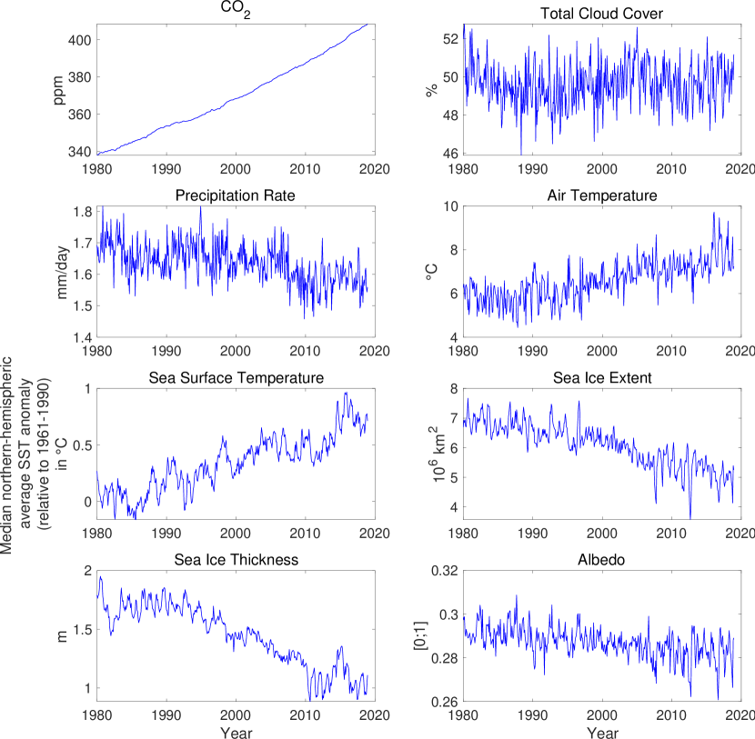
Figure 1: Deseasonalized Series: 8 Variables

Pre-processing the data can influence results. Moreover, DieRu19 and Meier2014 document seasonal variability in SIE trends. As a natural robustness check, we also consider a very different approach to eliminate seasonality. In appendix A.6, we reproduce our results with a data set of stochastically de-seasonalized variables obtained from the approach of structural time series (Harvey90 and harvey2014). In short, this extension allows for seasonality to evolve (slowly) over time, which could be a feature of some Arctic time series.

3 The VARCTIC

In this section, we review the VAR: the model; its identification; its Bayesian estimation. Furthermore, we discuss the construction of the long-run forecasts and impulse response functions as tools to understand the VARCTICs’ results.

3.1 Vector Autoregressions and Climate

Vector Autoregressions are dynamic simultaneous systems of equations. They can characterize a linear dynamic system in discrete time. The methodology was introduced to macroeconomics by sims1980 and is now so widely used that it almost became a field of its own (see kilian2017svar). It is a multivariate model in the sense that $\bm{y}_{t}$ in

$$A\bm{y}_{t}=\Psi_{0}+\sum_{p=1}^{P}{\Psi_{p}}\bm{y}_{t-p}+\bm{\varepsilon}_{t},$$ (2)

is an $M$ by 1 vector. This means that the dynamic system incorporates $M$ variables. $\Psi_{p}$’s parameterizes how each of these variables is predicted by its own lags and lags of the $M-1$ remaining variables. The matrix $A$ characterizes how the $M$ different variables interact contemporaneously — e.g., how AT affects SIE within the same month (a time unit $t$ in our setup). Finally, the disturbances are mutually uncorrelated with mean zero:

$$\bm{\varepsilon}_{t}=\left[\varepsilon_{1,t},\enskip...\enskip,\varepsilon_{M,t}\right]\leavevmode\nobreak\ \sim\leavevmode\nobreak\ \,N\left(0,\leavevmode\nobreak\ I_{M}\right).$$

Equation (2) is the so-called structural form of the VAR, which cannot be estimated because $A$ is not identified by the data. For clarity, the elements of $A$ are not plain regression coefficients, but structural model parameters. Attempting to estimate those directly via least squares would be plagued by simultaneity bias (kilian2017svar). Rather, structural VAR estimation proceeds in two steps. First, an estimable "reduced-form" VAR is fitted to the data. That is, we run

$$\bm{y}_{t}=\bm{c}+\sum_{p=1}^{P}{\Phi_{p}}\bm{y}_{t-p}+\bm{u}_{t},$$ (3)

where $\bm{c}=A^{-1}\Psi_{0}$ and $\Phi_{p}=A^{-1}\Psi_{p}$ are both regression coefficients. $\bm{u}_{t}$ are now regression residuals

$$\bm{u}_{t}=\left[u_{1,t},\enskip...\enskip,u_{M,t}\right]\leavevmode\nobreak\ \sim\leavevmode\nobreak\ \,N\left(0,\leavevmode\nobreak\ \Sigma_{u}\right)$$

which are allowed to be cross-correlated. By construction, $\Sigma_{u}=A^{-1^{\prime}}A^{-1}$. This last relationship is key to the second, so-called "identification", step. In words, this means the covariance matrix of regression residuals from the first step ($\Sigma_{u}$) can be used as raw material to retrieve the "structural" $A$ — the latter which, as we stressed earlier, cannot be estimated directly. The process for obtaining $A$ by decomposing $\Sigma_{u}$ is addressed on its own in section 3.3.

The methodology has many advantages over simple autoregressive distributed lags (ARDL) regression that have gained some popularity in the econometric and climate literature. For instance, in mcgrawbarnes2018, the argument for inclusion of lags of the dependent variable can be interpreted as one for completeness of the modeled dynamic system, as guaranteed by an adequately specified VAR.

3.2 Obtaining Long-Run Forecasts from a VAR

The symmetry of the VAR allows for it to generate forecasts by simply iterating the model. Assuming the chosen variables to characterize the system completely, we can forecast its future state by iterating a particular mapping. To do so, we use a representation that exploits the fact that any VAR($P$) (that is, with $P$ lags) can be rewritten as a VAR(1), using the so-called companion matrix. Thus, obtaining forecasts amounts to iterate

$$\hat{\bm{Y}}_{t+1}=F(\hat{\bm{Y}}_{t})\equiv\bm{\kappa}+{\Phi}\hat{\bm{Y}}_{t},\quad\text{to obtain}\quad\hat{\bm{Y}}_{t+h}=F^{h}(\bm{Y}_{t}).$$ (4)

where $F$ is the one-month ahead forecasting function, while $\bm{\kappa}$ and $\Phi$ are the companion-form analogs of $c$ and $\Phi_{p}$’s in (3). This equation provides forecasts of all variables, $h$ periods from time $t$. An obvious $t$ to consider is $T$, the end of the sample. The fact that we can obtain predictions by simply iterating the system, is of interest to generate scenarios for the Arctic. First, the prediction will rely on an explainable mechanism – potentially mixing external forcing and internal feedback loops – rather than a purely statistical relationship. Second, our forecast does not rely in any way on external data or forecasts made exogenously by some other entity, which would rely on assumptions implicitly incompatible with ours. Nevertheless, in some cases, it may be desirable to mix some external forecasts/scenarios of certain variables (like $CO_{2}$) that may be less successfully characterized by the VAR. We consider just that in section 4.4.

3.3 Identification

While conditional and unconditional forecasting are important byproducts of the VARCTIC, another objective of our analysis is to understand – from a statistical standpoint – the underlying process driving interactions between key Arctic variables. For instance, by forecasting SIE conditional on various emission scenarios, we will later show that anthropogenic $CO_{2}$ forcing is the main driving force behind the long-run forecast — cutting emissions dramatically would prevent SIE from going to 0. This important result rests solely on the reduced-form VAR. However, to uncover and interpret the mechanism that amplifies $CO_{2}$’s effect on SIE, we need an identification scheme for instantaneous relationships. In time series analysis, the identification problem originates from simultaneity in the data. Multivariate time series data can tell us whether $X_{t-1}\rightarrow Y_{t}\quad\text{or}\quad Y_{t-1}\rightarrow X_{t}$ is more plausible. This is predictive causality in the sense of granger1969. However, the data by itself cannot distinguish $X_{t}\rightarrow Y_{t}\quad\text{from}\quad X_{t}\leftarrow Y_{t}.$ In words, a single correlation between $X_{t}$ and $Y_{t}$ can be generated by two different causal structures. Within the VAR, the problem boils down to the need for identifying $A$ in equation (2). Yet, the data only procures us with the variance-covariance matrix of the residuals $\hat{\Sigma}$. The identification problem emerges from the fact that $A$ is not the only matrix satisfying $\hat{\Sigma}_{u}=A^{-1^{\prime}}A^{-1}$. Fortunately, there exist many ways to pin down a single $A$ matrix without having to delve into too much theory, which is partially responsible for the popularity of VARs among applied economists. The strategy we opt for is the traditional Choleski decomposition of $\hat{\Sigma}_{u}$. Mechanically, it provides a lower-triangular matrix $C$, satisfying $\hat{\Sigma}_{u}=C^{\prime}C$ (where $C\equiv A^{-1}$ for convenience). Its purpose is to transform regressions residuals $u_{t}$ (equation (3)) into uncorrelated structural shocks $\bm{\varepsilon}_{t}$ (equation (2)). This is done by reversing the relationship $\bm{u}_{t}=C\bm{\varepsilon}_{t}$. Uncorrelatedness is essential (as further discussed in section 3.4) to study how the VARCTIC responds to a given impulse, keeping everything else constant. Such a causal claim would be impossible when considering an impulse from correlated residuals $u_{t}$ as those always co-move. In other words, studying $u_{t}$ assuming everything else stays constant is generally inconsistent with the data. In sum, the Choleski decompostion is one way to transform the observed (but practically useless) $u_{t}$ into the very useful (but originally unobserved) fundamental shocks $\bm{\varepsilon}_{t}$.

The assumption underlying such an approach to orthogonalization is a causal ordering of shocks. First, it is worth cataloging the relationships, i.e., which get restricted by the ordering choice and which do not. The dynamics (lead-lag relationships as characterized by $\Psi$) of the VAR are exempted as they are already completely identified by the data itself. Rather, the ordering restricts how variables interact together within the same month, conditional on the previous state of the system. This is done by making an explicit assumption about the composition of (reduced-form) deviations of Arctic variables from their predicted values (i.e., the anomalies). Precisely, the lower-triangular structure of (5) implies that residuals of a variable at position $i$ are only constituted of structural shocks $\bm{\varepsilon}_{t}$ of variables ordered before it. To make that explicit, we report $\bm{u}_{t}=C\bm{\varepsilon_{t}}$ in full:

$$\begin{bmatrix}u_{\vphantom{1}t}^{CO_{2}}\\ u_{\vphantom{2}t}^{TCC}\\ u_{\vphantom{3}t}^{PR}\\ u_{\vphantom{4}t}^{AT}\\ u_{\vphantom{5}t}^{SST}\\ u_{\vphantom{6}t}^{SIE}\\ u_{\vphantom{7}t}^{SIT}\\ u_{\vphantom{8}t}^{Alb}\\ \end{bmatrix}=\begin{bmatrix}c_{11}&0_{\vphantom{11}}^{\vphantom{CO_{2}}}&0_{\vphantom{11}}^{\vphantom{CO_{2}}}&0_{\vphantom{11}}^{\vphantom{CO_{2}}}&0_{\vphantom{11}}^{\vphantom{CO_{2}}}&0_{\vphantom{11}}^{\vphantom{CO_{2}}}&0_{\vphantom{11}}^{\vphantom{CO_{2}}}&0_{\vphantom{11}}^{\vphantom{CO_{2}}}\\ c_{21}^{\vphantom{TCC}}&c_{22}^{\vphantom{TCC}}&0_{\vphantom{22}}^{\vphantom{TCC}}&0_{\vphantom{22}}^{\vphantom{TCC}}&0_{\vphantom{22}}^{\vphantom{TCC}}&0_{\vphantom{22}}^{\vphantom{TCC}}&0_{\vphantom{22}}^{\vphantom{TCC}}&0_{\vphantom{22}}^{\vphantom{TCC}}\\ c_{31}^{\vphantom{PR}}&c_{32}^{\vphantom{PR}}&c_{33}^{\vphantom{PR}}&0_{\vphantom{33}}^{\vphantom{PR}}&0_{\vphantom{33}}^{\vphantom{PR}}&0_{\vphantom{33}}^{\vphantom{PR}}&0_{\vphantom{33}}^{\vphantom{PR}}&0_{\vphantom{33}}^{\vphantom{PR}}\\ c_{41}^{\vphantom{AT}}&c_{42}^{\vphantom{AT}}&c_{43}^{\vphantom{AT}}&c_{44}^{\vphantom{AT}}&0_{\vphantom{44}}^{\vphantom{AT}}&0_{\vphantom{44}}^{\vphantom{AT}}&0_{\vphantom{44}}^{\vphantom{AT}}&0_{\vphantom{44}}^{\vphantom{AT}}\\ c_{51}^{\vphantom{SST}}&c_{52}^{\vphantom{SST}}&c_{53}^{\vphantom{SST}}&c_{54}^{\vphantom{SST}}&c_{55}^{\vphantom{SST}}&0_{\vphantom{55}}^{\vphantom{SST}}&0_{\vphantom{55}}^{\vphantom{SST}}&0_{\vphantom{55}}^{\vphantom{SST}}\\ c_{61}^{\vphantom{SIE}}&c_{62}^{\vphantom{SIE}}&c_{63}^{\vphantom{SIE}}&c_{64}^{\vphantom{SIE}}&c_{65}^{\vphantom{SIE}}&c_{66}^{\vphantom{SIE}}&0_{\vphantom{66}}^{\vphantom{SIE}}&0_{\vphantom{66}}^{\vphantom{SIE}}\\ c_{71}^{\vphantom{SIT}}&c_{72}^{\vphantom{SIT}}&c_{73}^{\vphantom{SIT}}&c_{74}^{\vphantom{SIT}}&c_{75}^{\vphantom{SIT}}&c_{76}^{\vphantom{SIT}}&c_{77}^{\vphantom{SIT}}&0_{\vphantom{77}}^{\vphantom{SIT}}\\ c_{81}^{\vphantom{Alb}}&c_{82}^{\vphantom{Alb}}&c_{83}^{\vphantom{Alb}}&c_{84}^{\vphantom{Alb}}&c_{85}^{\vphantom{Alb}}&c_{86}^{\vphantom{Alb}}&c_{87}^{\vphantom{Alb}}&c_{88}^{\vphantom{Alb}}\end{bmatrix}\times\begin{bmatrix}\varepsilon_{\vphantom{1}t}^{CO_{2}}\\ \varepsilon_{\vphantom{2}t}^{TCC}\\ \varepsilon_{\vphantom{3}t}^{PR}\\ \varepsilon_{\vphantom{4}t}^{AT}\\ \varepsilon_{\vphantom{5}t}^{SST}\\ \varepsilon_{\vphantom{6}t}^{SIE}\\ \varepsilon_{\vphantom{7}t}^{SIT}\\ \varepsilon_{\vphantom{8}t}^{Alb}\\ \end{bmatrix}.$$ (5)

Only if variable $i$ is ordered below variable $j$, will a "fundamental" shock to $j$ affect variable $i$ contemporaneously. Otherwise, variable $i$ will experience the effect of that shock with a lag of at least one month (which corresponds to one time unit in the application). For example, the $CO_{2}$ anomalies (which means, unpredictable by the past behavior of any of the eight variables) are assumed to be composed of structural $CO_{2}$ shocks only. This implies that the effect of other variables on $CO_{2}$ take at least a month (but perhaps more) to set in. In contrast, SIE or Albedo anomalies can be composed of a variety of fundamental shocks. Those restrictions are not without cost as the ordering of the variables may influence our understanding of the mechanism uncovered by the VARCTIC. This is why the ordering must be motivated based on the application at hand.

Motivating The Ordering. It is well established that the melting SIE and the state of the Arctic environment are both results of exogenous (to other Arctic variables) human action (DaiLuoSong19, notz2016observed). We view the Arctic system as being subject to feedback loops that may amplify the effect of exogenous shocks way beyond their original impact. However, the original stimulus is very likely to be anthropogenic, given that without the unprecedented increase in $CO_{2}$ emissions and subsequent rise in global temperature, none of these mechanisms would have been so evident in effect (Ams2010, MelRichYo14). Consequently, we order $CO_{2}$ first. The implication is that shocks to any of the other variables can impact $CO_{2}$ with a minimal delay of one month. In contrast, $CO_{2}$ can impact any variable in the system either contemporaneously, in the short/medium/long run, or both.

In the spirit of many medium to large BVAR applications to macroeconomic data (bernanke2005measuring, christiano1999monetary, stock2005implications and banbura2010large), we classify the variables, describing the internal climate variability, into fast-moving and slow-moving ones. TCC, PR and AT are classified as fast-moving. Absorbing short- and longwave radiation, clouds have a significant impact on the earth’s energy balance and thus its overall heat content (Carslaw2002). But clouds eventually carry precipitation with not unambiguously determined effects on SIE (Park13, Meier2014). We order both variables before the temperature variables AT and SST. Besides AT, also SST, especially warmer water from the Atlantic Ocean, contributed to shaping the historically unprecedented decline of SIE over the last four decades (Meier2014). Here we follow Park13 who state that besides the cooling effects of a melting ice cover, SST is highly influenced by currents and winds, transferring warmer energy from lower to higher latitudes. We therefore place SST at the boundary of fast- and slow-moving variables.

The last block of variables comprises, SIE, SIT, and Albedo. SIT is an underestimated determinant of how SIE reacts to both external forcing and internal variability (Meier2014, Park13). Thicker layers make the ice more resilient and increase Albedo, while thin ice is more easily advected by winds, making SIE more sensitive to extreme events (Meier2014). We order SIT – and Albedo – after SIE because we hypothesize that the effect of shocks of the former can only influence the latter with a certain delay. For instance, shocks to SIT via increased water precipitation or strong winds will immediately reduce SIT but SIE only with a certain lag. Lastly, we regard Albedo as being driven contemporaneously by all other factors.

To wrap up, it is worth re-emphasizing that identification, via the described ordering, is necessary to interpret and understand the mechanisms captured by the VARCTIC. However, ordering choices do not alter forecasts. Mechanically, this happens because the potentially contentious matrix $A$ does not enter the forecasting equation (4).

On Potentially Excluded Mechanisms. We consider VARCTIC 18 in part to confirm that the key channels are already accounted for in VARCTIC 8. For example, studies have emphasized the role of incoming long- and shortwave radiation and their interactions with SIE and SIT (see BurtEtAl2016, DaiLuoSong19). The impact of downwelling longwave radiation (DLW) on SIE is not direct, but transmitted via DLW’s influence on AT. Here, thickness of sea ice is crucial, as thinner ice is more susceptible to DLW than thicker layers (ParkEtAl2015). As we will show later (like in figure 9), accounting for both short- and longwave radiation in VARCTIC 18, the forecast of an ice-free Arctic deviates only marginally from the ice-free date projected by VARCTIC 8. This result suggests that short- and longwave radiation does not impact SIE directly, but rather affects the evolution of the Arctic’s sea ice cover via other variables (e.g., AT and SIT), which VARCTIC 8 already accounts for. In a similar line of thought, upper-ocean heat-content may also influence to the evolution of SIE. Studies have found that anomalies in the temperature of the upper-ocean layers and anomalies in SST do coincide (ParkEtAl2015), making an extension of both VARCTIC models dispensable.

However, it is not excluded that some non-local processes (e.g., poleward atmospheric heat transport) do contribute to sea-ice loss through channels not represented in both VARCTICs. As stated earlier, we opted for including local processes only (in addition to $CO_{2}$) because this makes the VARCTIC a complete system where all $M$ variables are internally modeled and forecasted jointly. Adding non-local processes raises the additional question of how to model their external dependence, a complication left for future research.

3.4 Impulse Response Functions

Since sims1980, the dominant approach for studying the properties of the VAR around its deterministic path has been impulse response functions (IRFs) to structural shocks. Thanks to the orthogonalization strategy discussed in 3.3, we converted plain regression residuals into orthogonal shocks. The dynamic effect of these specific disturbances (the impulse) can be analyzed as that of a randomly assigned treatment. Uncorrelatedness of $\varepsilon_{m,t}$ implies the "keeping everything else constant" interpretation – hence, a causal meaning for IRFs – is guaranteed by construction.

It is natural to wonder about the meaning of uncorrelated shocks in a physical system. Mechanically, these shocks are the difference between the realized state of a variable and its predicted value as per the previous state of the dynamic system. These unpredictable anomalies, which emerge from outside a well-specified VARCTIC, are the key to understanding the dynamic properties of the model. A now obvious example of a shock will be that of $CO_{2}$ emissions reduction in 2020: it is inevitable that the observed emissions will be lower than what was predicted by the endogenous system since the latter excludes "pandemics". Any model that is partially incomplete will be subject to external shocks. The study of such exogenous impulses may be alien-sounding, especially when contrasted with the deterministic environment of a climate model. Nonetheless, understanding the properties of a climate model by conditioning on a particular RCP scenario is equivalent to conditioning on a series of shocks. Hence, one can understand the VARCTIC and its IRFs as expanding the number of potentially exogenous sources of forcing. Of course, our later focus on $CO_{2}$ shocks is expressively motivated by the fact that the latter is a well-accepted source of exogenous forcing in climate systems.

The impulse response function of a variable $m$ to a one standard deviation shock of $\varepsilon_{\tilde{m},t}$ is defined as

$$IRF(\tilde{m}\rightarrow m,h)=E(y_{m,t+h}|\bm{y_{t}},\varepsilon_{t,\tilde{m}}=\sigma_{\varepsilon_{\tilde{m}}})-E(y_{m,t+h}|\bm{y_{t}},\varepsilon_{t,\tilde{m}}=0).$$ (6)

Thus, it is the expected difference, $h$ months after "impact", between an Arctic system that responded to an unexpected $CO_{2}$ increase, and the same system where no such increase occurred. In a linear VAR with one lag ($P=1$), the IRF of all variables can easily be computed from the original estimates using the formula

$$IRF(\tilde{m}\rightarrow\bm{m},h)=\Psi^{h}A^{-1}e_{\tilde{m}}$$ (7)

where $e_{\tilde{m}}$ is a vector with $\sigma_{\varepsilon_{\tilde{m}}}$ in position $\tilde{m}$ and zero elsewhere. This just means that we are looking at the individual effect of $\varepsilon_{\tilde{m}}$ while all other structural disturbances are shut down.

The latter discussion focused on analyzing how our dynamic system responds to an external/unforeseeable impulse, which is a standard way of interpreting VAR systems. Of course, we are also interested in the "systematic" part of the VAR that is responsible for the propagation of shocks when they do occur – the IRF transmission mechanism. In section 4.3, we focus our attention on $CO_{2}$ and AT shocks and quantify the amplification effect of different channels.

3.5 Bayesian Estimation

We use a Bayesian VAR in the tradition of litterman1980. There are two crucial advantages of doing so. First, Bayesian inference does not depend on whether the VAR system is stationary or not (FanWen92). We are effectively modeling variables in levels and expecting at least one explosive root. Frequentist inference is notoriously complicated in such setups (almosteverythingaboutUR) and even standard approaches for non-stationary data have well-known robustness problems (elliott1998). From a practical point of view, using non-stationary data means that standard test statistics (like Granger Causality tests) will be undermined by faulty standard errors, potentially leading to erroneous conclusions.

Second, for us to consider a system of many variables estimated with a relatively small number of observations, Bayesian shrinkage can be beneficial to out-of-sample forecasting performance and help in reducing estimation uncertainty (like those of IRFs). In fact, VARs are known to suffer from the curse of dimensionality as the number of parameters scales up very fast with the number of endogenous variables. Via informative priors, Bayesian inference provides a natural way to impose soft/stochastic constraints (that is, constraints are not imposed to bind) and yet keep inference possible (banbura2010large). Furthermore, we are interested in transformations (forecasting paths, impulse response functions) of the parameters rather than the parameters themselves. Inference for such objects can easily be obtained by transforming draws from the posterior distribution. All these procedures are well established in the macroeconometrics community and packages are available in most statistical programming software (BearMatlab). An extended discussion of the prior, its motivation for time series data and details on the exact values of (data-driven) hyperparameters used, can all be found in section A.3.

Finally, the maximal lag order of the VAR, $P$ in equations (3) and (2), must be chosen. Its selection is yet another incarnation of the bias-variance trade-off. We fix the number of lags in VARCTIC 8 to $P=12$ and to $P=3$ in VARCTIC 18 respectively. That choice is based on the Deviance Information Criterion (DIC) – the Bayesian analog to popular information criteria used for model selection. Accordingly, the superior VARCTIC 8 would set $P=3$ (DIC=-6988), a choice which only provides a marginal improvement with respect to $P=12$ (DIC=-6894). Since structural analysis is an essential part of this paper, we err on the side of having slightly higher variance, but potentially richer dynamics for IRFs. In the large VARCTIC 18, the need for shrinkage is magnified and $P=3$ is the obvious more reasonable choice.

An extraneous question, which can benefit from verification by DIC, is whether trends should be included. We hypothesize that VARCTIC 8 is a complete, divergent system which can endogenously explain the trending behavior of all its variables by the joint action of $CO_{2}$ forcing and feedback loops. If that were not to be true, including linear trends would noticeably improve model fit, and lower the DIC even further. Backing our claim that the VARCTIC needs no additional (and hardly climatically-explainable) statistical crutch, the DIC from including trends is worse (now DIC=-6817 for VARCTIC 8) than that of the original model.

4 Results

A VAR contains many coefficients – there are $8\times(8\times 12+1)=776$ in the baseline VARCTIC. Staring at them directly is unproductive and a single coefficient (or even a specific block) carries little meaning by itself. As it is common with VARs in macroeconomics, we rather study the properties of the VARCTIC by looking at its implied forecasts and its IRFs.

4.1 The "Business as Usual" Forecast

We report here the unconditional forecast of our main VARs. VARCTIC 8 suggests SIE to hit the zero lower bound around 2060 (see Figure 2), whereas VARCTIC 18 projects the Arctic to be ice-free at about the same time (see Figure 9). The shaded area shows 90% of all the potential paths of the respective VARCTIC. That is, VARCTIC 8 dates the Arctic to be totally ice-free for the first time somewhere between 2052 and 2073 with a probability of 90%. VARCTIC 18 slightly extends that time frame to the year 2079.

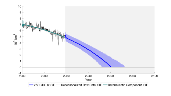
Figure 2: Trend Sea Ice Extent for September.
Shade is the 90% credible region.

For the two models, the median scenario has SIE being less than 1 $times$ $10^{6}$ km² by 2054 and 2060 respectively. The 1 $times$ $10^{6}$ km² is more likely an interesting quantity since the "regions north of Greenland/Canada will retain some sea ice in the future even though the Arctic can be considered as ’nearly sea ice free’ at the end of summer." (wang2009sea). The corresponding credible regions mark the period 2047-2065 for VARCTIC 8 and 2047-2069 for VARCTIC 18 respectively. These dates and time spans range in the close neighborhood of previous climate model simulations (see JahnEtAl2016). For both VARCTICs, less than 5% of the simulated paths hit 0 before 2050, making it an unlikely scenario according to our calculations. In essence, the two models suggest SIE melting at a rate that is slower than DieRu19’s results, but much faster than most CMIP5 models (StroeveEtAl12), and in line with the latest CMIP6 calculations (Notzetal2020).

Nonetheless, it is natural to ask how much we can trust a forecast made 40 years ahead, based on 40 years of data behind. To a large extent, answering this amounts to catalog what types of uncertainty the 90% credible regions incorporate, and those they do not. These reflect both forecasting uncertainty (the presence of shocks) and parameter uncertainty. The latter means the 90% regions reflect what happens to the spread of forecast paths when small disturbances are incorporated in the (estimated) coefficient matrix. In other words, those bands conveniently (and correctly) quantify prediction uncertainty accounting for the fact that we are iterating something that is estimated. All things considered, uncertainty is correctly calibrated as long as the model is correctly specified. As it is the case with any statistical approach, the VARCTIC necessarily assumes that the physical reactions estimated on previous decades’ data remain valid for those to come. Thus, if the future holds unprecedented nonlinear mechanisms or previously undetectable relationships, the VARCTIC can hardly accommodate for that. In contrast, any intensification of phenomena characterized by our 8 key variables (like Albedo feedback) should be successfully captured out-of-sample. With VARCTIC results being in accord with the recent CMIP6 consensus, our specification seems to capture the main drivers and dynamics of the Arctic ecosystem. Finally, future $CO_{2}$ emissions are an uncontested source of uncertainty for long-run SIE forecasts. Section 4.4 studies how those (and their credible regions) behave under standard forcing scenarios.

4.2 Impulse Response Functions

Figure 3 displays impulse response functions – the response of SIE to a positive shock of one standard deviation to any of the model’s M variables. To reflect parameter uncertainty, we additionally report the 90% credible region for each IRF. This means the gray bands contain 90% of the posterior draws from VARCTIC 8. Those are crucial to determine whether the attached IRFs describe significant physical phenomena or not. Particularly, when the credible region extends to both positive and negative sides, the IRF characterizes a phenomenon of negligible importance. In those instances (e.g., many IRFs at horizon $h>24$ months), the posterior mean’s (black line) difference from 0 could merely be due to parameter uncertainty, and can be thought of as approximately 0.

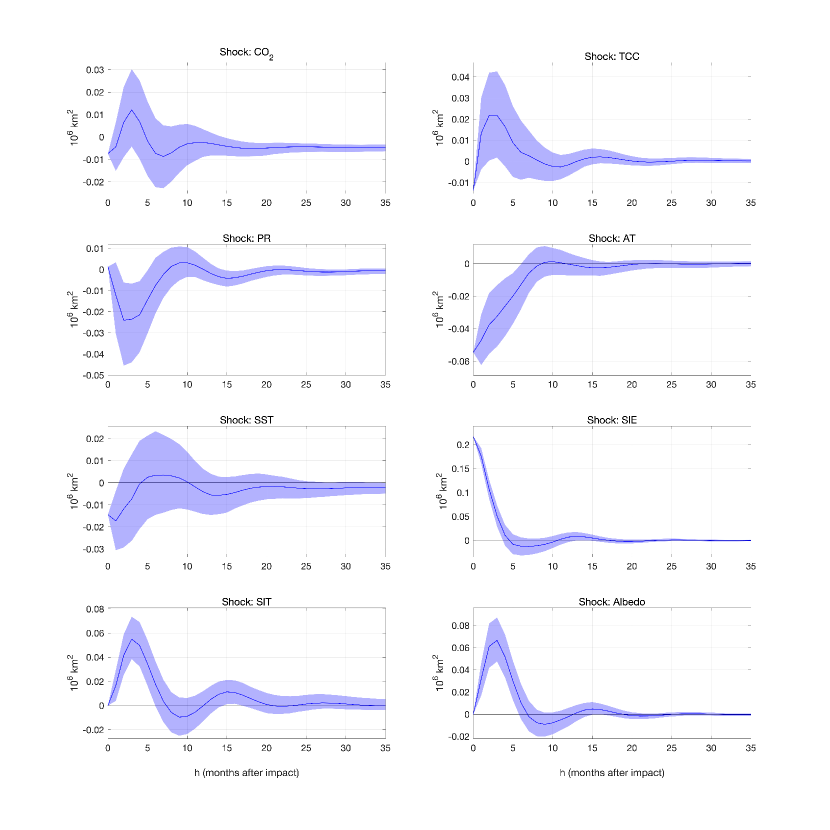
Figure 3: IRFs: Response of Sea Ice Extent.
Shade is the 90% credible region.

The resulting impact of $CO_{2}$ anomalies on SIE is sizable and most importantly, durable. While the sign of the response is highly uncertain and weak for more than a year, $CO_{2}$ shocks emerge to have a lasting downward effect on SIE. The relevance of the $CO_{2}$/SIE relation is not a surprise (notz2016observed). Moreover, this behavior is distinct from other shocks that rather have a significant short-run effect but no significant effect after more than roughly six months. More precisely, the effect of $CO_{2}$ impulses more than a year to settle in (not significant for approximately 15 months) but ends up having a continuing downward effect on trend SIE of approximately -0.005 $10^{6}$ km². This mechanically implies that a one-off $CO_{2}$ deviation from its predicted value/trend leads to a cumulative impact that is ever increasing in absolute terms (as displayed later in Figure 4(b)). It is important to remember that this is the effect of an unexpected increase in $CO_{2}$ which is to be contrasted with the systematic effect that will be studied later. However, in the framework of this section – where $CO_{2}$ is allowed to endogenously respond to Arctic variables – this is as close as one can get to obtain an experimental/exogenous variation needed to evaluate a dynamic causal effect. -0.005 $10^{6}$ is roughly 0.1% of the last deterministic trend value of SIE. $CO_{2}$ shocks, by construction of our linear VAR, have mean 0 and there are approximately as many positive and negative shocks in-sample. The linearity and symmetry of the VAR imply that these durable effects are present for both upward and downward deviations from the deterministic trend.

Figure 4: IRF Decomposition: Response of Sea Ice Extent.
Shade is the 90% credible region for the original IRF.

Other shocks have sizeable impacts that eventually vanish, which is the traditional IRF shape one would expect to see from a VAR on macroeconomic data. For instance, AT and Albedo IRFs clearly have the expected sign. However, they do not have the striking lasting impact of $CO_{2}$ perturbations. To rationalize the short-lived $IRF(\text{AT}\rightarrow\text{SIE})$, it is worth re-emphasizing what is meant by an AT shock. It is an AT anomaly that is not explicable by (i) the previous state of the system and (ii) other structural shocks ordered before it ($CO_{2}$, TTC, PR). As an example, one could think of the 2007 record low SIE (at that time) being attributed to an abnormally high “atmospheric flow of warm and humid air” from lower latitudes into the Arctic region (graversen2011). As we will see in section 4.3, a $CO_{2}$ shock triggers (with a significant delay) a persistent increase in AT, which eventually impacts SIE downward through the systematic part of the VAR. Thus, the short-lived response of SIE to AT shocks does not rule out a lasting impact of AT on SIE. Rather, it means that when it occurs, the origin of the anomaly is not AT itself, but likely $CO_{2}$.

Similar to an unforeseeable AT shock, a one-time Albedo shock will not have a lasting effect on SIE neither. This does not preclude Albedo to amplify other shocks as we will see in the next section. Finally, a rightful concern is whether IRFs remain unaltered upon sensibly altering the ordering of section 3.3. To a large extent, they do. For instance, placing SST and AT before TCC and PR brings no noticeable change. So does moving Albedo from last to second (see section A.4).

4.3 Amplification of $CO_{2}$ and Temperature Shocks by Feedback Loops

The melting of SIE is happening much faster than many other phenomena that are also believed to be set in motion by the steady increase of $CO_{2}$ emissions. Many recent papers (notz2012observations, wang2012sea, serreze2015arctic, notz2017arctic) argue with theory/climate models or correlations that external $CO_{2}$ forcing is responsible for the long-run trajectory of SIE. Some of these findings led notz2016observed to conclude that climate models severely underestimate the impact of $CO_{2}$ on SIE.

A rather consensual view is that the very nature of the Arctic system leads to the amplification of such external forcing shocks. An understanding – from observational data – on how the Arctic may amplify – or not – certain external forces is still pending. Fortunately, a VAR can quantify the contribution of different variables in explaining how a dynamic system responds to an external impulse.

4.3.1 Methodology

A potential approach that has a long history in econometrics is the use of Granger Causality (GC) tests. Those consist of evaluating predictive causal statements (such as $X_{t-1}\rightarrow Y_{t}$ and $Y_{t-1}\rightarrow X_{t}$) via significance tests in time series regressions. They have been recently advocated for climate applications by mcgrawbarnes2018. Nevertheless, those tests often fall short of answering questions of interest. First, the meaning of the test is not obvious when more than two variables are included and/or if one is interested in multi-horizon impacts. Second, in the wake of a GC test rejection, the block of reduced-form coefficients, which we know to be of some statistical importance, are very hard to interpret. In other words, we know some channel matters, but we have little idea how it matters.

In light of the above, we rather opt for IRF Decomposition. As the name suggests, the physical reaction characterized by IRFs will be decomposed as a sum of transmission channels, which contributions’ magnitudes and signs are directly informative. Less abstractly, the consequential negative response of SIE to $CO_{2}$ shocks is likely composed of a direct effect and many entangled indirect effects (e.g., that of AT and Albedo). Understanding those in the dynamic setup of a VAR is much more intricate than in a static regression setting. This is so because IRFs – for horizons greater than one – are obtained by iterating predictions, which means $X$ can impact $Y$ through $Z$, but also through any of its lags. We employ a strategy that has been used in macroeconomics to better understand the transmission mechanism in VARs. It consists, rather simply, of shutting down "channels" and plotting what the response to a shock would be, given that this very channel had been shut (sims2006does, bernanke1997systematic, bachmann2012confidence). We can deploy this methodology to find and quantify the most important channels through which $CO_{2}$ and temperature shocks impact SIE.

4.3.2 Amplification of $CO_{2}$ Shocks

For VARCTIC 8, figures 4(a) and 4(b) show the responses of SIE to an unexpected increase in one standard-deviation of $CO_{2}$. The blue line pictures the case of the baseline VARCTIC 8 with 90% credible region. The remaining six lines show the response of SIE to the same shock but shutting down key transmission channels. In terms of implementation, it consists of imposing hypothetical shocks to one of the other variables which off-sets their own response to a $CO_{2}$ shock.

The top panel of figure 4 reveals – without great surprise – the importance of temperature (especially AT) in translating $CO_{2}$ anomalies into decreasing SIE. That is, we observe that shutting down these channels leads to a smaller absolute response which means that those variables can be considered as amplification channels. Given the atypical shape of the $CO_{2}$ IRF, the scale of figure 4(a) makes less visible the action of channels that only alter the longer-run effect. Since those effects are durably negative (at different levels), their cumulative effect will more clearly reveal their relative importance. Thus, figure 4(b) displays the cumulative impact of selected (more important) channels. The two temperature channels are responsible for approximately one fourth of the cumulative effect of $CO_{2}$ on SIE after 3 years. More precisely, restricting temperature variables to not respond to a positive $CO_{2}$ shock, decreases (in absolute terms) the after-3-years impact from -0.13 $10^{6}$ km² to -0.1 $10^{6}$ km². Of course, it was expected that temperature should be a major conductor of such shocks. We also observe similar quantitative effects for both SIT and Albedo in isolation. Most strikingly, we find that the conjunction of the Albedo and SIT amplification channels is responsible for amplifying the effect of $CO_{2}$ shocks by a non-negligible 50%.

The Albedo-amplification matches evidence reported in several studies (see Pero2012, Bjoerk2013, Park13) using various different methodologies. In contrast, our results for SIT-amplification contribute to a literature where a consensus has yet to emerge. The ice-growth-SIT feedback describes the observation that a thinning of the sea ice cover induces more rapid ice formation during winter, a compensating effect which slows down melting (bitz2004mechanism; GoosseEtAl2018). Other studies have emphasized the positive feedback between $SIT$ and $SIE$, where a thinning ice cover further accelerates melting by being less resilient to climate forcing (Park13; Kwok2018). Our results unequivocally support the latter to be most empirically prevalent. Nearly identical results are obtained when using AT, Albedo, PR, and TCC averaged between 60^∘N and 90^∘N latitude, suggesting most (if not all) of the action comes from higher latitudes – hence our focus on local processes when explaining those results.

This section focused on how and why SIE responds to $CO_{2}$ shocks. In section 4.4, we rather look at the effect of the systematic increase of $CO_{2}$ level.

4.3.3 Amplification of Air Temperature Shocks

AT-shocks are movements in AT that are not predictable given the past state of the system and are orthogonal to other shocks in the system, most notably $CO_{2}$. In other words, we are looking at the effect of unexpected higher/lower AT that is uncorrelated with other shocks in the system. As we saw in figure 3, such AT anomalies have a pronounced short-run effect on trend SIE for no longer than ten months after the shocks. This means that unlike $CO_{2}$, the cumulative effect of AT disturbances stabilizes about 1.5 years after the event.

In figure 4(c), we clearly observe (again) an important role for the thinning of ice and the Albedo effect amplifying the response of SIE to AT shocks. In fact, we see in figure 4(d) that without them, the long-run impact is the same as the instantaneous one. Thus, this is evidence to suggest that the AT shock’s long-run cumulative impact of -0.24 $10^{6}$ km² is mostly a result of the action of feedback loops.

4.4 Forecasting SIE Conditional on $CO_{2}$ Emissions Scenarios

If $CO_{2}$’s trend is mostly or solely affected by factors outside of those considered in the VAR, the forecast of SIE can be improved by treating $CO_{2}$ forcing as exogenous and using an external forecast rather than the one internally generated by the VAR. Conditional forecasting can be achieved in VARs following the approach of waggoner1999conditional. As we will see, this will markedly sharpen the bands around our forecasts, suggesting that a great amount of uncertainty is related to the future path of $CO_{2}$ emissions. Additionally, this brings the VARCTIC conceptually closer to standard analyses on the future of the Arctic (StroeveEtAl12, stroeve2018, Notzetal2020).

In the spirit of SigmondEtAl2018, who constrain the levels of AT in their climate model, we will look at $CO_{2}$ emissions under three different representative concentration pathways (RCP) and investigate their impact on the evolution of Arctic sea ice. Figure 1 shows a steady increase in $CO_{2}$ emissions over the last three decades, but several RCPs paint different pictures for the trajectory of carbon emissions until the end of the century. Figure 5(a) shows the different paths of $CO_{2}$ under RCP 2.6, RCP 6, and RCP 8.5, as well as the projected path following VARCTIC 8. Most interestingly, we find our completely endogenous and unconditional forecast of $CO_{2}$ to lay somewhere between the "very bad" RCP 8.5 scenario and the "business-as-usual" RCP 6 one.

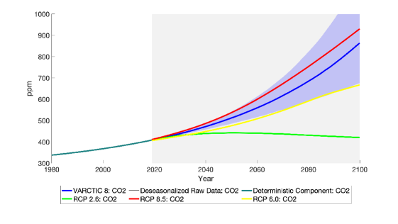
(a) Evolution of CO₂ emissions until the End of the Century under different Scenarios

(b) Evolution of SIE under different Scenarios of $CO_{2}$

Figure 5: VARCTIC Projections & Different RCPs.
Shade is 90% credible region.

Figure 5(b) shows VARCTIC 8’s projection of Arctic SIE when conditioning the out-of-sample path of $CO_{2}$ on the three different RCP scenarios. For reference, the figure also includes projected SIE with the future path of $CO_{2}$ endogenously determined within the model, as discussed above. The pictured effect is dramatic: if emissions were reduced as to follow the RCP 2.6 scenario, whose $CO_{2}$ emissions are still at the higher boundary of what the Paris Agreement demands, the Arctic would be far from blue and even recover earlier losses by the end of the century. If emissions follow the more likely RCP 6, SIE would vanish later than projected by the unconditional VARCTIC 8, but would still be completely gone during the 2070’s. In the worst-case scenario, RCP 8.5, we obtain an ice-free September by the mid-2050’s. Interestingly, this result is very close to what stroeve2018 reported using a very different methodology (extrapolating a linear relationship). Their bivariate (SIE and $CO_{2}$) analysis suggests the Arctic summer months to be ice-free by 2050. However, in contrast, our results are much more optimistic than theirs in terms of SIE conditional on the (rather unlikely) RCP 2.6 scenario. Such analysis is not conditional on the identification scheme since it is based solely on the reduced form. Overall, these results reinforce the view that anthropogenic $CO_{2}$ is the main driver behind the current melting of SIE as well as the main source of uncertainty around the future SIE path. Furthermore, the optimistic RCP 2.6 results suggest that internal variability by itself cannot lead to the complete melting of SIE, even when starting from today’s level. Overall, the VARCTIC yields similar conclusions about the importance of $CO_{2}$ to that of DaiLuoSong19 and notz2016observed. It is reassuring to see that climate models’ conclusions can be corroborated by a transparent approach that relies solely and directly on the multivariate time series properties of the observational record.

4.5 Amplification Effects in the Projection of SIE under different RCPs

The previous section documented the evolution of SIE conditional on several $CO_{2}$ trajectories, treating the latter as an exogenous driver. This section seeks to quantify the importance of feedback effects when it comes to translating an RCP path into SIE loss. That is, we attempt to quantify to which extent the Albedo- and SIT-effects can be held responsible for amplifying the impact of $CO_{2}$ forcing and thus accelerating the melting of SIE.

Following the findings of section 4.3, in which we identified SIT and Albedo to carry potential for mitigating the adverse influence of $CO_{2}$ on SIE, we ask the question about how SIE would evolve, if SIT and Albedo were to remain constant at a certain level over the forecasting period. In particular, we repeat the forecasting exercise of the previous section for all three RCP scenarios, but keep SIT and Albedo constant until the end of the forecasting period. For both variables we set the level equal to the value, which is given by the series’ deterministic component at the end of the sample period. By doing so, we create artificial shocks to both SIT and Albedo in each forecasting step, which off-set their response to the external forcing variable. As we are modeling a dynamic and interconnected system, these shocks do affect all the other variables (except for $CO_{2}$ on which we condition our forecast).

Figure 6 documents the corresponding results for RCP 8.5, RCP 6 and RCP 2.6. For each scenario, we show three different cases: (i) the projection of SIE under the respective RCP; (ii) the evolution of SIE under the respective RCP while keeping Albedo constant at its last in-sample deterministic value; (iii) the projection of SIE while keeping both Albedo and SIT constant at their last respective deterministic value. The latter are shown to be undeniable accelerants. First, fixing Albedo to its 2019 value and thus shutting down this particular long-run amplification effect postpones the date of reaching $1\times 10^{6}$ $km^{2}$ by a bit less than a decade under both RCP 8.5 and RCP 6. Arctic sea ice thickness plays a major role for the reaction and resilience of SIE to anthropogenic forcing. Figure 6 re-enforces this view by showing that preventing both SIT and Albedo from further decay could potentially postpone the zero-SIE event to the next century under RCP 6. Under RCP 8.5, shutting down both amplification channels starting from 2020 leads to SIE crossing the bar of $1\times 10^{6}$ $km^{2}$ about a decade later. This feeds into the pictured non-linearity and acceleration of SIE loss and provides a potential justification for the finding in DieRu19 that a quadratic trend is a preferable approximation of long-run summer months’ SIE evolution.

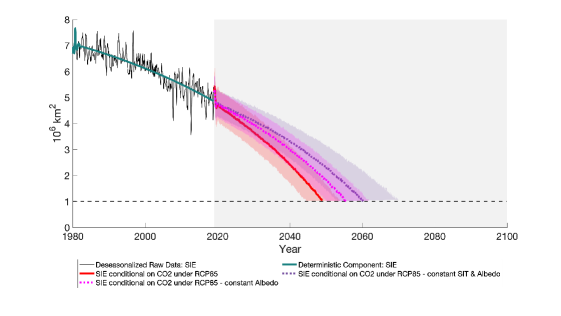
(a) RCP 8.5

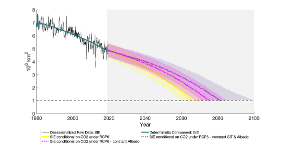
(b) RCP 6

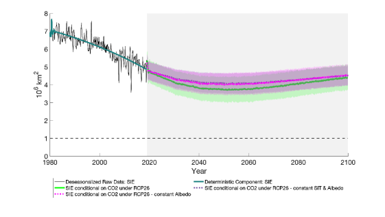
(c) RCP 2.6

Figure 6: Conditional Forecasts with and without Feedback

5 Conclusion and Directions for Future Research

We proposed the VARCTIC as a middle ground alternative to purely theoretical or statistical modeling. It generates long-run forecasts that embody the interaction of many key variables without the inevitable opacity of climate models. First, we focus our attention on how the Arctic system responds to exogenous impulses and propagates them. Our results show that $CO_{2}$ anomalies have an unusually lasting effect on SIE which takes about a year to settle in. It is the only impulse that has the property of durably affecting SIE. Albedo and SIT are shown to play an important role in amplifying the response of SIE to $CO_{2}$ and AT shocks. In both cases, the conjunction of the two effects can double the cumulative impact of such shocks after two years.

Second, we focus on the systematic/deterministic part of the VARCTIC and conduct conditional forecasting experiments that again seek to quantify the effect of anthropogenic $CO_{2}$ and how feedback loops can amplify it. We condition on the future path of $CO_{2}$ and show that, within the context of our model, it is the prime source of uncertainty for the long-run forecast of SIE. RCP 8.5 implies 0 September SIE around 2054, RCP 6 says so around 2075 and finally, RCP 2.6 ($\sim$ Paris Accord) implies that such an event would never happen. We conclude the analysis by evaluating to which extent internal knock-on effects can amplify the long-run effect of $CO_{2}$ forcing. Our results provide statistical backing for the view that $CO_{2}$ shocks trigger feedbacks of other climate variables (as characterized here by Albedo and SIT), which substantially accelerate the speed at which SIE is headed toward 0.

There are many methodological extensions within the VAR paradigm that could be of interest for future cryosphere research. For instance, Smooth-Transition VARs (with a popular application in AG2012) could be used to accommodate for dynamics evolving over the seasonal cycle. Additionally, ScreenDeser2019 remark the importance of changing weather phenomena that transition through decadal cycles, such as the pacific oscillation. Time-varying parameters VARs could evaluate the quantitative relevance of such phenomena. Finally, some recent attention (chavas2019dynamic) has been given to the potentially non-linear relationship between $CO_{2}$ and SIE. Methods that blend time series econometrics and Machine Learning of the like in GC_MRF could reveal interesting insights on complex/time-varying relationships in the Arctic.

Appendix A Appendix

A.1 Data Sources

Table 1: List of Variables

Abbreviation	Description	Data Source
Age	Gridded monthly mean of Sea Ice Age	EASE-Grid Sea Ice Age, Version 4
AT	Gridded monthly mean of Air Temperature	NCEP/NCAR Reanalysis 1: Surface
Albedo	Gridded monthly mean of Surface Albedo	MERRA-2
$CO_{2}$	Global monthly mean of $CO_{2}$	NOAA - Earth System Research Laboratories
LWGAB	Gridded monthly mean of Surface Absorbed Longwave Radiation	MERRA-2
LWGEM	Gridded monthly mean of Longwave Flux Emitted from Surface	MERRA-2
LWGNT	Gridded monthly mean of Surface Net Downward Longwave Flux	MERRA-2
LWTUP	Gridded monthly mean of Upwelling Longwave Flux at TOA	MERRA-2
PR	Gridded monthly mean of Precipitation	CPC Merged Analysis of Precipitation (CMAP)
SST	Median northern-hemispheric mean Sea-Surface Temperature anomaly (relative to 1961-1990)	Met Office Hadley Centre
SIE	Gridded monthly mean of Sea Ice Extent	Sea Ice Index, Version 3
SWGNT	Gridded monthly mean of Surface Net Downward Shortwave Flux	MERRA-2
SWTNT	Gridded monthly mean of TOA Net Downward Shortwave Flux	MERRA-2
TAUTOT	Gridded monthly mean of In-Cloud Optical SIT of All Clouds	MERRA-2
SIT	Gridded monthly mean of Sea Ice Thickness	PIOMAS
TCC	Gridded monthly mean of Total Cloud Cover	NCEP/NCAR Reanalysis Monthly Means and Other Derived Variables
TS	Gridded monthly mean of Surface Skin Temperature	MERRA-2

• Notes: The above series (before any transformation) are gathered in one file here.

A.2 Transmission Mechanism Analysis for a Shock to SIE

The purpose of the TMA analysis is to assess how the response of variable $i$ to a shock on variable $j$ changes, if a third variable $z$ were immune to the shock generated by variable $j$. Here we follow Sims12 by differentiating between the direct and indirect effect. The former is variable $i$’s own response to the shock hitting variable $j$. However, the shock also affects variable $z$, which itself transmits the shock further to variable $i$. This channel is the indirect effect of a shock to variable $j$ on the response of variable $i$. Hence, it is the latter that will explain the role of variable $z$ within the transmission channel of a shock to $j$ on $i$. To do so, Sims12 introduce artificial shocks to variable $z$, which offset its own response to a shock to $j$. These artificial shocks have two effects: (i) the IRF of variable $z$ will be zeroed over the whole IRF horizon; (ii) the indirect channel transmits the artificial shock onto variable $i$ and allows to identify the direct effect of $j$ on $i$.

This procedure requires the transformation of the structural VAR, given in equation (2) into the reduced form VAR of equation (3), which reads as follows:

$$\bm{y}_{t}=\bm{c}+\sum_{p=1}^{P}{A^{-1}\Psi_{p}}\bm{y}_{t-p}+A^{-1}\bm{\varepsilon}_{t}\qquad,$$ (A.1)

where $A^{-1}$ is the Cholesky decomposition of matrix $A$ in equation (2). This imposes the necessary restrictions in order to identify the contemporaneous relationships of the variables. In particular, it assumes higher ordered variables to have an immediate effect on variables that are ranked below, but not vice versa. As $CO_{2}$ is ordered first in all of our models, an exogenous shock to carbon dioxide in period $t$ will have an immediate effect on all of the other variables. The companion form of equation (A.1) is

$$\bm{Y}_{t}=\bm{c}+\Phi\bm{Y}_{t-1}+A^{-1}\bm{\varepsilon}_{t}\enskip,$$ (A.2)

where $\bm{Y}_{t}=\left[y_{t}\;y_{t-1}\;\cdots\;y_{t-p-1}\right]^{\top}$ and the corresponding companion matrix is

$$\Phi=\begin{pmatrix}A^{-1}\Psi_{1}&A^{-1}\Psi_{2}&\cdots&\cdots&A^{-1}\Psi_{p}\\ I&0&0&\cdots&0\\ 0&I&0&\cdots&0\\ \vdots&\vdots&\ddots&\vdots&\vdots\\ 0&\cdots&\cdots&I&0\end{pmatrix}\enskip.$$ (A.3)

An equivalent way (to what laid out in section 3.4) of constructing IRFs, i.e. the response of variable $i$ to a structural shock on variable $j$ over all horizons $h=0,...,H$, is to proceed iteratively. Hence, for a given period $h$, the response of $i$ to a shock hitting $j$ is given by

$$IRF(j\rightarrow i,h)=e_{i}\Phi^{h}A_{\bullet,j}^{-1}$$ (A.4)

where $e_{i}$ is a selection vector of dimension $1\times M$ with 1 at entry $i$ and 0 otherwise. $A_{\bullet,j}^{-1}$ elicits the $j^{th}$ column of $A^{-1}$. Following Sims12, switching off the indirect effect of a shock to variable $j$ on $i$ via variable $z$ amounts to $IRF(j\rightarrow z,h)=0\;\forall\;h=0,...,H$. That requires the artificial shocks, $\varepsilon_{z,h}$, to be calibrated such that the response of variable $z$ to a shock to variable $j$ is zero over the whole IRF period. Hence, at $h=1$ the artificial shock $\varepsilon_{z,1}$ is

$$\varepsilon_{z,1}=-\frac{A^{-1}_{j,1}}{A^{-1}_{z,1}}\enskip.$$ (A.5)

As these shocks are transmitted through time, the artificial response $\varepsilon_{z,h}$ has to account for all the past shocks, $\varepsilon_{z,h-1}$, for any periods beyond $h=1$:

$$\varepsilon_{z,h}=-\frac{IRF(j\rightarrow z,h)+\sum^{h-1}_{h^{\prime}=0}e_{z}\Phi^{h-h^{\prime}}A^{-1}_{\bullet,j}\varepsilon_{z,h^{\prime}}}{e_{z}A^{-1}_{z}}\enskip.$$ (A.6)

The altered IRFs (that omits the transmission channel $z$) for all the variables in the model to a shock to $j$ is

$$IRF_{-z}(j\rightarrow\bm{i},h)=IRF(j\rightarrow\bm{i},h)+\sum^{h}_{h^{\prime}=0}e_{z}\Phi^{h-h^{\prime}}A^{-1}_{\bullet,j}\varepsilon_{z,h^{\prime}}\enskip.$$ (A.7)

So far, we have reviewed how IRF decomposition works when one is interested in shutting down a single channel at a time. In contrast to Sims12, our VAR comprises more than three variables. Therefore, in some cases, it is desirable to shut-down not only one, but a group $Z\in M\setminus\left\{i,j\right\}$ of indirect channels. To do so, equations (A.5) and (A.6) need to be generalized. At impact, the artificial response of variable $z$ to a shock to $j$ does not only have to offset the direct effect of $j$, but also the indirect effect of a shock $j$ via the indirect effect of all the other artificial responses ($\bm{\varepsilon^{+}_{z^{+},1}}$) of those variables in $Z$ which are ordered above $z$. This amounts to the following extension of equation (A.5):

$$\varepsilon_{z,1}=-\left(\frac{A^{-1}_{j,1}}{A^{-1}_{z,1}}+\frac{\sum_{m\in z^{+}}\varepsilon_{m,1}}{A^{-1}_{z,1}}\right)\enskip.$$ (A.8)

Also equation (A.6) has to be adjusted accordingly. However, at horizons $h>1$ the artificial response $\varepsilon_{z,h}$ will not only have to offset the contemporaneous effects of $z^{+}$, but also compensate for the artificial responses of all other variables in $Z$ over the period $h^{\prime}=0\;\cdots\;h-1$:

$$\varepsilon_{z,h}=-\frac{IRF(j\rightarrow z,h)+\sum^{h-1}_{h^{\prime}=1}e_{z}\Phi^{h-h^{\prime}}A^{-1}_{j}\varepsilon_{z,h^{\prime}}+\sum^{h-1}_{h^{\prime}=1}\sum_{n\in Z}\varepsilon_{n,h^{\prime}}+\sum_{m\in z^{+}}\varepsilon_{m,1}}{e_{z}A^{-1}_{z}}\enskip.$$ (A.9)

Equation (A.7) for the modified IRF ($IRF_{-z}(j\rightarrow\bm{i},h)$) remains intact.

A.3 Bayesian Estimation Details

Bayesian inference implies the use of priors, which degree of informativeness is usually determined by the user. To be as agnostic as possible, we use the technique of giannone2015prior to choose the tightness of priors as to optimally balance bias and variance in a data-driven way. The prior structure, however, must be chosen. We estimate our benchmark Bayesian VARCTIC with a standard Minnesota prior. In this simple framework, $\bm{\Sigma}$, the variance-covariance matrix of the VAR residuals, is treated as known. Thus, the remaining parameters of the model reduce to the vectorized matrix $\beta=vec\left(\left[\bm{\Phi_{1}}\cdots\bm{\Phi_{p}}\;\textbf{c}\right]^{\top}\right)$ of dimension $(M^{2}p+M)\times 1$. The posterior distribution of $\beta$, $\pi\left(\beta|y\right)$, is obtained by the product of the likelihood function of the data $f\left(y|\beta\right)$, and the prior distribution of $\beta$, $\pi\left(\beta\right)$. Hence, by sampling from the posterior distribution $\pi\left(\beta|y\right)\propto f\left(y|\beta\right)\pi\left(\beta\right)$ we can quantify both the uncertainty around $\beta$, but also more interesting transformations of it, such as IRFs and forecasts. The prior distribution for $\beta$ is the multivariate normal distribution $\pi\left(\beta\right)\sim N\left(\beta_{0},\Sigma_{0}\right)$. The Minnesota prior is a specific structure for values of both $\beta_{0}$ and $\Sigma_{0}$. In words, it allows concisely to parameterize heterogeneity in both the prior mean and variance. It consists of three major elements: the first one is about $\beta_{0}$ and the last two concern $\Sigma_{0}$.

1. For any equation $y_{m,t}$ with $m=1,...M$ – where $M$ is the total number of observed variables in the VAR – all parameters are shrunk to 0 except for its first own lag $y_{m,t-1}$. The latter is usually shrunk to a value $b_{AR}$ between 0.5 and 1. This can be interpreted as shrinking each VAR equation to the much simpler and parsimonious AR(1) process. Given the persistent nature of time-series data, this structure for $\beta_{0}$ is much more appropriate than that of Ridge regression (or LASSO), which shrinks all coefficients homogeneously towards 0.

2. It is often observed in multivariate time series models that $y_{m,t-1}\rightarrow y_{m,t}$ will be way stronger than almost any of the $y_{\tilde{m},t-1}\rightarrow y_{m,t}$ (with $\tilde{m}\neq m$) relationships. $\lambda_{2}$ therefore calibrates the relative intensity of shrinking dynamic cross-correlations versus that of autocorrelations.

3. Distant partial lag relationships (say $y_{m,t-12}\rightarrow y_{m,t}$) are expected to be of smaller magnitude than close ones like $y_{m,t-1}\rightarrow y_{m,t}$, and $y_{m,t-2}\rightarrow y_{m,t}$. $\lambda_{3}$ determines the additional intensity of distant lags shrinkage.

The overall tightness of the prior apparatus is determined by $\lambda_{1}$. To draw a parallel to penalized regression (like Ridge and LASSO), a small $\lambda_{1}$ in a Bayesian VAR increases regularization in a way analogous to increasing the $\lambda_{RIDGE}$ – that is, by pushing the BVAR estimate $\hat{\Phi}$ away from $\hat{\Phi}_{OLS}$. Following giannone2015prior, we optimize/estimate hyperparameters within some grid and the total number of posterior draws is 2000. The optimal values for VARCTIC 8 are $\{b_{AR},\lambda_{1},\lambda_{2},\lambda_{3}\}=\{0.9,0.3,0.5,1.5\}$. We fix the number of lags in VARCTIC 8 to $P=12$ and to $P=3$ in VARCTIC 18 respectively.

Finally, given the very smooth look of deseasonalized $CO_{2}$ in Figure 1, one could worry that it merely acts as a proxy for an omitted linear trend. We view the use of trends as undesirable in our multivariate setup as it would undermine the capacity of the VARCTIC to be a "complete" model. Including a trend would make it rely on an unknown/unexplained latent force – which is at odds with the main goal of our modeling strategy. For the sake of completeness, we nevertheless estimate such models to find out that the inclusion of an exogenous time trend is in fact not preferred by the data according to the Deviance Information Criterion (DIC, a generalization of the well-known AIC). VARCTIC 8 has a DIC of -6894.35 and adding an exogenous trend makes it -6817.32. The smallest value being preferred, this justifies on a data-driven basis the exclusion of the trend. While seemingly technical of point, this means the VARCTIC 8 system, based solely on dynamic relationships of observable data, can generate/simulate the observed SIE downward path.

A.4 Different Ordering

In this section, we check the sensitivity of the responses of SIE to a shock of any of the other variables when varying the ordering of variables compared to the benchmark VARCTIC 8 in section 4. The priors and lags remain unaltered to the specification outlined in section A.3. The ordering now reads: $CO_{2}$, AT, SST, TCC, PR, SIE, SIT, Albedo.

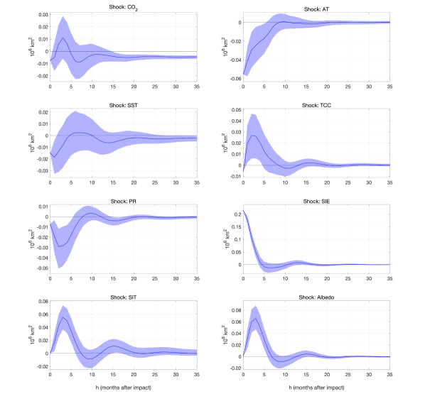
Figure 7: IRFs: Response of Sea Ice Extent

A comparison of the responses of the benchmark VARCTIC 8 in Figure 3 and the IRFs after reordering the model (Figure 7) documents the robustness of results to different identification schemes. A second – more radical – variation in the model set-up locates Albedo at position two. Hence, a shock to Albedo will contemporaneously affect all the other variables except $CO_{2}$: $CO_{2}$, Albedo, TCC, PR, AT, SST, SIE, SIT.

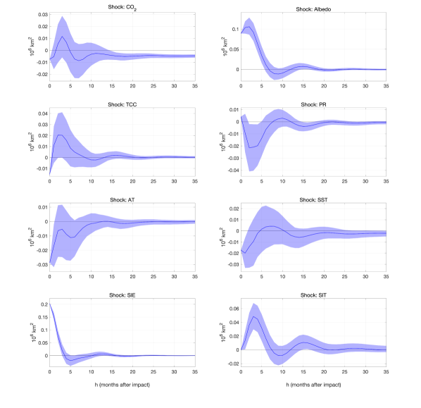
Figure 8: IRFs: Response of Sea Ice Extent

For most of the effects, the shapes remain robust in comparison with Figure 3. Only the response to air temperatures deviates visibly with the statistically significant impact in the short-run now vanishing.

A.5 Results of VARCTIC 18

VARCTIC 18, including all the variables in Table 1, tests the robustness of VARCTIC 8 projection of SIE. The ordering of variables in VARCTIC 18 reads as follows: SWGNT, SWTNT, $CO_{2}$, LWGNT, TCC, TAUTOT, PR, TS, AT, SST, LWGAB, LWTUP, LWGEM, SIE, Age, SIT, EMIS and Albedo. Due to the increased number of variables, the lags were reduced to 3 and the estimation period starts in 1984 due to some series unavailability. With more parameters to estimate, the prior specification slightly tightens to $\{b_{AR},\lambda_{1},\lambda_{2},\lambda_{3}\}=\{0.8,0.5,0.5,3\}$.

The forecasts of SIE under the specification of VARCTIC 18 are all reported in Figure 9. This includes both the unconditional forecast and those conditional on RCP’s. The median unconditional VARCTIC 18 forecast a blue Arctic in September 2062, which is in the very neighborhood of VARCTIC 8. This result suggests VARCTIC 8 to comprise the key variables for a proper and robust long-run projection of Arctic sea ice. The projected ice-free dates under the RCP 6 and RCP 8.5 scenarios are also consistent with the results reported by VARCTIC 8 in Figure 5(a). The trajectory of SIE under RCP 2.6, however, slightly changes and seems to stabilize rather than recover by the end of the century.

The IRFs of SIE are shown in Figure 10. Those of key variables (as included in VARCTIC 18) remain roughly unchanged in VARCTIC 18. Most interestingly, in VARCTIC 18, not only $CO_{2}$ shock has the effect of triggering a durably decreasing SIE, but also LWGAB, which measures the longwave radiation absorbed by the surface and AT. Many other shocks have significant impacts in the short run but only $CO_{2}$, LWGAB, and AT shocks have the unique property of durably pushing the system out of the former equilibrium.

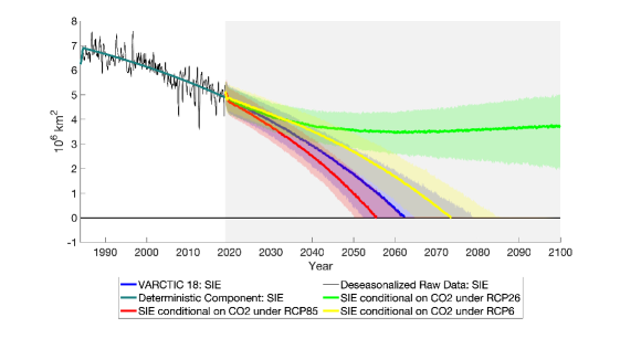
Figure 9: Evolution of SIE different scenarios of $CO_{2}$ in VARCTIC 18

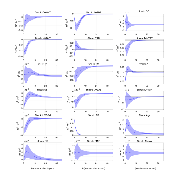
Figure 10: IRFs: Response of Sea Ice Extent in VARCTIC 18. Shade is the 90% credible region.

A.6 Stochastic De-seasonalization

As a robustness check, we verify that our main results hold if we employ a radically different technique to take out seasonality. In this subsection, we adopt the approach of structural time series (Harvey90 and harvey2014) where $y^{raw}$ is split into three somewhat intuitive parts:

$$y_{t}^{raw}=\mu_{t}+\gamma_{t}+\eta_{t}$$

a trend component $\mu_{t}$; a seasonality component $\gamma_{t}$ and a (possibly autocorrelated) noise component $\eta_{t}$. Each of them is stochastic and has its own law of motion. The structure and law of motions we use follow the well-established Harvey Basic Structural Model (harvey1983). The model reads as follows:

$$\mu_{t}=\mu_{t-1}+\beta_{t}+u_{t}$$

$$\beta_{t}=\beta_{t-1}+v_{t}$$

$$\gamma_{t}=-\sum_{m=1}^{11}\gamma_{t-m}+w_{t}$$

$$\left(\eta_{t},u_{t},v_{t},w_{t}\right)\leavevmode\nobreak\ \sim\leavevmode\nobreak\ iid\,N\left(0,\leavevmode\nobreak\ \Sigma\right)$$

$$\Sigma=\begin{pmatrix}\sigma^{2}_{\eta\eta}&0&0&0\\ 0&\sigma^{2}_{uu}&0&0\\ 0&0&\sigma^{2}_{vv}&0\\ 0&0&0&\sigma^{2}_{ww}\\ \end{pmatrix}$$

The law of motion is that of harvey1983 and fits in a traditional state space model. The trend $\mu_{t}$ is a random walk with a stochastic drift. The drift $\beta_{t}$ is itself evolving according to a random walk. For instance, this means that $\mu_{SIE,t}$, the trend of SIE, is trending down stochastically at a rate $\beta_{SIE,t}$. That (negative) growth rate is itself allowed to evolve. A quick look at a flexibly modeled trend of SIE suggests that allowing for a time-varying growth rate is necessary given the acceleration and deceleration of SIE melting in the 2000’s. Figure 11 shows the complete set of stochastic trends resulting from the BSM.

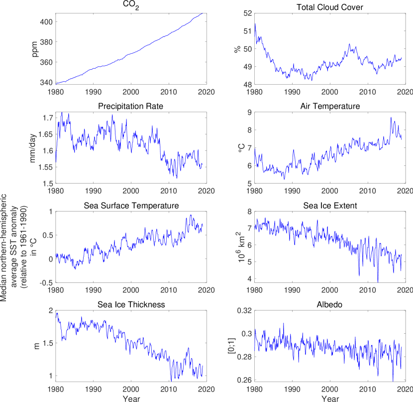
Figure 11: Basic Structural Model: 8 Variables
Extracted Trends adjusted for average September-Seasonality

The extraction of trends as a first step and their subsequent modeling as a second step is analogous to standard practice in macroeconomics, but not similar. In macroeconomics, it is customary in a strand of empirical work to filter the data as a pre-processing step. The VAR is then estimated on the extracted cycles, which is simply the difference of the raw data and the estimated trend. Here, we are indeed doing the filtering step first but using trend components – rather than seasonality and short-run noise – for the second step. However, our trend components $\mu_{t}$ are rather stochastic with respect to what is usually seen in economics.

A.6.1 The Benchmark Specification and Results

Following giannone2015prior, we obtain the optimal hyperparameters:

• Autoregressive Coefficient: = 1;

• Overall tightness is $\lambda_{1}$ = 0.3;

• Cross-variable weighting is $\lambda_{2}$ = 0.5;

• Lag decay is $\lambda_{3}$ = 1.51;

• Exogenous variable tightness: $\lambda_{4}$ = 100;

The date of the zero-lower bound of the stochastic de-seasonalized version remains in the neighborhood of the benchmark model. In this specification, the Arctic would be ice-free by the year 2061.

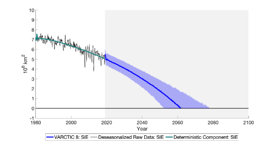
Figure 12: Trend Sea Ice Extent
Stochastic De-seasonalization

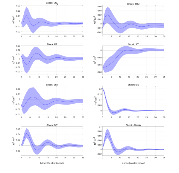
Figure 13: IRFs: Response of Sea Ice Extent
Stochastic De-seasonalization

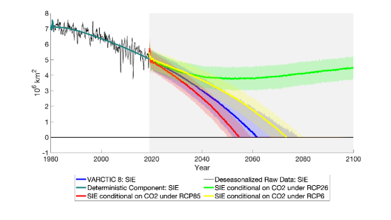
Figure 14: Evolution of SIE under different Scenarios of $CO_{2}$
Different Scenarios
Stochastic De-seasonalization - Extracted trend adjusted for mean September-seasonality

As the BSM specification allows for evolving seasonality, we can also use it to obtain more flexible month-specific VARCTICs. The benchmark specification implies that we can transform our series into a string of "synthetic" Septembers or Marchs by simply adding or subtracting a constant. In the evolving seasonality model, one can rewrite a slowly widening seasonal pattern as the expression of heterogeneous trends across seasons. Thus, rather than adding back the mean (over time) of $\gamma_{t,September}$ to $\mu_{t}$ to fit the model on static synthetic Septembers, we can add back

$$\tilde{\gamma}_{t,September}=\sum_{t^{\prime}=1}^{T}I(t^{\prime}=t){\gamma}_{t^{\prime},September}$$

to model evolving synthetic Septembers (or any month of interest). Unlike our benchmark specification, this approach allows for summer vs non-summer months to have different trends. Figure 15 reports results of our conditional forecasting analysis conducted for two radically different months. While March’s SIE is linearly trending in-sample, the projections suggest a potential acceleration of melting in the second half of the century – with widening uncertainty.

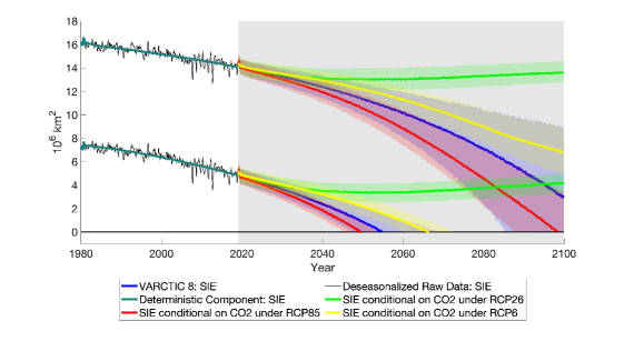
Figure 15: Evolution of SIE under different Scenarios of $CO_{2}$
Different Scenarios
Stochastic De-seasonalization:
Extracted trend adjusted for yearly September- & March-seasonality

References

- Amstrup et al. (2010) Amstrup, S., E. DeWeaver, D. Douglas, B. Marcot, G. Durner, C. Bitz, and D. Bailey, 2010: Greenhouse gas mitigation can reduce sea-ice loss and increase polar bear persistence. Nature, 468 (37326), 955–958, URL https://doi.org/10.1038/nature09653.
- Auerbach and Gorodnichenko (2012) Auerbach, A. J., and Y. Gorodnichenko, 2012: Measuring the output responses to fiscal policy. American Economic Journal: Economic Policy, 4 (2), 1–27.
- Bachmann and Sims (2012) Bachmann, R., and E. R. Sims, 2012: Confidence and the transmission of government spending shocks. Journal of Monetary Economics, 59 (3), 235–249.
- Bańbura et al. (2010) Bańbura, M., D. Giannone, and L. Reichlin, 2010: Large bayesian vector auto regressions. Journal of applied Econometrics, 25 (1), 71–92.
- Bernanke et al. (2005) Bernanke, B. S., J. Boivin, and P. Eliasz, 2005: Measuring the effects of monetary policy: a factor-augmented vector autoregressive (favar) approach. The Quarterly journal of economics, 120 (1), 387–422.
- Bernanke et al. (1997) Bernanke, B. S., M. Gertler, M. Watson, C. A. Sims, and B. M. Friedman, 1997: Systematic monetary policy and the effects of oil price shocks. Brookings papers on economic activity, 1997 (1), 91–157.
- Bhatt et al. (2019) Bhatt, U., and Coauthors, 2019: Sea ice outlook: 2019 august report. URL https://www.arcus.org/sipn/sea-ice-outlook/2019/august.
- Bitz and Roe (2004) Bitz, C., and G. Roe, 2004: A mechanism for the high rate of sea ice thinning in the arctic ocean. Journal of Climate, 17 (18), 3623–3632.
- Björk et al. (2013) Björk, G., C. Stranne, and K. Borenäs, 2013: The sensitivity of the arctic ocean sea ice thickness and its dependence on the surface albedo parameterization. Journal of Climate, 26 (4), 1355–1370, doi:10.1175/JCLI-D-12-00085.1.
- Burt et al. (2016) Burt, M., D. Randall, and M. Branson, 2016: Dark warming. Journal of Climate, 29 (2), 705–719, doi:10.1175/JCLI-D-15-0147.1.
- Carslaw et al. (2002) Carslaw, K., R. Harrison, and J. Kirkby, 2002: Cosmic rays, clouds, and climate. 298 (5599), 1732–1737, doi:10.1126/science.1076964.
- Chavas and Grainger (2019) Chavas, J.-P., and C. Grainger, 2019: On the dynamic instability of arctic sea ice. npj Climate and Atmospheric Science, 2 (1), 1–7.
- Choi (2015) Choi, I., 2015: Almost all about unit roots: Foundations, developments, and applications. Cambridge University Press.
- Christiano et al. (1999) Christiano, L. J., M. Eichenbaum, and C. L. Evans, 1999: Monetary policy shocks: What have we learned and to what end? Handbook of macroeconomics, 1, 65–148.
- Dai et al. (2019) Dai, A., D. Luo, M. Song, and J. Liu, 2019: Arctic amplification is caused by sea-ice loss under increasing co2. Nature Communications, 10 (121), doi:10.1038/s41467-018-07954-9.
- Diebold and Rudebusch (2021) Diebold, F., and G. Rudebusch, 2021: Probability assessments of an ice-free arctic: Comparing statistical and climate model projections. Journal of Econometrics, (in press).
- Dieppe et al. (2016) Dieppe, A., R. Legrand, and B. van Roye, 2016: The bear toolbox. Working Paper Series, (1934).
- Elliott (1998) Elliott, G., 1998: On the robustness of cointegration methods when regressors almost have unit roots. Econometrica, 66 (1), 149–158.
- Fanchon and Wendel (1992) Fanchon, P., and J. Wendel, 1992: Estimating var models under non-stationarity and cointegration: alternative approaches for forecasting cattle prices. Applied Economics, 24 (2), 207–217, doi:10.1080/00036849200000119.
- Gelaro et al. (2017) Gelaro, R., and Coauthors, 2017: The modern-era retrospective analysis for research and applications, version 2 (merra-2). Journal of Climate, 30 (14), 5419–5454, doi:10.1175/JCLI-D-16-0758.1.
- Giannone et al. (2015) Giannone, D., M. Lenza, and G. E. Primiceri, 2015: Prior selection for vector autoregressions. Review of Economics and Statistics, 97 (2), 436–451.
- Giannone et al. (2019) Giannone, D., M. Lenza, and G. E. Primiceri, 2019: Priors for the long run. Journal of the American Statistical Association, 114 (526), 565–580.
- Goosse et al. (2018) Goosse, H., and Coauthors, 2018: Sea ice outlook: 2019 august report. Nature Communications, 9 (1), 1919, doi:10.1038/s41467-018-04173-0.
- Goulet Coulombe (2020) Goulet Coulombe, P., 2020: The macroeconomy as a random forest.
- Granger (1969) Granger, C. W., 1969: Investigating causal relations by econometric models and cross-spectral methods. Econometrica: Journal of the Econometric Society, 424–438.
- Graversen et al. (2011) Graversen, R. G., T. Mauritsen, S. Drijfhout, M. Tjernström, and S. Mårtensson, 2011: Warm winds from the pacific caused extensive arctic sea-ice melt in summer 2007. Climate dynamics, 36 (11-12), 2103–2112.
- Harvey (1990) Harvey, A., 1990: Forecasting, Structural Time Series Models, and the Kalman Filter, Cambridge University Press.
- Harvey and Koopman (2014) Harvey, A., and S. Koopman, 2014: Structural time series models. Wiley StatsRef: Statistics Reference Online.
- Harvey and Todd (1983) Harvey, A. C., and P. Todd, 1983: Forecasting economic time series with structural and box-jenkins models: A case study. Journal of Business & Economic Statistics, 1 (4), 299–307.
- Horvath et al. (2020) Horvath, S., J. Stroeve, B. Rajagopalan, and W. Kleiber, 2020: A Bayesian Logistic Regression for Probabilistic Forecasts of the Minimum September Arctic Sea Ice Cover. Earth and Space Science, 7 (10), e2020EA001 176, doi:https://doi.org/10.1029/2020EA001176.
- Hyndman (2010) Hyndman, R. J., 2010: Forecasting with long seasonal periods. Hyndsight blog.
- Jahn et al. (2016) Jahn, A., J. Kay, M. Holland, and D. Hall, 2016: How predictable is the timing of a summer ice-free arctic? Geophysical Research Letters, 43 (17), 9113–9120, doi:10.1002/2016GL070067.
- Kay et al. (2015) Kay, J., and Coauthors, 2015: The Community Earth System Model (CESM) Large Ensemble Project: A Community Resource for Studying Climate Change in the Presence of Internal Climate Variability. Bulletin of the American Meteorological Society, 96 (8), 1333–1349, doi:10.1175/BAMS-D-13-00255.1.
- Kilian and Lütkepohl (2017) Kilian, L., and H. Lütkepohl, 2017: Structural vector autoregressive analysis. Cambridge University Press.
- Kwok (2018) Kwok, R., 2018: Arctic Sea Ice Thickness, Volume, and Multiyear Ice Coverage: Losses and Coupled Variability (1958–2018). Environmental Research Letters, 13 (105005), doi:https://doi.org/10.1088/1748-9326/aae3ec.
- Liang (2014) Liang, S. X., 2014: Unraveling the cause-effect relation between time series. Physical Review E, 90 (5), 052 150.
- Litterman (1980) Litterman, R. B., 1980: A Bayesian procedure for forecasting with vector autoregressions. MIT.
- McGraw and Barnes (2018) McGraw, M. C., and E. A. Barnes, 2018: Memory matters: a case for granger causality in climate variability studies. Journal of Climate, 31 (8), 3289–3300.
- McGraw and Barnes (2020) McGraw, M. C., and E. A. Barnes, 2020: New insights on subseasonal arctic–midlatitude causal connections from a regularized regression model. Journal of Climate, 33 (1), 213–228.
- Meier et al. (2014) Meier, W., and Coauthors, 2014: Arctic sea ice in transformation: A review of recent observed changes and impacts on biology and human activity. Reviews of Geophysics, 52 (3), 185–217, doi:10.1002/2013RG000431.
- Melillo et al. (2014) Melillo, J., T. Richmond, and G. Yohe, 2014: Climate change impacts in the united states: The third national climate assessment. U.S. Global Change Research Program, (841), doi:10.7930/J0Z31WJ2.
- Notz (2017) Notz, D., 2017: Arctic sea ice seasonal-to-decadal variability and long-term change. Past Global Changes Magazine, 25, 14–19.
- Notz and Marotzke (2012) Notz, D., and J. Marotzke, 2012: Observations reveal external driver for arctic sea-ice retreat. Geophysical Research Letters, 39 (8).
- Notz and Stroeve (2016) Notz, D., and J. Stroeve, 2016: Observed arctic sea-ice loss directly follows anthropogenic co2 emission. Science, 354 (6313), 747–750.
- Notz et al. (2020) Notz, D., and Coauthors, 2020: Arctic sea ice in cmip6. Geophysical Research Letters, e2019GL086749, doi:10.1029/2019GL086749.
- Oelke et al. (2003) Oelke, C., T. Zhang, M. Serreze, and R. Armstrong, 2003: Regional-Scale Modeling of Soil Freeze/Thaw over the Arctic Drainage Basin. Journal of Geophysical Research: Atmospheres, 108 (D10), doi:10.1029/2002JD002722.
- Park et al. (2015) Park, H.-S., S. Lee, Y. Kosaka, S.-W. Son, and S.-W. Kim, 2015: The impact of arctic winter infrared radiation on early summer sea ice. Journal of Climate, 28 (15), 6281–6296, doi:10.1175/JCLI-D-14-00773.1.
- Parkinson and Comiso (2013) Parkinson, C., and J. Comiso, 2013: On the 2012 record low arctic sea ice cover: Combined impact of preconditioning and an august storm. Geophysical Research Letters, 40 (7), 1356–1361, doi:10.1002/grl.50349.
- Perovich and Polashenski (2012) Perovich, D., and C. Polashenski, 2012: Albedo evolution of seasonal arctic sea ice. Geophysical Research Letters, 39 (8), doi:10.1029/2012GL051432.
- Pesaran et al. (2009) Pesaran, M. H., T. Schuermann, and L. V. Smith, 2009: Forecasting economic and financial variables with global vars. International journal of forecasting, 25 (4), 642–675.
- Polvani et al. (2020) Polvani, L., M. Previdi, M. England, G. Chiodo, and K. Smith, 2020: Substantial Twentieth-Century Arctic Warming Caused by Ozone-Depleting Substances. Nature Climate Change, 10 (2), 130–133, doi:10.1038/s41558-019-0677-4.
- Screen and Deser (2019) Screen, J., and C. Deser, 2019: Pacific ocean variability influences the time of emergence of a seasonally ice-free arctic ocean. Geophysical Research Letters, 46 (4), 2222–2231, doi:10.1029/2018GL081393.
- Screen et al. (2015) Screen, J., C. Deser, and L. Sun, 2015: Projected Changes in Regional Climate Extremes Arising from Arctic Sea Ice Loss. Environmental Research Letters, 10 (8), 084 006, doi:10.1088/1748-9326/10/8/084006.
- Screen and Simmonds (2010) Screen, J. A., and I. Simmonds, 2010: The central role of diminishing sea ice in recent arctic temperature amplification. Nature, 464, 1334–1337, doi:10.1038/nature09051.
- Serreze and Stroeve (2015) Serreze, M. C., and J. Stroeve, 2015: Arctic sea ice trends, variability and implications for seasonal ice forecasting. Philosophical Transactions of the Royal Society A: Mathematical, Physical and Engineering Sciences, 373 (2045), 20140 159.
- Sigmond et al. (2018) Sigmond, M., J. Fyfe, and N. Swart, 2018: Ice-free arctic projections under the paris agreement. Nature Climate Change, 8 (5), 404–408, doi:10.1038/s41558-018-0124-y.
- Sims (2012) Sims, C., 2012: Statistical modeling of monetary policy and its effects. American Economic Review, 102 (4), 1187–1205, doi:10.1257/aer.102.4.1187.
- Sims (1980) Sims, C. A., 1980: Macroeconomics and reality. Econometrica: journal of the Econometric Society, 1–48.
- Sims and Zha (2006) Sims, C. A., and T. Zha, 2006: Does monetary policy generate recessions? Macroeconomic Dynamics, 10 (2), 231–272.
- Stock and Watson (2005) Stock, J. H., and M. W. Watson, 2005: Implications of dynamic factor models for var analysis. Tech. rep., National Bureau of Economic Research.
- Stroeve et al. (2012) Stroeve, J., V. Kattsov, A. Barrett, M. Serreze, T. Pavlova, M. Holland, and W. Meier, 2012: Trends in arctic sea ice extent from cmip5, cmip3 and observations. Geophysical Research Letters, 39 (16), doi:10.1029/2012GL052676.
- Stroeve and Notz (2018) Stroeve, J., and D. Notz, 2018: Changing state of arctic sea ice across all seasons. Environmental Research Letters, 13 (10), 103 001.
- Stuecker et al. (2018) Stuecker, M., and Coauthors, 2018: Polar amplification dominated by local forcing and feedbacks. Nature Climate Change, 8, 1076–1081, doi:doi:10.1038/s41558-018-0339-y.
- Taylor et al. (2012) Taylor, K., R. Stouffer, and G. Meehl, 2012: An overview of cmip5 and the experiment design. Bulletin of the American Meteorological Society, 93 (4), 485–498, doi:10.1175/BAMS-D-11-00094.1.
- Waggoner and Zha (1999) Waggoner, D., and T. Zha, 1999: Conditional forecasts in dynamic multivariate models. Review of Economics and Statistics, 81 (4), 639–651.
- Wang et al. (2016) Wang, L., X. Yuan, M. Ting, and C. Li, 2016: Predicting summer arctic sea ice concentration intraseasonal variability using a vector autoregressive model. Journal of Climate, 29 (4), 1529–1543, doi:https://doi.org/10.1175/JCLI-D-15-0313.1.
- Wang and Overland (2009) Wang, M., and J. E. Overland, 2009: A sea ice free summer arctic within 30 years? Geophysical research letters, 36 (7).
- Wang and Overland (2012) Wang, M., and J. E. Overland, 2012: A sea ice free summer arctic within 30 years: An update from cmip5 models. Geophysical Research Letters, 39 (18).
- Winton (2013) Winton, M., 2013: Sea Ice–Albedo Feedback and Nonlinear Arctic Climate Change, 111–131. American Geophysical Union (AGU), URL https://www.gfdl.noaa.gov/bibliography/related_files/mw0901.pdf.