Adaptive Conditional Distribution Estimation with Bayesian Decision Tree Ensembles

Abstract

We present a Bayesian nonparametric model for conditional distribution estimation using Bayesian additive regression trees (BART). The generative model we use is based on rejection sampling from a base model. Typical of BART models, our model is flexible, has a default prior specification, and is computationally convenient. To address the distinguished role of the response in the BART model we propose, we further introduce an approach to targeted smoothing which is possibly of independent interest for BART models. We study the proposed model theoretically and provide sufficient conditions for the posterior distribution to concentrate at close to the minimax optimal rate adaptively over smoothness classes in the high-dimensional regime in which many predictors are irrelevant. To fit our model we propose a data augmentation algorithm which allows for existing BART samplers to be extended with minimal effort. We illustrate the performance of our methodology on simulated data and use it to study the relationship between education and body mass index using data from the medical expenditure panel survey (MEPS).

1 Introduction

We consider here the Bayesian nonparametric estimation of a conditional distribution of a response $Y_{i}$ based on predictors $X_{i}$. A common strategy is to introduce a latent variable $b$, and set $Y_{i}\sim h(y\mid X_{i},b,\theta)$ given $b$, where $h(y\mid x,b,\theta)$ is a parametric model. This includes mixture models where $b$ is a latent class indicator and $f(y\mid x)=\sum_{k=1}^{\infty}\omega_{k}(x)\ h(y\mid x,\theta_{k})$ (Dunson and Xing,, 2009; Rodriguez and Dunson,, 2011; Dunson and Park,, 2008; MacEachern,, 1999), as well as Gaussian process latent variable/covariate models where $b$ is continuous (Wang and Neal,, 2012; Kundu and Dunson,, 2014; Dutordoir et al.,, 2018).

A conceptually simpler approach models $f(y\mid x)$ by tilting a base model:

$$f(y \mid x)=\frac{h(y\mid x,\theta)\ \Phi\{r(y,x)\}}{\int h(\widetilde{y}\mid x,\theta)\ \Phi\{r(\widetilde{y},x)\}\ d\widetilde{y}}.$$ (1)

We refer to $h(y\mid x,\theta)$ as the base model and $\Phi(\mu)$ as the link function. When $r(y,x)$ is a constant, this model reduces to the base model, allowing the user to center the model on a desired parametric model. A special case of (1) takes $\Phi(\mu)=e^{\mu}$ and $r(y,x)$ to be a Gaussian process (Tokdar et al.,, 2010). In the context of (marginal) density estimation, Murray et al., (2009) proposed the Gaussian process density sampler (GP-DS), which sets $\Phi(\mu)$ to be a sigmoidal function such as a logistic function $\Phi(\mu)=(1+e^{-\mu})^{-1}$. Methods based on Gaussian processes have elegant theoretical properties (van der Vaart and van Zanten,, 2008) but are somewhat difficult to work with due to the integral in the denominator of (1) and the need to compute, store, and invert an $N\times N$ matrix. The goal of this paper is to propose a method based on (1) with the following desirable properties.

• Algorithms for posterior inference are straight-forward to implement.

• The posterior possesses strong theoretical properties, obtaining posterior convergence rates close to the best possible.

• For routine use, a default prior can be used which empirically obtains good practical performance.

• It is easy to shrink towards the base model $h(y\mid x,\theta)$ so that the model naturally adapts to the complexity of the data.

We propose a modification of the Bayesian additive regression trees (BART) model of Chipman et al., (2010) which we refer to as the SBART density sampler (SBART-DS). We choose $r(y,x)$ to be a soft decision tree (Linero and Yang,, 2018; Irsoy et al.,, 2012) which smooths in a targeted fashion on the the response variable $y$ (Starling et al.,, 2018). A benefit of the BART framework is that we are able to develop default priors based on well-known heuristics and show that these default priors perform well in practice.

To construct inference algorithms, we restrict the choice of $\Phi(\mu)$ to the logit, probit, or $t_{\nu}$-link functions. Our proposal is similar to the GP-DS, but is adapted to conditional distribution estimation. We construct an efficient MCMC algorithm to sample from the posterior distribution by combining a data augmentation scheme of Rao et al., (2016) with an additional layer of data augmentation. After performing this data augmentation, we can update the parameters of the model using the same Bayesian backfitting algorithm as Chipman et al., (2010). Given that one has the ability to perform Bayesian backfitting, the algorithms we construct are simple to implement.

We present theoretical results which show that suitably-specified SBART-DS priors attain convergence rates which are close to the best possible. Simplifying slightly, we show that in the high-dimensional sparse setting, where only $D-1\ll P$ of the $P$ predictors are relevant, SBART-DS can obtain the oracle rate of convergence $\epsilon_{n}=n^{-2\alpha/(2\alpha+D)}$ up-to a logarithmic term where $\alpha$ is related to the smoothness level of the true conditional density. In a simulation study we show that these theoretical results are suggestive of what occurs in practice, as SBART-DS is capable of filtering out irrelevant predictors.

In Section 2 we review BART/SBART and describe a naive version of SBART-DS; we then describe our approach for targeted smoothing which centers the prior on $r(\cdot,x)$ on a desired Gaussian process. In Section 3 we provide data augmentation algorithms for fitting (1) when the link function $\Phi(\mu)$ is the probit, logit, or Student’s $t_{\nu}$ link. In Section 4 we present our theoretical results. In Section 5 we conduct a simulation study which shows that SBART-DS outperforms a method based on Dirichlet process mixtures when the number of predictors is moderate. We then apply SBART-DS to data from the Medical Expenditure Panel Survey (MEPS) to study the relationship between educational attainment and body mass index in adult women. We conclude in Section 6 with a discussion.

2 Model Description

2.1 Review of Bayesian Additive Regression Trees

The Bayesian additive regression trees (BART) framework models a function $r(x)$ as a sum of regression trees $r(x)=\sum_{m=1}^{M}g(x;\mathcal{T}_{m,}\mathcal{M}_{m})$ where $\mathcal{T}_{m}$ denotes the topology and splitting rules of a binary decision tree and $\mathcal{M}_{m}=\{\mu_{m1},\ldots,\mu_{mL_{m}}\}$ gives a prediction for each of the $L_{m}$ terminal (leaf) nodes of $\mathcal{T}_{m}$. Figure 1 gives a schematic which shows how predictions are obtained from a given (single) tree. Chipman et al., (2010) specify a prior $\pi_{\mathcal{T}}$ for the tree topologies and a prior $\pi_{\mathcal{M}}$ on the $\mu_{m\ell}$’s given $\mathcal{T}_{m}$. We write $r\sim\textnormal{BART}(\pi_{\mathcal{T}},\pi_{\mathcal{M}})$ to denote that $r$ has the associated BART prior. Typically, we set $\mu_{m\ell}\stackrel{{\scriptstyle\textnormal{iid}}}{{\sim}}\textnormal{Normal}(0,\sigma_{\mu}^{2}/M)$ so that $\textnormal{Var}\{r(x)\}=\sigma_{\mu}^{2}$ regardless of the number of trees used in the model.

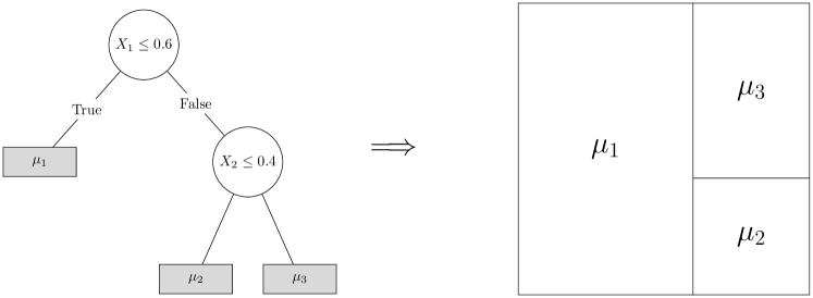
Figure 1: Schematic which shows how a decision tree induces a regression function. Associated to the decision tree on the left is a partition of $[0,1]^{2}$ with the function $g(x;\mathcal{T},\mathcal{M})$ returning $\mu_{1},\mu_{2}$, or $\mu_{3}$.

A problem with methods based on decision trees is that realizations of $r\sim\textnormal{BART}(\pi_{\mathcal{T}},\pi_{\mathcal{M}})$ will not be continuous in $x$. This is particularly problematic for density estimation, as we generally prefer estimates of the density to be continuous. A smooth variant of BART called soft BART (SBART) was introduced by Linero and Yang, (2018). This takes the tree $\mathcal{T}_{m}$ to be a smooth decision tree, where observations are assigned a weight $\varphi_{m\ell}(x)$ to leaf node $\ell$ of tree $m$. As a point of comparison, non-soft decision trees use the weights $\varphi_{m\ell}(x)=\prod_{b\in\mathcal{A}_{m\ell}}I(x_{j_{b}}\leq C_{b})^{1-R_{b}}\ I(x_{j_{b}}>C_{b})^{R_{b}},$ where $\mathcal{A}_{m\ell}$ denotes the collection of branches which are ancestors of leaf $\ell$ of tree $m$, $j_{b}$ denotes the coordinate along which $b$ splits, $C_{b}$ denotes the cutpoint of branch $b$, and $R_{b}$ is the indicator that the path from the root to the leaf goes right at $b$. A soft decision tree instead takes

$$\varphi_{m\ell}(x)=\prod_{b\in\mathcal{A}_{m\ell}}\psi(x;C_{b},\tau_{b})^{1-R_{b}}\ \{1-\psi(x;C_{b},\tau_{b})\}^{R_{b}},$$

where $\psi(x;c,\tau)$ is the cumulative distribution function of a location-scale family with location $c$ and scale $\tau$. If $\psi(x)=I(x\leq 0)$ (or, equivalently, as $\tau\to 0)$ we get a standard decision tree. If we instead take $\psi(x)$ to be a smooth function then $r(y,x)$ will also be smooth. The parameter $\tau$ is analogous to a bandwidth parameter, with larger values of $\tau$ giving smoother functions. Like Linero and Yang, (2018) we will take $\psi(x)=(1+e^{-x})^{-1}$ and use tree-specific bandwidths $\tau_{m}$. We write $r\sim\textnormal{SBART}(\pi_{\mathcal{T}},\pi_{\mathcal{M}})$ to denote that $r$ has an SBART prior, where $\pi_{\mathcal{T}}$ is now a prior over the soft trees $\mathcal{T}_{m}$.

For completeness, we describe the prior over the tree structures we will use. We assume that each coordinate $x_{j}$ of the predictors has been scaled to lie in $[0,1$]. This can be done, for example, by applying the empirical quantile transform to a subset of the observed values for each predictor and then interpolating the remaining values. A tree $\mathcal{T}_{m}$ is sampled in the following steps.

1. Initialize $\mathcal{T}_{m}$ with an single node of depth $D_{m}=0$.

2. For all nodes of depth $D_{m}$, make that node a branch node, with a left and right child of depth $D_{m}+1$, with probability $\alpha(1+D_{m})^{-\beta}$; otherwise, make the node a leaf node.

3. For all branch nodes $b$ of depth $D_{m}$, sample the splitting coordinate $j_{b}\sim\textnormal{Categorical}(s)$ and a splitting point $C_{b}\sim\textnormal{Uniform}(L_{j_{b}},U_{j_{b}})$ where $\prod_{j=1}^{P}[L_{j},U_{j}]$ denotes the hyperrectangle of $x$-values which lead to node $b$.

4. If all nodes of depth $D_{m}$ are leaf nodes, terminate; otherwise, set $D_{m}\leftarrow D_{m}+1$ and return to Step 2.

The distribution of the splitting coordinate $j_{b}\sim\textnormal{Categorical}(s)$ determines how relevant a-priori we expect predictor to be; for example, if $s_{1}=0.99$ we expect most splitting rules to use $x_{1}$, whereas if $s_{1}=10^{-10}$ we expect none of the splitting rules to use $x_{1}$. Linero, (2018) took advantage of this fact to perform automatic relevant determination (Neal,, 1995) for BART models by using a sparsity-inducing Dirichlet prior $s\sim\textnormal{Dirichlet}(a/P,\ldots,a/P)$ for some $a\ll P$. We also use this prior for the splitting proportion, which will allow us to perform automatic relevance determination in the density regression setting. This prior is crucial for proving that the posterior adapts to the presence of irrelevant predictors.

2.2 The Soft BART Density Sampler

Our modeling strategy is based on the representation (1) $f(y\mid x)\propto h(y\mid x,\theta)\ \Phi\{r(y,x)\}$ where $\Phi(\mu)$ is a continuous, non-negative, monotonically increasing link function. Taking $r(y,x)=\Phi^{-1}\{f(y\mid x)/h(y\mid x,\theta)\}$ we see that (1) is valid whenever $h(y\mid x,\theta)$ and $f(y\mid x)$ have the same support for all $x$.

A naive approach is to set $r(y,x)\sim\textnormal{BART}(\pi_{\mathcal{T}},\pi_{\mathcal{M}})$. This specification has two problems. First, $r(y,x)$ will not be smooth in $y$ so that draws from the prior and posterior of $f(y\mid x)$ will also not be smooth. The smoothness problem can be addressed by setting $r(y,x)\sim\textnormal{SBART}(\pi_{\mathcal{T}},\pi_{\mathcal{M}})$ instead. It is this model that we study the theoretical properties of in Section 4.

Setting $r(y,x)\sim\textnormal{SBART}(\pi_{\mathcal{T}},\pi_{\mathcal{M}})$ is still naive because of the way in which BART shrinks $r(y,x)$ towards additive models such that $r(y,x)=\sum_{v=1}^{V}r_{v}(y,x)$ where each $r_{v}(y,x)$ depends on a small subset of the coordinates of $(y,x)$ (Linero and Yang,, 2018; Rockova and van der Pas,, 2017). In the regression setting, we often expect that an underlying regression function will have exactly this form; in the case of sparse additive models (Ravikumar et al.,, 2007) for example, each $r_{v}(y,x)$ would depend on exactly one coordinate. This type of shrinkage-towards-additivity is not appropriate for conditional density estimation due to the distinguished nature of the response $y$; we instead want the predictors to interact with $y$.

To see why we want to force interactions with $y$, consider the strictly additive function $r(y,x)=r_{Y}(y)+\sum_{p=1}^{P}r_{p}(x_{p})$. If we take $\Phi(\mu)=e^{\mu},$ a massive cancellation occurs in (1) and the model reduces to $f(y\mid x)=h(y\mid x,\theta)\ \Phi\{r_{Y}(y)\}/\int h(\widetilde{y}\mid x,\theta)\ \Phi\{r_{Y}(\widetilde{y})\}\ d\widetilde{y}$, effectively eliminating the predictors from the model. More generally, any trees which do not split on $Y_{i}$ will have no effect on $f(y\mid x)$. While exact cancellation is unique to the exponential link, it occurs in an approximate form for the logistic link as well. At the other extreme, SBART-DS uses a prior which favors utilizing a small number of coordinates. If $y$ is eliminated, massive cancellation occurs irrespective of the link function, and gives $f(y\mid x)=h(y\mid x,\theta)$. Combined with a Dirichlet prior for $s$, this approach encodes prior information that $f(y\mid x)$ is exactly equal to $h(y\mid x,\theta)$ with high probability.

2.3 Targeted Smoothing via Random Basis Function Expansions

We use the “targeted smoothing” approach of Starling et al., (2018) to overcome the problems of the naive SBART-DS prior. They set $r(y,x)=\gamma+\sum_{m=1}^{M}g(y;x,\mathcal{T}_{m},\mathcal{M}_{m})$ where each leaf node is associated with a Gaussian process; that is, for fixed $x$, we have $g(y;x;\mathcal{T}_{m},\mathcal{M}_{m})\sim\textnormal{GP}\{0,\Sigma(\cdot,\cdot)\}$ where $\textnormal{GP}\{0,\Sigma(\cdot,\cdot)\}$ denotes a mean-$0$ Gaussian process with covariance function $\Sigma(y,y^{\prime})$.

Starling et al., (2018) consider the case where the number of unique values $y$ takes, $N_{y}$, is small. When $N_{y}$ is large this is no longer practical due to the need to store and invert an $N_{y}\times N_{y}$ matrix for all $m$ trees. For SBART-DS we cannot guarantee that this is the case. Instead, we set $r(y,x)=\gamma+\sum_{m=1}^{M}\mathcal{B}_{m}(y)\ g(x;\mathcal{T}_{m},\mathcal{M}_{m})$ where each $\mathcal{B}_{m}$ is a random basis function.

To construct our approximation, consider the case where $\mathcal{T}_{m}$ us a non-soft decision tree. For fixed $x$ we can write $r(y,x)=\gamma+M^{-1/2}\sum_{m=1}^{M}\mu_{m}\ \mathcal{B}_{m}(y)$ where the $\mu_{m}$’s are iid $\textnormal{Normal}(0,\sigma_{\mu}^{2})$ random variables. Under mild regularity conditions on the distribution of the $\mathcal{B}_{m}$’s, as $M\to\infty$ a functional central limit theorem will hold and this will converge weakly to a Gaussian process with mean $\gamma$ and covariance function

$$\Sigma(y,y^{\prime})=\sigma_{\mu}^{2}\mathbb{E}\{\mathcal{B}_{1}(y)\ \mathcal{B}_{1}(y^{\prime})\}.$$ (2)

This is the same as the distribution of $r(\cdot,x)$ used by Starling et al., (2018). Rather than directly choose the basis functions $\mathcal{B}_{m}$, we specify $\Sigma(y,y^{\prime})$ and derive a distribution for $\mathcal{B}_{m}$ which matches (2). We make use of the following proposition, which follows from Bochner’s Theorem, and is stated for completeness.

Proposition 1.

Let $\Sigma(y,y^{\prime})=\sigma_{\mu}^{2}\delta(y-y^{\prime})$ be a shift-invariant kernel with $\delta(0)=1$. Then there exists a distribution $P(d\omega)$ such that $\Sigma(y,y^{\prime})=\sigma_{\mu}^{2}\mathbb{E}\{2\cos(\omega y+b)\cos(\omega y^{\prime}+b)\}$ where $\omega\sim P(d\omega)$ and $b\sim\textnormal{Uniform}(0,2\pi)$. Moreover, $\delta(\cdot)$ is the characteristic function of $P(d\omega)$, i.e., $\delta(t)=\int\exp\{i\omega t\}\ P(d\omega)$.

The approach of using random Fourier features in this fashion was introduced by Rahimi and Recht, (2008). It follows from Proposition 1 that we can take $\mathcal{B}_{m}(y)=\sqrt{2}\cos(\omega_{m}y+b_{m})$ where $\omega_{m}\stackrel{{\scriptstyle\textnormal{iid}}}{{\sim}}P(d\omega)$ and $b_{m}\stackrel{{\scriptstyle\textnormal{iid}}}{{\sim}}\textnormal{Uniform}(0,2\pi)$. We list some possible choices below.

• $\omega_{m}\sim\textnormal{Normal}(0,\rho^{-2})$ corresponds to the squared exponential covariance $\Sigma(y,y^{\prime})=\sigma_{\mu}^{2}\exp\{-(y-y^{\prime})^{2}/(2\rho^{2})\}$.

• Setting $\omega_{m}\sim t_{\nu}$ with location $0$ and scale $\rho^{-1}$ gives the Matern kernel

  $$\Sigma(y,y^{\prime})=\sigma_{\mu}^{2}\frac{1}{2^{v/2-1}\Gamma(v/2)}\left(\frac{\sqrt{v}|y-y^{\prime}|}{\rho}\right)^{v/2}K_{v/2}\left(\frac{\sqrt{v}|y-y^{\prime}|}{\rho}\right)$$

  where $K_{\nu}(\cdot)$ is a modified Bessel function of the second kind. The exponential kernel $\Sigma(y,y^{\prime})=\sigma_{\mu}^{2}\exp\{-|y-y^{\prime}|/\rho\}$ is a special case ($v=1$).

• In general, $P(d\omega)=p(\omega)\ d\omega$ can be obtained from the inversion formula $p(\omega)=\frac{1}{2\pi}\int e^{-it\omega}\ \delta(t)\ dt$. For example, inverting a Cauchy kernel $\delta(t)=\{1+t^{2}/\rho^{2}\}^{-1}$ shows that we can get a Cauchy kernel by sampling from the Laplace distribution $p(\omega)=\frac{\rho}{2}e^{-\rho|\omega|}$.

2.4 Shrinking Towards the Base Model

A desirable feature of mixture models is the ability to center the prior on a parametric submodel. Consider the infinite mixture $\sum_{k=1}^{\infty}\pi_{k}(x)\ h(y\mid x,\theta_{k})$. If we choose the prior so that $\pi_{1}(x)\approx 1$ with high probability, then we are encoding prior knowledge that $h(y\mid x,\theta)$ is itself highly likely to give an adequate representation of the data. For models based on Dirichlet process mixtures $f(x,y)=\int h(x,y\mid\theta)\ F(d\theta)$ with $F\sim\textnormal{Dirichlet}(\alpha,F_{0}$), for example, this can be accomplished by choosing a prior which shrinks $\alpha$ heavily towards $0$. We can accomplish a similar goal with SBART-DS. Note that if $\Phi\{r(y,x)\}$ is a constant then it can be canceled in (1) so that $f(y\mid x)$ reverts to $h(y\mid x,\theta)$. One approach is to use a prior which encourages $\sigma_{\mu}^{2}$ to be close to $0$, so that $\Phi\{r(y,x)\}\approx\Phi(\gamma)$, which is constant. A second approach is to use a prior which encourages $\gamma$ to be large and positive, so that $\Phi\{r(y,x)\}\approx 1$.

To quantify these observations, let $\Delta_{x}=\sup_{y}|\sum_{m=1}^{M}\mathcal{B}_{m}(y)\ g(x;\mathcal{T}_{m},\mathcal{M}_{m})/\sigma_{\mu}|$, let $\Phi(\mu)$ satisfy Condition L in Section 4, and let $H(f,g)$ and $K(f,g)$ denote the Hellinger distance and Kullback-Leibler divergence respectively. Note that the distribution of $\Delta_{x}$ is free of $\sigma_{\mu}$. An application of Lemma 1 shows that $H(f,g)=O_{p}(\sigma_{\mu})$ and $K(f,g)=O_{p}(\sigma_{\mu}^{2})$. It can further be shown that $K\{h(y\mid x,\theta),f(y\mid x)\}\leq-\log\Phi(\gamma-\sigma_{\mu}\Delta_{x})$, so that choosing a prior which makes $\gamma-\sigma_{\mu}\Delta_{x}$ large will also make the Kullback-Leibler divergence small; this can be accomplished by centering $\gamma$ far away from $0$. More quantitative results might be obtained from concentration inequalities for $\Delta_{x}$, but we do not pursue this here.

2.5 Default Prior Specification

In our illustrations we use the following default prior specification. Following Chipman et al., (2010), we fix the parameters $\alpha=0.95$ and $\beta=2$ in the prior for $\pi_{\mathcal{T}}$ and set $\mu_{m\ell}\sim\textnormal{Normal}(0,\sigma_{\mu}^{2}/M)$. We fix $M=50$; in general, we recommend trying multiple values of $M$. We set $\sigma_{\mu}\sim\text{Half-Cauchy}(0,1.5)$ to learn an appropriate value of $\sigma_{\mu}$ from the data. By having mass near $\sigma_{\mu}=0$, this also allows us to revert to the base model $h(y\mid x,\theta)$. To induce further shrinkage to the base model, we set $\gamma\sim\textnormal{Normal}(1,1)$. This has the additional benefit of making the prior prefer models for which $\Phi\{r(y,x)\}$ is close to $1$, which reduces the number of latent variables we need to introduce when fitting the model by MCMC (see Section 3). We use tree-specific bandwidths $\tau_{m}$ which are exponentially distributed with mean $0.1$. To perform variable selection we specify $s\sim\textnormal{Dirichlet}(a/P,\ldots,a/P)$ and use a hyperprior $a/(a+P)\sim\textnormal{Beta}(0.5,1)$.

For targeted smoothing, we approximate the squared exponential kernel by setting $\omega_{m}\sim\textnormal{Normal}(0,\rho^{-2})$. We set $\rho^{2}\sim\textnormal{Gam}(\alpha_{\rho},\beta_{\rho})$ to allow the length scale to be learned from the data. As a default, we set $\alpha_{\rho}=1$ and $\beta_{\rho}=\pi^{2}/4$ after scaling the $Y_{i}$’s to have unit variance. This choice is based on the expected number of times a Gaussian process with length-scale $\rho$ is expected to cross $0$ on the interval $(-1,1)$: the expected number of crossings is $2/(\pi\rho)$ so that if $\rho^{2}=4/\pi^{2}$ the expected number of crossings is $1$. Smaller values of $\rho^{2}$ correspond to more wiggly functions. Because our prior has positive density at $0$, setting $\alpha_{\rho}=1$ allows for the possibility that the function is very wiggly while defaulting to the prior belief that it is not.

We choose the base model to be a Gaussian linear model with $h(y\mid x,\theta)=\varphi(y\mid\alpha_{\theta}+x^{\top}\beta_{\theta},\sigma_{\theta})$ where $\varphi(y\mid\mu,\sigma)$ is the density of a Gaussian random variable with mean $\mu$ and variance $\sigma^{2}$. In our examples we set $\pi(\alpha_{\theta},\beta_{\theta},\sigma_{\theta})\propto\sigma_{\theta}^{-1}$. We can also shrink towards a semiparametric Gaussian model by setting $h(y\mid x,\theta)=\varphi\{y\mid r_{\theta}(x),\sigma_{\theta}\}$ where $r_{\theta}(x)\sim\textnormal{SBART}(\pi_{\mathcal{T}}^{\theta},\pi_{\mathcal{M}}^{\theta})$ and the default prior of Linero and Yang, (2018) is specified for $(\pi_{\mathcal{T}}^{\theta},\pi_{\mathcal{M}}^{\theta})$.

3 Posterior Computation

3.1 Rejection Sampling Data Augmentation

We use a two-layer data augmentation scheme which removes both the intractable integral in the denominator of (1) and the link function $\Phi(\mu)$ from the likelihood. Our approach is based on the following method for sampling from $f(y\mid x)$.

Proposition 2.

Suppose that we sample $Y_{1},Y_{2},Y_{3},\ldots\stackrel{{\scriptstyle\textnormal{iid}}}{{\sim}}h(y\mid x,\theta)$ and sample $A_{j}\stackrel{{\scriptstyle\textnormal{indep}}}{{\sim}}\textnormal{Bernoulli}[\Phi\{r(Y_{j},x)\}]$. Let $Z$ denote the $Y_{j}$ associated with the smallest index $J+1$ for which $A_{J+1}=1$. Then conditional on $\{J,A_{j}:1\leq j\leq J+1\}$, $Z$ is a draw from $f(y\mid x)\propto h(y\mid x,\theta)\Phi\{r(y,x)\}$ and $Y_{1},\ldots,Y_{J}$ are draws from $\bar{f}(y\mid x)\propto h(y\mid x,\theta)[1-\Phi\{r(y,x)\}]$.

We make use of Proposition 2 by augmenting the latent index $J$ and the sequence of rejected points. Associated to each observation $Y_{i}=Y_{i0}$ we sample $Y_{ij}\sim h(y\mid X_{i},\theta)$ and $A_{ij}\sim\textnormal{Bernoulli}[\Phi(r(Y_{ij},X_{i})]$ until we reach the first iteration $J_{i}+1$ such that $A_{i(J_{i}+1)}=1$. We then work with the augmented state $\{Y_{ij}:1\leq i\leq N,0\leq j\leq J_{i}\}$, which has likelihood

$$\prod_{i=1}^{N}\prod_{j=0}^{J_{i}}h(Y_{ij}\mid X_{i},\theta)\times\prod_{i=1}^{N}\left(\Phi\{r(Y_{i0},X_{i})\}\prod_{j=1}^{J_{i}}[1-\Phi\{r(Y_{ij},X_{i})\}]\right).$$ (3)

For more details on the derivation of this expression, see Rao et al., (2016), who consider the GP-DS model. At this stage Rao et al., (2016) propose the use of Hamiltonian Monte Carlo to sample from the posterior distribution. This is not an option for us, as the $\mathcal{T}_{m}$’s are discrete parameters.

3.2 Bayesian Backfitting for Probit, Logit, and Student’s $t_{\nu}$ Links

We now apply data augmentation strategy of Albert and Chib, (1993). Suppose that $\Phi(\mu)$ is cdf of either the probit, logit, or Student’s $t_{\nu}$ link. We can then associate to each $A_{ij}$ from Section 3.1 a random variable

$$Z_{ij}=r(Y_{ij},X_{i})+\epsilon_{ij},\qquad\epsilon_{ij}\sim\textnormal{Normal}(0,\lambda_{ij}^{-1}),\qquad\lambda_{ij}\sim g(\lambda).$$

Setting $A_{ij}=I(Z_{ij}\geq 0)$ recovers the $\textnormal{Bernoulli}[\Phi\{r(Y_{ij},X_{i})\}]$ model. This model captures the three links we consider:

• For the probit link, $\lambda_{ij}^{-1}$ has a point-mass distribution at $1$.

• When $\Phi(\mu)=T_{\nu}(\mu)$ is the Student’s $t$ link with $\nu$ degrees of freedom, $\lambda_{ij}\sim\textnormal{Gam}(\nu/2,\nu/2)$.

• When $\Phi(\mu)=(1+e^{-\mu})^{-1}$ is the logistic link, $\lambda_{ij}^{-1/2}/2$ has a Kolmogorov-Smirnov distribution (Holmes and Held,, 2006).

Compared to (3), introducing the latent variables $(Z_{ij},\lambda_{ij})$ leads to a more tractable likelihood:

$$\prod_{i=1}^{N}\prod_{j=0}^{J_{i}}h(Y_{ij}\mid X_{i},\theta)\times\textnormal{Normal}\{Z_{ij}\mid r(Y_{ij},X_{i}),\lambda_{ij}^{-1}\}\times g(\lambda_{ij}).$$ (4)

After reaching expression (4) we can apply a Bayesian backfitting algorithm to update $r(y,x)$. While the Bayesian backfitting algorithm originally proposed by Chipman et al., (2010) does not account for heteroskedasticity in the $Z_{ij}$’s, several recent works have shown how to accommodate this (Bleich and Kapelner,, 2014; Pratola et al.,, 2017; Linero et al.,, 2018). Consider the prior $\gamma\sim\textnormal{Normal}(\mu_{\gamma},\lambda_{\gamma}^{-1})$ and let $R_{ij}=Z_{ij}-\gamma-\sum_{m\neq k}\mathcal{B}_{m}(Y_{ij})\ g(X_{i};\mathcal{T}_{m},\mathcal{M}_{m})$. When updating $\mathcal{T}_{k}$ it suffices to consider the backfit model

$$R_{ij}=\mathcal{B}_{k}(Y_{ij})\ g(X_{i};\mathcal{T}_{k},\mathcal{M}_{k})+\epsilon_{ij},\qquad\epsilon_{ij}\sim\textnormal{Normal}(0,\lambda_{ij}^{-1}),$$ (5)

where recall that $\varphi_{k\ell}(X_{i})$ is the weight associated to leaf $\ell$ of tree $k$ at $X_{i}$. Let $\varphi_{k}(X_{i})$ be a vector with $\ell^{\text{th}}$ entry $\varphi_{k\ell}(X_{i})$. Then we can rewrite (5) as $R_{ij}=\mathcal{B}_{k}(Y_{ij})\ \varphi_{k}(X_{i})^{\top}\mu_{k}+\epsilon_{ij}$ or, in multivariate form, $\bm{R}\sim\textnormal{Normal}(\mathcal{B}_{k}\mu,\Lambda^{-1})$ where the rows of $\mathcal{B}_{k}$ correspond to $\mathcal{B}_{k}(Y_{ij})\varphi_{k}(X_{i})^{\top}$ and $\Lambda$ is diagonal with entries $\lambda_{ij}$. If $\mu_{k}\sim\textnormal{Normal}(0,\lambda_{\mu}^{-1})$ where $\lambda_{\mu}=M/\sigma_{\mu}^{2}$ then it follows from standard properties of the multivariate Gaussian distribution that

$$\bm{R}\sim\textnormal{Normal}(0,\Lambda^{-1}+\mathcal{B}_{k}\mathcal{B}_{k}^{\top}/\lambda_{\mu})]$$ and (6)

$${}[\mu_{k}\mid\bm{R}]\sim\textnormal{Normal}(V\mathcal{B}_{k}^{\top}\Lambda\bm{R},V) \text{where }V=(\mathcal{B}_{k}^{\top}\Lambda\mathcal{B}_{k}+\lambda_{\mu}\textnormal{I})^{-1}.$$

After applying the Woodbury matrix identity and the matrix determinant lemma (Brookes,, 2011, matrix identities), the likelihood of $\mathcal{T}_{k}$ after integrating out $\mu_{k}$ is given by

$$(2\pi)^{-N/2}\prod_{i=1}^{N}\lambda_{i}^{1/2}\det(\textnormal{I}+\mathcal{B}_{k}^{\top}\Lambda\mathcal{B}_{k}/\lambda_{\mu})\ \exp\left[-\frac{1}{2}\left\{\bm{R}^{\top}\Lambda\bm{R}-\delta^{\top}(\textnormal{I}+\mathcal{B}_{k}^{\top}\Lambda\mathcal{B}_{k}/\lambda_{\mu})^{-1}\delta\right\}\right]$$ (7)

where $\delta=\mathcal{B}_{k}^{\top}\Lambda\bm{R}$. The value of (7) is that it avoids taking the determinant of and inverting the $N\times N$ matrix $\Lambda^{-1}+\mathcal{B}_{k}\mathcal{B}_{k}^{\top}/\lambda_{\mu}$. The marginal likelihood $L_{k}(\mathcal{T},\mathcal{B})$ given by (7) is used to update both the tree topology $\mathcal{T}_{k}$ and the random basis function $\mathcal{B}_{k}(y)$ using Metropolis-Hastings.

Our final MCMC scheme is summarized in Algorithm 1, which calls Algorithm 2 to update $(\mathcal{T}_{k},\mathcal{B}_{k},\mathcal{M}_{k})$. The Markov transition function $Q(\mathcal{T}_{k}\to\mathcal{T}^{\prime})$ used to propose new tree topologies is a mixture of the BIRTH, DEATH, and CHANGE proposals described by Chipman et al., (1998) and a PRIOR proposal which samples $\mathcal{T}^{\prime}$ from the prior.

Algorithm 1 An iteration of the data augmentation algorithm for SBART-DS

1. For $i=1,\ldots,N$, set $Y_{i0}=Y_{i}$ and sample $Y_{i1},Y_{i2},\ldots\sim h(y\mid X_{i},\theta)$ and $A_{i1},A_{i2},\ldots\sim\textnormal{Bernoulli}[\Phi\{r(Y_{ij},X_{i})\}]$ until $A_{i(J_{i}+1)}=1$. Retain the samples $Y_{i0},\ldots,Y_{iJ_{i}}$.

2. Make an update to $\theta$ which leaves the full conditional $\pi(\theta\mid-)\propto\pi(\theta)\prod_{i,j}h(Y_{ij}\mid X_{i},\theta)$ invariant.

3. Sample $Z_{ij}\sim f(z\mid\mu_{ij})$ truncated to $(0,\infty)$ for $j=0$ and $(-\infty,0)$ for $j>0$ where $\mu_{ij}=r(Y_{ij},X_{i})$ and $f(z\mid\mu_{ij})$ is a normal, logistic, or Student’s $t_{\nu}$ distribution with location $\mu_{ij}$ and scale $1$ for the probit, logit, and $T_{\nu}$ links respectively.

4. Sample $\lambda_{ij}$ from its full conditional given $Z_{ij}$ for all $1\leq i\leq N$ and $0\leq j\leq J_{i}$.

   • For the probit link, $\lambda_{ij}\equiv 1$.

   • For the Student’s $t_{\nu}$ link, $\lambda_{ij}\sim\text{Gam}\{(\nu+1)/2,(\nu+[Z_{ij}-r(Y_{ij},X_{i})]^{2})/2\}.$

   • For the logit link, sample $\lambda_{ij}^{-1}$ using the rejection sampling algorithm of Holmes and Held, (2006).

5. For $m=1,\ldots,M$ update $(\mathcal{T}_{m},\mathcal{M}_{m},\mathcal{B}_{m})$ using the Metropolis-Hastings algorithm given in Algorithm 2.

Algorithm 2 Metropolis-Hastings update for $(\mathcal{T}_{k},\mathcal{M}_{k},\mathcal{B}_{k})$

1. Compute $\bm{R}$ as in (5).

2. Propose a tree $\mathcal{T}^{\prime}$ from a Markov transition kernel $Q(\mathcal{T}_{k}\to\mathcal{T}^{\prime})$.

3. Set $\mathcal{T}_{k}=\mathcal{T}^{\prime}$ with probability

   $$\min\left\{\frac{\pi_{\mathcal{T}}(\mathcal{T}^{\prime})\ L_{k}(\mathcal{T}^{\prime},\mathcal{B}_{k})\ Q(\mathcal{T}^{\prime}\to\mathcal{T}_{k})}{\pi_{\mathcal{T}}(\mathcal{T}_{k})\ L_{k}(\mathcal{T}_{k},\mathcal{B}_{k})\ Q(\mathcal{T}_{k}\to\mathcal{T}^{\prime})},1\right\}.$$

   Otherwise, do not change $\mathcal{T}_{k}$.

4. Sample a basis function $\mathcal{B}^{\prime}(y)=\sqrt{2}\cos(\omega^{\prime}y+b^{\prime})$ by sampling $\omega^{\prime}\sim P(d\omega)$ and $b^{\prime}\sim\textnormal{Uniform}(0,2\pi)$. Then set $\mathcal{B}_{k}=\mathcal{B}^{\prime}$ with probability

   $$\min\left\{\frac{L_{k}(\mathcal{T}_{k},\mathcal{B}^{\prime})}{L_{k}(\mathcal{T}_{k},\mathcal{B}_{k})},1\right\}.$$

   Otherwise, do not change $\mathcal{B}_{k}$.

5. Sample $\mu_{k}\sim\textnormal{Normal}(V\mathcal{B}_{k}^{\top}\Lambda\bm{R},V)$ where $V=(\mathcal{B}_{k}^{\top}\Lambda\mathcal{B}_{k}+\textnormal{I}/\lambda_{\mu})^{-1}$ and $\lambda_{\mu}=M/\sigma_{\mu}^{2}$.

4 Theoretical Results

We show that SBART-DS attains close to the minimax-optimal concentration rate for $(P+1)$-dimensional functions $r(y,x)$ in the high-dimensional sparse setting. All proofs are deferred to the appendix. We consider the case where $r(y,x)$ depends on only $D$ coordinates of $(y,x)^{\top}$ where the relevant subset is unknown and must be learned from the data. Following Pati et al., (2013) we study concentration with respect to the integrated Hellinger distance. Let $H(f,f_{0})=\{\int(\sqrt{f_{0}(y\mid x})-\sqrt{f(y\mid x})^{2}\ dy\ F_{X}(dx)\}^{1/2}$ denote the $F_{X}$-integrated Hellinger distance between $f_{0}(y\mid x)$ and $f(y\mid x)$. The covariates $X_{i}$ are assumed to be iid from $F_{X}$, which is not assumed to be known. We similarly define an $F_{X}$-integrated Kullback-Leibler neighborhood. Define $K(f_{0},f)=\int f_{0}\log\frac{f_{0}}{f}\ dy\ dF_{X}$ and $V(f_{0},f)=\int f_{0}\left(\log\frac{f_{0}}{f}\right)^{2}\ dy\ dF_{X}$. Then the integrated Kullback-Leibler neighborhood is given by $K(\epsilon)=\left\{f:K(f_{0},f)\leq\epsilon^{2}\ \text{and }V(f_{0},f)\leq\epsilon^{2}\right\}.$ Let $\mathcal{D}_{n}$ denote the data $\{X_{i},Y_{i}:i=1,\ldots,n\}$ and let $\Pi$ denote a prior distribution on $r$ and additional hyperparameters. We say that the posterior has a convergence rate of at least $\epsilon_{n}$ if there exists a constant $C>0$ such that $\Pi\{H(f_{r},f_{0})\geq C\epsilon_{n}\mid\mathcal{D}_{n}\}\to 0$ in probability. To simplify the theoretical results, we assume that $X_{i}$ and $Y_{i}$ take values in $[0,1]^{P+1}$. We additionally make the following assumptions about the true data generating process $F_{0}$.

Condition F (on $F_{0}$):

The true conditional density $f_{0}(y\mid x)$ can be written as $f_{r_{0}}(y\mid x)$ for some $r_{0}\in C^{\alpha,R}([0,1]^{P+1})$ where $C^{\alpha,R}([0,1])$ is the ball of radius $R$ in the space of $\alpha$-Hölder smooth functions on $[0,1]^{P+1}$, where $f_{r}(y\mid x)$ is defined as

$$f_{r}(y\mid x)=\frac{h(y)\ \Phi\{r(y,x)\}}{\int h(\widetilde{y})\ \Phi\{r(\widetilde{y},x)\}\ d\widetilde{y}}$$

for some density $h(y)$ on $[0,1]$. Additionally, we can write $r_{0}(y,x)=\widetilde{r}(y,x_{\mathcal{S}})$ where $x_{\mathcal{S}}=\{x_{j}:j\in\mathcal{S}\}$ and $\mathcal{S}$ is a subset of $\{1,\ldots,P\}$ of cardinality $D-1$. That is, $r_{0}(y,x)$ depends on at most $D$ coordinates of $(y,x)^{\top}$. The number of predictors $P\equiv P_{n}$ depends on $n$ but is such that $\log(P+1)\leq C_{\eta}n^{\eta}$ for some $\eta\in(0,1)$.

Remark 1.

For simplicity, we consider $\widetilde{r}$ and $\mathcal{S}$ to be independent of $n$; in particular, we do not consider $D$ diverging with $n$. There exists some $r_{0}$ such that $f_{0}=f_{r_{0}}$ by taking $r_{0}(y\mid x)=\Phi^{-1}\{f_{0}(y\mid x)/h(y)\}$, provided that $h(y)$ and $f_{0}(y\mid x)$ have common support. When $h(y)=1$, the assumption that $r_{0}$ is continuous on $[0,1]^{P+1}$ implies that $C^{-1}\leq f_{0}(y\mid x)\leq C$ for some constant $C$, i.e., $f_{0}(y\mid x)$ is bounded and bounded away from $0$.

Condition L (on $\Phi)$:

The link function $\Phi(\mu)$ is strictly increasing and is the cumulative distribution function of a random variable $Z$ which is symmetric about $0$ and has density $\phi(\mu)$ satisfying $\phi(\mu)/\Phi(\mu)\leq\mathcal{K}$ for all $\mu$ and some constant $\mathcal{K}$.

Remark 2.

We show in the appendix that Condition L holds for the logit ($\mathcal{K}=1$) and $t_{\nu}$ ($\mathcal{K}=\sqrt{\nu}$) links, but fails for the probit link.

Condition P (on $\Pi$):

The function $r$ is given an $\text{SBART}(\pi_{\mathcal{T}},\pi_{\mathcal{M}})$ prior with $M$ trees, conditional on $(\pi_{\mathcal{T}},\pi_{\mathcal{M}},M)$. Additionally, the prior $\Pi$ satisfies the following conditions.

1. There exists positive constants $(C_{M1},C_{M2})$ such that the prior on the number of trees $M$ in the ensemble is $\Pi(M=t)=C_{M1}\exp\{-C_{M2}t\log t\}$.

2. A single bandwidth $\tau_{m}\equiv\tau$ is used and its prior satisfies $\Pi(\tau\geq x)\leq C_{\tau 1}\exp(-x^{C_{\tau 2}})$ and $\Pi(\tau^{-1}\geq x)\leq C_{\tau 3}\exp(-x^{C_{\tau 4}})$ for some positive constants $C_{\tau 1},\ldots,C_{\tau 4}$ for all sufficiently large $x$, with $C_{\tau 2},C_{\tau 4}<1$. Moreover, the density of $\tau^{-1}$ satisfies $\pi_{\tau^{-1}}(x)\geq C_{\tau 5}e^{-C_{\tau 6}x}$ for large enough $x$ and some positive constants $C_{\tau 5}$ and $C_{\tau 6}$.

3. The prior on the splitting proportions is $s\sim\text{Dirichlet}(a/P^{\xi},\ldots,a/P^{\xi})$ for some $\xi>1$ and $a>0$.

4. The $\mu_{m\ell}$’s are iid from a density $\pi_{\mu}(\mu)$ such that $\pi_{\mu}(\mu)\geq C_{\mu 1}e^{-C_{\mu 2}|\mu|}$ for some coefficients $C_{\mu 1},C_{\mu 2}$. Additionally, there exists constants $C_{\mu 3},C_{\mu 4}$ such that $\Pi(|\mu_{m\ell}|\geq t)\leq C_{\mu 3}\exp\{-t^{C_{\mu 4}}\}$ for all $t$.

5. Let $D_{m}$ denote the depth of tree $\mathcal{T}_{m}$. Then $\Pi(D_{m}=k)>0$ for all $k=0,1,\ldots,2D$ and $\Pi(D_{m}>d_{0})=0$ for some $d_{0}\geq D$.

6. The gating function $\psi:\mathbb{R}\to[0,1]$ of the SBART prior is such that $\sup_{x}|\psi^{\prime}(x)|<\infty$ and the function $\rho(x)=\psi(x)\{1-\psi(x)\}$ is such that $\int\rho(x)\ dx>0$, $\int|x|^{m}\rho(x)\ dx<\infty$ for all integers $m\geq 0$, and $\rho(x)$ can be analytically extended to some strip $\{z:|\Im(z)|\leq U\}$ in the complex plane.

Remark 3.

Conditions other than Condition P might also be used. Recent work of Rockova and van der Pas, (2017), for example, studies concentration results for BART using different sets of conditions, and the conditions overall are weaker than the conditions presented here. A downside of these results is they apply only when non-smooth decision trees are used, which induces non-smooth densities. Condition P2 holds when $\tau$ is given an inverse-gamma prior truncated from above, while Condition P4 holds when the $\mu_{m\ell}$’s are given a Laplace prior, although as noted by Linero and Yang, (2018) this could potentially be weakened to allow a Gaussian prior with a hyperprior on $\sigma_{\mu}$ (we do not pursue this here). Condition P6 holds for the logistic gating function $\psi(x)=\{1+\exp(-x)\}^{-1}$, which is used by default. Condition P5 holds if we truncate the prior of Chipman et al., (2010) at some large $d_{0}$, which is extremely unlikely to affect the MCMC in practice. Hence, satisfying P5 is not a practical concern. Condition P1 is problematic because BART implementations do not use a prior on $M$. In practice, we find that selecting $M$ by cross validation is more reliable than using a prior; we recommend either (i) using cross validation to select $M$ or (ii) fixing $M$ at a default value such as $M=200$ (recommended by Chipman et al.,, 2010) or $M=50$ (used here).

Theorem 1.

Suppose that Condition L, Condition F, and Condition P hold. Then there exists a positive constant $C$ such that $\Pi\{H(f_{0},f_{r})\geq C\epsilon_{n}\mid\mathcal{D}_{n}\}\to 0$ in probability, where $\epsilon_{n}=n^{-\alpha/(2\alpha+D)}(\log n)^{t}+\sqrt{\frac{D\log(P+1)}{n}}$ and $t=\alpha(D+1)/(2\alpha+D)$.

We prove Theorem 1 by checking (a)—(c) in Proposition 3, which are analogous to conditions of Ghosal et al., (2000).

Proposition 3.

Let $\Pi$ denote a prior for a conditional density $f(y\mid x)$ and let $\epsilon_{n}$ and $\bar{\epsilon}_{n}$ be sequences of positive numbers such that $\bar{\epsilon}_{n},\epsilon_{n}\to 0$, $n\epsilon_{n}^{2}\to\infty$, and $\epsilon_{n}\leq\bar{\epsilon}_{n}$. Let $N(\epsilon,\mathcal{F},H)$ denote the $\epsilon$-covering number of $\mathcal{F}$ with respect to $H$ (i.e., the number of balls of radius $\epsilon$ required to cover $\mathcal{F}$). Suppose that there exists positive constants $C,C_{N}$ such that for all sufficiently large $n$ there exist sets of conditional densities $\mathcal{F}_{n}$ satisfying the following conditions:

1. Entropy Bound: $\log N(\bar{\epsilon}_{n},\mathcal{F}_{n},H)\leq C_{N}n\bar{\epsilon}_{n}^{2}$.

2. Support Condition: $\Pi(\mathcal{F}_{n}^{c})\leq\exp\{-(C+4)n\epsilon_{n}^{2}\}$.

3. Prior Thickness: $\Pi\{f\in K(\epsilon_{n})\}\geq\exp(-Cn\epsilon_{n}^{2})$.

Then $\Pi\{H(f_{0},f)\geq A\bar{\epsilon}_{n}\mid\mathcal{D}_{n}\}\to 0$ in probability for some constant $A>0$.

The proof that our SBART prior satisfies these conditions is similar to the proof of Theorem 3.1 of van der Vaart and van Zanten, (2008), who established posterior convergence rates for density estimation using logistic Gaussian processes. We use a collection of results of Linero and Yang, (2018), who established results similar to (a)—(c) for a regression function $r\sim\text{SBART}(\pi_{\mathcal{T}},\pi_{\mathcal{M}})$ with respect to the supremum norm $\|r-r_{0}\|_{\infty}=\sup_{x,y}|r(y,x)-r_{0}(y,x)|$. We then use the following lemma, which links the supremum-norm neighborhoods of $r_{0}$ with the integrated Hellinger and Kullback-Leibler neighborhoods of $f_{0}$; this allows us to convert results about the $\|\cdot\|_{\infty}$-norm neighborhoods to results about the integrated neighborhoods. This lemma is similar to Lemma 3.1 of van der Vaart and van Zanten, (2008), but with exponential link $\Phi(\mu)=e^{\mu}$ replaced with a link satisfying Condition L.

Lemma 1.

Let $\Phi(\mu)$ be a link function satisfying Condition L. Then for any measurable functions $u,v:[0,1]^{P+1}\to\mathbb{R}$ we have the following:

• $H^{2}(f_{u},f_{v})\leq\mathcal{K}^{2}\|u-v\|_{\infty}^{2}\exp(\mathcal{K}\|u-v\|_{\infty})$;

• $K(f_{u},f_{v})\lesssim\|u-v\|_{\infty}^{2}\exp(\mathcal{K}\|u-v\|_{\infty})(1+2\mathcal{K}\|u-v\|_{\infty})$; and

• $V(f_{u},f_{v})\lesssim\|u-v\|_{\infty}^{2}\exp(\mathcal{K}\|u-v\|_{\infty})(1+2\mathcal{K}\|u-v\|_{\infty})^{2}$.

The expression $a\lesssim b$ here denotes that $a\leq Cb$ for some constant $C$ depending only on $\mathcal{K}$.

More generally, one expects that Theorem 1 can be improved to allow for additive decompositions $r_{0}(y,x)=\sum_{j=1}^{J}r_{0j}(y,x)$ where the $r_{0j}$’s are functions which are $D_{j}$-sparse and $\alpha_{j}$-Hölder continuous. Results in this framework (Linero and Yang,, 2018; Rockova and van der Pas,, 2017; Yang and Tokdar,, 2015) suggest that we should be able to obtain a rate $\epsilon_{n}=\sum_{j=1}^{J}n^{-\alpha_{j}/(2\alpha_{j}+D_{j})}\log(n)^{t_{j}}+\sqrt{n^{-1}D_{j}\log(P+1)}$, which is a substantial improvement on Theorem 1. One difficulty with extending these results is that Condition P2 only allows a single bandwidth, while different $\tau$’s will be optimal for different $\alpha_{j}$’s. Unlike the nonparametric regression setting, however, it is unclear how one would interpret the additivity assumption for SBART-DS. We leave examining the additive framework to future work.

5 Illustrations

5.1 Simulation Study

We now assess the performance of the SBART-DS using the simulation example described by Dunson et al., (2007). The response $Y_{i}$ is sampled from a mixture model

$$Y_{i}\sim e^{-2x}\text{Normal}(x,0.1^{2})+(1-e^{-2x})\text{Normal}(x^{4},0.2^{2})\qquad\text{given }X_{i1}=x.$$

We set $N=500$ and have $P-1$ additional predictors which do not influence the response. The marginal density of the $X_{i}$’s is uniform on $[0,1]^{P}$. For SBART-DS we use the default prior with $M\equiv 50$ and the probit link. We do not make any attempt to tune the hyperparameters $(a,\sigma_{\mu},\rho,\alpha,\beta,\gamma)$ beyond this. We take the base model to be a normal linear regression model $h(y\mid x,\theta)=\textnormal{Normal}(y\mid\alpha_{\theta}+\beta_{\theta}^{\top}x,\sigma_{\theta}^{2})$. We consider moderate dimensions $P$ for illustrative purposes, but in higher dimensions one might wish to induce sparsity $\beta_{\theta}$.

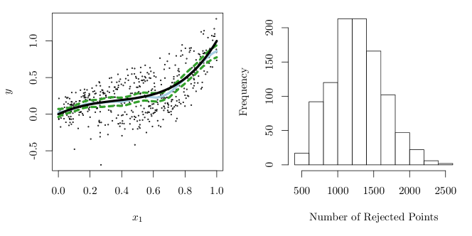
Figure 2: (Left) Plot of realized values of $X_{i1}$ against $Y_{i}$ for a single replication of the experiment, with solid black line indicating the true mean, light blue line indicating the estimated posterior mean, and the dashed green lines indicating 95% credible bands for the mean function. (Right) The posterior distribution of the number of rejected points estimated via Markov chain Monte Carlo.

Figure 2 displays a scatterplot of the relationship between $Y_{i}$ and $X_{i1}$ as well as the posterior mean and credible band for the function $r(x)=\mathbb{E}(Y_{i}\mid X_{i}=x)$ with $P=5$. We compare SBART-DS to a Dirichlet process mixture model described by Jara et al., (2011) as implemented in the function DPcdensity in the DPpackage package in R; we use this as a comparison because there is publicly available software implementing this methodology and Jara et al., (2011) show that it performs similarly to the approach of Dunson et al., (2007). This model uses the joint specification

$$(X_{i},Y_{i}) \sim\int\text{Normal}\left\{\begin{pmatrix}x\\ y\end{pmatrix}\mid\begin{pmatrix}\mu_{x}\\ \mu_{y}\end{pmatrix},\begin{pmatrix}\Sigma_{xx}&\Sigma_{xy}\\ \Sigma_{yx}&\Sigma_{yy}\end{pmatrix}\right\}\ dG(\mu,\Sigma),$$

where $G\sim\text{DP}(\alpha G_{0})$ is a Dirichlet process with a normal-inverse-Wishart base measure $G_{0}\equiv\text{Normal}(\mu\mid m,\kappa_{0}\Sigma)\ \text{IW}(\Sigma\mid\nu,\Psi)$. The conditional density of $[Y_{i}\mid X_{i}=x]$ can be estimated from an infinite mixture model as

$$f(y\mid x)=\sum_{k=1}^{\infty}\omega_{k}(x)\ \text{Normal}(y\mid\mu_{y\mid x},\Sigma_{y\mid x})$$

where $\omega_{k}(x)\propto\pi_{k}\textnormal{Normal}(x\mid\mu_{x},\Sigma_{xx})$, $\mu_{y\mid x}=\mu_{y}+\Sigma_{yx}\Sigma_{xx}^{-1}(x-\mu_{x})$, and $\Sigma_{y\mid x}=\Sigma_{yy}-\Sigma_{yx}\Sigma_{xx}^{-1}\Sigma_{xy}$. We use the same prior specification as Jara et al., (2011) but with a larger value of $\nu$ to accommodate the fact that $\nu>P-1$ is required.

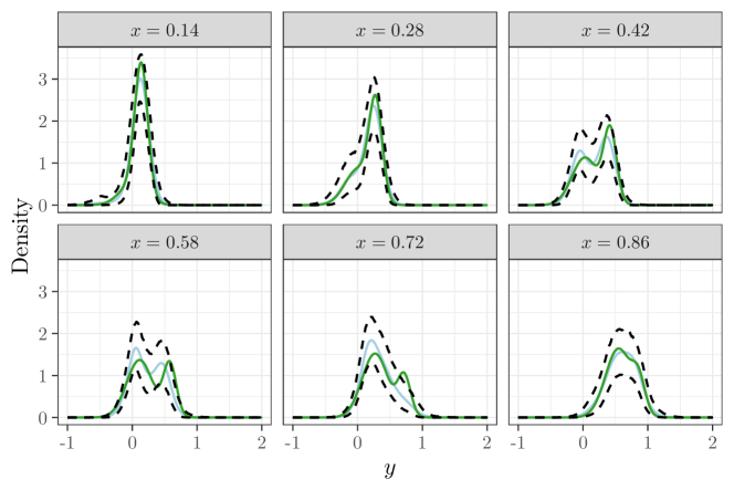
Figure 3: Posterior mean (blue), 95% credible bands for the density (dashed black) and true density function (green) for the simulated data, for the values $X_{i1}\in\{0.14,0.28,0.42,0.58,0.72,0.86\}$.

Figure 3 shows the fitted density for several fixed values of $X_{i1}$ with all other predictors frozen at the value $X_{ij}=0.5$ (as these predictors were correctly filtered out of the model, their particular value is irrelevant). We see SBART-DS successfully captures variability in the location, shape, and scale of the densities, and produces 95% credible bands which accurately account for uncertainty in the estimates. SBART-DS also captures the mean response accurately (left panel of Figure 2). Additionally, the number of rejected points is not prohibitively large, and fitting SBART-DS was faster than fitting the Dirichlet process mixture model using DPcdensity.

Table 1 compares SBART-DS to the Dirichlet process mixture over $100$ replications of the above experiment with $P=20$. We compare methods using the integrated total variation distance

$$\text{TV}(f_{0,}\widehat{f})=\int_{[0,1]^{P}}\int_{-\infty}^{\infty}|f_{0}(y\mid x)-\widehat{f}(y\mid x)|\ dy\ dx.$$

This integral can be approximated via Monte Carlo integration by averaging over a large out-of-sample test set of $X_{i}$’s and computing the $dy$ integral numerically. We see that the Dirichlet process mixture performs substantially worse than SBART-DS as measured by total variation distance from the true data generating mechanism. It is somewhat surprising that SBART-DS outperforms a Dirichlet process mixture for this example, as the true model is a mixture model with a structure that one would expect a Dirichlet process mixture to be primed to detect. The reason that SBART-DS performs better is that the BART prior we used performs variable selection and is capable of eliminating the $19$ irrelevant predictors, whereas the Dirichlet process mixture is not designed to detect sparsity. We expect that any method which does not explicitly try to detect sparsity, such as the probit stick-breaking prior with Gaussian processes proposed by Rodriguez and Dunson, (2011) or the kernel-based approach of Dunson et al., (2007) would also be outperformed by SBART-DS, although we were unable to assess this due to a lack of publicly available software for these approaches.

Method	Normalized Average $\text{TV}(f,\widehat{f})$	$25^{\text{th}}$ percentile	$75$ percentile
SBART-DS	1.00	0.94	1.05
Dirichlet Process Mixture	1.74	1.71	1.78

Table 1: Average of the integrated total variation distance $\text{TV}(f_{0},\widehat{f})$ over $100$ replications of the simulation study; to give a sense of stability, we also give the $25^{\text{th}}$ and $75^{\text{th}}$ quantiles of these quantities over the 100 replications. For interpretability, we normalized both scores by the average integrated total variation distance of the SBART-DS model.

Summarizing our simulation study, we find that the ability of SBART-DS to perform variable selection allows it to outperform Dirichlet process mixtures. While we only conducted a formal simulation study for the $P=20$ case, we found similar behavior for small values of $P$ as well. Unlike other Bayesian nonparametric density regression approaches, the ability to perform variable selection is automatic for SBART-DS.

5.2 Analysis of MEPS Data

We apply SBART-DS to data from the Medical Expenditure Panel Survey (MEPS) from the year 2015. MEPS is an ongoing survey in the United States which collects data on families/individuals, their medical providers, and employers, with a focus on the cost and use of health care.

There is a large literature which has considered the relationship between socioeconomic status, education, and obesity. Educational attainment relates to obesity in a complex fashion, with the effect modified by the overall income of a region, gender, and other factors (Cohen et al.,, 2013). We examined this relationship on a subset of the MEPS dataset consisting of responses from $1452$ women aged between $25$ and $35$ years old, controlling for log-income (measured as a percentage of the poverty line), age, and race. Existing research predicts that higher educational attainment will be associated with lower obesity levels in this group.

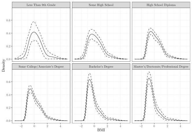
Figure 4: Density estimates and 95% credible bands for $f(y\mid x)$ for different educational levels for white women aged between 25 and 35, fixing log-income and age at their median values.

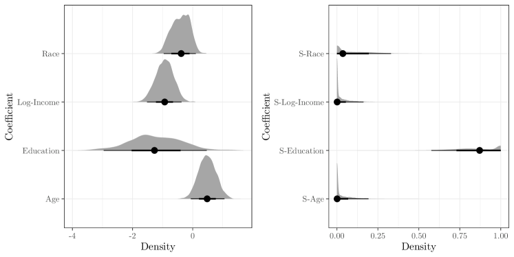
Figure 5: Left: Posterior medians, (66%, 95%)-credible intervals, and density estimates for the regression coefficients of the base mode $\beta_{\theta}$. Right: posterior medians, credible intervals, and density estimates for the splitting proportions $s_{j}$ for each predictor.

In Figure 4 we display the estimated density as the level of educational attainment is varied from less-than-high-school to graduate degree for white women with all other covariates frozen at their median value. We see that as educational attainment increases the bulk of the distribution remains concentrated near $0$ (the overall mean level of BMI) but goes from roughly symmetric to being highly right-skewed. The nature of this relationship is that, while the modal value BMI is fairly stable as education level changes, highly educated women are less likely to be highly obese.

Each predictor $j$ is associated to two coefficients: the base model coefficient $\beta_{\theta j}$ and the splitting proportion $s_{j}$. The posterior median, density, and a (66%, 95%)-credible interval is given for each coefficient in Figure 5. Interestingly, education level is the only relevant predictor in the selection model $\Phi\{r(y,x)\}$ so that the overall shape of the density is primarily determined by education. Intuitively, one might expect that education is only relevant through its indirect effect on income, however our results suggest this is not the case. Log-income has a strong presence in the base model as well, while race and age have weaker effects.

6 Discussion

In this paper we proposed a new method for density regression based on Bayesian additive regression trees. SBART-DS is suitable for routine use — it has a simple default specification, strong theoretical properties, and can be fit using a tuning-parameter-free Gibbs sampling algorithm. On simulated data we illustrated how SBART-DS is capable of filtering out irrelevant variables automatically, giving empirical support to the theoretical results supporting a faster posterior concentration rate when the rejection model $\Phi\{r(y,x)\}$ is sparse. Using data from MEPS we showed how SBART-DS can capture the effect of education level on the conditional distribution of body mass index.

The general strategy of defining a prior using a rejection sampling model can be used to extend that SBART-DS model to other domains. For example, this approach can be extended to survival analysis by modeling the hazard function $\lambda(y\mid x)$ as the hazard of a thinned Poisson process $\lambda(y\mid x)=\lambda_{0}(y\mid x)\ \Phi\{r(y,x)\}$. We will pursue this direction in future work.

Appendix A Proof of Auxiliary Results

Proof of Lemma 1.

For posterity, we note that Condition L implies $\frac{d}{d\mu}\log\Phi(\mu)\leq\mathcal{K}$; integrating both sides on an interval $[L,U]$ gives

$$e^{-\mathcal{K}(U-L)}\leq\frac{\Phi(L)}{\Phi(U)}\leq\frac{\Phi(U)}{\Phi(L)} \leq e^{\mathcal{K}(U-L)}.$$ (8)

Let $a=\sqrt{\Phi\{u(y,x)\}}$ and $b=\sqrt{\Phi\{v(y,x)\}}$ and let $\|a\|_{h}^{2}$ denote the squared $L_{2}$-norm $\int a^{2}(y,x)\ h(y)$ (which implicitly depends on $x$). Then

$$H(f_{u},f_{v})=\int\left\|\frac{a}{\|a\|_{h}}-\frac{b}{\|b\|_{h}}\right\|_{h}\ F_{X}(dx).$$

Two applications of the triangle inequality gives

$$H(f_{u},f_{v})\leq\int\frac{2\|a-b\|_{h}}{\|a\|_{h}}\ F_{X}(dx)\leq 2\|1-b/a\|_{\infty}.$$ (9)

The first inequality follows from the triangle inequality while the second follows from the inequality $\|a-b\|_{h}^{2}=\int a^{2}(y,x)\{1-b(y,x)/a(y,x)\}^{2}\ h(y)\leq\|a\|_{h}^{2}\cdot\|1-b/a\|_{\infty}^{2}$. Next, write $v(y,x)=u(y,x)+\Delta(y,x)$. Applying (8) and Taylor expanding the function $g(x)=\sqrt{\Phi(\mu+x)/\Phi(\mu)}$ we get

$$\left|1-\sqrt{\frac{\Phi\{v(y,x)\}}{\Phi\{u(y,x)\}}}\right| \leq|\Delta(y,x)|\frac{\phi\{u(y,x)+\Delta_{1}(y,x)\}}{2\Phi\{u(y,x)+\Delta_{1}(y,x)\}}\ \sqrt{\frac{\Phi\{u(y,x)+\Delta_{1}(y,x)\}}{\Phi\{u(y,x)\}}}$$

$$\leq\frac{\mathcal{K}}{2}\|u-v\|_{\infty}\exp\left[\frac{\mathcal{K}\|u-v\|_{\infty}}{2}\right]$$

where $\Delta_{1}(y,x)$ is between $0$ and $\Delta(y,x)$. Combining this with (9), $H(f_{u},f_{v})\leq\mathcal{K}\|u-v\|_{\infty}\exp(\mathcal{K}\|u-v\|/2)$. By Lemma 8 of Ghosal and Van Der Vaart, (2007), we have

$$K(f_{u},f_{v}) \lesssim H^{2}(f_{u},f_{v})\left(1+\log\left\|\frac{f_{u}}{f_{v}}\right\|_{\infty}\right)\qquad\text{and}$$

$$V(f_{u},f_{v}) \lesssim H^{2}(f_{u},f_{v})\left(1+\log\left\|\frac{f_{u}}{f_{v}}\right\|_{\infty}\right)^{2}.$$

Using (8) we have

$$\frac{f_{u}(y\mid x)}{f_{v}(y\mid x)}=\frac{\Phi\{u(y,x)\}\int h(\widetilde{y})\ \frac{\Phi\{v(\widetilde{y},x)\}}{\Phi\{u(\widetilde{y},x)\}}\ \Phi\{u(\widetilde{y},x)\}\ d\widetilde{y}}{\Phi\{v(y,x)\}\int h(\widetilde{y})\ \Phi\{u(\widetilde{y},x)\}\ d\widetilde{y}}\leq\exp(2\mathcal{K}\|u-v\|_{\infty}).$$

Hence $\log\|f_{u}/f_{v}\|_{\infty}\leq 2\mathcal{K}\|u-v\|_{\infty}$. ∎

Proof of Proposition 3.

Consider an extended prior $\widetilde{\Pi}$ on the joint distribution of $(X_{i},Y_{i})$ which places a point mass at $F_{X}$. We now have that $f_{r}$ is contained in the integrated Hellinger and Kullback-Leibler neighborhoods whenever $(f_{r},F_{X})$ are in the usual Hellinger and Kullback-Leibler neighborhoods of $F_{0}(dx,dy)=f_{0}(y\mid x)\ dy\ F_{X}(dx)$, so that the problem reduces to the setting of iid random vectors. The conditions (a)—(c) match one-to-one with the conditions of the variant of Theorem 2.1 of Ghosal et al., (2000) used by Shen et al., (2013, page 627), and hence suffice to establish the desired rate of convergence. ∎

We now prove that Condition L holds for the logit and $t_{\nu}$ links.

Proposition 4.

If $\Phi(\mu)=e^{\mu}/(1+e^{\mu})$ then Condition L holds with $\mathcal{K}=1$. If $\Phi(\mu)=T_{\nu}(\mu)$ where $T_{\nu}$ is the distribution function of a $t_{\nu}$ random variable then Condition L holds with $\mathcal{K}=\sqrt{\nu}$. Conversely, suppose $Z$ is symmetric and has distribution function $\Phi(\mu)$ and $Z$ is light-tailed in the sense that for all $\mathcal{K}$ we have $\Pr(Z>z)<e^{-\mathcal{K}z}$ for sufficiently large $z$. Then Condition L fails for $\Phi(\mu)$. In particular, Condition L fails for the probit link.

Proof.

For the logistic link it is straight-forward to check that $\phi(\mu)/\Phi(\mu)=1-\Phi(\mu)\leq 1$. To prove the result for the $T_{\nu}$ link we begin by deriving a lower bound for the survival function $\bar{T}_{\nu}(\mu)=\int_{\mu}^{\infty}t_{\nu}(x)\ dx$ for $\mu>0$. Note that the density is $t_{\nu}(\mu)=c/(1+\mu^{2}/\nu)^{p}$ where $p=(\nu+1)/2$ and $c$ is a normalizing constant. Define $z_{0}=1+\mu^{2}/\nu$, $z=1+x^{2}/\nu$, $\theta_{0}=\arcsin(1/\sqrt{z_{0}})$ and $\theta=\arcsin(1/\sqrt{z})$. Then after routine substitutions we have

$$\bar{T}_{\nu}(\mu) =\int_{z_{0}}^{\infty}\frac{c\sqrt{\nu}}{2\sqrt{z-1}}z^{-p}\ dz=c\sqrt{\nu}\int_{0}^{\theta_{0}}\sin^{2p-2}(\theta)\ d\theta$$

$$\geq c\sqrt{\nu}\int_{0}^{\theta_{0}}\sin^{2p-2}(\theta)\ \cos(\theta)\ d\theta=\frac{c\sqrt{\nu}}{2p-1}z_{0}^{-p+1/2}.$$

Using this, the symmetry of the $t_{\nu}$ distribution, and substituting $2p-1=\nu$, we have

$$\frac{t_{\nu}(\mu)}{T_{\nu}(\mu)}\leq\frac{t_{\nu}(|\mu|)}{\bar{T}_{\nu}(|\mu|)}\leq\frac{c}{z_{0}^{p}}\cdot\frac{\sqrt{\nu}}{cz_{0}^{-p+1/2}}=\sqrt{\nu}z_{0}^{-1/2}\leq\sqrt{\nu}.$$

For the converse, set $U=0$ and $L=-z$ in (8) to get $\Pr(Z>z)\geq\Phi(0)e^{-\mathcal{K}z}$ for some $\mathcal{K}$. In particular, $\Pr(Z>z)\geq\exp(-2\mathcal{K}z)$ for large enough $z$. In the case of the probit link, no such $\mathcal{K}$ can exist because $\Pr(Z>z)\leq e^{-z^{2}/2}$. ∎

The proof of Theorem 1 also requires a tail probability bound for the number of trees in the ensemble.

Proposition 5.

Let $\Pi(M=t)$ satisfy Condition P1. Then there exist constants $C^{\prime}_{M1}$ and $C^{\prime}_{M2}$ such that $\Pi(M\geq t)\leq C^{\prime}_{M1}\exp\{-C^{\prime}_{M2}t\log t\}$.

Proof.

By the geometric series formula we have

$$\Pi(M\geq t)=C_{M1}\sum_{k=t}^{\infty}e^{-C_{M2}k\log k}\leq\frac{C_{M1}\exp\{-C_{M2}t\log t\}}{1-t^{-C_{M2}}}=\frac{C_{M1}\exp\{-C_{M2}(t-1)\log t\}}{t^{C_{M2}}-1}.$$

For $t>2\vee 2^{1/C_{M2}}$ this gives $\Pi(M\geq t)\leq C_{M1}\exp\{-(C_{M2}/2)t\log t\}$. The result follows by taking $C^{\prime}_{M2}=C_{M2}/2$ and $C^{\prime}_{M1}$ to be the maximum of $C_{M1}$ and $\exp\{(C_{M2}/2)t\log t\}$ for $t\leq 2\vee 2^{1/C_{M2}}$. ∎

Appendix B Proof of Theorem 1

For completeness, we state two results of Linero and Yang, (2018) which will be used in the proof. These two propositions capture the features of SBART that make it useful in high-dimensional sparse settings with smooth regression functions.

Proposition 6.

Suppose that Condition F and Condition P are satisfied and $t\geq\alpha(D+1)/(2\alpha+D)$. Then there exist constants $B$ and $C$ independent of $(n,P)$ such that for all sufficiently large $n$ the prior satisfies

$$\Pi(\|r-r_{0}\|\leq B\epsilon_{n})\geq e^{-C\epsilon_{n}^{2}},$$

where $\epsilon_{n}=n^{-\alpha/(2\alpha+D)}\log(n)^{t}+\sqrt{D\log(P+1)/n}$.

Proof.

This is implied by Theorem 2 of Linero and Yang, (2018); the only modification required is that Condition P1 and Condition P2 are modified from Linero and Yang, (2018), but these modifications do not change the proof strategy. ∎

Proposition 7.

For fixed positive constants $\epsilon,\sigma_{1},\sigma_{2},T,A$ and integers $n,H,d$ define the set

$$\mathcal{G}= \Big{\{}f(\cdot)=\sum_{t=1}^{T}g(\cdot;\mathcal{T}_{t},\mathcal{M}_{t}):\ T\leq An\epsilon^{2},\text{ each tree has depth at most }H,$$

$$\text{the common bandwidth parameter $\tau$ satisfies }\sigma_{1}\leq\tau^{-1}\leq\sigma_{2},$$

$$\text{the total number of splitting directions is at most }d\text{ out of $P+1$},$$

$$\text{for each $(t,\ell),$ }\mu_{t\ell}\in[-U,U]\Big{\}}.$$

Then there exists a constant $C_{\psi}$ depending only the gating function $\psi$ of the SBART prior satisfying Condition P such that the following holds:

1. Covering entropy control: $\log N(\mathcal{G},C_{\psi}\varepsilon,\|\cdot\|_{\infty})\leq d\log(P+1)+3An\varepsilon^{2}\,2^{H}\log\big{(}d\,\sigma_{1}^{-1}\sigma_{2}^{2}An\varepsilon\,2^{H}U\big{)}$; and

2. Complement probability bound: if $H\geq d_{0}$, then $\Pi(\mathcal{G}^{c})\leq C^{\prime}_{M1}\exp\{-C^{\prime}_{M2}\,An\varepsilon^{2}\log(An\epsilon^{2})\}+2^{H}\,An\varepsilon^{2}$ $\cdot\big{[}\exp\{-E\,d\log(P+1)\}+C_{\mu 1}\,\exp\{-U^{C_{\mu 2}}\}\big{]}+C_{\tau 1}\,\exp\{-\sigma_{1}^{-C_{\tau 2}}\}+C_{\tau 3}\exp\{-\sigma_{2}^{C_{\tau 4}}\}$ for some constant $E>0$ depending only on hyperparameter $\xi>1$ in the Dirichlet prior.

Proof.

The proof is the same as the proof of Lemma 1 of the supplementary material of Linero and Yang, (2018), except that Proposition 5 is used in the complementary probability bound. ∎

Proof of Theorem 1.

Let $B$ and $C$ be chosen as in Proposition 6. By Lemma 1, note that for sufficiently large $n$, we have $\{f_{r}:\|r-r_{0}\|\leq B\epsilon_{n}\}\subseteq K(BC_{\mathcal{K}}\epsilon_{n})$ and $\{f_{r}:\|r-r_{0}\|\leq\epsilon_{n}\}\subseteq\{f_{r}:H(f_{r},f_{r_{0}})\leq C_{\mathcal{K}}\epsilon_{n}\}$ where $C_{\mathcal{K}}$ is a constant depending only on $\mathcal{K}$. Hence

$$\Pi\{f\in K(BC_{\mathcal{K}}\epsilon_{n})\}\geq e^{-Cn\epsilon_{n}^{2}}.$$

To lighten notation, we redefine $\epsilon_{n}$ throughout the rest of the proof to be $\epsilon_{n}BC_{\mathcal{K}}$ and $C$ to be $C/(BC_{\mathcal{K}})^{2}$ so that we have $\Pi\{f\in K(\epsilon_{n})\}\geq e^{-Cn\epsilon_{n}^{2}}$. This verifies (c) of Proposition 3 using the modified choice of $\epsilon_{n}$.

Next, for a large constant $\kappa$ to be chosen later, set $A=\kappa/\log n$, $\sigma_{1}^{-C_{\tau 2}}=\sigma_{2}^{C_{\tau 4}}=U^{C_{\mu 2}}=\kappa n\epsilon_{n}^{2}$, $H=d_{0}$, and $d=\lfloor\kappa n\epsilon_{n}^{2}/\log(P+1)\rfloor$ for the set $\mathcal{G}_{n}$ in Proposition 7. Plugging these constants into the covering entropy bound, for sufficiently large $n$ this implies that for $p_{1}=2+C_{\mu 2}^{-1}+C_{\tau 2}^{-1}+2C_{\tau 4}^{-1}$ and $p_{2}=2p_{1}-1$ we have

$$\log N(\mathcal{G}_{n},C_{\psi}\epsilon_{n},\|\cdot\|_{\infty})\leq\kappa n\epsilon_{n}^{2}\left\{1+\frac{3\cdot 2^{d_{0}}}{\log n}\log\left(\frac{2^{d_{0}}(\kappa n)^{p_{1}}\epsilon_{n}^{p_{2}}}{\log n}\right)\right\}\leq\kappa^{\prime}n\epsilon_{n}^{2}$$

for some $\kappa^{\prime}$ larger than $\kappa$ depending only on $\kappa$ and the constants in Condition P. Define $\mathcal{F}_{n}=\{f_{r}:r\in\mathcal{G}_{n}\}$. By Lemma 1, for large enough $n$ any $C_{\psi}\epsilon_{n}$-net $\mathcal{G}_{\text{net}}$ for $\mathcal{G}_{n}$ can be converted into a $C_{\mathcal{K}}C_{\psi}\epsilon_{n}$-net $\mathcal{F}_{\text{net}}=\{f_{r}:r\in\mathcal{G}_{\text{net}}\}$ for $\mathcal{F}_{n}$. Hence we also have the bound

$$\log N(\mathcal{F}_{n},C_{\mathcal{K}}C_{\psi}\epsilon_{n},H)\leq\log N(\mathcal{G}_{n},C_{\psi}\epsilon_{n},\|\cdot\|_{\infty})\leq\kappa^{\prime}n\epsilon_{n}^{2}$$

which establishes condition (a) of Proposition 3 with $\bar{\epsilon}_{n}=C_{\mathcal{K}}C_{\psi}\epsilon_{n}$ and $C_{N}=\kappa^{\prime}/(C_{\mathcal{K}}C_{\psi})^{2}$. Finally, we show condition (b) holds. Applying the complementary probability bound we can make $\Pi(\mathcal{F}_{n}^{c})\leq\exp\{-(C+4)n\epsilon_{n}^{2}\}$ for any choice of $C$ by taking $\kappa$ sufficiently large. To see why, note for example that $n\epsilon_{n}^{2}\geq an^{b}$ for some positive constants $(a,b)$ so that for large $n$ we have

$$An\epsilon_{n}^{2}\log(An\epsilon_{n}^{2})\geq\kappa n\epsilon_{n}^{2}\left\{\frac{\log(\kappa/\log n)+\log a}{\log n}+b\right\}\geq\frac{\kappa b}{2}n\epsilon_{n}^{2}.$$

Using similar arguments, for large $n$ we can bound each term of the complementary probability bound by $\exp\{-\kappa\delta n\epsilon_{n}^{2}/2\}$ for some $\delta$ depending only on the constants in Condition P. Taking $\kappa$ sufficiently large we can make the total bound less than $\exp\{-(C+4)n\epsilon_{n}^{2}\}$ for arbitrary $C$. This proves condition (b). ∎

References

- Albert and Chib, (1993) Albert, J. H. and Chib, S. (1993). Bayesian analysis of binary and polychotomous response data. Journal of the American Statistical Association, 88(422):669–679.
- Bleich and Kapelner, (2014) Bleich, J. and Kapelner, A. (2014). Bayesian additive regression trees with parametric models of heteroskedasticity. arXiv preprint arXiv:1402.5397.
- Brookes, (2011) Brookes, M. (2011). The matrix reference manual. Online. Accessed December 2019 at http://www.ee.imperial.ac.uk/hp/staff/dmb/matrix/intro.html.
- Chipman et al., (1998) Chipman, H. A., George, E. I., and McCulloch, R. E. (1998). Bayesian CART model search. Journal of the American Statistical Association, 93(443):935–948.
- Chipman et al., (2010) Chipman, H. A., George, E. I., and McCulloch, R. E. (2010). BART: Bayesian additive regression trees. The Annals of Applied Statistics, 4(1):266–298.
- Cohen et al., (2013) Cohen, A. K., Rai, M., Rehkopf, D. H., and Abrams, B. (2013). Educational attainment and obesity: A systematic review. Obesity Reviews, 14:989–1005.
- Dunson and Park, (2008) Dunson, D. B. and Park, J.-H. (2008). Kernel stick-breaking processes. Biometrika, 95(2):307–323.
- Dunson et al., (2007) Dunson, D. B., Pillai, N., and Park, J. H. (2007). Bayesian density regression. Journal of the Royal Statistical Society, Series B, 69:163–183.
- Dunson and Xing, (2009) Dunson, D. B. and Xing, C. (2009). Nonparametric bayes modeling of multivariate categorical data. Journal of the American Statistical Association, 104(487):1042–1051.
- Dutordoir et al., (2018) Dutordoir, V., Salimbeni, H., Hensman, J., and Deisenroth, M. (2018). Gaussian process conditional density estimation. In Advances in Neural Information Processing Systems, pages 2385–2395.
- Ghosal et al., (2000) Ghosal, S., Ghosh, J. K., and van der Vaart, A. W. (2000). Convergence rates of posterior distributions. Annals of Statistics, 28(2):500–531.
- Ghosal and Van Der Vaart, (2007) Ghosal, S. and Van Der Vaart, A. (2007). Posterior convergence rates of Dirichlet mixtures at smooth densities. The Annals of Statistics, 35(2):697–723.
- Holmes and Held, (2006) Holmes, C. C. and Held, L. (2006). Bayesian auxiliary variable models for binary and multinomial regression. Bayesian analysis, 1(1):145–168.
- Irsoy et al., (2012) Irsoy, O., Yildiz, O. T., and Alpaydin, E. (2012). Soft decision trees. In Proceedings of the International Conference on Pattern Recognition.
- Jara et al., (2011) Jara, A., Hanson, T. E., Quintana, F. A., Müller, P., and Rosner, G. L. (2011). Dppackage: Bayesian semi- and nonparametric modeling in R. Journal of Statistical Software, 40:1–30.
- Kundu and Dunson, (2014) Kundu, S. and Dunson, D. B. (2014). Latent factor models for density estimation. Biometrika, 101(3):641–654.
- Linero, (2018) Linero, A. R. (2018). Bayesian regression trees for high-dimensional prediction and variable selection. Journal of the American Statistical Association, 113(522):626–636.
- Linero et al., (2018) Linero, A. R., Sinha, D., and Lipsitz, S. R. (2018). Semiparametric Mixed-Scale Models Using Shared Bayesian Forests. arXiv e-prints arXiv:1809.08521.
- Linero and Yang, (2018) Linero, A. R. and Yang, Y. (2018). Bayesian regression tree ensembles that adapt to smoothness and sparsity. Journal of the Royal Statistical Society: Series B (Statistical Methodology), 80(5):1087–1110.
- MacEachern, (1999) MacEachern, S. N. (1999). Dependent nonparametric processes. In ASA Proceedings of the Section on Bayesian Statistical Science, pages 50–55.
- Murray et al., (2009) Murray, I., MacKay, D., and Adams, R. P. (2009). The gaussian process density sampler. In Koller, D., Schuurmans, D., Bengio, Y., and Bottou, L., editors, Advances in Neural Information Processing Systems 21, pages 9–16. Curran Associates, Inc.
- Neal, (1995) Neal, R. M. (1995). Bayesian Learning For Neural Networks. PhD thesis, University of Toronto.
- Pati et al., (2013) Pati, D., Dunson, D. B., and Tokdar, S. T. (2013). Posterior consistency in conditional distribution estimation. Journal of Multivariate Analysis, 116:456–472.
- Pratola et al., (2017) Pratola, M., Chipman, H., George, E., and McCulloch, R. (2017). Heteroscedastic BART using multiplicative regression trees. arXiv preprint arXiv:1709.07542.
- Rahimi and Recht, (2008) Rahimi, A. and Recht, B. (2008). Random features for large-scale kernel machines. In Platt, J. C., Koller, D., Singer, Y., and Roweis, S. T., editors, Advances in Neural Information Processing Systems 20, pages 1177–1184. Curran Associates, Inc.
- Rao et al., (2016) Rao, V., Lin, L., and Dunson, D. B. (2016). Data augmentation for models based on rejection sampling. Biometrika, 103(2):319–335.
- Ravikumar et al., (2007) Ravikumar, P., Liu, H., Lafferty, J., and Wasserman, L. (2007). SPAM: Sparse additive models. In Proceedings of the 20th International Conference on Neural Information Processing Systems, pages 1201–1208.
- Rockova and van der Pas, (2017) Rockova, V. and van der Pas, S. (2017). Posterior concentration for Bayesian regression trees and their ensembles. arXiv preprint arXiv:1078.08734.
- Rodriguez and Dunson, (2011) Rodriguez, A. and Dunson, D. B. (2011). Nonparametric bayesian models through probit stick-breaking processes. Bayesian analysis (Online), 6(1).
- Shen et al., (2013) Shen, W., Tokdar, S. T., and Ghosal, S. (2013). Adaptive Bayesian multivariate density estimation with Dirichlet mixtures. Biometrika, 100(3):623–640.
- Starling et al., (2018) Starling, J. E., Murray, J. S., Carvalho, C. M., Bukowski, R. K., and Scott, J. G. (2018). BART with targeted smoothing: An analysis of patient-specific stillbirth risk. arXiv:1805.07656.
- Tokdar et al., (2010) Tokdar, S. T., Zhu, Y. M., Ghosh, J. K., et al. (2010). Bayesian density regression with logistic gaussian process and subspace projection. Bayesian analysis, 5(2):319–344.
- van der Vaart and van Zanten, (2008) van der Vaart, A. W. and van Zanten, J. H. (2008). Rates of contraction of posterior distributions based on gaussian process priors. The Annals of Statistics, pages 1435–1463.
- Wang and Neal, (2012) Wang, C. and Neal, R. M. (2012). Gaussian process regression with heteroscedastic or non-gaussian residuals. arXiv preprint arXiv:1212.6246.
- Yang and Tokdar, (2015) Yang, Y. and Tokdar, S. T. (2015). Minimax-optimal nonparametric regression in high dimensions. The Annals of Statistics, 43(2):652–674.