Uncovering the hierarchical structure of the international FOREX market by using similarity metric between the fluctuation distributions of currencies

Abstract

The decentralized international market of currency trading is a prototypical complex system having a highly heterogeneous composition. To understand the hierarchical structure relating the price movement of different currencies in the market, we have focused on quantifying the degree of similarity between the distributions of exchange rate fluctuations. For this purpose we use a metric constructed using the Jensen-Shannon divergence between the normalized logarithmic return distributions of the different currencies. This provides a novel method for revealing associations between currencies in terms of the statistical nature of their rate fluctuations, which is distinct from the conventional correlation-based methods. The resulting clusters are consistent with the nature of the underlying economies but also show striking divergences during periods of major international crises.

I Introduction

One of the biggest challenges facing physicists trying to understand natural and man-made complex systems is to uncover principles underlying their collective dynamics. Socio-economic phenomena, in particular, provide examples of systems that exhibit a high degree of heterogeneity in the dynamical behavior exhibited by their components Sinha2011 . Unlike the dynamical systems traditionally investigated by physicists, such as arrays of coupled oscillators, coupling between the different parts of such complex systems do not necessarily result in the components displaying similar behavior (analogous to synchronization in oscillator arrays Pikovsky2001 ). Instead, autonomous agents in economic systems may employ various strategies which could manifest in different segments of the system exhibiting qualitatively distinct behavior Menon2019 . This is observed, for instance, in a financial market whose collective dynamics can be described in terms of the price movements of the numerous assets that are traded in it. These movements are not independent of each other as the components of this complex system “interact” through the actions of agents (ranging from individual investors to large financial institutions) buying and selling these assets. The statistical properties of the asset price fluctuations can differ remarkably from one asset to another, which can be linked to intrinsic, as well as, extrinsic factors. To understand the mechanisms through which such properties emerge, we first need to describe accurately how the fluctuations of the different components are related to each other.

In this paper, we consider the largest financial market in the world, the international currency or foreign exchange (FOREX) market BIS2013 . To provide a comparison, the average daily turnover in the FOREX market was $5.3\times 10^{12}$ USD in April 2013 while the average daily turnover for New York Stock Exchange, the biggest stock market in the world, in 2013 was $1.69\times 10^{11}$ USD. It is a decentralized global market for trading currencies which plays a key role in the international monetary and financial system. Furthermore, it is among the freest and most competitive markets in the world. The foreign exchange market is particularly important to complex systems researchers because of the large volumes of data it is able to provide for statistical analysis.

Currency exchange rates fluctuate because of a number of reasons, including the balance of trade, interest rate, monetary policies, etc. As such it is very difficult to discern the individual role that these different factors play in influencing the price fluctuations of a currency. Instead, we propose to uncover the hierarchical structure of the network relating the different currencies in terms of their fluctuation behavior. We use a metric for measuring the distance between pairs of exchange rate fluctuation distributions to cluster the currencies (and by extension, the economies to which they belong) into similarity groups. This provides a novel approach to grouping components in complex systems according to the statistical characteristics of their dynamical behavior, distinct from the widely employed method of using cross-correlations between the time-series Laloux1999 ; Plerou1999a ; McDonald2005 ; Pan2007 ; Kovur2014 which have limitations Reshef2011 ; Kinney2014 . We have also performed a temporally resolved analysis of the nature of the distributions at different periods that shows strong disruption in the otherwise regular pattern of systematic variations during the global financial crisis of 2008, indicating its deep-rooted nature affecting the real economy Claessens2012 ; Kenourgios2015 .

Table 1: The currencies of developed (1-14), emerging (15-44) and frontier (45-75) economies considered in the study. The columns indicate the currency code along with the nature of the exchange rate regime (as obtained from Oanda and XE sites), the character of the economy (as categorized by MSCI) and the geographical region of the corresponding countries.

Sl. no.	Currency	Code	Exchange Rate Regime	Market Type	Region
			(Oanda, XE)	(MSCI)
1	Canadian Dollar	CAD	Floating	Developed	Americas
2	Danish Krone	DKK	Pegged within horizontal band	Developed	Europe
3	Euro	EUR	Floating	Developed	Europe
4	Great Britain Pound	GBP	Floating	Developed	Europe
5	Iceland Krona	ISK	Floating	Developed	Europe
6	Norwegian Kroner	NOK	Floating	Developed	Europe
7	Swedish Krona	SEK	Floating	Developed	Europe
8	Swiss Franc	CHF	Floating	Developed	Europe
9	Israeli New Shekel	ILS	Floating	Developed	Middle East
10	Australian Dollar	AUD	Floating	Developed	Asia-Pacific
11	Hong Kong Dollar	HKD	Fixed peg	Developed	Asia-Pacific
12	Japanese Yen	JPY	Floating	Developed	Asia-Pacific
13	New Zealand Dollar	NZD	Floating	Developed	Asia-Pacific
14	Singapore Dollar	SGD	Floating	Developed	Asia-Pacific
15	Bolivian Boliviano	BOB	Crawling peg	Emerging	Americas
16	Brazilian Real	BRL	Floating	Emerging	Americas
17	Chilean Peso	CLP	Floating	Emerging	Americas
18	Colombian Peso	COP	Floating	Emerging	Americas
19	Dominican Republic Peso	DOP	Floating	Emerging	Americas
20	Mexican Peso	MXN	Floating	Emerging	Americas
21	Peruvian Nuevo Sol	PEN	Floating	Emerging	Americas
22	Venezuelan Bolivar	VEB	Fixed peg	Emerging	Americas
23	Albanian Lek	ALL	Floating	Emerging	Europe
24	Czech Koruna	CZK	Floating	Emerging	Europe
25	Hungarian Forint	HUF	Pegged within horizontal band	Emerging	Europe
26	Polish Zloty	PLN	Floating	Emerging	Europe
27	Russian Rouble	RUB	Floating	Emerging	Europe
28	Turkish Lira	TRY	Floating	Emerging	Europe
29	Algerian Dinar	DZD	Floating	Emerging	Africa
30	Cape Verde Escudo	CVE	Fixed peg	Emerging	Africa
31	Egyptian Pound	EGP	Floating	Emerging	Africa
32	Ethiopian Birr	ETB	Floating	Emerging	Africa
33	Mauritius Rupee	MUR	Floating	Emerging	Africa
34	Moroccan Dirham	MAD	Fixed peg	Emerging	Africa
35	South African Rand	ZAR	Floating	Emerging	Africa
36	Tanzanian Shilling	TZS	Floating	Emerging	Africa
37	Chinese Yuan Renminbi	CNY	Fixed peg	Emerging	Asia
38	Indian Rupee	INR	Floating	Emerging	Asia
39	Indonesian Rupiah	IDR	Floating	Emerging	Asia
40	Papua New Guinea Kina	PGK	Floating	Emerging	Asia
41	Philippine Peso	PHP	Floating	Emerging	Asia
42	South Korean Won	KRW	Floating	Emerging	Asia
43	Taiwan Dollar	TWD	Floating	Emerging	Asia
44	Thai Baht	THB	Floating	Emerging	Asia
45	Guatemalan Quetzal	GTQ	Floating	Frontier	Americas
46	Honduran Lempira	HNL	Crawling peg	Frontier	Americas
47	Jamaican Dollar	JMD	Floating	Frontier	Americas
48	Paraguay Guarani	PYG	Floating	Frontier	Americas
49	Trinidad Tobago Dollar	TTD	Floating	Frontier	Americas
50	Croatian Kuna	HRK	Floating	Frontier	Europe
51	Kazakhstan Tenge	KZT	Floating	Frontier	Europe
52	Latvian Lats	LVL	Fixed peg	Frontier	Europe
53	Botswana Pula	BWP	Crawling peg	Frontier	Africa
54	Comoros Franc	KMF	Fixed peg	Frontier	Africa
55	Gambian Dalasi	GMD	Floating	Frontier	Africa
56	Ghanaian Cedi	GHC	Floating	Frontier	Africa
57	Guinea Franc	GNF	Fixed peg	Frontier	Africa
58	Kenyan Shilling	KES	Floating	Frontier	Africa
59	Malawi Kwacha	MWK	Floating	Frontier	Africa
60	Mauritanian Ouguiya	MRO	Floating	Frontier	Africa
61	Mozambique Metical	MZM	Floating	Frontier	Africa
62	Nigerian Naira	NGN	Floating	Frontier	Africa
63	Sao Tome and Principe Dobra	STD	Fixed peg	Frontier	Africa
64	Zambian Kwacha	ZMK	Floating	Frontier	Africa
65	Jordanian Dinar	JOD	Fixed peg	Frontier	Middle East
66	Kuwaiti Dinar	KWD	Fixed peg	Frontier	Middle East
67	Syrian Pound	SYP	Fixed peg	Frontier	Middle East
68	Brunei Dollar	BND	Fixed peg	Frontier	Asia
69	Bangladeshi Taka	BDT	Floating	Frontier	Asia
70	Cambodian Riel	KHR	Floating	Frontier	Asia
71	Fiji Dollar	FJD	Fixed peg	Frontier	Asia
72	Lao Kip	LAK	Floating	Frontier	Asia
73	Pakistan Rupee	PKR	Floating	Frontier	Asia
74	Samoan Tala	WST	Fixed peg	Frontier	Asia
75	Sri Lankan Rupee	LKR	Floating	Frontier	Asia

II Materials and Methods

In this study we have analyzed a data-set comprising the daily exchange rates of $N=75$ currencies (see Table 1) with respect to the US Dollar (USD), for the period October 23, 1995 to February 10, 2016, corresponding to $\tau=7416$ days. Specifically, we use the midpoint between the bid and ask rates for 1 USD against a given currency. The source of the data is an online archive of historical interbank market rates made available by the Oanda Corporation Oanda which provides internet-based currency trading and information services. The interbank rate (also referred to as spot rate) is used for large volume transactions carried out by banks and financial institutions, and is the exchange rate that is typically reported in the media. From the online archive we have obtained the rate for each day in the period under consideration, averaged over all quotations collected within the previous 24 hour period (terminating at midnight UTC) from various frequently updated sources around the world, including online currency trading platforms, market data vendors, and contributing financial institutions. The USD is chosen as the numeraire as it is the preferred currency for most international transactions and continues to remains the reserve currency of choice for many economies Papaioannou2006 ; IMFAnnRep .

To see how the use of a particular numeraire, viz., the USD, may have introduced bias in the results reported here, we have also carried out our analysis by expressing the exchange rates of currencies in terms of Special Drawing Rights (SDR), a supplementary international reserve asset created by the International Monetary Fund (IMF), whose value is determined by a basket of currencies SDR . The composition of the basket is altered regularly to ensure that it reflects the relative importance of different currencies in international trade and finance. Daily quotes for SDR in terms of USD is available from the IMF IMFdata for all days (except those on which IMF is closed for business, which include weekends). We have used this to create a daily exchange rate time-series with SDR as the numeraire, spanning the $5210$ days for which data is available in the period under study.

The $75$ currencies considered in our study are chosen based on the exchange rate regime followed by them (see Table 1). The information about the regime type of each currency has been obtained from the same online source from which we have collected the daily rates Oanda , supplemented with information from the website of another online foreign exchange tools and services company xe . We have explicitly avoided any currency whose exchange rate with respect to USD does not vary over time. Most of the currencies chosen for our analysis are either freely floating under the influence of market forces or managed to an extent with no pre-determined path. The remainder, although pegged to USD or some other important currency (such as EUR), do exhibit variation within a band which may be either fixed or can change over time. We have also classified the economy of the countries to which these currencies belong by using the Morgan Stanley Capital International (MSCI) market classification framework MSCI . Using multiple criteria including the sustainability of economic development, the number of companies meeting certain size and liquidity criteria, ease of capital flow, as well as, efficiency and stability of the institutional framework, MSCI classifies the economies into three categories, viz., developed, emerging and frontier markets (see Table 1). An important point to note is that for the period prior to January 1, 1999, when the EUR was first introduced, we have used in its stead the exchange rate for the ECU (European Currency Unit).

III Results

Instead of analyzing the raw price information, the fluctuations in the exchange rates of 75 currencies (see Table 1) with respect to the US Dollar over the period 1995-2016 is measured. To make the result independent of the unit of measurement, the variation in the exchange rate $P_{i}(t)$ of the $i$-th currency ($i=1,\ldots,N$) at time $t$ is quantified by its logarithmic return defined over a time-interval $\Delta t$ as $R_{i}(t,\Delta t)=ln\,P_{i}(t+\Delta t)-ln\,P_{i}(t)$. Since our data comprises the daily exchange rates, we consider $\Delta t=1$ day. The standard deviation $\sigma$ of the returns measures the intensity of fluctuations in the exchange rates (volatility) which varies for different currencies. Hence, to compare between the return distributions of different currencies, we normalize the returns of each currency $i$ by subtracting the mean value $\langle R_{i}\rangle=\Sigma_{t=1}^{T}R_{i}(t)/T$ and dividing by the standard deviation $\sigma_{i}(t)=\sqrt{\frac{1}{T-2}\Sigma_{t^{\prime}\neq t}[R_{i}(t^{\prime})-\langle R_{i}\rangle]^{2}}$ (removing the self contribution from the measure of volatility), obtaining the normalized return, $r_{i}(t)=(R_{i}(t)-\langle R_{i}\rangle)/\sigma_{i}(t)$.

III.1 Hierarchical clustering based on similarity of fluctuations distribution

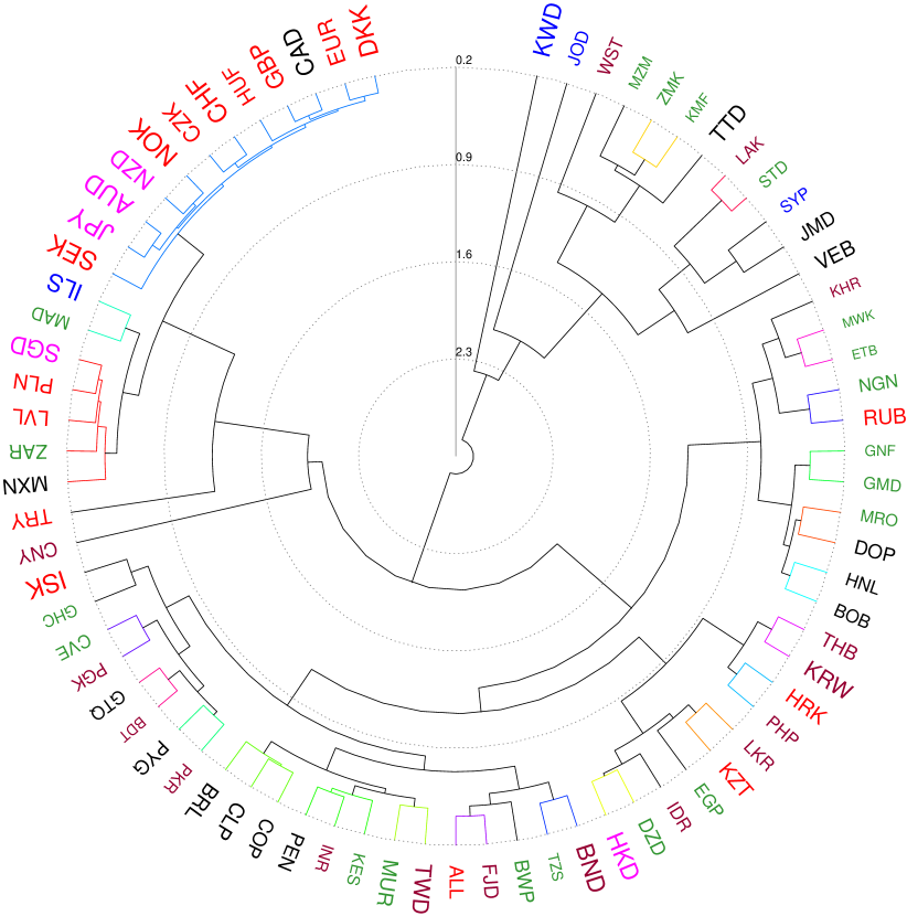
Figure 1: Polar dendrogram representation obtained by hierarchical clustering of different currencies in terms of the statistical distance between their fluctuation distributions. A similarity distance $D$ obtained from the Jensen-Shannon divergence between the corresponding normalized logarithmic return distributions of a pair of currencies has been used as the clustering metric. The currencies have been clustered using complete linkage algorithm and the height of a branch measures the linkage function $d$, i.e., the distance between two clusters. Using a threshold of $d_{th}=0.47$, the largest number of distinct clusters (viz., 22 clusters represented by the different colored branches of the dendrogram, black branches indicating isolated nodes) can be identified. The largest cluster comprises only currencies of developed economies with the exception of CZK and HUF (belonging to emerging economies). Currencies are distinguished according to the average annual GDP per capita $\langle g\rangle$ of the corresponding economy (represented by font size, which scales logarithmically with $\langle g\rangle$) and the geographical region to which they belong (represented by font color, viz., black: Americas, red: Europe, blue: Middle East, magenta: Asia-Pacific, green: Africa and brown: Asia).

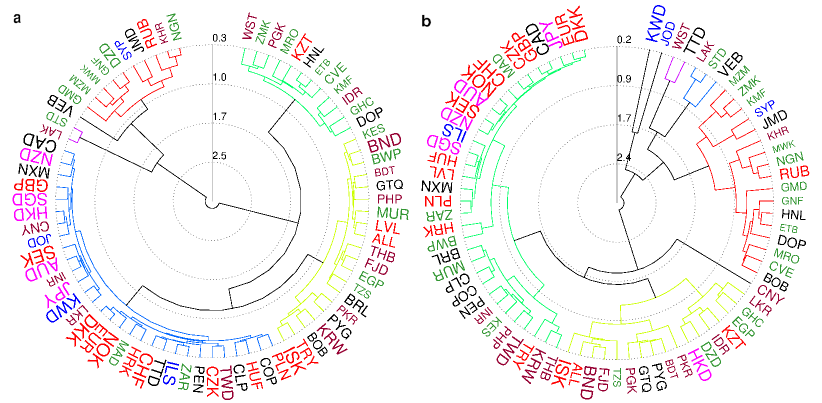
Figure 2: Comparison between hierarchical clustering of currencies according to the statistical distance between corresponding fluctuation distributions when the exchange rates are expressed in terms of different numeraires, viz., (a) SDR and (b) USD. As in Fig. 1, clustering is performed using complete linkage algorithm. In (a), using a threshold of $d_{th}=0.78$, $5$ distinct clusters, represented by the different colored branches of the dendrogram (with black branches indicating isolated nodes), can be identified. Note that the SDR data used for constructing the dendrogram is available only for $5210$ days during the period October 23, 1995 to February 10, 2016. Using this same set of dates, we have constructed in (b) a dendrogram from the data in which currency exchange rates are expressed in terms of USD, for comparison with (a). For a threshold of $d_{th}=1.30$, we observe $5$ distinct clusters in this case also. The cophenetic distance correlation coefficient between the two dendrograms is $0.52$, suggesting a high degree of similarity between them.

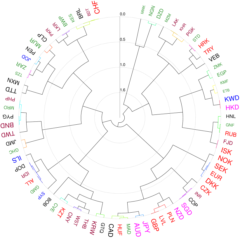
Figure 3: Polar dendrogram representation obtained by hierarchical clustering of different currencies on the basis of how similar they are in exhibiting extreme values in their exchange rates, i.e., in terms of the heavy-tailed nature of the fluctuation distributions. The relative difference between the kurtosis of corresponding normalized logarithmic return distributions of a pair of currencies has been used as the clustering metric. As in Fig. 1, clustering is performed using complete linkage algorithm. Using a threshold of $d_{th}=0.08$, the largest number of distinct clusters (viz., 24, represented by the different colored branches of the dendrogram, with black branches indicating isolated nodes) can be identified. Unlike the clusters obtained using Jensen-Shannon divergence shown in Fig. 1, all clusters here are relatively small. The relative dissimilarity between the clusters seen here and that in Fig. 1 is quantitatively indicated by the value of the cophenetic distance correlation coefficient between the two dendrograms being $0.2$. However, most of the currencies belonging to developed economies do seem to occur close to each other, with the exceptions of CHF, HKD and ISK (resulting from rare instances of extremely large deviations in their exchange rates). As in Fig. 1, currencies are distinguished according to the average annual GDP per capita $\langle g\rangle$ of the corresponding economy (represented by font size, which scales logarithmically with $\langle g\rangle$) and the geographical region to which they belong (represented by font color, viz., black: Americas, red: Europe, blue: Middle East, magenta: Asia-Pacific, green: Africa and brown: Asia).

We have investigated the inter-relation between the different currencies by considering how similar they are in terms of the nature of their fluctuations. For this we have measured the difference between the normalized logarithmic return distributions of each pair of currencies using a probability distance metric, viz., the similarity distance $D(P_{i},P_{j})$ between a pair of return distributions $P_{i}(r)$ and $P_{j}(r)$ Endres2003 . It is defined as the square root of the Jensen-Shannon (JS) divergence Lin1991 , which in turn can be defined in terms of the Kullback-Leibler (KL) divergence for a pair of probability distributions $P_{i}(x)$ and $P_{j}(x)$ of a discrete random variable $x$:

$$KL(P_{i},P_{j})=\sum_{x\in X}P_{i}(x)log\frac{P_{i}(x)}{P_{j}(x)}.$$

The limitations of the KL divergence, viz., that it is asymmetric and is, moreover, undefined when either $P_{i}$ or $P_{j}$ is zero for any value of $x\in X$, is overcome by the JS divergence which is defined as:

$$JS(P_{i},P_{j})=\frac{1}{2}KL(P_{i},P)+\frac{1}{2}KL(P_{j},P),$$

where, $P=(P_{i}+P_{j})/2$. As returns are continuous variables, in order to calculate the divergences between their distributions we have discretized the values using a binning procedure (involving intervals of width $\Delta r\sim 0.05$). The same binning procedure has been also used for the analysis described later in which the data is split into four non-overlapping segments belonging to different time periods. Note that, the related generalized JS measure has been used earlier to measure the similarity of tick frequency spectrograms for different currency exchange rates Sato .

The matrix of similarity distances $\cal D$ between all pair of currencies is used for clustering them in a hierarchical manner. Note that this approach is distinct from earlier attempts of hierarchical classification which use synchronous cross-correlation between exchange rate fluctuations in order to identify clusters of related currencies (see, e.g., Refs. Mizuno2006 ; Kwapien2009 ; Keskin2011 ). Given a set of nodes to be clustered and a matrix specifying the distances between them, the method of hierarchical clustering Johnson1967 involves (i) initially considering each node as a cluster, (ii) merging the pair of clusters which have the shortest distance between them, (iii) re-computing the distance between all clusters, and repeating the steps (ii) and (iii) until all nodes are merged into a single cluster. Clustering methods can differ in the way the inter-cluster distance is calculated in step (iii). If this distance is taken as the maximum of the pairwise distances between members of one cluster to members of the other cluster, it is known as complete-linkage clustering. On the other hand, in the single-linkage or nearest neighbor clustering, the minimum of the distance between any member of one cluster to any member of the other cluster is chosen. Average-linkage clustering, as the name implies, considers the mean of the pairwise distances between members of the two clusters. Note that, the hierarchical clustering obtained using the complete-linkage method will be same as one obtained using a threshold distance to define membership of a cluster, while that constructed using the single-linkage method is identical to the minimal spanning tree Gower1969 .

We have shown the hierarchical clustering (using complete-linkage clustering) of the different currencies considered in this study in Fig. 1 using a polar dendrogram representation. We note that the technique divides the currencies at the coarsest scale into two groups, the smaller of which is almost exclusively composed of currencies from frontier economies (the sole exception being VEB which belongs to an emerging economy) that are characterized by large fluctuations. Although some of these currencies (e.g., KWD, TTD and VEB) belong to countries having high GDP per capita, they typically also have a high Theil index Theil1967 indicating that their foreign trade is dominated by the export of a few key products (e.g., crude oil in the case of Kuwait, Trinidad & Tobago and Venezuela). Their currencies are therefore potentially highly susceptible to fluctuations in the worldwide demand. Focusing now on the larger group, we observe that it is further divided broadly into two subgroups, one of which is dominated by relatively stable currencies from developed and emerging economies, with only a single frontier economy being represented (viz., LVL) which has a relatively higher GDP per capita than the other frontier economies. The other subgroup is composed of currencies from emerging as well as frontier economies (with the exception of HKD and ISK which belong to developed economies). The occurrence of these latter two in this subgroup can be related to the severe financial crises encountered by these economies at different times, viz., the 2003 SARS crisis in the case of Hong Kong and the 2008 banking collapse in the case of Iceland, during the period under consideration. The largest number of similarity clusters into which the currencies can be grouped is obtained for a threshold value of $d_{th}=0.47$. Most of the currencies belonging to developed economies are seen to occur in the largest cluster consisting of 12 currencies, indicating that these economies have a relatively similar high degree of stability for their currency exchange rates. As expected, almost all of them have high GDP per capita. The only members of this highly stable currency cluster which are not in the developed category (viz., CZK and HUF) belong to countries that are members of the European Union, and whose economies are therefore highly integrated with the other members of this cluster. The second largest cluster comprising $5$ currencies also appear to bring together economies that have similar GDP per capita even though they vary in their market classification from developed (SGD) to emerging (MXN, PLN and ZAR) and frontier (LVL). The remaining clusters are mostly pairs (or at most triplets) of currencies.

To ensure that the hierarchical organization evident from the dendrogram is not too sensitively dependent on the specific numeraire we have used, in Fig. 2 we have compared dendrograms constructed using exchange rates expressed in terms of SDR and USD. As the daily quotes for SDR is available only for a subset of the dates for which we have information about the rates expressed in USD, for a fair comparison we have constructed the two dendrograms using the set of dates common between the two classes of data. As is evident, the clusters of currencies observed in the two hierarchical structures are qualitatively similar. The resemblance between the two dendrograms can be quantified by using the cophenetic distance correlation coefficient (CDCC). This is computed by measuring the cophenetic distance between pairs of elements, which is defined as the height of the branch where two elements become members of the same cluster in the dendrogram, and then obtaining the correlation between the corresponding distances in the two dendrograms Sokal1962 ; Rohlf1981 ; Saracli2013 . The value of CDCC between the dendrograms shown in panels (a) and (b) of Fig. 2 is found to be 0.52, suggesting a high degree of similarity between them.

As the shape of a distribution can be described by its moments Gavriliadis2009 , to delve deeper into whether any specific property of the fluctuation distribution is responsible for the hierarchical clustering reported above, we have investigated the relation between the lowest order moments of the distributions for the different currencies. As we consider normalized returns, the first and second moments (corresponding to mean and variance) of all the distributions are identical. Furthermore, as most of the return distributions are approximately symmetric (large deviations being shown only by NGN, DZD, MWK, PGK, VEB, MZM, TRY, FJD and STD), the distributions do not also markedly differ in terms of their skewness (related to the third moment). Thus, we focus on the kurtosis, measured in terms of the fourth moment, which quantifies the probability of occurrence of extreme values reflected in the heavy-tailed nature of the distribution. Considering higher order moments is not likely to provide any further information as it is known that specifying a finite number of moments of a distribution only determines its tail but not its bulk Lindsay2000 .

For each pair of currencies $i,j$, we have measured the relative difference between the kurtosis $\alpha_{4}$ of their fluctuation distributions as

$$\delta(\alpha_{4}^{i},\alpha_{4}^{j})=\frac{|\alpha_{4}^{i}-\alpha_{4}^{j}|}{\langle\alpha_{4}^{i},\alpha_{4}^{j}\rangle},$$

where $\langle\ldots\rangle$ represents the mean. The matrix of these differences is then used to hierarchically cluster the currencies using the complete-linkage method. Fig. 3 shows the results of the clustering using a polar dendrogram representation. There are clearly discernible differences with the structure shown in Fig. 1, indicating that there are aspects of the distribution other than kurtosis (and hence, the behavior at the tails) which are responsible for the similarity in the nature of fluctuations of the currencies belonging to a cluster. The differences can partly be ascribed to the fact that the kurtosis is strongly affected by rare (or even single instances of) extreme events. For example, this is possibly the explanation for the adjacency of currencies DZD, NGN and MWK seen in Fig. 3, as all three experienced a large deviation in their exchange rates on November 7, 1995. This has been explicitly verified by reconstructing the dendrogram after discarding this specific extreme return value and noting that the three currencies no longer occur in close proximity. We also note that this single extreme event strongly affects the synchronous cross-correlations between the currency movements over the entire period under study, resulting in the three currencies being identified as a prominent cluster moving independently of other currencies Kovur2014 . This is apparent from the dendrogram shown in Fig. 4 which represents relations between the currencies in terms of the degree of synchrony in their fluctuations. It underlines one of the weaknesses of using cross-correlations between asset price fluctuations for inferring significant dynamical relationships between the assets, as a lone outlier may be sufficient to significantly bias the results obtained.

Another example of a rare event influencing the kurtosis is the occurrence of CHF (belonging to a developed economy) far from the neighborhood of the other currencies of developed economies. This can be traced to a rapid rise in its exchange rate immediately following the depegging of CHF from EUR in January 2015. If the clustering is performed by considering only the time period preceding this event, we note that CHF occurs along with the other currencies belonging to economies having similar character. We do note, however, that, in general, currencies belonging to similar economies tend to be grouped in neighboring locations in the dendrogram, which could be related to the fact that the kurtosis of the fluctuation distribution of a currency is related to the overall prosperity, as measured by the gross domestic product per capita, of the corresponding economy Chakraborty2018 .

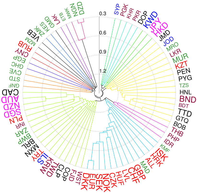
Figure 4: Polar dendrogram representation of the hierarchical clustering of currencies using synchronous cross-correlations between the time-series of their exchange rate fluctuations. Distance between each pair of currencies $i,j$ is computed from the Pearson correlation $C_{ij}$ between their normalized returns over the period under study as $d_{ij}=\sqrt{2(1-C_{ij})}$, following Ref. Mantegna1999 . As in Fig. 1, clustering is performed using complete linkage algorithm. For a threshold of $d_{th}=1.4$, $13$ distinct clusters represented by the different colored branches of the dendrogram (with black branches indicating isolated nodes) can be identified. Note the cluster of three currencies (comprising DZD, NGN and MWK) at the top. Their apparently strong association arises from a single extreme fluctuation event that occurred on November 7, 1995.

III.2 Temporal evolution of the system properties

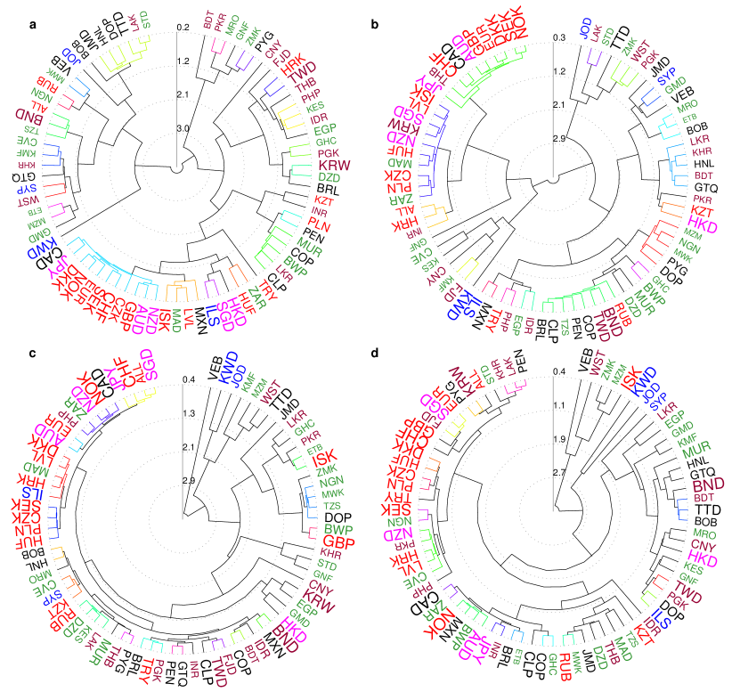
Figure 5: Temporal evolution of the hierarchical clustering of different currencies according to the similarity of their exchange rate fluctuation distributions. Dendrogram representations of the clusters constructed following the same procedure as for Fig. 1 are shown for four different time intervals: (a) Period I: Oct 23, 1995-Nov 18, 2000, (b) Period II: Nov 19, 2000- Dec 16, 2005, (c) Period III: Dec 17, 2005-Jan 13, 2011, and (d) Period IV: Jan 14, 2011-Feb 10, 2016. The threshold distances used for obtaining the largest number of clusters in each period are $d_{th}=0.80$, $0.90$, $0.70$ and $0.65$, which yield $19$, $16$, $17$ and $16$ clusters, respectively. Note that the statistical distance between the currencies shrink in the latter two periods following the major economic crisis that occurred in 2008. The cluster of currencies belonging to developed economies seen in the earlier periods is also seen to be disrupted to an extent. The degree of similarity between the different dendrograms is quantified by the cophenetic distance correlation coefficient as follows: CDCC(I,II) = $0.23$, CDCC(II,III)=$0.12$ and CDCC(III,IV)=$0.46$. As in Fig. 1, currencies are distinguished according to the average annual GDP per capita $\langle g\rangle$ of the corresponding economy (represented by font size, which scales logarithmically with $\langle g\rangle$) and the geographical region to which they belong (represented by font color, viz., black: Americas, red: Europe, blue: Middle East, magenta: Asia-Pacific, green: Africa and brown: Asia).

In the analysis presented above we have considered the entire temporal duration which our data-set spans. However, as the world economy underwent significant changes during this period, most notably, the global financial crisis of 2008, it is of interest to see how the hierarchical structure of the currency market has evolved over time. For this purpose we divide the data-set into four equal non-overlapping periods comprising 1853 days, corresponding to Period I: Oct 23, 1995 - Nov 18, 2000, Period II: Nov 19, 2000 - Dec 16, 2005, Period III: Dec 17, 2005 - Jan 13, 2011 and Period IV: Jan 14, 2011 - Feb 10, 2016. Note that Period III corresponds to the crisis of the global economy spanning 2007-2009 that also affected the FOREX market Melvin2009 , allowing us to contrast the structure of the currency market in the pre-crisis era (Periods I and II) with the situation that prevailed during the crisis, as well as, post-crisis (Period IV). For each of these periods, we carry out the same procedures as outlined earlier for the entire data-set.

The hierarchical clustering of the currencies show striking changes over time when they are constructed separately for each of the four intervals mentioned above (Fig. 5). The degree of similarity between the clusters seen in the four periods can be quantitatively indicated by the cophenetic distance correlation coefficient calculated for pairs of successive periods.The corresponding values, viz., CDCC(I,II) = $0.23$, CDCC(II,III)=$0.12$ and CDCC(III,IV)=$0.46$, suggest that a major disruption took place in the hierarchical structure in the period immediately leading upto the crisis.

As seen for the data-set covering the entire period, the method classifies the currencies in the pre-crisis era broadly into two groups with one group comprising the relatively stable currencies of developed and emerging economies. However, during and following the crisis, the broad division separates only a small group of frontier economy currencies (with the exception of VEB in Periods III and IV, and ISK in Period IV) from the rest. While the developed economies largely remain members of the same group even after the crisis, the relative position of most currencies show large changes. Even among the developed economy currencies, we observe that ISK moves away from its peers following the crisis. This is possibly related to the Icelandic crisis of 2008-2010 that saw a complete collapse of its financial system Carey2009 ; Sigurjonsson2011 . The severity of the global crisis of 2008 is also reflected in the movement of GBP away from the neighborhood of currencies belonging to the other developed economies in Period III, although it subsequently returned in Period IV to the group in which it belonged.

IV Discussion and Conclusion

In this work, we have used the Jensen-Shannon divergence, that measures the difference between two distributions, in a novel method for clustering currencies into similarity groups based on the statistical behavior of their fluctuations. In principle, one can use other definitions for the distance between probability distributions, such as the total variation distance and the Bhattacharyya distance Bhattacharyya1943 . In the case of the international currency market this approach is particularly apt, compared to correlation-based methods, for reconstructing the hierarchical network relating the movements of different currencies. This is because trading in different currencies is distributed across the globe, with activity in different locations (focused around specific sets of currencies) peaking at different times because of the corresponding time-zones. This is quite distinct from the situation for a stock market located in a specific geographical location, where trading in all assets begins and ends at the same time, which allows one to compute the synchronous correlations between the movements of the different assets. In contrast, when information about trading in different currencies is pooled together over a given 24 hour period, one may be comparing the movement of a particular currency at the beginning of the trading day in the location where trading in it is most intense with that of another currency at the close of the trading day in a different location which focuses on trading in the latter. This makes it essentially impossible to obtain a truly synchronized correlation matrix for the currency market, unlike the situation in the stock market. Thus, the network of relations between currencies inferred from a correlation-based approach is likely to have inaccuracies. The technique based on measuring the similarity between fluctuation distributions of currencies that is described here does not have the limitation of requiring the information for the different assets to be acquired in a synchronized manner. It is therefore more likely to provide a correct description of the underlying hierarchical structure of the market.

Comparing the hierarchical clustering organization in the currency market across different periods can provide us with an indication of the intensity of specific disruptive events in the economy of different nations. For instance, we observe that ISK and HKD have changed their position relative to other currencies in the dendrograms representing hierarchical clustering of the currencies at different eras (Fig. 5). ISK lies close to the cluster of developed economy currencies in the first two periods considered, but neighbors emerging and frontier economy currencies in the later periods. This helps us to connect the atypical characteristics shown by the currency with the effects of the major financial crisis that affected Iceland in the latter era. Triggered by the default of all three major privately-owned commercial banks in Iceland in 2008, the crisis resulted in the first systemic collapse in any advanced economy Danielsson2009 . A sharp drop in the value of ISK followed, with exchange transactions halted for weeks and the value of stocks in the financial market collapsing. The crisis led to a severe economic depression in Iceland lasting from 2008-2010. By contrast, HKD appears close to other developed economy currencies in Period I, but in the neighborhood of emerging and frontier currencies in subsequent periods. This again helps us to link the unusual behavior of HKD with the crisis triggered by the SARS epidemic of 2003 affecting mainland China, Taiwan and large parts of Southeast Asia, that caused extensive economic damage to Hong Kong with unemployment hitting a record high Chan2010 . For the Hong Kong currency and banking system that had survived the Asian Financial Crisis of 1997-98 Jao2001 , the epidemic was an unexpected shock Siu2004 , with a net capital outflow observed during the persistent phase of the disease Lee2004 . In addition, the dominance of the service sector in the Hong Kong economy meant that the reduction in contact following the epidemic outbreak had a large negative impact on the GDP Lee2004 . Thus, the deviation in the behavior of specific currencies from that expected because of the macro-economic characteristic can be traced to particular disruptive events that specifically affected them.

To conclude, we have quantitatively measured the degree of similarity between different currencies by applying a distance metric on the distribution of their fluctuations. This has allowed us to uncover the hierarchical structure relating movements of different currencies in the international FOREX market, in particular, showing that currencies belonging to economies of similar nature tend to cluster together during normal periods in the market. More importantly, economic disruptions in a particular country tend to displace it from its usual position in the hierarchy. The severe impact of the global financial crisis of 2008 is reflected in the large-scale disruption of the arrangement of the clusters that were in existence in pre-crisis times. Thus, considering the temporal dimension in our analysis allows us to relate particularly strong economic shocks to changes in the relative positions of currencies in their hierarchical clustering. We suggest that using statistical distance between distributions characterizing the dynamical states of the components of a complex system, to reconstruct the hierarchical arrangement of the network of inter-relations between them, can complement existing correlation-based methods. Indeed, in situations where information about the different components cannot be obtained simultaneously (thereby precluding the construction of a synchronous cross-correlation matrix), the technique proposed here may provide the means for accurately constructing the network of interactions between the components.

Acknowledgments

We thank Anindya S. Chakrabarti, Tanmay Mitra and V. Sasidevan for helpful suggestions. We gratefully acknowledge the assistance of Uday Kovur in the preliminary stages of this work. This work was supported in part by the IMSc Econophysics (XII Plan) Project and by the IMSc Centre of Excellence in Complex Systems & Data Science, both funded by the Department of Atomic Energy, Government of India.

References

- (1) S. Sinha, A. Chatterjee, A. Chakraborti, and B. K. Chakrabarti, Econophysics: An Introduction (Wiley-VCH, Weinheim, 2011).
- (2) A. Pikovsky, M. Rosenblum, and J. Kurths, Synchronization: A Universal Concept in Nonlinear Sciences (Cambridge Univ. Press, Cambridge, 2001).
- (3) S. N. Menon, V. Sasidevan, and S. Sinha, in A. S. Chakrabarti, L. Pichl and T. Kaizoji (eds.) Network Theory and Agent-Based Modeling in Economics and Finance (Springer, Singapore, 2019), p. 265.
- (4) Bank for International Settlements, Triennial Central Bank Survey: Global foreign exchange market turnover in 2013 (2014).
- (5) L. Laloux, P. Cizeau, J. P. Bouchaud, and M. Potters, Phys. Rev. Lett. 83, 1467 (1999).
- (6) V. Plerou, P. Gopikrishnan, B. Rosenow, L. A. Nunes Amaral, and H. E. Stanley, Phys. Rev. Lett. 83, 1471 (1999).
- (7) M. McDonald, O. Suleman, S. Williams, S. Howison, and N. F. Johnson, Phys. Rev. E 72, 046106 (2005).
- (8) R. K. Pan and S. Sinha, Phys. Rev. E 76, 046116 (2007).
- (9) S. Sinha and U. Kovur, in F. Abergel, H. Aoyama, B. K. Chakrabarti, A. Chakraborti, and A. Ghosh (eds.) Econophysics of Agent-Based Models (Springer, Cham, 2014), p. 203.
- (10) D. N. Reshef, Y. A. Reshef, H. K. Finucane, S. R. Grossman, G. McVean, P. J. Turnbaugh, E. S. Lander, M. Mitzenmacher, and P. C. Sabeti, Science 334, 1518 (2011).
- (11) J. B. Kinney and G. S. Atwal, Proc. Natl. Acad. Sci. USA 111, 3354 (2014).
- (12) S. Claessens, H. Tong, and S. J. Wei, J. Int. Econ. 88, 375 (2012).
- (13) D. Kenourgios and D. Dimitriou, Econ. Model. 44, 283 (2015).
- (14) http://www.oanda.com/currency/historical-rates
- (15) E. Papaioannou, R. Portes and G. Siourounis, J. Jpn. Int. Econ. 20, 508 (2006).
- (16) International Monetary Fund, IMF Annual Report 2013, Appendix I: International Reserves (2013).
- (17) C. M. D. Wilkie, Special Drawing Rights: The First International Money (Oxford Univ. Press, Oxford, 2012).
- (18) https://www.imf.org/external/np/fin/data/rms_sdrv.aspx
- (19) http://www.xe.com/currency
- (20) http://www.msci.com/market-classification
- (21) D. M. Endres and J. E. Schindelin, IEEE Trans. Inf. Theory 49, 1858 (2003).
- (22) J. Lin, IEEE Trans. Inf. Theory 37, 145 (1991).
- (23) A-H. Sato, Physica A 382, 258 (2007).
- (24) T. Mizuno, H. Takayasu, and M. Takayasu, Physica A 364, 336 (2006).
- (25) J. Kwapień, S. Gworek, S. Drożdż, and A. Górski, J. Econ. Interact. Coord. 4, 55 (2009).
- (26) M. Keskin, B. Deviren, and Y. Kocakaplan, Physica A 390, 719 (2011).
- (27) S. C. Johnson, Psychometrika 2, 241 (1967).
- (28) J. C. Gower and G. J. S. Ross, J. Roy. Stat. Soc. C 18, 54 (1969).
- (29) H. Theil, Economics and Information Theory (North Holland, Amsterdam, 1967).
- (30) R. R. Sokal and F. J. Rohlf, Taxon 11, 33 (1962).
- (31) F. J. Rohlf and R. R. Sokal, Syst. Zool. 30, 459 (1981).
- (32) S. Saraçli, N. Doğan, and Doğan, J. Ineqal. Appl. 2013, 203 (2013).
- (33) P. N. Gavriliadis and G. A. Athanassoulis, J. Comput. Appl. Math. 229, 7 (2009).
- (34) B. G. Lindsay and P. Basak, Am. Stat. 54, 248 (2000).
- (35) A. Chakraborty, S. Easwaran, and S. Sinha, Physica A 509, 599 (2018).
- (36) R. N. Mantegna, Eur. Phys. J. B 11, 193 (1999).
- (37) M. Melvin and M. P. Taylor, J. Int. Money Financ. 28, 1317 (2009).
- (38) D. Carey, OECD Economics Department Working Paper 725 (2009).
- (39) T. O. Sigurjonsson and M. W. Mixa, Thunderbird International Business Review 53, 209 (2011).
- (40) A. Bhattacharyya, Bull. Cal. Math. Soc. 35, 99 (1943).
- (41) J. Danielsson and G. Zoega, Institute of Economic Studies Discussion Paper W09:03 (2009).
- (42) M. K. Chan and S-H. Lo, The A to Z of the Hong Kong SAR and the Macao SAR (Scarecrow Press, Lanham MD, 2010).
- (43) Y. C. Jao, The Asian Financial Crisis and the Ordeal of Hong Kong (Quorum Books, Westport CT, 2001).
- (44) A. Siu and Y. C. R. Wong, Asian Econ. Pap. 3, 62 (2004).
- (45) J-W. Lee and W. J. McKibbin, Asian Econ. Pap. 3, 113 (2004).