Thermodynamic Uncertainty Relation for Time-Dependent Driving
 

Abstract

Thermodynamic uncertainty relations yield a lower bound on entropy production in terms of the mean and fluctuations of a current. We derive their general form for systems under arbitrary time-dependent driving from arbitrary initial states and extend these relations beyond currents to state variables. The quality of the bound is discussed for various types of observables for an interacting pair of colloidal particles in a moving laser trap and for the dynamical unfolding of a small protein. Since the input for evaluating these bounds does not require specific knowledge of the system or its coupling to the time-dependent control, they should become widely applicable tools for thermodynamic inference in time-dependently driven systems.

Introduction. In a rough classification of non-equilibrium systems, one can distinguish non-equilibrium steady states (NESSs), periodically driven systems and systems relaxing into equilibrium or a NESS from the vast class of systems that are driven in some time-dependent way starting from an arbitrary initial state. A common characteristic for all these classes is the fact that they inevitably lead to entropy production, which is arguably the most characteristic feature that separates non-equilibrium from thermal equilibrium. Without having detailed knowledge of the system, however, it is not easy to determine quantitatively the entropy production associated with an experimentally explored non-equilibrium process beyond the linear response regime.

The Harada-Sasa relation as one prominent tool for such a quantitative inference requires to measure the response of a NESS to an external perturbation Harada and Sasa (2005). It has successfully been applied to, e.g., molecular motors Toyabe et al. (2010) and living cells Fodor et al. (2016). Alternatively, from the measurement of currents in phase space the entropy production can be inferred provided the relevant phase space is indeed accessible. In complex systems, this is a quite stringent requirement Lander et al. (2012); Battle et al. (2016). Another strategy is to exploit operationally accessible lower bounds on entropy production that do not require access to all relevant degrees of freedom like the one based on the temporal asymmetry of fluctuating trajectories Kawai et al. (2007); Blythe (2008); Vaikuntanathan and Jarzynski (2009); Roldan and Parrondo (2010); Muy et al. (2013).

For a NESS, a lower bound on entropy production that can be obtained from the observation of any current and its fluctuations has recently been established Barato and Seifert (2015); Gingrich et al. (2016); Seifert (2019); Horowitz and Gingrich (2020). This so-called thermodynamic uncertainty relation (TUR) holds for any system that, on possibly some deeper unobserved level, obeys a time-continuous Markovian dynamics on discrete states or an overdamped Markovian dynamics on a continuous configuration space. As one immediate striking consequence, the efficiency of molecular motors can be bounded from above without knowledge of the specific chemo-mechanical cycles that drive the motor by observing the speed and its fluctuations when the motor runs against a controlled external force Pietzonka et al. (2016); Seifert (2018); Hwang and Hyeon (2018).

For periodically driven systems, inferring the entropy production, or at least an upper bound for it, is somewhat more complex. There exist variants that either require time-symmetric driving Proesmans and Van den Broeck (2017) or need input from the time-reversed protocol Proesmans and Horowitz (2019). In addition, there are a number of more formal versions that cannot easily be applied under experimentally realistic conditions Barato et al. (2018, 2019); Koyuk et al. (2019). An operationally accessible version for arbitrary periodic driving has recently been found that requires the response of the current to a change of the driving frequency as an additional input Koyuk and Seifert (2019). Finally, for systems relaxing either to equilibrium or to a NESS, entropy production can be bounded by measuring the fluctuations of a current and its mean value at the end of the observation time Dechant and Sasa (2018a); Liu et al. (2020).

In this Letter, we present the thermodynamic uncertainty relation for the remaining huge class of time-dependently driven systems mentioned at the very beginning. We will show how by measuring an observable, its fluctuations and its change under speeding up the driving parameter(s) a lower bound on the entropy production can be obtained. The observable needs not to be a current; it could also be, e.g., a binary variable characterizing the state of the system at the final time or the integrated time spent in a subset of states. As a paradigmatic illustration, we analyze in a numerical experiment the dynamical unfolding of a small peptide for which all relevant parameters have been previously determined experimentally Stigler et al. (2011). We show how a bound on the associated entropy production can be extracted from the observation of fluctuations without any further input.

The line-up of the genuine uncertainty relations just recalled should be distinguished from related inequalities, called generalized thermodynamic uncertainty relations that are a consequence of the fluctuation theorem Hasegawa and Van Vu (2019); Timpanaro et al. (2019). These GTURs typically yield weaker bounds on entropy production than the TURs described above and they become trivial in the long-time limit. A pertinent issue with all these relations is to determine the current or observable that leads to the best bound Polettini et al. (2016); Gingrich et al. (2017); Busiello and Pigolotti (2019); Li et al. (2019); Falasco et al. (2020); Manikandan et al. (2020).

The discovery of the TUR has inspired the derivation of similar relations not necessarily involving overall entropy production for a variety of systems including the role of finite observation times Pietzonka et al. (2017); Horowitz and Gingrich (2017), underdamped dynamics Dechant and Sasa (2018b); Fischer et al. (2018); Chun et al. (2019); Lee et al. (2019), ballistic transport between different terminals Brandner et al. (2018), heat engines Shiraishi et al. (2016); Pietzonka and Seifert (2018); Holubec and Ryabov (2018); Ekeh et al. (2020), stochastic field theories Niggemann and Seifert (2020), for the response to perturbing fields Dechant and ichi Sasa (2020), for observables that are even under time-reversal Maes (2017); Nardini and Touchette (2018); Terlizzi and Baiesi (2019), for first-passage times Gingrich and Horowitz (2017); Garrahan (2017) and for arbitrary driving Van Vu and Hasegawa (2020). Last but certainly not least, several works have addressed how to generalize these concepts to the quantum realm, see, e.g., Macieszczak et al. (2018); Agarwalla and Segal (2018); Ptaszyński (2018); Brandner et al. (2018); Carrega et al. (2019); Guarnieri et al. (2019); Carollo et al. (2019); Pal et al. (2020); Friedman et al. (2020).

Main result for a current. We consider a system prepared in an arbitrary initial state. This system is then driven through an arbitrary control $\lambda({v}t)$ with speed parameter ${v}$ from $t=0$ to a final time $t=\mathcal{T}$. As a consequence, the system exhibits a mean current $J(\mathcal{T},{v})$ and corresponding current fluctuations characterized by a diffusion coefficient $D_{J}(\mathcal{T},{v})$, both defined more precisely below. Our first main result relates these quantities with the mean total entropy production rate $\sigma(\mathcal{T},{v})$ in the interval $\mathcal{T}$ through

$${\left[J(\mathcal{T},{v})+\Delta J(\mathcal{T},{v})\right]^{2}}/{D_{J}(\mathcal{T},{v})}\leq\sigma(\mathcal{T},{v}).$$ (1)

In comparison with the ordinary TUR for NESSs Barato and Seifert (2015); Gingrich et al. (2016), there is first the dependence on the speed parameter $v$, and, second, the crucial additional term $\Delta J(\mathcal{T},{v})$ with differential operator

$$\Delta\equiv\mathcal{T}\partial_{\mathcal{T}}-{v}\partial_{v}$$ (2)

that describes the response of the current with respect to a slight change of the speed of driving ${v}$ as well as with respect to the observation time $\mathcal{T}$. Consequently, all quantities entering the left-hand side of eq. (1) are physically transparent and thus provide an operationally accessible lower bound on entropy production. This result is valid for driven overdamped Langevin dynamics of an arbitrary number of coupled degrees of freedom and for driven Markovian systems on a discrete set of states  .

A first illustration: Moving trap. The role of the additional response term can be illustrated with an overdamped particle with mobility $\mu$, which is dragged by a harmonic trap with stiffness $k$. The system is initially prepared in equilibrium. The center of the trap is moved from $x_{0}\equiv\lambda_{0}=0$ to $x_{f}\equiv\lambda_{\mathcal{T}}=v\mathcal{T}$ in time $t=\mathcal{T}$ with a constant velocity ${v}$ leading to a potential

$$V(x,\lambda({v}t))=k[x-\lambda({v}t)]^{2}/2$$ (3)

with protocol $\lambda({v}t)\equiv{v}t$.

One current of interest in this system is the time-averaged velocity $\nu_{\mathcal{T}}\equiv[x(\mathcal{T})-x(0)]/\mathcal{T}$, which is still a stochastic quantity. Its mean, $\nu(\mathcal{T},{v})\equiv\expectationvalue{\nu_{\mathcal{T}}}$, depends obviously on the observation time $\mathcal{T}$ and on the speed of the protocol $v$ which yields the response $\Delta\nu(\mathcal{T},{v})$.

For a generic current $J$, the quality of bounds like  (1) will be quantified throughout the paper by plotting the quality factor

$$\mathcal{Q}_{J}\equiv\frac{\left[J(\mathcal{T},{v})+\Delta J(\mathcal{T},{v})\right]^{2}}{D_{J}(\mathcal{T},{v})\sigma(\mathcal{T},{v})}\leq 1.$$ (4)

For the particle in a moving trap, the quality factor for velocity, $\cal Q_{\nu}$, is shown in Fig. 1 as a function of observation time $\mathcal{T}$, or, equivalently, of driving speed ${v}$.

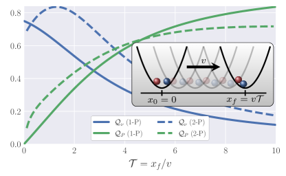
Figure 1: Quality factors $\mathcal{Q}_{\nu}$ and $\mathcal{Q}_{P}$ for velocity and power, respectively, as a function of inverse driving speed $\mathcal{T}=x_{f}/{v}$ for a moving trap. Solid lines (1-P): One particle, $\beta=10.0$, $\mu=1.0$ and $x_{f}={v}\mathcal{T}=10.0$. Dashed lines (2-P): Two interacting particles as shown in the inset. The parameters are given in the Supplemental Material Note (1).

The bound (1) becomes strongest for $\mathcal{T}\ll 1/(\mu k)$, i.e., for observation times smaller than the relaxation time. Remarkably, an estimate that yields up to $\sim 80\%$ of the total entropy production is obtained by just observing the traveled distance of the particle without knowing the strength of the trap. In the slow-driving limit, the dispersion of the velocity becomes negligible, while heat is continuously dissipated into the surrounding medium. As a consequence, the original TUR for a NESS is violated while relation (1) holds due to the additional response term.

Another current to which relation (1) can be applied to is the time-averaged power

$$P(\mathcal{T},{v})=\frac{1}{\mathcal{T}}\int_{0}^{\mathcal{T}}\differential{t}\int\differential{x}p(x,t;{v})\partial_{t}V(x,\lambda({v}t)).$$ (5)

Due to the Gaussian nature of the work fluctuations, it follows that $D_{P}(\mathcal{T},{v})=P(\mathcal{T},{v})/\beta$. Moreover, the entropy production is bounded from above as $\beta P(\mathcal{T},{v})/\sigma(\mathcal{T},{v})\geq 1$ Note (1). Consequently, the TUR for steady-state systems Barato and Seifert (2015); Gingrich et al. (2016) is always violated except in the long-time limit, where the mean power converges to the mean total entropy production rate. In contrast, our result (1) provides a lower bound on the mean total entropy production rate, which, in this case, is obviously quite different from the ordinary TUR.

To illustrate the inequality (1) for a more complex system, we investigate two interacting particles trapped in the harmonic potential (3). We choose a Lennard-Jones interaction between the particles Note (1) and analyze the quality factors for the sum of both particle velocities, i.e., the total traveled distance, and for the power applied to the particles. As shown in Fig. 1, the quality factors are similar compared to the ones for the non-interacting model and reach also about $80\%$.

General set-up for overdamped Langevin dynamics. We consider a system described by an overdamped Langevin equation for the position $x(t)$ in a thermal environment with inverse temperature $\beta$,

$$\partial_{t}x(t)=\mu F(x(t),\lambda({v}t))+\zeta(t),$$ (6)

where $\mu$ denotes the mobility and $\zeta(t)$ is Gaussian white noise with strength $2D\equiv 2\mu/\beta$. The system is driven by a force $F(x,\lambda({v}t))$, which depends on an external protocol $\lambda({v}t)$ that contains a speed parameter ${v}$. The driving starts at $t=0$ with arbitrary initial distribution $p(x,0)$ and runs until $t=\mathcal{T}$. The time evolution of the probability density $p(x,t;v)$ follows the Fokker-Planck equation $\partial_{t}p(x,t;v)=-\partial_{x}j(x,t;v)$ with the probability current

$$j(x,t;v)\equiv\left[\mu F(x,\lambda({v}t))-D\partial_{x}\right]p(x,t;v).$$ (7)

On the level of individual trajectories, we distinguish state variables from (still fluctuating) currents. Specifically, given a function $a(x,\lambda)$, we define an instantaneous state variable as

$$a_{\mathcal{T}}\equiv a(x(\mathcal{T}),\lambda(v\mathcal{T})),$$ (8)

which depends on the final value of position and control. A further observable is its time-averaged variant given by

$$A_{\mathcal{T}}\equiv\frac{1}{\mathcal{T}}\int_{0}^{\mathcal{T}}\differential{t}a(x(t),\lambda(vt)).$$ (9)

The ensemble average of these stochastic quantities will be denoted by $a(\mathcal{T},{v})\equiv\expectationvalue{a_{\mathcal{T}}}$ and $A(\mathcal{T},{v})\equiv\expectationvalue{A_{\mathcal{T}}}$, where we make the dependence on the two crucial parameters explicit.

For time-dependently driven systems there exist two kinds of currents. Both are odd under time-reversal. The first type of current is called a jump current and is of the form

$$J^{\mathrm{I}}_{\mathcal{T}}=\frac{1}{\mathcal{T}}\int_{0}^{\mathcal{T}}\differential{t}d^{\mathrm{I}}(x(t),\lambda({v}t))\circ\dot{x}(t).$$ (10)

Here, $\circ$ denotes the Stratonovich product. The second type is a state current given by

$$J^{\mathrm{II}}_{\mathcal{T}}=\frac{1}{\mathcal{T}}\int_{0}^{\mathcal{T}}\differential{t}d^{\mathrm{II}}(x(t),\lambda({v}t)).$$ (11)

For jump currents, $d^{\mathrm{I}}(x(t),\lambda({v}t))$ is an arbitrary increment, whereas for state currents

$$d^{\mathrm{II}}(x(t),\lambda(vt))\equiv\partial_{t}\lambda({v}t)\partial_{\lambda}b(x(t),\lambda)|_{\lambda=\lambda({v}t)}$$ (12)

involves the derivative of a state function $b(x,\lambda$) with respect to the time-dependent driving. We denote the mean values of these observables by $J^{\mathrm{I}}(\mathcal{T},{v})\equiv\expectationvalue{J^{\mathrm{I}}_{\mathcal{T}}}$ and $J^{\mathrm{II}}(\mathcal{T},{v})\equiv\expectationvalue{J^{\mathrm{II}}_{\mathcal{T}}}$. A prominent example for the first type is the mean rate of entropy production in the medium Seifert (2012)

$$\sigma_{m}(\mathcal{T},{v})\equiv\frac{1}{\mathcal{T}}\int_{0}^{\mathcal{T}}\differential{t}\int\differential{x}\beta F(x,\lambda({v}t))j(x,t;{v})$$ (13)

with increment $d^{\mathrm{I}}(x,\lambda)=\beta F(x,\lambda)$. The mean total entropy production rate

$$\sigma(\mathcal{T},{v})\equiv\frac{1}{\mathcal{T}}\int_{0}^{\mathcal{T}}\differential{t}\int\differential{x}\frac{j^{2}(x,t;{v})}{Dp(x,t;{v})}$$ (14)

additionally contains the entropy production rate of the system Seifert (2012). The power applied to a system as given in eq. (5) belongs to the second type of currents and is obtained by choosing $b(x,\lambda)=V(x,\lambda)$, where $V(x,\lambda)$ is an external potential.

Fluctuations of all these observables can be quantified by the effective diffusion coefficient

$$D_{X}(\mathcal{T},{v})\equiv\mathcal{T}\left(\expectationvalue{X_{\mathcal{T}}^{2}}-\expectationvalue{X_{\mathcal{T}}}^{2}\right)/2$$ (15)

and $X_{\mathcal{T}}\in\{a_{\mathcal{T}},A_{\mathcal{T}},J^{\mathrm{I,II}}_{\mathcal{T}}\}$. For both types of current observables as defined in eqs. (10) and (11), the TUR (1) holds true Note (1).

Uncertainty relation for state variables. Our second main result is a thermodynamic uncertainty relation for end-point and time-integrated state observables as defined in eqs. (8) and (9). For both types of observables, it reads Note (1)

$$[\Delta\mathcal{A}(\mathcal{T},{v})]^{2}/D_{\mathcal{A}}(\mathcal{T},{v})\leq\sigma(\mathcal{T},{v}),$$ (16)

where $\mathcal{A}(\mathcal{T},{v})\in\{a(\mathcal{T},{v}),A(\mathcal{T},{v})\}$. For $a(\mathcal{T},{v})$, this relation shows that a lower bound for the mean total entropy production rate can be obtained by just observing the final state of the system. There is neither information required about the initial distribution nor information about the forces acting on the particle. This bound is especially useful for finite-time or relaxation processes where the total entropy production is not necessarily time-extensive.

Sketch of the proof. To sketch the derivation of our main results (1) and (16) (see Note (1) for a full proof), we use a recently obtained inequality, called the fluctuation-response inequality (FRI), which relates the fluctuations of an observable with its response to an external perturbation Dechant and ichi Sasa (2020). Specifically, for this perturbation we choose the additional force $\epsilon Y(x,t;\epsilon)$ with a parameter $\epsilon$. Averages in the perturbed dynamics are denoted by $\expectationvalue{\cdot}^{\dagger}$. For a small force, i.e., for $\epsilon\to 0$, the FRI bounds the diffusion coefficient (15) for each choice of $X_{\mathcal{T}}$ as Dechant and ichi Sasa (2020); Note (1)

$$D_{X}(\mathcal{T},{v})\geq\frac{\left(\partial_{\epsilon}\expectationvalue{X_{\mathcal{T}}}^{\dagger}|_{\epsilon=0}\right)^{2}}{1/\mathcal{T}\int_{0}^{\mathcal{T}}\differential{t}\expectationvalue{Y(x(t),t;\epsilon)^{2}/D}^{\dagger}|_{\epsilon=0}}.$$ (17)

We choose $Y(x,t;\epsilon)=j(x,t^{\prime};v^{\dagger})/p(x,t^{\prime};v^{\dagger})$, scale time $t^{\prime}=(1+\epsilon)t$ as in Refs. Dechant and Sasa (2018b); Liu et al. (2020), and additionally modify the speed parameter ${v}^{\dagger}={v}/(1+\epsilon)$. The perturbed dynamics then corresponds to a system that evolves slightly slower or faster in time. The denominator in (17) becomes the total entropy production rate $\sigma(\mathcal{T},{v})$. The nominator simplifies to $\Delta\mathcal{A}(\mathcal{T},{v})$ for state variables and to $J^{\mathrm{I,II}}(\mathcal{T},{v})+\Delta J^{\mathrm{I,II}}(\mathcal{T},{v})$ for currents leading to our main results (1) and (16).

Generalization to discrete states: protein folding. Our two main results (1) and (16) hold not only for overdamped Langevin systems but also for systems with discrete states. A paradigm for such a system is a protein undergoing conformational transitions. Experimental studies aim to infer the structure of the underlying Markovian network that possibly contains hidden folded states. For the protein Calmodulin, the transition rates between various folded and unfolded states have been measured as a function of an external force generated by optical tweezers in Ref. Stigler et al. (2011).

We apply our bounds to this system by using these experimental data. In Fig. 2a, the topology of the network consisting of six different conformational states (denoted as in the original paper) is shown. Starting in equilibrium at a constant external force of $f_{0}=9.0$ pN, we drive the system in a force ramp according to the driving protocol $\lambda({v}t)\equiv f_{0}+{v}t(f_{1}-f_{0})$ with $f_{1}=11.0\,\mathrm{pN}$ and ${v}\mathcal{T}=1.0$.

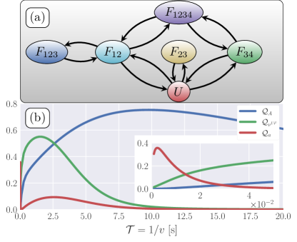
Figure 2: Dynamical unfolding of Calmodulin. (a) Network of its six states, comprising an unfolded state $U$, two partially folded states $F_{12}$ and $F_{34}$, a folded state $F_{1234}$, and two misfolded states $F_{23}$ and $F_{123}$. The force-dependent transition rates between the six states as extracted from Ref. Stigler et al. (2011) are given in the supplemental material Note (1). (b) Three quality factors as defined in the main text as a function of the inverse driving speed $\mathcal{T}=1/{v}$. Inset shows data for fast driving.

For three different observables, we consider the quality factor of the resulting bound on the entropy production associated with this dynamical unfolding. One estimate according to eq. (1) is obtained by observing the current between the unfolded state $U$ and any of the adjacent states $F\in\{F_{12},F_{23},F_{34}\}$,

$$\nu^{UF}_{\mathcal{T}}\equiv[m_{UF}(\mathcal{T})-m_{FU}(\mathcal{T})]/\mathcal{T}.$$ (18)

The variable $m_{UF}$ counts the total number of transitions from the unfolded state $U$ to any of these states $F$ and $m_{FU}$ is the number of reverse transitions. Two further bounds are obtained using $a(i,\lambda)=\delta_{i,F_{12}}$ in eq. (8) and $a(i,\lambda)=\delta_{i,U}$ in eq. (9), which corresponds to the characteristic function of state $F_{12}$ and $U$, respectively . The first choice corresponds to the probability for the protein to be in state $F_{12}$ at the end of the observation time and the latter one to the overall fraction of time the system has spent in the unfolded state $U$. We denote the corresponding quality factors by $\mathcal{Q}_{a}$ and $\mathcal{Q}_{A}$, respectively. The quality factors obtained from monitoring the mean, the fluctuations and the response of these three observables are shown in Fig. 2b. The quality factor $\mathcal{Q}_{A}$ becomes best at slower driving, $\mathcal{T}\simeq 10$, where it yields about $75\%$ of the total entropy production rate. The estimate $\mathcal{Q}_{\nu^{UF}}$ through the current observable is especially strong for intermediate times $1.0\leq\mathcal{T}\leq 2.0$. The quality factor $\mathcal{Q}_{a}$ based on the observation of the final state is always weaker than the other two except for fast driving speeds $\mathcal{T}=1/{v}\sim 10^{-2}$, where it reaches a maximal value of about $40\%$ as shown in the inset of Fig. 2b. Obviously, in future experiments, one should explore the bounds resulting from as many experimentally accessible state and current observables as possible since we do not yet have a criterion for selecting a priori the observable that will yield the strongest bound.

Concluding perspective. We have derived a universal thermodynamic uncertainty relation that holds for current and state variables in systems that are time-dependently driven from an arbitrary initial state over a finite time-interval. The mean and fluctuations of any such observable yields a lower bound on the overall entropy production. Depending on the conditions the observables leading to the relative best bound may change. For observables based on currents, our relation becomes the established ones for the very special cases of time-independent driving, of periodic driving and of relaxation at constant control parameters as summarized in table 1.

Table 1: Unification of TURs with their range of applicability (y=yes, n=no). The factor $\Delta J(\mathcal{T},{v})$ in eq. (1) specialized to NESSs, periodic steady states (PSS) and relaxation (REL) towards equilibrium or a NESS leads to the terms shown on the right-hand sides in the first column. Beyond these known cases, the new relation (1) is applicable for relaxation towards a PSS and for arbitrary time-dependent driving (TTD).

$D_{J}\sigma/J^{2}\geq\Xi$	Ref.	NESS	PSS	REL	TTD
$\Xi=1$	Barato and Seifert (2015); Gingrich et al. (2016)	y	n	n	n
$\Xi=[1+\mathcal{T}\partial_{\mathcal{T}}J/J]^{2}$	Dechant and Sasa (2018a); Liu et al. (2020)	y	n	y	n
$\Xi=[1-\Omega\partial_{\Omega}J/J]^{2}$	Koyuk and Seifert (2019)	y	y	n	n
$\Xi=[1+\Delta J/J]^{2}$	eq.(1)	y	y	y	y

In this sense, our work presents a unifying perspective on extant TURs.

With these relations we have provided universally applicable tools that will allow thermodynamic inference in time-dependently driven systems. We emphasize that it is neither necessary to know the precise coupling between the system and the control nor to know the interactions within the system. It suffices that the experimentalist can change the overall speed of the control slightly and measure the resulting response of an observable. These rather weak demands should facilitate the application to systems beyond colloidal particles and single molecules manipulated with time-dependent optical traps. Finally, as a challenge to theory, it will be intriguing to explore whether and how these relations can be extended to time-dependently driven open quantum systems.

References

- Harada and Sasa (2005) T. Harada and S. I. Sasa, Phys. Rev. Lett. 95, 130602 (2005).
- Toyabe et al. (2010) S. Toyabe, T. Okamoto, T. Watanabe-Nakayama, H. Taketani, S. Kudo, and E. Muneyuki, Phys. Rev. Lett. 104, 198103 (2010).
- Fodor et al. (2016) É. Fodor, W. W. Ahmed, M. Almonacid, M. Bussonnier, N. S. Gov, M.-H. Verlhac, T. Betz, P. Visco, and F. van Wijland, EPL 116, 30008 (2016).
- Lander et al. (2012) B. Lander, J. Mehl, V. Blickle, C. Bechinger, and U. Seifert, Phys. Rev. E 86, 030401(R) (2012).
- Battle et al. (2016) C. Battle, C. P. Broedersz, N. Fakhri, V. F. Geyer, J. Howard, C. F. Schmidt, and F. C. MacKintosh, Science 352, 604 (2016).
- Kawai et al. (2007) R. Kawai, J. M. R. Parrondo, and C. Van den Broeck, Phys. Rev. Lett. 98, 080602 (2007).
- Blythe (2008) R. A. Blythe, Phys. Rev. Lett. 100, 010601 (2008).
- Vaikuntanathan and Jarzynski (2009) S. Vaikuntanathan and C. Jarzynski, EPL 87, 60005 (2009).
- Roldan and Parrondo (2010) E. Roldan and J. M. R. Parrondo, Phys. Rev. Lett. 105, 150607 (2010).
- Muy et al. (2013) S. Muy, A. Kundu, and D. Lacoste, The Journal of Chemical Physics 139, 124109 (2013).