Effective temperatures in inhomogeneous passive and active
bidimensional Brownian particle systems

Abstract

We study the stationary dynamics of an active interacting Brownian particle system. We measure the violations of the fluctuation dissipation theorem, and the corresponding effective temperature, in a locally resolved way. Quite naturally, in the homogeneous phases the diffusive properties and effective temperature are also homogeneous. Instead, in the inhomogeneous phases (close to equilibrium and within the MIPS sector) the particles can be separated in two groups with different diffusion properties and effective temperatures. Notably, at fixed activity strength the effective temperatures in the two phases remain distinct and approximately constant within the MIPS region, with values corresponding to the ones of the whole system at the boundaries of this sector of the phase diagram. We complement the study of the globally averaged properties with the theoretical and numerical characterization of the fluctuation distributions of the single particle diffusion, linear response, and effective temperature in the homogeneous and inhomogeneous phases. We also distinguish the behavior of the (time-delayed) effective temperature from the (instantaneous) kinetic temperature, showing that the former is independent on the friction coefficient.

I Introduction

The out of equilibrium dynamics of macroscopic classical systems attract much theoretical and experimental interest. Basically, there are two ways in which a system can evolve out of equilibrium and break ergodicity: its relaxation times can exceed the measurable time scales, or external and/or internal agents can continuously inject energy and hinder equilibration. Glassy systems pertain to the first class while active matter is, possibly, the most exciting instance of the latter.

In active matter systems the generalized Stokes-Einstein relation between injection and dissipation of energy is violated at the microscopic scale. Energy is thus injected into the samples, they dissipate only part of it, and use the rest to perform directed motion. Numerous review articles report different theoretical and experimental aspects of active matter systems Fletcher and Geissler (2009); Menon (2010); Vicsek and Zafeiris (2012); Ramaswamy (2010); Marchetti et al. (2013); Elgeti et al. (2015); de Magistris and Marenduzzo (2015); Gonnella et al. (2015); Bechinger et al. (2016); Bernheim-Groswasser et al. (2018); Cugliandolo and Gonnella (2019); Carenza et al. (2019); Bär et al. (2020); Löwen (2020).

Recurrent in the analysis of macroscopic out of equilibrium systems is the search for notions borrowed from equilibrium statistical physics and thermodynamics, which could guide one towards a better understanding of their dynamic behaviour. Although essentially out of equilibrium at a microscopic level, the macroscopic character of at least some active matter systems is akin to the one of equilibrium systems in some respects. Moreover, many models of active matter admit a weak energy injection limit in which the evolution occurs close to equilibrium. Consequently, small deviations from the equilibrium Gibbs-Boltzmann measure characterize at least some aspects of the steady state. For these reasons, effective measures for the large scale properties of the stationary state, that are close to equilibrium ones, have been proposed; concerning these features a few relevant references are Tailleur and Cates (2008, 2009); Takatori and Brady (2015); Marconi and Maggi (2015); Fodor et al. (2016); Cagnetta et al. (2017); Han et al. (2017); Solon et al. (2018); Chiarantoni et al. (2020).

A very recent study in this direction is the one of Han et al. Han et al. (2020) who demonstrated that, in a system of active spinners, a single effective temperature enters both the Boltzmann distribution and the equation of state. Notably, the same effective temperature governs the linear response through the Green-Kubo relations for the shear and odd viscosities. However, this is not a finalised story, and some other works show that extreme care has to be taken when trying to use equilibrium-like measures to describe the full behaviour of active (and for that matter also glassy) systems. See, for instance, Solon et al. (2015); Ginot et al. (2015); Guioth and Bertin (2019).

In the study of glassy systems, an effective thermal picture of the large scale dynamics can be exactly derived for mean-field models and it has been applied, quite successfully, to realistic models as well Cugliandolo et al. (1997); Cugliandolo and Kurchan (2000). The notion of an effective temperature defined from the deviations of the fluctuation dissipation theorem (FDT) out of equilibrium has been particularly useful in this regard. One can naturally wonder whether a similar scenario applies to active matter systems, at least for some range of parameters, possibly close to the passive limit.

More precisely, the idea is to measure the effective temperature Cugliandolo et al. (1997); Cugliandolo and Kurchan (2000) as the parameter that replaces the bath temperature in the fluctuation-dissipation relations between the time-delayed correlation and the linear response of the same observables. In practice, one exploits the relation (setting $k_{B}=1$):

$$2T_{\text{eff}}(\Delta t)\chi(\Delta t)=\Delta^{2}(\Delta t)\;,$$ (1)

which relates spontaneous (mean square displacement of, for example, the position of a tagged particle, $\Delta^{2}$) and induced (linear response to a perturbation applied to the position of the same particle, $\chi$) fluctuations. In the long time-delay limit, $\Delta t\gg t^{*}$ with $t^{*}$ some transient scale, many interesting systems presenting collective phenomena, reach a regime in which $T_{\text{eff}}(\Delta t)$ saturates to a constant $T_{\text{eff}}$. Under certain conditions, summarised in the review articles Cugliandolo (2011); Puglisi et al. (2017); Sarracino and Vulpiani (2019), $T_{\rm eff}$ can be interpreted as an effective temperature, measurable with thermometers, controlling the direction and amount of heat flows, partial equilibrations, etc.

Numerical measurements of such effective temperature in different active Brownian interacting systems appeared in Loi et al. (2008, 2011a); Levis and Berthier (2015); Preisler and Dijkstra (2016); Szamel (2017); Nandi and Gov (2018); Cugliandolo et al. (2019); Cengio et al. (2019); Flenner and Szamel (2020) (particles), Loi et al. (2011b, a) (polymers), Suma et al. (2014); Petrelli et al. (2018) (dumbbells). Experimental measurements of the effective temperatures, mainly using tracer particles, were presented in, e.g., Wu and Libchaber (2000); Mizuno et al. (2007); Wilhelm (2008); Gallet et al. (2009); Palacci et al. (2010); Patteson et al. (2015); Maggi et al. (2017); Cao et al. (2020). In living systems, the violation of FDT has been used to characterize the forces generated by, for example, intracellular active processes. In all these cases, the active systems were in their homogeneous fluid phases. The effective temperatures were also considered in simpler effective models in which active homogeneous motion is mimicked by a single particle generalized Langevin equation with memory Szamel (2014); Fodor et al. (2016); Wulfert et al. (2017); Nandi and Gov (2018); Sevilla et al. (2019). The relation between fluctuation theorems and FDT violations was discussed in Zamponi et al. (2005) and, in the context of active matter, some recent studies focused on the relations between the violation of FDT and the entropy production in Active Ornstein-Uhlenbeck particles Fodor et al. (2016); Caprini et al. (2019); Chaki and Chakrabarti (2018) and effective coarse-grained stochastic scalar field theories Nardini et al. (2017). Still, the full analysis of the thermodynamic properties linked to this definition, and whether it really behaves as a temperature, have not been fully explored in the context of active matter systems.

In this paper we focus on a system of active Brownian particles Henkes et al. (2011); Fily and Marchetti (2012); Fily et al. (2014); Redner et al. (2013); Siebert et al. (2017); Digregorio et al. (2018, 2019) with co-existence between dense and dilute phases in two regions of its phase diagram: close to the passive limit and at high levels of activity where it presents Motility Induced Phase Separation (MIPS). We are interested in quantifying the deviations from FDT in a locally resolved fashion and thus characterizing the effective temperature, as defined in Eq. (1), of the two phases. To perform this task, we developed a new local (in real space) analysis that allowed us to classify particles according to the phase they belong to during a prescribed time interval, and to consequently measure, for each phase, the effective temperature using the same protocol of ref. Cugliandolo et al. (2019). We complemented this analysis with a detailed theoretical and numerical characterization of the per-particle distributions of the displacement, the linear response, and the effective temperature. In particular, the displacement fluctuations were considered (mostly using tracers as the measuring means) in several experiments of active matter systems Wu and Libchaber (2000); Howse et al. (2007); Leptos et al. (2009); Valeriani et al. (2011); Ortlieb et al. (2019); Klongvessa et al. (2019); Lagarde et al. (2020), while the other two distributions are new to this field, though they have been studied in the context of coarsening and glassy systems Castillo et al. (2002, 2003); Romá et al. (2007); Annibale and Sollich (2009); Corberi and Cugliandolo (2012). Connections and differences with theories for dynamic fluctuations in glassy systems will be discussed Chamon and Cugliandolo (2007). At the end the paper, we also briefly discuss the differences between the effective temperature and the kinetic temperature, providing evidences for the differences between these two objects, which access dynamics at completely different time-scales. More arguments on this topic can be found in Ref. Cugliandolo et al. (2019).

The paper is organized as follows. In Sec. II we give the details of the model and the analytical and numerical tools employed. In Subsec. II.1 we briefly describe the Active Brownian Particle (ABP) model and its phase diagram. Subsection II.2 contains the definitions of the mean square displacement, integrated linear response and time-delay dependent effective temperature. Subsection II.3 presents the analytic results for a single ABP that will be used as a reference in the small packing fraction limit. Subsec. II.4, explains the Malliavin auxiliary variables numerical method for the evaluation of linear responses. Next, we present our results. Section III is devoted to the analysis of the globally averaged diffusive and response properties. In particular, in Subsec. III.1 we focus on the dynamics in the active homogeneous liquid phase, while Subsec. III.2 is dedicated to the dynamics in the inhomogeneous cases, both close to the passive limit and in MIPS. In the latter case, we study the dynamical properties and the effective temperature of the two phases separately finding strong heterogeneities, hidden by global measurements over all the particles. The fluctuations of individual displacement, response and effective temperature are studied in great detail in Sec. IV. We present some analytical results for the distributions for a single passive and active particle together with numerical results both in dense homogeneous and heterogeneous passive and active systems. A short Sec. V distinguishes the behavior of the effective temperature from the one of the instantaneous kinetic temperature. We close the paper with a discussion Section in which we summarize our results.

II Methods

In this Section we give details on the numerical model we use and on the protocol we adopt to perform the measurements. We will first recall, in Subsec. II.1, the definition of the ABP model and its phase diagram in the plane packing fraction vs. Péclet number. We will also provide some details on the numerical method and the parameters used. In Subsec. II.2 we will define the observables chosen to study the dynamics and in Subsec. II.3 we will summarize the known analytical results for the mean square displacement, the response function and the effective temperature of a single active Brownian particle. Finally, in Subsec. II.4 we will shortly describe the Malliavin weight sampling technique for the calculation of linear responses with simulations of unperturbed systems.

II.1 The model

We consider a system of $N$ identical active Brownian disks (ABPs) with mass $m$ and diameter $\sigma_{\rm d}$, confined inside a square box with area $A$ and periodic boundary conditions. Their dynamics are described by the Langevin equations:

$$m\ddot{\mathbb{r}}_{i} = -\gamma\dot{\mathbb{r}}_{i}+\mathbb{F}^{\lambda}_{i}+\mathbb{F}^{\text{int}}_{i}+F_{\text{act}}\mathbb{n}_{i}+\sqrt{2\gamma T}\bm{\xi}_{i}\;,$$ (2)

$$\dot{\theta}_{i} = \sqrt{2D_{\theta}}\eta_{i}\;.$$ (3)

($k_{B}=1$ hereafter). ${\mathbb{r}_{i}}$ is the position of the $i$-th particle in the two dimensional space. The particle system is supposed to be in contact with an environment that produces the friction force in the first term in the right-hand-side of Eq. (2) and the one in the left-hand-side of Eq. (3), with $\gamma$ the friction coefficient. ${\mathbb{F}^{\lambda}_{i}}$ is an applied external force depending on a parameter ${\lambda}$. ${\mathbb{F}_{i}^{\text{int}}=-\nabla\sum_{j(\neq i)}U(r_{ij})}$ is the force on the $i$-th particle due to the excluded volume repulsive interactions with all other particles. ${r_{ij}=|\mathbb{r}_{i}-\mathbb{r}_{j}|}$ is the inter-particle distance and $U$ is a short-ranged repulsive potential of the form $U(r)=\left\{4\epsilon[(\sigma/r)^{64}-(\sigma/r)^{32}]+\epsilon\right\}\theta(2^{1/32}\sigma-r)$, with ${\sigma}$ and ${\epsilon}$ the parameters that set the length and energy scales of the interactions, and $\sigma_{\rm d}=2^{1/32}\sigma$. The self-propulsion is modelled as a constant magnitude force $F_{\text{act}}$ along ${\mathbb{n}_{i}=(\cos\theta_{i},\sin\theta_{i})}$. ${\bm{\xi}_{i}}$ and ${\eta_{i}}$ are uncorrelated zero-mean and unit variance Gaussian noises. Henceforth we will indicate the noise averages with angular brackets $\langle\dots\rangle$. One can easily check that the global angular diffusion is characterised by the diffusion coefficient ${D_{\theta}=3T/(\gamma\sigma_{\rm d}^{2})}$. We will express all relevant physical quantities in terms of mass, length and energy units given by m, ${\sigma}$ and ${\epsilon}$, with the reference time unit being $\tau=\sqrt{m\sigma^{2}/\epsilon}$.

We vary the packing fraction, ${\phi=\pi\sigma_{\rm d}^{2}N/(4A)}$, and the Péclet number, ${\text{Pe}=F_{\text{act}}\sigma_{\rm d}/T}$, that measures the strength of the work performed by the activity with respect to the thermal energy scale, while we keep all other parameters fixed. Concretely, we fix $\sigma_{\rm d}=1$ and $T=0.05$. We mainly use $\gamma=10$, which ensures the overdamped limit, but we also study how the friction coefficient affects the effective and kinetic temperatures. Typically, we collect data from systems with $N=256^{2}$ particles and we use 25-75 independent runs to construct the averages and probability distribution functions.

We used a velocity Verlet algorithm for solving Newton’s equations with an additional force term for the Langevin-type thermostat. In order to efficiently parallelize the numerical computation, we used the open source software Large-scale Atomic/Molecular Massively Parallel Simulator (LAMMPS), available at github.com/lammps Plimpton (1995).

We study the dynamic behaviour of the system in different regions of the phase diagram. The latter has been established in Digregorio et al. (2018, 2019) under similar conditions and we reproduce it in Fig. 1. The phases are represented with different colors and they correspond to the liquid (white), the hexatic (blue), the co-existence region between hexatic and liquid (in grey at the left end of the diagram), the solid (orange) and the Motility Induced Phase Separation (MIPS) region (in grey at the right end of the diagram). The vertical straight lines, added to the phase diagram, represent the paths along which we vary the parameters in order to study the effective temperature, namely, by changing $\phi$ at fixed Pe. The colour code (online) will be the same in all figures.

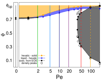
Figure 1: (Color online.) The phase diagram of the ABP model at fixed temperature, $T=0.05$, in lin-log scale, as a function of two adimensional parameters: the Péclet number Pe and the packing fraction $\phi$ Digregorio et al. (2018). The white, blue and orange regions represent the liquid, hexatic and solid phases, respectively. The grey zone at the left end is the co-existence region between hexatic and liquid, while the one at the right end is the region with Motility Induced Phase Separation (MIPS). The lines and points at the border between the different phases have been obtained from the study of the hexatic and positional order correlation functions, the equation of state (EOS) and the bimodal distribution function of the local density, as written in the key. The vertical lines indicate the directions along which we vary $\phi$, at fixed Pe, in order to study the system’s effective temperature.

II.2 Mean-squared displacement, linear response, and the fluctuation dissipation theorem

The most usual way of testing the stochastic dynamics of an interacting system is to evaluate its global mean-square displacement. Focusing on a tagged particle, say the $i$th one, the displacement induced by a given noise realisation is

$$\tilde{\Delta}_{i}(t,0)=\mathbb{r}_{i}(t)-\mathbb{r}_{i}(0)\;,$$ (4)

with $\mathbb{r}_{i}(t)$ and $\mathbb{r}_{i}(0)$ the positions of the selected particle at times $t$ and $0$, respectively. Henceforth we will assume that the system reached a steady state and that the time $0$ is any reference time during this stationary regime. The mean square displacement of the $i$th particle over the time interval $[0,t]$ is then given by the noise average of the above definition,

$$\Delta^{2}_{i}(t,0)=\langle[\mathbb{r}_{i}(t)-\mathbb{r}_{i}(0)]^{2}\rangle\;,$$ (5)

and the global mean square displacement by the normalized sum over al particles, $\Delta^{2}=N^{-1}\sum_{i=1}^{N}\Delta_{i}^{2}$.

Another less usual way of studying the dynamics of a collective system is to measure its response to weak perturbations. Such a procedure is put in practice, for example, by applying a constant perturbation ${\mathbb{F}^{\lambda}_{i}}$, say since ${t=0}$, and then measuring the averaged linear response of the system to it. More precisely, one defines the instantaneous linear self response

$$R_{i,\alpha\beta}(t,t^{\prime})=\left.\frac{\delta\langle{r_{i,\alpha}(t)\rangle_{\mathbb{F}^{\lambda}}}}{\delta F_{i,\beta}^{\lambda}(t^{\prime})}\right|_{\mathbb{F}^{\lambda}=0}$$ (6)

where $\alpha$ and $\beta$ are coordinate indices running from $1$ to $d$, with $d$ the space dimension. The time-integrated linear response is then

$$\chi_{i,\alpha\beta}(t,0)=\int_{0}^{t}dt^{\prime}\;R_{i,\alpha\beta}(t,t^{\prime})\;,$$ (7)

the self contributions averaged over all spatial directions is

$$\chi_{i}(t,0)=\int_{0}^{t}dt^{\prime}\;\sum_{\alpha=1}^{d}R_{i,\alpha\alpha}(t,t^{\prime})\;,$$ (8)

and the global function is the average over all particles $\chi(t,0)=N^{-1}\sum_{i=1}^{N}\chi_{i}(t,0)$. A noise-dependent fluctuating quantity, the average of which yields the linear response in Eq. (8), will be identified in Sec. II.4.

In equilibrium, the mean square displacement and the mean integrated linear response are related by the model independent equation

$$2T\chi_{i}(t,0)=\Delta_{i}^{2}(t,0)\;,$$ (9)

that states the fluctuation-dissipation theorem (FDT).

Since the dynamics of this problem can be heterogeneous, with different particles behaving differently over the time interval considered, $\chi_{i}$ and $\Delta^{2}_{i}$ could have time variations that depend strongly on the particle considered. Still, under equilibrium conditions the relation above should remain particle independent.

II.3 A single active Brownian particle

In the numerical analysis of the linear response function we apply a force along the $x$ direction of space and we focus on the linear response of the system along this direction. Concerning the mean-square displacement, we measure it according to the definition in Eq. (5), that is to say, by summing over all directions of space, which yields, on average, $\Delta_{i}^{2}(t,0)=\langle[\mathbb{r}_{i}(t)-\mathbb{r}_{i}(0)]^{2}\rangle=d\langle[x_{i}(t)-x_{i}(0)]^{2}\rangle$. For this reason, there will be some unusual $d$ factors in the relations appearing in the rest of this paper. They take care of the different ways of calculation linear responses and displacements. In this Section we use the same protocol.

For a single active Brownian particle a straightforward calculation leads to the integrated linear response along one spatial direction

$$\chi(t,0)=\frac{t}{\gamma}\equiv\mu_{\rm sp}t,\;,$$ (10)

with $\mu_{\rm sp}$ the single particle mobility. The mean square displacement reads

$$\Delta^{2}(t,0)=\frac{2}{D_{\theta}^{2}}\frac{F_{\text{act}}^{2}}{\gamma^{2}}\;\left(D_{\theta}t+e^{-D_{\theta}t}-1\right)+\frac{4T}{\gamma}\,t\;,$$ (11)

where we have taken into account the $d=2$ factor, and in the long time limit it approaches the normal diffusion form

$$\Delta^{2}(t,0)\to 2dD_{\rm sp}t\;,$$ (12)

with the single particle diffusion coefficient

$$D_{\rm sp}=\frac{T}{\gamma}\left(1+\frac{\text{Pe}^{2}}{6}\right)\;.$$ (13)

The effective temperature of a single active Brownian particle is then immediately derived by taking the asymptotic value of the ratio between displacement and response

$$T_{\rm eff} = \frac{\lim_{t\gg 1}\Delta^{2}(t,0)}{2d\chi(t,0)}=\frac{D_{\rm sp}}{\mu_{\rm sp}}$$ (14)

$$= T\left(1+\frac{\text{Pe}^{2}}{6}\right)\;.$$

II.4 Malliavin weights

In simulations, it can be very hard to control the vanishing perturbation limit needed to calculate the linear response function. Fluctuations and numerical errors become increasingly large as the perturbation approaches zero. For this reason, techniques that allow one to calculate linear responses with simulations of the unperturbed system only have been developed for some kinds of systems. The trick is to find an exact relation between the linear response and a correlation between some variables evaluated in the unperturbed system that could be, though, complicated (even non-local in time) but still manageable. The advantage of these methods is that the zero perturbation limit is taken analytically and it does not introduce strong numerical uncertainties. Such methods were introduced by Chatelain Chatelain (2003) and Ricci-Tersenghi Ricci-Tersenghi (2003) for Ising spin systems evolving with Monte Carlo dynamics. These ideas were then generalised by Corberi et al. Corberi et al. (2010) to treat similar systems evolving in discrete time via a stochastic non-equilibrium Markov process. Other relations of this kind, though not necessarily presented with the aim of simplifying the numerical computation of the linear response, can be found in Cugliandolo et al. (1994); Gradenigo et al. (2012); Speck (2016); Maes (2019); Cengio et al. (2019) to cite a few papers where these ideas were explored.

Lately, Warren and Allen Warren and Allen (2012, 2014) presented a similar approach for interacting Brownian particles of the type we are dealing with here. The method involves tracking, in an unperturbed system, auxiliary stochastic variables, termed Malliavin weights. More recently, Szamel Szamel (2017) applied it to systems of active particles propelled by a persistent (colored) noise and interacting via a screened Coulomb potential. We have already used this method in a preliminar study of active Brownian disks Cugliandolo et al. (2019).

For the model and perturbation considered in this paper, the Malliavin weights sampling (MWS) technique is particularly simple. It consists in evaluating the correlator between the position of the particle and the thermal white noise acting on it. Indeed, denoting by ${P(\{\mathbb{r}_{i}\};t)}$ the joint probability distribution function (pdf) of all particles’ positions, one defines

$$Q_{\lambda}(\{\mathbb{r}_{i}\};t)\equiv\frac{\partial\ln P(\{\mathbb{r}_{i}\};t)}{\partial\lambda}\;,$$ (15)

with ${\lambda}$ the strength of the perturbation. Next, one introduces the “Malliavin weight”, that is to say an auxiliary stochastic variable, ${q_{\lambda}}$ and lets it evolve, starting from ${q_{\lambda}=0}$, according to the rule

$$q_{\lambda}(t^{\prime})=q_{\lambda}(t)+\frac{\partial\ln W(\{\mathbb{r}^{\prime}_{i}\};t^{\prime}|\{\mathbb{r}_{i}\};t)}{\partial\lambda}\;,$$ (16)

where ${W(\{\mathbb{r}^{\prime}_{i}\};t^{\prime}|\{\mathbb{r}_{i}\};t)}$ is the propagator, i.e. the probability of finding the particles at the positions ${\{\mathbb{r}^{\prime}_{i}\}}$ at ${t^{\prime}=t+\Delta t}$ given the positions ${\{\mathbb{r}_{i}\}}$ at $t$. Given the previous updating rule, it is then readily shown that $\langle q_{\lambda}\rangle_{\{\mathbb{r}_{i}\}}=Q_{\lambda}(\{\mathbb{r}_{i}\};t)$ Warren and Allen (2012). Let ${A(\{\mathbb{r}_{i}\})}$ be a generic function of the coordinates. Its response to a change of $\lambda$ is given by its average, in the unperturbed system, weighted by the appropriate ${q_{\lambda}}$:

$$\frac{\partial\langle A\rangle_{\lambda}}{\partial\lambda}=\langle Aq_{\lambda}\rangle\;.$$ (17)

In general, one cannot calculate the exact propagator but this method can still be applied numerically, by enforcing the relation (16) at each time-step with an explicit integration scheme. If we integrate the equations of motion using a standard Euler-Maruyama scheme, the propagator reads

$$W(\{\mathbb{r}^{\prime}_{i},\theta^{\prime}_{i}\};t^{\prime}|\{\mathbb{r}_{i},\theta_{i}\};t)=\Big{[}(2\pi)^{3}\left(\frac{2T}{\gamma}\right)^{2}2D_{\theta}(\Delta t)^{3}\Big{]}^{-N/2}\;$$

$$\qquad\times\;\prod_{i=1}^{N}\exp\Bigg{\{}-\frac{(x^{\prime}_{i}-x_{i}-\frac{F_{\text{act}}}{\gamma}\cos\theta_{i}\Delta t-\frac{F_{i,x}^{\text{int}}}{\gamma}\Delta t-\frac{F_{i,x}^{\lambda}}{\gamma}\Delta t)^{2}}{2\frac{2T}{\gamma}\Delta t}-\frac{(y^{\prime}_{i}-y_{i}-\frac{F_{\text{act}}}{\gamma}\sin\theta_{i}\Delta t-\frac{F_{i,y}^{\text{int}}}{\gamma}\Delta t-\frac{F_{i,y}^{\lambda}}{\gamma}\Delta t)^{2}}{2\frac{2T}{\gamma}\Delta t}$$

$$\qquad\qquad\qquad\quad\;\;-\frac{(\theta^{\prime}_{i}-\theta_{i})^{2}}{2D_{\theta}\Delta t}\Bigg{\}}$$ (18)

and we just need to let the Malliavin weight evolve according to Eq. (16) using the expression in Eq. (18) for the propagator. For ${\mathbb{F}_{i}^{\lambda}=\lambda\mathbb{e}_{x}}$ one deduces

$$q^{\prime}_{\lambda}=q_{\lambda}+\frac{x^{\prime}_{i}-x_{i}-\frac{F_{\text{act}}}{\gamma}\cos\theta_{i}\Delta t-\frac{F_{i,x}^{\lambda}}{\gamma}\Delta t-\frac{F_{i,x}^{\text{int}}}{\gamma}\Delta t}{2T}\frac{\partial F^{\lambda}_{i,x}}{\partial\lambda}=q_{\lambda}+\sqrt{\frac{\Delta t}{2\gamma T}}\,\omega_{i}^{x},$$ (19)

where ${\omega_{i}^{x}}$ are the normal random variables with expected value zero and unit variance used in the algorithm to simulate the noise. Notice that all the derivatives with respect to $\lambda$ are evaluated at $\lambda=0$, corresponding to the unperturbed evolution. Finally,

$$\chi_{i}(t,0) = \frac{\partial\langle x_{i}(t)\rangle_{\lambda}}{\partial\lambda}=\langle x_{i}(t)q_{\lambda}(t)\rangle$$ (20)

$$= \frac{1}{{\sqrt{2\gamma T}}}\int_{0}^{t}dt^{\prime}\,\langle x_{i}(t)\xi_{i,x}(t^{\prime})\rangle\;,$$

in terms of a correlation with the noise, that we wrote in continuous time notation. Therefore, for the model and perturbing forces considered here, the Malliavin weights sampling technique reduces to the evaluation of the correlation between the position of the tagged particle and the thermal noise acting on it. In practice, we imagine that the perturbation is acting on each particle and we evaluate ${\chi}$ considering an average over the selected particles we will be interested in. In heterogeneous cases we will implement a method to distinguish those in dilute and dense phases and we will study them separately.

Besides, we will be interested in studying the spatial fluctuations of the particle displacement and the quantity

$$\tilde{\chi}_{i}(t,0)=\frac{1}{\sqrt{2\gamma T}}\int_{0}^{t}dt^{\prime}\,x_{i}(t)\xi_{i,x}(t^{\prime})$$ (21)

that, once averaged and time integrated, gives rise to the linear susceptibility.

III Global properties

In this Section we study the globally averaged diffusive and response properties of the ABP model defined in Subsec. II.1, and we compare them to the equilibrium limit. We start our analysis in the homogeneous region of the phase diagram, Subsec. III.1. In Subsec. III.2 we move to the coexisting regions, either in the passive limit or within the MIPS sector. In the latter cases we separate the particles which belong to the dense phases from the ones belonging to the dilute phases and we find evident heterogeneities which are hidden when flat global averages are performed.

III.1 Homogeneous phases

(a)                                       (b)

(c)                                       (d)

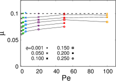
Figure 2: (Color online.) Homogeneous liquid phase. Global (a) mean squared displacement, in log-log scale, and (b) integrated linear response function as a function of delay time for packing fraction $\phi=0.200$ and Péclet values Pe = 0, 2, 5, 20, 50, plotted with the line code given in the key, see also Fig. 1 where this Pe values are indicated as vertical lines with the same color. The diffusion constant (c) and mobility (d) as a function of the packing fraction $\phi$ for six different values of Pe, see the key in panel (b). The dashed lines are the single particle behavior and the key to the datapoints is in panel (d). The data shown in panel (c) are fitted using a quadratic function, while the solid line in panel (d) are guides to the eye. (Some points are missing because for $\phi=0.200,\ 0.250$ and Pe = $100$ the system is already in the MIPS region.)

As long as we stay in the homogeneous liquid phase, both the global mean square displacement, shown in Fig. 2(a) for $\phi=0.2$, and the global linear response, shown in Fig. 2(b) for the same $\phi$, increase with increasing Péclet number, and slow down when the density is increased. At the low densities of this plot, the dynamics reach a normal diffusive regime and in Fig. 2(c)-(d) we see that both the diffusion coefficient (defined through the long-time limit of the mean squared displacement $D=\lim_{t\gg 1}\Delta^{2}(t,0)/(2dt)$) and the mobility (defined as $\mu=\lim_{t\gg 1}\chi(t,0)/t$) decrease when the packing fraction is increased for all values of the Péclet number such that the system remains in the homogeneous liquid phase. The combination of these behaviors also results in a decrease of the effective temperature with increasing packing fraction. These claims were already shown in Cugliandolo et al. (2019) and are supported by the numerical data displayed in Figs. 2 and 3. In the latter, the parametric construction $\chi(\Delta^{2})$ is presented in the main plot of panel (a) for Pe = 20 and several packing fractions. Extracting the effective temperature from these measurements, one sees that after a transient with a non-trivial dependence on the time delay, there is a time scale beyond which $T_{\rm eff}$ saturates to a constant, see the inset of the same panel, where the effective temperatures measured from the long time limit, and normalized by the effective temperature at Pe = 0, are shown. The dependence of this long-time value on the packing fraction of the system is displayed in Fig. 3(b). The effective temperature is a monotonic decreasing function of the global density (a similar trend was found in Levis and Berthier (2015)).

Nandi and Gov proposed a simple picture for the long-term dynamics of active systems, in which the behaviour of the global system is reduced to the one of a single active particle inside a visco-elastic fluid, that leads to a dependence of the effective temperature of the form $A/(1+B\phi^{2})$ Nandi and Gov (2018). Although our numerical data are compatible with this form, they are also rather well described by pure linear decays, and it is hard to establish beyond doubt which of the two functions describes more accurately the intermediate packing fraction behaviour, $\phi\stackrel{{\scriptstyle<}}{{\sim}}0.5$, that we study here.

The curves in Fig. 3(b) tend to 1 at vanishing packing fraction indicating that for dilute enough systems $T_{\rm eff}$ grows as Pe² similarly to what was found in Loi et al. (2008, 2011b, 2011a) for other interacting active particle and molecular models, and in Suma et al. (2014) for an active dumbbell system. This dependence is conserved at finite relatively low density as can be guessed from the Pe² dependence of the diffusion coefficient and almost constant behavior of the mobility shown in Fig. 2.

(a)                                                

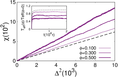
(b)                                                

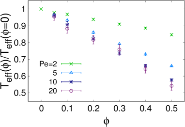
Figure 3: (Color online.) Homogeneous liquid phase. (a) The global integrated linear response function vs. the mean squared displacement (main plot) and the effective temperature normalized by the one of a single active particle (inset) for Pe = $20$ and the packing fractions values given in the key. The dashed line is the single particle behavior. (b) The long-time effective temperature vs. the packing fraction for the activities given in the key.

III.2 Inhomogeneous phases

When entering the coexisting regions, either between the fluid and the hexatically ordered phase at low Pe, or within the MIPS sector of the phase diagram at high Pe, the scenario becomes richer and more complex. On the one hand, we can perform global averages over all particles, be them in dense or dilute regions of the sample. On the other hand, we can go beyond these naive measurements and differentiate the dynamics of the two phases separately.

More precisely, we will demonstrate that one can attribute a dilute/dense character to the particles, over a chosen time interval, and that these behave as if they were characterized by two different effective temperatures. The latter fact is hidden when flat global averages are performed. We will then compare this kind of heterogeneities to the ones already studied in different glassy materials.

III.2.1 Method for particle distinction

In heterogeneous systems, we proceed as follows to separate the particles in two groups. First of all, we evaluate the hexatic local order parameter, $\psi_{6i}=(1/N^{i}_{nn})\sum_{j(i)}e^{6{\rm i}\theta_{ij}}$ where $\theta_{ij}$ is the angle formed by the bond between the selected particle $i$ and its first neighbor $j$, and a reference axis, say the horizontal one. It is clear that, in order to define these bonds, a notion of neighborhood needs to be introduced. This is done by performing a Voronoi tessellation of space. The sum $\sum_{j(i)}$ runs over nearest neighbors ($N^{i}_{nn}$ in total), in the Voronoi sense, of the selected particle. In this way, each particle acquires a vector $\psi_{6i}$ that is attached to it. Next, we perform a time-average of the absolute value of the local hexatic order parameter over a time window of duration $\Delta t$, $(1/\Delta t)\,\int_{t}^{t+\Delta t}dt^{\prime}\,|\psi_{6i}(t^{\prime})|$. The statistics of the thus constructed mean local hexatic order parameter shows a bimodal structure. We use the central minimum of the probability distribution function, located between the two local maxima, to separate the particles in two subgroups: the ones which spent most of their lifetime $\Delta t$ in the dilute phase and those which spent most of their lifetime $\Delta t$ in the dense phase.

(a)                                     (b)

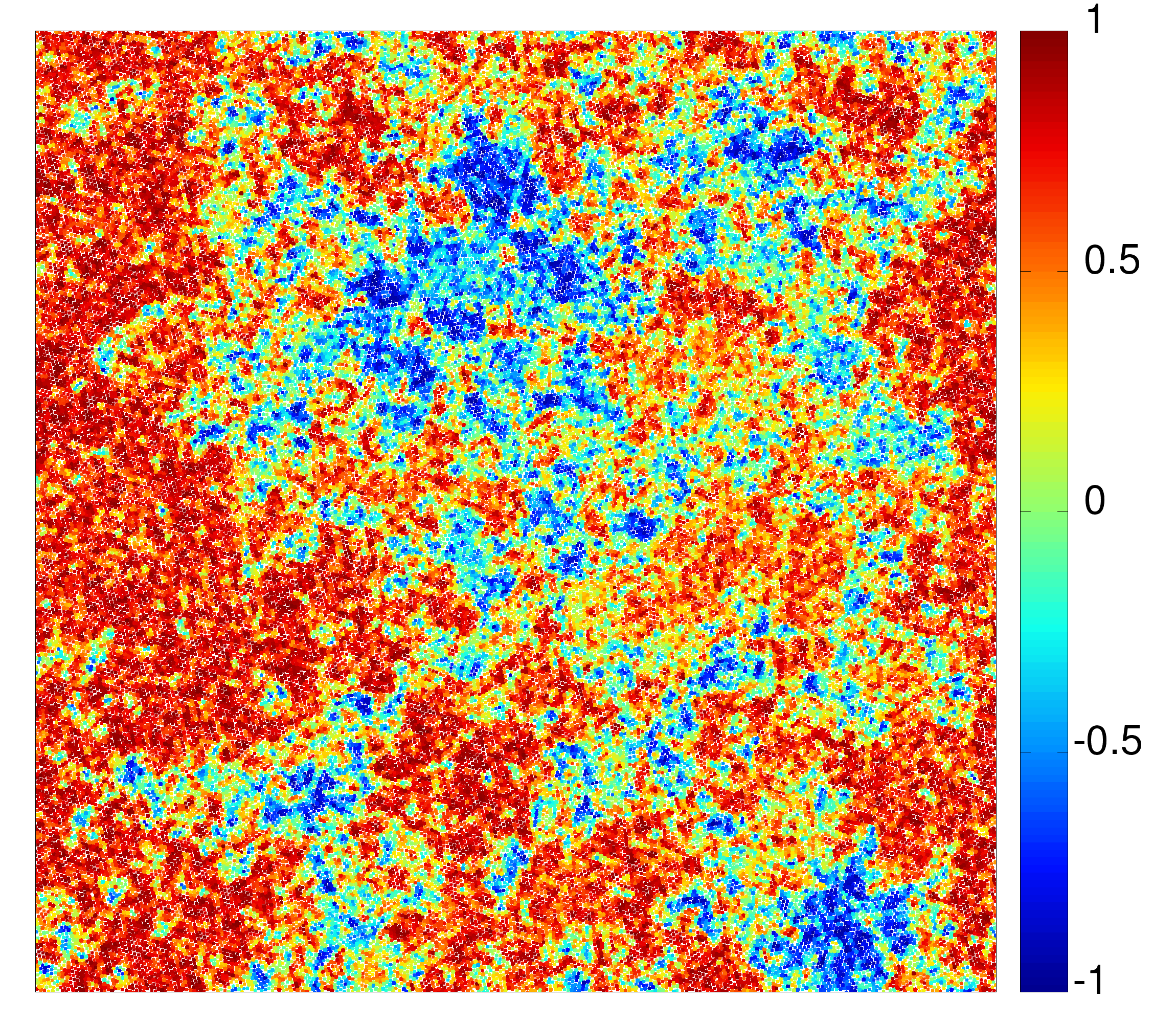
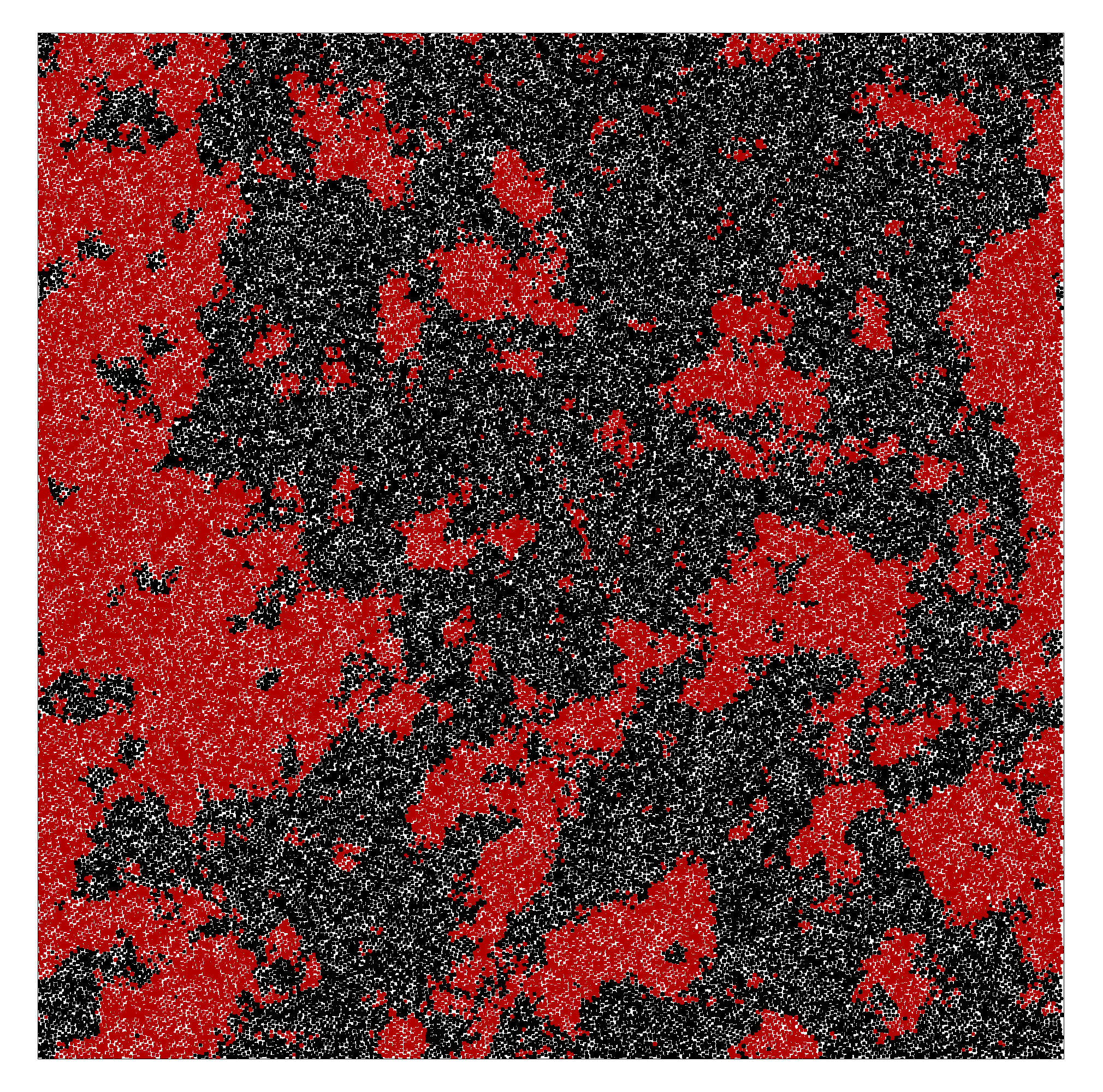
(c)                                                       

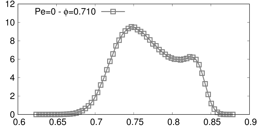
Figure 4: (Color online.) Example of particle classification in a passive system (Pe = 0) in the coexistence region, $\phi=0.71$. (a) Map of local hexatic order parameter at a given time $t$ within the measuring interval $\Delta t$, projected on the direction of its global average. Particles painted red have unit projection on the average value and the rest of the colour code is given by the right vertical bar where the numerical values are the outcome of this projection. (b) Particles in the dense phase are painted red and those in the dilute phase are colored black, as identified using the criterium explained in the main text. In this case $\Delta t=10^{3}$. (c) Bimodal probability distribution function of the hexatic order parameter averaged over $\Delta t=10^{3}$.

We show an example of this construction in Fig. 4. In panel (a) we present the map of the instantaneous local hexatic order parameter with the convention that red corresponds to the average hexatic direction (in complex space) and blue to the one opposed to it (the hexagonal lattice is rotated by $\pi/6$ with respect to the one of the dark red regions), with the scale given next to the plot for the intermediate directions. In general, regions of the same color identify clusters having the same hexatic value. This is the convention used in Digregorio et al. (2018, 2019). In (b) we show which particles belong to the dense cluster (red) or the dilute phase (black) after an averaging time of $\Delta t=10^{3}$, using the criterion described above. We see a correlation with the instantaneous map in panel (a) although it is not perfect, because of the time average. In panel (c) we show the probability distribution function of the hexatic order parameter averaged over the same time interval.

III.2.2 The passive case

We have explained the method that we use to identify the particles that, on the one hand, were and stayed in the dense/hexatically ordered clusters, and the ones that, on the other hand, were and stayed in the dilute/disordered phase, between two selected times.

(a)

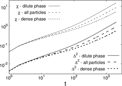
(b)

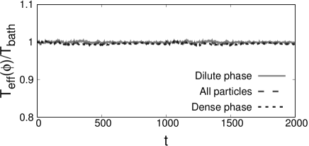
Figure 5: (Color online.) Passive inhomogeneous system. ${\text{Pe}=0}$ and ${\phi=0.710}$. (a) Time-delay dependence in log-log scale of the mean square displacement (thick lines) and integrated linear response (thin lines) calculated by averaging over the particles which spent enough time in the gaseous phase (solid), in the cluster phase (dotted) or over all particles in the system (dashed). (b) Effective temperature normalized by the temperature of the bath calculated considering all the particles (dashed), only the ones belonging to the dense phase (dotted) or to the dilute phase (solid).

As already explained, in Fig. 4 we show an example of the outcome of this classification in a passive system with coexistence. Concretely, we show data for ${\text{Pe}=0}$ and ${\phi=0.710}$ in order to be approximately in the middle of the coexistence region. From Fig. 5, we infer that even though the mean square displacement and the integrated linear response of the particles in the dense and dilute phases are very different, the effective temperature of both is the same (within numerical errors). Consistently with the expectations, since the system is in thermal equilibrium, the effective temperature is homogeneous and it equals the temperature of the bath at all time delays, even when the displacement and linear response show non-trivial time-dependencies.

III.2.3 The active case

Close to the passive limit Pe = 0, in a very narrow region of the phase diagram, the co-existence between hexatic and liquid phases survives. It is, however, quite difficult to see the effects of activity here, since the Pe values are very small and their effect is very weak. Data are not considerably different from the ones in the passive case. We do not show them here.

Once strong activity is applied, the system has the possibility of undergoing MIPS in between two limiting packing fractions, say $\phi_{<}({\rm Pe})$ and $\phi_{>}({\rm Pe})$. In MIPS, two sets of particles can be identified, those in the gaseous phase and those in dense cluster, the former with packing fraction $\phi_{<}$ and the latter with packing fraction $\phi_{>}$.

(a)                                     (b)

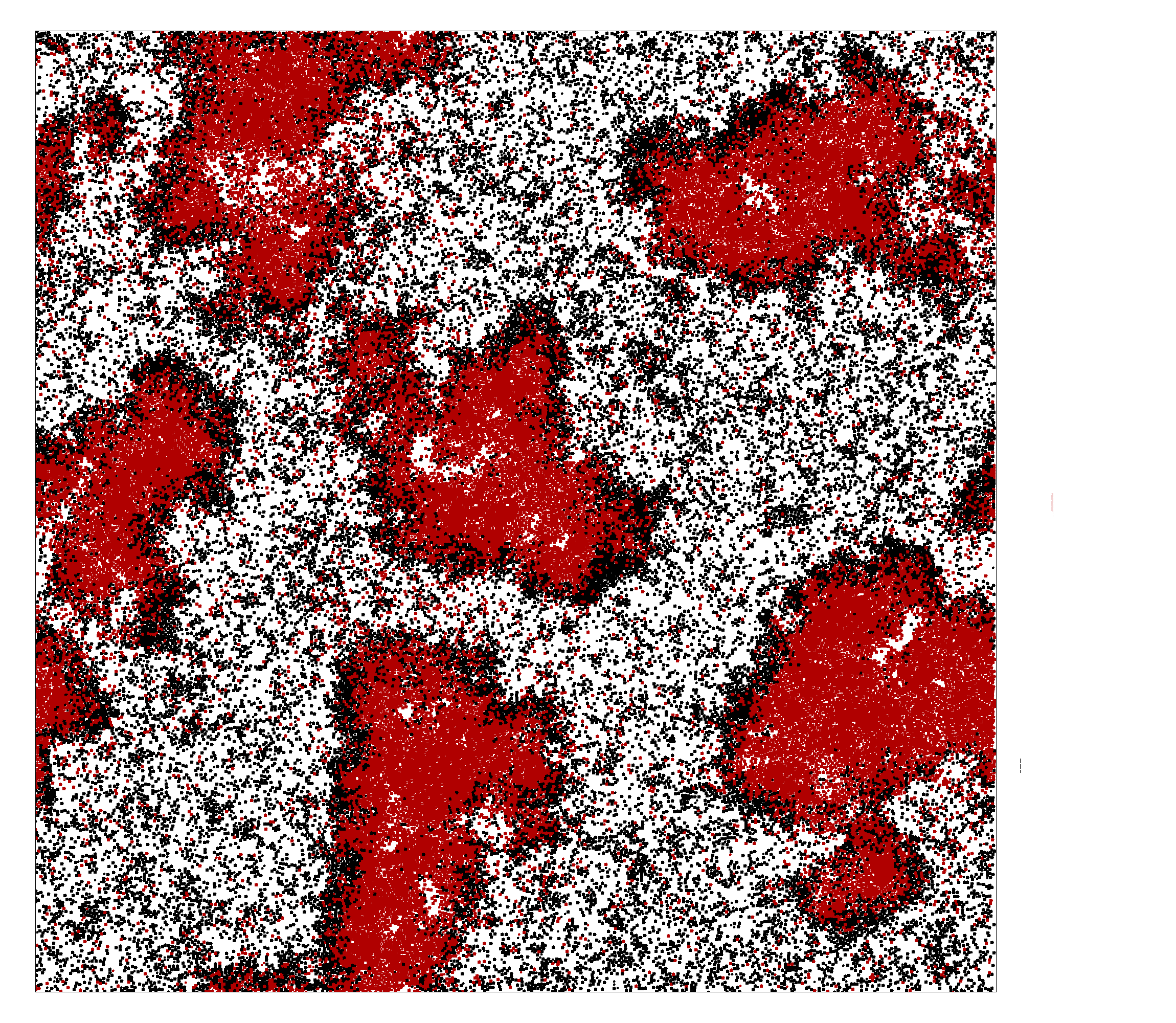
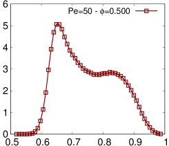
Figure 6: (Color online.) Example of particle classification in the MIPS phase, $\phi=0.5$ and Pe = 50. (a) Particles coloured red (black) belong to the dense (dilute) phase during the time interval $\Delta t=10^{3}$. The configuration is taken at the end of the measuring time: most of particles at the interfaces are coloured in black because either the instantaneous value of the hexatic parameter is lower than the chosen threshold to separate the cluster or they have not spent enough time in the dense region to be considered belonging to it. (b) Probability distribution function of the averaged hexatic order parameter.

The separation of the particles according to whether they mostly belong to the dilute or dense phase during a pre-defined time-interval, looks like what is shown in Fig. 6. In panel (a) we show a typical configuration of the system: the particles which spent most of their lifetime in the dense phase are depicted in red, while the particles of the dilute phase are depicted in black. Panel (b) illustrates the criterium used to separate the particles in the two groups. The pdf of the hexatic order parameter averaged over a time interval $\Delta t=10^{3}$ is bimodal and we chose its minimum as the threshold to separate the particles in the two phases. In Fig. 7 we show the mean square displacements and linear responses that lead to the effective temperatures in the two phases. First of all, we note that in the long time delay limit the integrated linear responses lie below the corresponding mean square displacements, contrary to what happens in the passive case, cfr. Fig. 5. This implies $2T_{\rm eff}>1$ (notice that $k_{B}=1$) for dilute and dense components and, moreover, $T_{\rm eff}>T$ in both cases.

The parametric construction leading to the global effective temperature and the ones of the two MIPS phases is presented in Fig. 8 ($\phi=0.6$ and Pe = 50). The figure also gives us an idea of the extent of the run-to-run fluctuations in the global data as well as in the two co-existing phases. The solid lines are the parametric constructions and the data points are the data for the single runs at a chosen time-delay $t$. The data are presented in the form $(\Delta^{2},2T_{\rm eff}\chi)$ in such a way that the scale is the same in both axes. It is clear that the fluctuations in the vertical direction are wider than the ones in the horizontal direction. A similar analysis of the noise-induced fluctuations in the 3$d$ Edwards-Anderson spin-glasses can be found in Castillo et al. (2003).

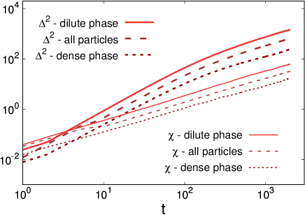
Figure 7: (Color online.) Active system within MIPS. Pe = 50 and $\phi=0.5$. Time-delay dependence in log-log scale of the mean square displacement (thick lines) and integrated linear response (thin lines) calculated averaging only over the particles which spent enough time in the gaseous phase (solid), in the cluster phase (dotted) or over all particles in the system (dashed).

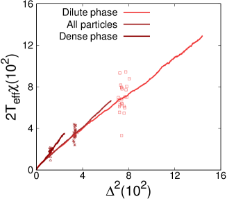
Figure 8: (Color online.) Active system within MIPS. Pe = 50 and $\phi=0.6$. The parametric construction for particles in the dilute and dense phases. The global data are also shown. In all cases the integrated linear susceptibility is multiplied by the global $2T_{\rm eff}$ so as the two quantities vary over the same interval. The data-points are the results for each of the 22 runs performed.

The question is, now, how does the effective temperature depend on the packing fraction, when this one varies from one end to the other end of MIPS at fixed Pe. Plots of $T_{\rm eff}(\phi)/T_{\rm eff}(0)$ as a function of time delay for four representative values of the packing fraction going from the lower to the higher are displayed in Fig. 9. For all $\phi$, after a transient of roughly $400$, the asymptotic plateau is at different heights for the dilute and dense phases and, consequently, the global value is in between these two. The data also demonstrate that the effective temperature of the whole system progressively changes from being equal to the one of the dilute phase, at low $\phi$, to reaching the one of the dense phase, at high $\phi$. We also see that the value of the effective temperature of each of the two phases does not change much with $\phi$. Clearly, as the fraction of particles belonging to the dilute phase diminishes, the corresponding $T_{\rm eff}$ data becomes noisier.

(a)                                     (b)                         

 

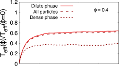
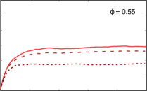
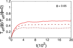
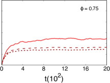
(c)                                     (d)                         

Figure 9: (Color online.) Active system across MIPS. The effective temperatures of the dilute and dense subsystems (continuous and dotted lines, respectively), together with the one of the full system (dashed lines) at Pe = 50, all normalized by the single particle value at this Pe. The densities considered are $\phi=0.4$ (a), $\phi=0.55$ (b), $\phi=0.65$ (c) and $\phi=0.75$ (d). Data are averaged over 60 independent runs.

Figure 10 summarizes the picture that emerges. The figure presents the global packing fraction dependence of the effective temperatures of particles belonging to the dense and dilute phases in between the two measuring times. The data are presented normalized by the effective temperature of the single particle with the same value of Pe. At the limits of co-existence the effective temperature of the majority phase joins the one of the whole system. The limiting values $\phi_{<}$ and $\phi_{>}$ thus measured (showed with vertical dashed lines in the figure) coincide with the ones measured more conventionally to delimit the MIPS region of the phase diagram (within numerical accuracy) Digregorio et al. (2018). We notice that the effective temperature of the two phases are approximately constant within MIPS, with deviations appearing at the border which are due, presumably, to the fact that the fraction of system occupied by one of the phases approaches zero. The value of the effective temperature of the whole system, instead, changes and this is because the portion of particles belonging to each phase vary going from a purely dilute to a purely dense limit as $\phi$ increases.

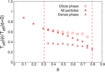
Figure 10: (Color online.) Active system across MIPS. The global packing fraction dependence of the effective temperature of the dense (triangles) and dilute (squares) regions, compared to the one of the whole system (stars), at Pe = 50. The dotted vertical lines indicate the limits of MIPS for this Pe value, $\phi_{<}$ and $\phi_{>}$.

IV Fluctuations

In this Section we aim to complement the study of globally averaged diffusive and response properties with the one of their fluctuations. Having access to the individual square displacement and the product of the position and time-integrated noise, which once averaged over the latter yields the susceptibility, allows us to study their statistical properties. Also, it permits us to correlate them with the local structure of the system.

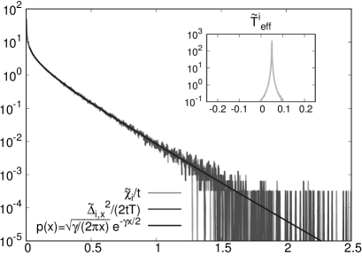
Figure 11: (Color online.) Fluctuations in the passive and very dilute system, Pe = 0 and $\phi=0.001$, with $t_{w}=0$ and $x(0)=0$. Main plot: probability distribution functions of the individual square displacement, $\tilde{\Delta}_{i,x}^{2}$, see Eq. (22), normalized by $2tT$ with $T$ the temperature of the bath, and time integral of the product of position and noise, $\tilde{\chi}_{i}$ defined in Eq. (23), normalized by $t$. The measurements were done using a time-delay $t\simeq 5\times 10^{4}$. The solid black line is the analytical prediction for the single passive particle distribution, Eq. (27). The average values of $\tilde{\chi}_{i}/t$ and $\tilde{\Delta}_{i,x}^{2}/(2tT)$ equal $1/\gamma=0.1$ within numerical accuracy, as consistently predicted by Eq. (27). Inset: probability distribution of the effective temperature defined in Eq. (24). With the choice $t_{w}=0$ and for $\phi=0$ the distribution should collapse on a delta function centered on the bath temperature ($T=0.05$ in simulation units), since the response and the squared displacement divided by $2T$ become just identical in this particular case.

As noted in Corberi and Cugliandolo (2012), for a system with dynamics ruled by a Langevin equation, relations of the type in Eq. (20) give two fluctuating fields, $\partial x_{i}^{\lambda}(t)/\partial\lambda|_{\lambda=0}$ (the superscript $\lambda$ indicates that the dynamics is perturbed) and ${\int_{0}^{t}dt^{\prime}x_{i}(t)\xi_{i}(t^{\prime})/\sqrt{2\gamma T}}$ (whose noise averages yield the linear response function) as the candidates to define the fluctuating part. However, even though these objects have the same thermal average, they may have different fluctuation spectra and higher order correlations. The second field exhibits interesting properties in the case of aging spin-glasses and ferromagnetic systems Castillo et al. (2002, 2003); Chamon and Cugliandolo (2007). The fact that Eq. (20) holds also in a systems of active Brownian particles suggests to associate the fluctuations of the response function to this same field. The Malliavin method allows us to use the same noise realisation and the same stochastic trajectory to compute both this fluctuating quantity and the displacement fluctuations.

The strategy we will follow in the rest of this Section is the following. First of all, we select a time-delay $t-t_{w}$ such that the global (and noise-averaged) mean square displacement is (approximately) diffusive and the (also global and noise averaged) integrated linear response is linear in time. We then analyze the statistics of the single particle displacement, the van Hove function, the ones of the single particle square displacement

$$\tilde{\Delta}_{i,x}^{2}(t,t_{w})\equiv[x_{i}(t)-x_{i}(t_{w})]^{2}\;,$$ (22)

and the ones of integrated linear response

$$\tilde{\chi}_{i}(t,t_{w})=\frac{1}{\sqrt{2\gamma T}}\int_{t_{w}}^{t}dt^{\prime}\,x_{i}(t)\xi_{i}(t^{\prime})\;.$$ (23)

To avoid using wide horizontal intervals in the plots, and to compare the two fluctuating quantities in the manner imposed by the FDT, we divide $\tilde{\Delta}_{i,x}^{2}(t,t_{w})$ by $2(t-t_{w})T$ and $\tilde{\chi}_{i}(t,t_{w})$ by $t-t_{w}$. The reason why in this section we let $t_{w}$ be greater than zero will become clear soon. We also define a local effective temperature as

$$\tilde{T}_{\rm eff}^{i}(t,t_{w})\equiv\frac{\tilde{\Delta}_{i,x}^{2}(t,t_{w})}{2\left[\int_{t_{w}}^{t}x_{i}(t)\xi_{i}(t^{\prime})dt^{\prime}/\sqrt{2\gamma T}\right]}\;.$$ (24)

Note that the average over $i$ of the latter is not necessarily equal to the global effective temperature. We also use a normal representation in which we subtract the global averages and divide by the standard deviation.

IV.1 A single passive particle

For a single passive Brownian particle in the over-damped regime, the explicit solution of the Langevin equation implies

$$\tilde{\Delta}(t,t_{w})=x(t)-x(t_{w})=\frac{\sqrt{2\gamma T}}{\gamma}\int_{t_{w}}^{t}\xi(s)\;ds\;.$$ (25)

Consequently, the fluctuating time-integrated linear response function can also be written as

$$\tilde{\chi}(t,t_{w})=\frac{1}{2T}\,x(t)\,[x(t)-x(t_{w})]\;,$$ (26)

that is to say, the product of two Gaussian random variables. For the particular choice $t_{w}=0$ and $x(t_{w}=0)=0$, the time-integrated response function is just proportional to the square of $x(t)$, and $\tilde{\chi}(t,0)$ becomes identical to $\tilde{\Delta}_{i,x}^{2}(t,0)/2T$. The fluctuating linear response (divided by $t$) and the square displacement (divided by $2tT$) are equally distributed according to

$$p(x)=\sqrt{\frac{\gamma}{2\pi x}}\ e^{-\gamma x/2}$$ (27)

for $x\geq 0$. This is in agreement with one of the results shown in Corberi and Cugliandolo (2012) and it could also be derived exploiting the symmetries exhibited by the joint probability distribution functions derived in that paper. Notice that setting $t_{w}=0$, the effective temperature becomes identically equal to the temperature of the bath and therefore its probability distribution is just a delta function centered at $T$. Figure 11 shows that in the dilute passive case the distribution of the effective temperature resembles a delta function (inset; note that the small distribution spread is solely due to inter particle interactions, and disappears when considering a single particle), while the pdfs of the response and the squared displacement are numerically equal and follow very closely Eq. (27) for the single over-damped Brownian passive particle.

The mean squared displacement is independent on the particular value of $t_{w}$ since it is a function of the time delay alone. It is clear from the same definition of the squared displacement, Eq. (22), that also its distribution function depends only on $\Delta t=t-t_{w}$ and not on its average.

These considerations are no longer valid when we consider the distribution of the response function. When setting $t_{w}\neq 0$, the fluctuating part of the response becomes the product of two correlated Gaussian variables with correlation coefficient strictly less than one, see Eq. (26). Since the joint probability distribution function of each of these two variables is also Gaussian, it is possible to evaluate exactly the pdf of their product; it reads

$$p_{\left.\frac{\tilde{\chi}(t,t_{w})}{t-t_{w}}\right|_{t_{w}\neq 0}}(x)$$

$$\qquad=\frac{\gamma(t-t_{w})\exp\left[\frac{\gamma(t-t_{w})x}{t_{w}}\right]}{\pi\sqrt{t(t-t_{w})-(t-t_{w})^{2}}}$$

$$\qquad\qquad\times\;K_{0}\left(\sqrt{\frac{\gamma^{2}(t-t_{w})t}{t_{w}^{2}}}\,|x|\right)\;,$$ (28)

where $K_{0}$ is the modified Bessel function of the second kind of order zero. In the limit $t\gg t_{w}$ and $x>0$ one recovers the form in Eq. (27). The distribution of the response does depend explicitly on the waiting time. Only if $t_{w}=0$ the distribution exhibits a single branch for positive values, since in this particular case we are evaluating the pdf of the product of two perfectly correlated Gaussian random variables, see Fig. 11. As soon as $t_{w}$ becomes greater than zero, the pdf develops a negative branch. Notice that this particular feature does not affect the average of the distribution which equals $1/\gamma$ for every value of the waiting time.

We checked this calculation numerically by comparing the distributions of the time-integrated response in a very dilute ($\phi=0.001$) system of passive Brownian particles and different waiting times with the analytical predictions, see Fig. 12.

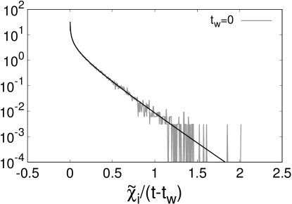
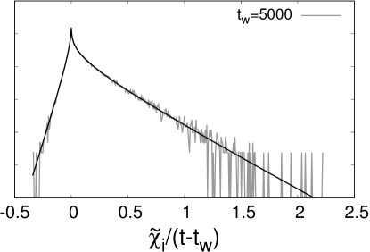
Figure 12: Probability distribution function of $\tilde{\chi}(t,t_{w})/(t-t_{w})$ at Pe = 0 and $\phi=0.001$ evaluated at fixed $\Delta t=5\times 10^{3}$ and waiting times given in the caption. Black lines: analytical predictions in Eq. (27) for $t_{w}=0$ and Eq. (28) for $t_{w}\neq 0$.

We want to underline that the distributions of $\tilde{\chi}_{i}$ for different values of the waiting time do not collapse on top of each other even when plotted in normal form. In spite of this, as the waiting time grows, the dependence on $t_{w}$ becomes less evident, see Fig. 13. We will exploit it when studying the active particle and interacting finite density problems.

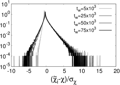
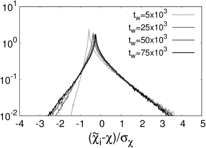
(a)                                     (b)

Figure 13: (a) Probability distribution function of the time-integrated linear response in normal form at Pe = 0 and $\phi=0.001$ for $\Delta t=5\times 10^{3}$ and different values of the waiting time given in the key. (b) Enlargement of the distribution peaks. For increasing $t_{w}$ the distributions tend to collapse on the same curve.

The single particle effective temperature, Eq. (24), can be simplified in the same way by using the explicit solution of the Langevin equation

$$\tilde{T}_{\rm eff}(t,t_{w})=T\;\frac{x(t)-x(t_{w})}{x(t)}\;.$$ (29)

Therefore, for a single passive particle, the effective temperature is given by the ratio of two correlated Gaussian variables with known joint probability distribution. A quite long but straightforward calculation leads to

$$p_{\tilde{T}_{\rm eff}(t,t_{w})}(x)=\frac{1}{\pi}\frac{A}{A^{2}+(x-x_{0})^{2}}$$ (30)

with

$$\begin{array}[]{rcl}A&=&T\sqrt{(t-t_{w})t_{w}/t^{2}}\;,\vspace{0.2cm}\\ x_{0}&=&T(t-t_{w})/t\;,\end{array}$$ (33)

that is to say, a Cauchy distribution centered at the maximum $x=x_{0}$ with height $1/(\pi A)$. For $t\gg t_{w}$, $A\to 0$, $x_{0}\to T$, and the form approaches $\delta(x-T)$. This last limit also applies in the case $t_{w}=0$ and $t\neq 0$.

Notice that, since neither the mean value of the squared displacement nor the average of the response function depend on the choice of $t_{w}$, the value of the effective temperature, $T_{\rm eff}$, is not affected by its particular choice. Instead, the distribution of $\tilde{T}_{\rm eff}^{i}(t,t_{w})$ does depend on the waiting time when $t$ is not much larger than $t_{w}$.

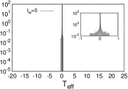
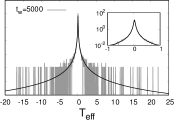
Figure 14: Probability distribution function of $\tilde{T}_{\rm eff}^{i}(t,t_{w})$ at Pe = 0 and $\phi=0.001$ evaluated at fixed $\Delta t=5\times 10^{3}$ and waiting times given in the keys. Black lines: analytical predictions Eq. (30) for $t_{w}\neq 0$ and $\delta(x-T)$ for $t_{w}=0$. In the inset, zooms over the peaks centered at 0.

We evaluated numerically the distributions of the single particle effective temperature with different waiting times, again in a very dilute system of passive particles, and we compared the results with the analytical prediction in Eqs. (30)-(33), see Fig. 14, finding very good agreement between numerical and analytic results.

IV.2 A single active particle

For a single active particle in the overdamped limit, the distribution of the displacement in a fixed direction is still Gaussian both at short and long times with a variance determined by the temperature of the bath in the first case and by the effective temperature in the latter one Sevilla and Sandoval (2015). Accordingly, the distribution of the squared displacement (divided by $2T_{\rm eff}$) is given by Eq. (27). For the same reason, at long time, the response function is the product of two Gaussian variables: the variance of the first one (the position of the particle) depends on the effective temperature and the whole time interval $t$, while the variance of the second one (the integral of the thermal noise) depends on the temperature of the heat bath and the measuring time $t-t_{w}$. Therefore, the probability distribution function of the response in the active case is the analogue of Eq. (28) after a proper mapping of the coefficients:

$$p_{\frac{\tilde{\chi}(t,t_{w})}{t-t_{w}}}(x)=\frac{\sqrt{T}}{\pi}\frac{\gamma(t-t_{w})}{\sqrt{T_{\text{eff}}\,t(t-t_{w})-T\,(t-t_{w})^{2}}}$$

$$\qquad\times\;\exp\left[\frac{T\,\gamma\,(t-t_{w})x}{T_{\text{eff}}\,t-T\,(t-t_{w})}\right]$$

$$\qquad\times\;K_{0}\left(\sqrt{\frac{T_{\text{eff}}\,T\,\gamma^{2}\,t(t-t_{w})}{\left[T_{\text{eff}}\,t-T\,(t-t_{w})\right]^{2}}}\,|x|\right)\;.$$ (34)

Notice that, since $T_{\text{eff}}>T$, the determinant of the correlation matrix of the two Gaussians does not vanish even if $t_{w}=0$. Thus, in the active case a negative branch is always present. Indeed, since the active particle is not moving solely under the influence of the thermal noise, even when the measuring time coincides with the whole time interval there is the possibility that the displacement of the particle is opposite to the integrated noise. The weight of this negative branch is enhanced for higher activity and we do expect that the presence of interparticles forces would produce similar effects.

The evaluation of the probability distribution function of the effective temperature in the active case is not straightforward since the simplification we performed in the passive case exploits the explicit solution of the equation of motion and it is no longer valid. In spite of that, if we restrict the analysis to the case $t_{w}=0$ with $x(0)=0$ (since only the shape of the distribution is affected by the particular choice of the waiting time, while the average is not), it is possible to simplify the expression for the effective temperature,

$$\tilde{T}_{\text{eff}}(t,0)=\sqrt{\frac{T\gamma}{2}}\frac{x(t)}{\int_{0}^{t}dt^{\prime}\,\xi(t^{\prime})}\;.$$ (35)

and its statistics are given by another Cauchy distribution with coefficients

$$\begin{array}[]{rcl}A&=&\dfrac{T}{T_{\rm eff}}\sqrt{T(T_{\rm eff}-T)}\;,\vspace{0.2cm}\\ x_{0}&=&T^{2}/T_{\rm eff}\;,\end{array}$$ (38)

that reduce to the values in Eq. (33) in the passive limit $T_{\rm eff}=T$.

 

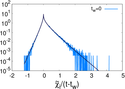
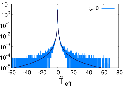
(a)                                     (b)

Figure 15: Probability distributions of (a) the time-integrated linear response and (b) the effective temperature, for $t_{w}=0$, in a very dilute active system approaching the single particle limit. Pe = 5 and $\phi=0.001$. Solid lines: analytical predictions given by Eq. (34) in (a) and Eq. (38) in (b).

Notably, while in the passive case (if $t_{w}=0$) the effective temperature is identically equal to the temperature of the heat bath, in the active case its distribution is not simply a delta function centered on its global value. In Fig. 15, we compare the numerical distribution of the response and the effective temperature for a single active particle with the analytical predictions in Eq. (34) and Eq. (38) and once again the comparison is very favorable.

IV.3 Homogeneous phase

Having clarified the behavior of the fluctuations in the single particle case, we now turn to the problem of a dense homogeneous passive and active system.

In equilibrium, the averaged square displacement and response function exhibit an explicit dependence on the density of the system. In particular, these averages diminish when the density is increased, though in such a way that their ratio remains independent of the packing fraction and always yields the same effective temperature, equal to the temperature of the heat bath.

When considering the out of equilibrium active case, we found a dependence of the effective temperature on the global density of the system. This effect is due to two combined reasons: the mean value of the squared displacement decreases more than it does in the passive case with $\phi$, while the average of the response function also does but in a less pronounced way.

We expect to retrieve similar features when studying the fluctuations of the displacement and the response in the homogeneous region of the phase diagram. Let us see now if this is indeed so.

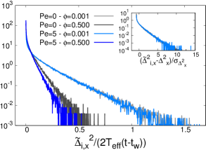
Figure 16: Main plot: distribution of the individual square displacement divided by $2T(t-t_{w})$ in the passive case (Pe = 0) and by $2T_{\rm eff}(t-t_{w})$ in the active one (Pe = 5). Comparison between the behavior in the very dilute ($\phi=0.001$) and in a dense case ($\phi=0.500$). Inset: probability distribution functions of the individual square displacement, $\tilde{\Delta}_{i,x}^{2}$, in normal form. All four curves collapse on top of each other. The waiting time for the measurement is $t_{w}=10^{5}$ and the delay time $\Delta t\equiv t-t_{w}=5\times 10^{3}$.

IV.3.1 The displacement

The individual displacements are typically enhanced by the activity and their distribution develops a longer tail. On the contrary, increasing the packing fraction the dynamics get more sluggish and the individual displacements are reduced making their distribution narrower.

Still, under both kinds of changes, the displacement distributions preserve the functional form in Eq. (27). We will make the working hypothesis that for weak activity and not too high density, $x(t)-x(t_{w})$ remains Gaussian distributed (note that at sufficiently high density there could be deviations from this simple statistics Phillies (2015)). Therefore, the distribution of the squared displacement is still given by the one of the product of two perfectly correlated Gaussian variables.

We confirm these claims in Fig. 16, where we analyze the distribution of $\tilde{\Delta}_{i,x}^{2}/(2T(t-t_{w}))$ and $\tilde{\Delta}_{i,x}^{2}/(2T_{\rm eff}(t-t_{w}))$, with $T_{\rm eff}$ the single particle effective temperature, in the passive and active cases, respectively. In the very dilute limit, the distributions collapse almost perfectly on top of each other, according to Eq. (27). When the density is increased they keep the same functional form but their tails scale differently. The drop in the active dense case is more pronounced than in the passive dense one (compare the dark blue and gray curves in Fig. 16), although notice that without dividing by $T$ and $T_{\rm eff}$ the displacements of the active particles are much larger than the passive ones, as $T_{\rm eff}$ is proportional to Pe².

In the inset of Fig. 16, we study this same observable in its normal form. Although the displacements are enhanced by the activity, the distribution of $(\tilde{\Delta}_{i,x}^{2}-\Delta_{x}^{2})/\sigma_{\Delta_{x}^{2}}$, is independent of both the active force and the global packing fraction, as the various distributions of the individual displacements collapse on each other.

IV.3.2 The linear response

First, we notice that turning on the activity and increasing the density produce similar effects, in the sense that both of these changes reduce the correlation between the position of each particle at time $t$ and the integral of the noise acting on it between $t_{w}$ and $t$. In fact, the correlation is maximal when the latter represents the only force exerted on the particle.

The shape of the probability distribution function of $\tilde{\chi}_{i}$ remains similar to the reference case (Pe = 0 and $\phi=0.001$): it preserves a sharp peak at zero and two wings that depart from the peak. These features are shown in Fig. 17. The skewness of the susceptibility probability distribution function is also clear in all the plots that we present in this part of the paper.

(a)                                        

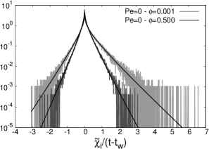
(b)                                        

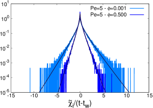
Figure 17: Fluctuations of the time integral of the product of position and noise, $\tilde{\chi}_{i}$, divided by $t-t_{w}$, see Eq. (21). Passive (Pe = 0, (a)) and active (Pe = 5, (b)) systems: comparison between the behavior in the dilute limit ($\phi=0.001$) and in the dense homogeneous systems ($\phi=0.500$). The probability distribution functions are fitted using Eq. (40) with $t_{w}=10^{5}$ and $b=2T\,(t-t_{w})/\gamma$ in all cases. In the dilute limit $c=2T\,(t-t_{w})/\gamma$ while $a$ is obtained from the Gaussian distribution of the displacement (not shown) in the four cases. Fitted parameters: $a=1050$ (Pe = 0, $\phi=0.001$), $a=359.4$ and $c=13.7$ (Pe = 0, $\phi=0.500$); $a=5425$ (Pe = 5, $\phi=0.001$), $a=1310$ and $c=19.6$ (Pe = 5, $\phi=0.500$).

As in the single particle case, we found an explicit dependence on the waiting time. However, the dependency is weaker due to, at fixed $t_{w}$, the presence of the active force (in the active dilute case), or the presence of the inter-particle forces (in the dense passive case) which reduce the correlations between the position and the integral of the noise. Therefore the value of the waiting time over which the distributions (in normal form) collapse is reached earlier.

In order to evaluate the probability distribution of the linear response, for each particle we rewrite it as

$$\frac{\tilde{\chi}_{i}(t,t_{w})}{t-t_{w}}=\frac{X\cdot Y}{2T(t-t_{w})}\;,$$ (39)

with $X=x_{i}(t)$ and $Y=\sqrt{2T/\gamma}\int_{t_{w}}^{t}\xi_{i}(t^{\prime})\,dt^{\prime}$. We consider $t_{w}\neq 0$ and we find

$$p_{\frac{\tilde{\chi}_{i}(t,t_{w})}{t-t_{w}}}(x)$$

$$\qquad=\frac{2T(t-t_{w})}{\pi\sqrt{|ab-c^{2}|}}\exp\left[2T(t-t_{w})\frac{c}{ab-c^{2}}\,x\right]$$

$$\qquad\qquad\times\;K_{0}\left(2T(t-t_{w})\frac{\sqrt{ab}}{ab-c^{2}}\,|x|\right)\;,$$ (40)

with $a=\braket{X^{2}}$, $b=\braket{Y^{2}}$ and $c=\braket{X\cdot Y}$. In the single particle case discussed in the previous subsection $a=2T_{\text{eff}}\,t/\gamma$, $b=c=2T\,(t-t_{w})/\gamma$. When the density is increased, we notice that the functional form of the distributions remains unchanged, while the value of the coefficients may depend on the density and the activity. In particular $b$, being simply the variance of the noise, is unaffected by these changes. We have already noticed that $a$ (which is the mean squared displacement) is reduced in the active case with the increase of $\phi$ more than it is in the equilibrium limit. This effect would not explain the reason why the response function behaves in the opposite way. We expect that, in the active case, $c$ which is proportional to the average of $\tilde{\chi}$ and yields the linear response, be slightly less sensitive to the increase of the packing fraction. Therefore, when $\phi$ is increased the correlation between the position of the particle and the integral of the noise diminishes in the active case slightly less than it does in the passive case.

We support these claims with our numerical results. We chose a long waiting time, $t_{w}=10^{5}$, and we measured the linear response in systems with Pe = 0, 5 and $\phi=0.001,\,0.500$. In Fig. 17, we compare the numerical data collected in these four cases with the functional form in Eq. (40), using $c$ as the only fitting parameter (we kept $b=2T\,(t-t_{w})/\gamma$ and we used for $a$ the value determined by the distribution of the position).

From the examples in Fig. 17, we can clearly see that the shape of the linear response distribution is unchanged when the density or the activity are increased with respect to the single Brownian particle case. The fitted parameters are written in the caption.

IV.3.3 The effective temperature

In the passive limit, the combination of the parameter effects on the displacements and linear response fluctuations always lead to the same global effective temperature which is found to coincide with the temperature of the bath, in agreement with the results in Fig. 5. In the active case the global effective temperature is found to be always higher than the bath temperature, but lower than the one for the single active particle, see Fig. 3.

In this subsection, we briefly explore how the distribution of the single particle effective temperature, defined in Eq. (24), changes when $\phi$ is increased. As we noticed when we evaluated the probability distribution function of the effective temperature of a single active particle, the simplification we performed for a passive Brownian particle is no longer valid when other forces come into play. These considerations hold when we turn on the activity as well as when the particles interact among themselves. However, if we choose $t_{w}=0$, we are allowed to simplify the expression of the single particle effective temperature:

$$\tilde{T}_{{\text{eff}}_{i}}(t,0)=\sqrt{\frac{T\gamma}{2}}\frac{x_{i}(t)}{\int_{0}^{t}dt^{\prime}\,\xi_{i}(t^{\prime})}\equiv T\,\frac{X}{Y}\;.$$ (41)

Under this particular condition, $\tilde{T}_{{\text{eff}}_{i}}$ is again the ratio of two Gaussian variables. With the convention $a=\braket{X^{2}}$, $b=\braket{Y^{2}}$ and $c=\braket{X\cdot Y}$, the probability distribution function of $\tilde{T}_{{\text{eff}}_{i}}$ is again a Cauchy distribution with coefficients:

$$A=T\,\frac{\sqrt{ab-c^{2}}}{b}\;,\qquad\quad x_{0}=T\,\frac{c}{b}\;.$$ (42)

The coefficient $b$, being proportional to the variance of the thermal noise, remains fixed whether the system is passive or active, no matter the density. Therefore we will keep $b=2Tt/\gamma$. Besides, $a$ can be estimated from the variance of the displacement of the particle. Again, $c$ is the only fitting parameter. We expect that the peak of the distribution, i.e. $x_{0}$, be unaffected by the presence of the active force in the dilute limit (since the activity does not change the correlation between the position of the particle and the integral of the noise acting on it), while it should be affected by the interparticle forces. Since the covariance diminishes, the peak should be shifted toward zero. Notice that for a single Brownian particle, $a=b=c$ at $t_{w}=0$, $A\to 0$ and the distribution reduces to a delta function centered on $T$ as previously described.

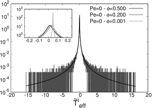
(a)

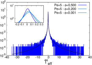
(b)

Figure 18: Fluctuations of the single particle effective temperature $\tilde{T}_{{\rm eff}_{i}}$, see Eq. (24). The distributions in the main plots are fitted using a Cauchy distribution with coefficients given by Eq. (42), with $b=2Tt/\gamma$, $a$ obtained from the Gaussian distribution of the displacement (not shown) and $c$ a fitting parameter. All the distributions are evaluated at $t_{w}=0$. Fitting parameters: $c=17.1$ (Pe = 0, $\phi=0.5$) and $c=19.15$ (Pe = 5, $\phi=0.5$). In the insets, enlargements of the peaks of the distributions for different values of the density are displayed.

In Fig. 18, we show how the statistics of the single particle effective temperature, defined in Eq. (24), changes when the density is increased from the very dilute limit both in the equilibrium (panel (a)) and in the active non equilibrium case (panel (b)). As anticipated above, the position of the peak is not affected by the active force and it remains around the temperature of the heat bath in the dilute limit (in simulation units $T=0.05$). When the density is increased the peak is shifted towards zero in both cases. On the other hand, in the equilibrium case the density increase does not change appreciably the width of the distribution, while in the active one increasing the density causes a shrinking of the probability distribution function. This feature is reflected in a decrease of the coefficient $A$ in the latter case. We note that the distributions for different $\phi$ and Pe collapse on each other when put in normal form (apart from the $\phi=0.001$, Pe = 0 one, which is close to a delta function.

As a concluding remark, we notice that if we consider $t_{w}\neq 0$, the distribution of the effective temperature in the dense passive and active cases cannot be fitted with a Cauchy distribution.

IV.4 Heterogeneous phases

In the heterogeneous phases, especially in MIPS, we need to consider long time delays (of the order $\Delta t=5\times 10^{3}$) to ensure that a large number of particles reach the diffusive regime. The problem with this choice is that the bimodal structure of the pdf of the time-delayed averaged hexatic parameter is smoothed and a lot of particles can not be considered to belong to one and only one phase during the full long time interval. Although this does not affect sensibly the time average, it can interfere, as we will see, in the distribution form. We therefore adopted a criterium with two different thresholds to separate the particles into those belonging to the dilute and dense phases: the particles contributing to the dilute distributions are the ones with mean hexatic order parameter on the left side of the first peak, while the ones contributing to the dense distributions are the ones with mean hexatic order parameter on the right side of the second peak, see panel (c) of Fig. 4 or panel (b) of Fig. 6. We then leave out from the distributions the particles with mean hexatic order parameter in between the two thresholds. For similar reasons, in this section we will always consider $t_{w}=0$. Since we can not access very long times keeping a satisfactory particles distinction, we prefer to maximize the measuring time $\Delta t=t-t_{w}$ to the detriment of the waiting time.

We now study systems in their co-existence regions, be them close to Pe = 0 or at high Pe, with a packing fraction roughly in the middle of the MIPS region of the phase diagram. The aim is to compare the fluctuations of the individual displacement and response in the two coexisting phases to better understand the origin of the different effective temperatures at the global level (after averaging over all the particles belonging to each phase).

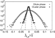
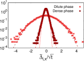
(a)                                     (b)

Figure 19: Fluctuations in the passive system in the co-existence region of the phase diagram (panel (a) Pe = 0 and $\phi=0.71$) and in the active system in the MIPS region of the phase diagram (panel (b) Pe = 50 and $\phi=0.6$). Probability distribution functions of the individual displacements normalized with respect to the squared root of the elapsed time ($t=5\times 10^{3}$) in the fluid and in the dense phase. The distribution in the fluid phase is fitted using a Gaussian function, while in the cluster phase the tails are fitted with exponential decays.

IV.4.1 Passive case

In Fig. 19 (a), we show the pdf of the single particle displacement, $\tilde{\Delta}_{i,x}$, in the coexistence region. On the one hand, the data for the particles belonging to the fluid phase are almost perfectly well fitted by a Gaussian function. Instead, the data for particles belonging to the denser cluster phase are not only narrower but also different. While the central part is well described by a Gaussian distribution, the tails strongly deviate from this behavior and decay exponentially (with slight deviations possibly due to the presence of some residual particles with mixed dynamics). If we look at the distribution of the particle displacements in the homogeneous hexatic phase (Pe = 0, $\phi=0.726$, not shown) this small effect disappears and the tails are perfectly described by an exponential distribution. (Exponential tails are also observed, for example, in complex liquids, see Phillies (2015) and references therein.)

Figure 20: Fluctuations in the passive system, Pe = 0 and $\phi=0.71$, in the co-existence region of the phase diagram (same data as in Fig. 19, panel (a)). Probability distribution functions of the individual square displacement, $\tilde{\Delta}_{i,x}^{2}$, in normal form.

The changes in the statistics of $\tilde{\Delta}_{i,x}$ are quite naturally reflected in the distribution of the squared displacement that we show in Fig. 20 for the same parameters. In normal form, the distribution of the particles in the dilute component resembles strongly the one in the homogeneous liquid state, with the pdf of the individual displacements falling on top of the single particle distribution. On the other hand, the exponential tails in the distribution of the displacement of the particles in the dense component gives rise to a wider exponential tail in the pdf of the square displacement which does not follow the trend of the reference case.

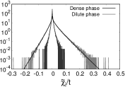
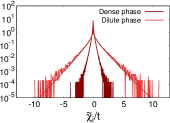
(a)                                     (b)

Figure 21: Fluctuations in the passive system, Pe = 0 and $\phi=0.71$, in the co-existence region of the phase diagram (panel (a)) and in the active system, Pe = 50 and $\phi=0.6$, in the MIPS region (panel (b)). Probability distribution functions of the response $\tilde{\chi}_{i}$ defined in Eq. (21) divided by the measuring time $t=5\times 10^{3}$ in the dilute and dense phases. In the dilute case, the pdf is fitted using Eq. (40) with $t_{w}=0$ and $b=2T\,t/\gamma$, while $a$ is obtained from the Gaussian distribution of the displacement. Fitted parameter: $c=3.3059$ (passive case) and $c=17.97$ (active case). The shape of the distribution in the dense phase is different and it cannot be fitted using similar arguments.

The effects of the changes in the distribution of the particle displacements are felt also by the fluctuations of the response functions. In Fig. 21 (a), we show the fluctuations of the single particle response $\tilde{\chi}_{i}$ defined in Eq. (21), divided by the measuring time, in the co-existing dilute liquid and dense hexatic phases. The pdf for the particles in the dilute phase is similar to what we found in the homogeneous fluid phase. Indeed, the distribution can be fitted using Eq. (40) with $t_{w}=0$ and the procedure explained above. Importantly, even though the densities of the two phases are very close, the shape of the distribution in the hexatic phase is different: the pdf is tighter, its skewness is reduced, and it cannot be fitted using Eq. (40), mainly because of deviations in the tails.

In Fig. 22, we show the distribution of the single particle effective temperature defined in Eq. (24) evaluated in the two phases separately. The distribution of the dilute phase appears broader, as expected. From the enlargement shown in the inset, it is clear that the peak of the distribution of the dense phase is sharper than the one of the dilute phase and it is shifted around zero.

Following the same strategy that we used in the study of the homogeneous system, we fitted the pdf of the dilute phase using a Cauchy distribution, Eq. (30). The fitted parameter is written in the caption. Notice that, naturally enough, it is compatible with the fit performed for the response function. We do not expect that the distribution in the denser hexatic phase preserves a similar shape. In spite of that, we find that the central part of the pdf can still be described by a Cauchy distribution with violations in the tails. It is clear the particles with Gaussian distruibuted displacement contribute to the peak, while those which contribute to the exponential tail of the displacement pdf also contribute to the tails of the pdf of the effective temperature.

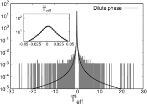
(a)

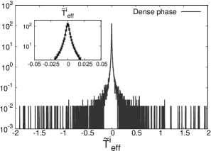
(b)

Figure 22: Fluctuations of the single particle effective temperature $\tilde{T}_{{\rm eff}_{i}}$, see Eq. (24), in the dilute (a) and in the dense phase (b) coexisting at Pe = 0, $\phi=0.71$. The distributions are fitted using a Cauchy distribution with coefficients given by Eq. (42), with $b=2Tt/\gamma$, $a$ obtained from the Gaussian distribution of the displacement and $c$ a free parameter, taking values $c=3.38$ (dilute phase) and $c=0.11$ (dense phase). All the distributions are evaluated at $t_{w}=0$. In the insets, enlargements of the peaks for different values of the density.

IV.4.2 MIPS

We now turn to the study of the fluctuations under strong activity, in the MIPS region of the phase diagram.

In Fig. 19 (b), we show the distribution of $\Delta_{i,x}$ in the dilute and dense phases. The curves are similar to the ones in the equilibrium heterogeneous phase (panel (a) of the same figure): Gaussian for particles in the dilute component while, in the denser component, only the central part of the distribution is normal and the tails decay exponentially. In spite of these similarities, we also notice some differences. Firstly, there are some deviations from the Gaussian behavior in the tails of the distribution of the dilute component, possibly due to a partial mixture between the phases. Secondly, even considering the same measuring time ($t=5\times 10^{3}$), the exponential tails are much more evident in the active than in the passive case.

The Gaussian character of the displacements in the dilute phase leads to the collapse of the distribution of the squared displacement $\tilde{\Delta}^{2}_{i,x}$ on top of the reference single particle one, when plotted in normal form (not shown), while in the dense phase the distribution develops a longer exponential tail, similarly to the passive case.

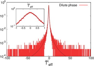
(a)

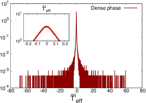
(b)

Figure 23: Fluctuations of the single particle effective temperature $\tilde{T}_{{\rm eff}_{i}}$, Eq. (24), in the dilute (a) and dense phase (b) coexisting at Pe = 50 and $\phi=0.6$. The distributions are fitted using a Cauchy distribution with coefficients given by Eq. (42), with $b=2Tt/\gamma$, $a$ obtained from the Gaussian distribution of the displacement and $c$ a fitting parameter. All the distribution are evaluated at $t_{w}=0$. Fitted parameters: $c=14.52$ (dilute phase) and $c=2.09$ (dense phase). In the insets, enlargements of the peaks of the distributions for different values of the density.

The fluctuations of the individual linear response, see Fig. 21 (b), also show differences when the particles belong to the dilute and dense phase. While the distribution of the former is well fitted using Eq. (40) and the strategy adopted before, see the caption for the actual values of the parameters, for the latter a similar fit could be performed only in the central part of the distribution, with deviations in the tails. Firstly, notice that, while in the passive case the two phases coexist with very similar densities, in the MIPS region the significant difference in the densities of the phases causes the branches of the distributions to depart from the peak with very different slopes. Secondly, the skewness of the distributions of the individual response tends to disappear also in the dilute phase.

Before concluding the study of the fluctuations, we look at the behavior of the distribution of the single particle effective temperature. The shape of the distributions of $\tilde{T}_{{\rm eff}_{i}}$ in the MIPS region, shown in Fig. 23, resembles the one found in the passive limit (see Fig. 22). The distribution evaluated in the dilute phase is broader than the distribution of the temperatures in the dense phase and, while in the dilute phase the pdf follows a Cauchy distribution, Eq. (30), in the dense phase this holds only for the central part of the pdf, where the particles with Gaussian displacements are found.

IV.5 Summary

The detailed analysis of fluctuations that we presented in the Section can be summarized as follows.

In the homogenous active phase at low density, as in the dilute phase in MIPS, we found:

• Gaussian distributions of the displacement $x_{i}(t)-x_{i}(t_{w})$, that lead to the

• exponential (corrected by an algebraic factor) pdf of the square displacements,

• an exponential times a Bessel function for the linear response leading to different exponential decays for both positive and negative branches in the large argument limits,

• and a Cauchy probability for the individual effective temperatures, in the way we defined them.

The origin of the statistics of $\tilde{\Delta}^{2}_{i},\tilde{\chi}_{i},\tilde{T}_{{\rm eff}_{i}}$ is in the fact that the first one is the product of the two same Gaussian variables, the second the product of two different Gaussian variables, and the third one is the ratio between two Gaussian variables. The parameters of these distributions depend on $\gamma$, $t$ and $t_{w}$. Once put in normal form, all these curves collapse on three master curves that are, basically, the ones of the single active particle.

In the heterogeneous active phase close to the passive limit, it is hard to make conclusive measurements as the two phases have very close density and are rather similar. Still, we have been able to see that the fluctuations in the dense phase are different from the ones in the dilute one. This was more clearly seen in the study of fluctuations in the MIPS region, where the fluctuations of particles belonging to the dilute phase behave just as in the homogeneous cases, while the ones in the dense component have different statistics. The latter are characterized by

• A Gaussian central behaviour and exponential tails for the distribution of $x(t)-x(t_{w})$ that

• modify the tails of the distributions of the square displacement, linear response and effective temperature.

• There is no collapse of the data for the dense and dilute phases on a single master curve even when put in normal form.

V Kinetic vs. effective temperatures

In this Section we compare the (time-delayed) effective temperature to the (instantaneous) kinetic temperature notion, that has been widely used in granular matter studies, but also recently in the context of active matter systems. We will first discuss in Subsec. V.1 the effect of the friction coefficient on the effective temperature, and we will perform the proper comparison between the two quantities in Subsec. V.2.

V.1 The effect of the friction coefficient

The single particle effective temperature ${T_{\text{eff}}}$ depends on ${\gamma}$ only during a transient temporal regime, through the mean squared displacement, see Eq. (11), while its asymptotic value does not. We wish to examine whether the effective temperature of the interacting system is also independent of $\gamma$ after a short irrelevant transient.

As a first check, we evaluate the effective temperature in the homogeneous fluid and we change the value of the damping coefficient. In Fig. 24, we show the time-dependence of ${T_{\text{eff}}}$ in a system with ${\text{Pe}=50}$, ${\phi=0.200}$ and ${\gamma=10,\,100}$. The single particle behavior is inherited in the sense that the effective temperature depends on $\gamma$ only during a first regime, while the stationary value is independent of it.

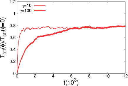
Figure 24: (Color online.) Effective temperature vs time in systems with different damping coefficients. There is a dependence on ${\gamma}$ only in the first regime, while the stationary value is $\gamma$-independent within numerical accuracy. ${\text{Pe}=50}$, ${\phi=0.200}$, ${\gamma=10,\,100}$.

The measurements within MIPS, say for Pe = 50 and $\phi=0.500$, are harder since since for stronger $\gamma$ the time needed to reach the steady state increases. This somehow counterintuitive statement can be understood by looking at the expression for the single particle $\Delta^{2}$, Eq. (11), where the time-scale for the decay of the exponential is $1/D_{\theta}$ with $D_{\theta}=3T/(\gamma\sigma_{\rm d}^{2})$. We find again that the effective temperatures depend on the friction coefficient only during a transient, while they saturate to values that are independent of $\gamma$. This is shown in Fig. 25.

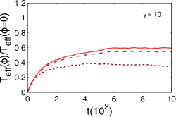
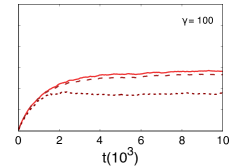
Figure 25: Effective temperature in the MIPS region (Pe=50, $\phi=0.5$) for different damping ratio, $\gamma=10$ (left), $\gamma=100$ (right), of the dilute and dense subsystems, and the one of the full system (continous, dotted and dashed lines, respectively). The measurements with $\gamma=100$ have been performed using $\Delta t=10^{4}$ instead of $\Delta t=10^{3}$.

V.2 The kinetic temperature

The kinetic temperature ${T_{i}^{\text{kin}}}$ is the temperature extracted from the velocity fluctuations. As it is clear from its definition

$$T_{i}^{\text{kin}}\equiv\langle E_{i}^{\text{kin}}(t)\rangle=\frac{1}{2}m\langle v_{i}^{2}(t)\rangle\;,$$ (43)

the kinetic temperature accesses the instantaneous properties of the system, and not the time-delayed ones, with $i$ the particle label. In the inhomogeneous cases we will distinguish the behavior of the particles in the dilute and dense phases. It is quite clear that for Brownian particles one needs to study the stochastic dynamics in the under-damped limit, in which inertia is not neglected, to compute the kinetic energy and from it the kinetic temperature.

The kinetic temperature of a single active particle can be easily calculated by solving the full Langevin equation. After a short transient after which the initial velocity is forgotten, one obtains

$$T_{\text{kin}}=T\left[1+\frac{T}{2\gamma\sigma^{2}}\frac{\text{Pe}^{2}}{\left(\frac{1}{t_{I}}+\frac{1}{t_{A}}\right)}\right]\;,$$ (44)

where ${t_{I}=m/\gamma}$ and ${t_{A}=1/D_{\theta}}$ are the relevant time scales, i.e. the inertial and the active time. In the passive case Pe = 0 and $T_{\text{kin}}=T$ for all the possible values of $t_{I}$. In the active case with $t_{I}\to 0$ one also recovers $T_{\text{kin}}=T$, contrary to what happens with the effective temperature, Eq. (14), that depends explicitly on Pe even in this limit.

In the passive case, we expect the coexisting phases to share the same kinetic temperature which, moreover, should equal the temperature of the thermal bath. In Fig. 26, we show the kinetic temperature of the particles belonging to the hexatic and liquid phases separately: they are equal and, on average, they also coincide with the temperature of the bath.

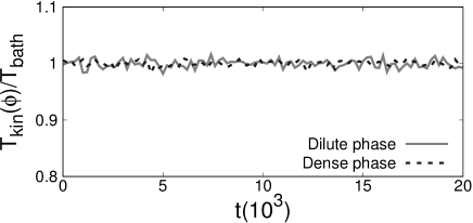
Figure 26: (Color online.) Comparison of the kinetic temperature of the coexisting phases in the passive system. We normalize the kinetic temperature with respect to the bath temperature. ${N=256^{2}}$, ${\text{Pe}=0}$, ${\phi=0.710}$, and ${\gamma=10}$.

We now reconsider the system with ${\text{Pe}=50}$ and ${\phi=0.500}$. We evaluate the kinetic temperature of the particles belonging to the two phases, and we present the results normalized by the single particle value given in Eq. (44) for the same Pe. To investigate the effect of the inertia time-scale $t_{I}=m/\gamma$, we change the value of the friction coefficient from ${\gamma=10}$ to ${\gamma=100}$ and we repeat the analysis. The results are shown in Fig. 27. With $\gamma=10$ (a) the kinetic temperatures of the two phases are different and both of them are lower than the single particle value (but higher than the bath temperature). Instead, with $\gamma=100$ (b) the kinetic temperatures fluctuate around the same value, the one of a single particle with the same activity (which is almost equal to the bath temperature). Differences are also seen at the level of the probability distribution functions (pdf) of the kinetic energies. In the insets we show the pdfs of, say, the horizontal velocity component ${v_{x}}$. While for small value of the friction coefficient the pdfs are different (a), for sufficiently strong friction forces, the curves collapse on the same curve (b).

The results shown in this section are in qualitative agreement with those presented in Mandal et al. (2019) where it is reported that a system of underdamped ABPs can separate into two coexisting phases at different kinetic temperatures. This difference vanishes when the dynamics are overdamped and inertia plays no role. Indeed, in this limit the kinetic temperature tends to the temperature of the heat bath and it becomes the same in both phases.

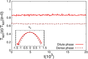
(a)

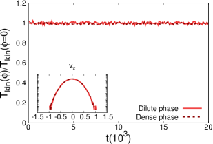
(b)

Figure 27: (Color online.) Comparison of the kinetic temperature of the two coexisting phases in the active system. We normalize the kinetic temperature with respect to the kinetic temperature of a single particle. Insets: probability distribution function of the particle velocity along one axis. ${N=256^{2}}$, ${\text{Pe}=50}$, ${\phi=0.500}$, (a) ${\gamma=10}$ and (b) $\gamma=100$.

VI Discussion

The main focus of this paper was the analysis of the effective temperature in a heterogeneous active system. More precisely, we studied the stationary dynamics of the active Brownian particle bidimensional system in (i) homogeneous situations, (ii) the co-existence region between liquid and hexatic close to the passive limit and (iii) the Mobility Induced Phase Separation (MIPS) sector of the phase diagram.

The first type of measurement that we performed was the one of the effective temperature, using the fluctuation dissipation relation, as the ratio between the mean square displacement and (twice) the time integrated linear response, either of the particles in the selected phases or in the whole system. In normal diffusion problems, this is just the Einstein ratio, that is to say, the ratio between the diffusion coefficient and the mobility. In all cases we considered sufficiently long time delays so that the dynamics is diffusive and all transients have been surpassed.

In the homogeneous phases we found a $T_{\rm eff}(\phi,\mbox{Pe})$ that at fixed Pe decays linearly with increasing packing fraction. Concerning the Pe dependence, at low density, $\phi<0.5$, $T_{\rm eff}(\phi,\mbox{Pe})$ increases as Pe², similarly to what was found in several other active systems, see e.g. Loi et al. (2008, 2011b, 2011a); Suma et al. (2014).

In the heterogeneous phases, we showed that, while in equilibrium the effective temperatures of the two phases coincide and they are equal to the bath temperature with weak deviations from this behaviour for small values of Pe, the behaviour is very different, and way more interesting, in the MIPS region at high Pe.

In the MIPS sector of the phase diagram, at fixed Pe, the global effective temperature depends on the packing fraction: at the upper limit, $\phi_{>}$, it approaches the one of the homogeneous dense phase while in the opposite limit, $\phi_{<}$, it reaches the one of the homogeneous gas. Looking more closely into the two co-existing phases, one sees that the global effective temperature can be decomposed into the contributions of the particles belonging to the dilute and dense phases, and that these are notably different. Interestingly enough, in the whole interval $[\phi_{<},\phi_{>}]$ at fixed Pe, the effective temperatures of the dilute and dense components are, within our numerical accuracy, constant and equal to the ones at the corresponding interval edges. Indeed, the curves $T_{\rm eff}(\phi)$ restricted to the particles belonging to each of the two phases, are convincingly constant not too close to the borders of the interval, while the measurements close to $\phi_{>}$ and $\phi_{<}$ become harder and harder as one of the phases disappears (the dilute one close to $\phi_{>}$, and the dense one close to $\phi_{<}$). We have therefore recovered the expectation that the effective temperature in each phase remains constant during the phase transition, but interestingly enough the temperatures of the two phases are different, being the system explicitly out of equilibrium.

Let us now compare these results to others in the literature. In particular, two studies that addressed issues linked to the effects of heterogeneities on, and observable dependencies of, the effective temperatures.

Levis and Berthier Levis and Berthier (2015) performed a spectral analysis of the effective temperature in the fluid, clustered, dense phase of a self-propelled particle model Levis and Berthier (2014) and found a non-trivial wave-vector dependence (over a factor of 2, approximately). Rightly so, these authors concluded that, contrary to what happens in glassy systems or weakly sheared liquids, a single effective temperature does not describe the dynamics of their active liquid. Instead, upon approach to a glassy arrest at very large densities, or to the dilute limit, the wave-vector dependence progressively disappears and a single $T_{\rm eff}$ value is found with different measurements in their system. These findings are in line with our results, since they also reflect the strongly heterogenous nature of the system studied Levis and Berthier (2014). A spatially resolved analysis was not conducted in this model.

Nardini et al. Nardini et al. (2017) also examined the wave vector dependence of the FDT violations in a scalar field theory with model B dynamics. We note that activity was added in this model with terms that act on the interfaces only. Interesting enough, exploiting an extension of the Harada-Sasa relation, they found that the entropy production is concentrated on the interfaces between dense and dilute regions of the samples. In our model, there is violation of FDT in the whole system, that is to say, on the boundaries but also in the bulk of the dense and dilute regions, and there should be entropy production in the latter as well.

Sobolev et al. Sobolev and Kudinov (2020) proposed an effective temperature of an active colloidal system written as the product of the single particle effective temperature extracted from the violations of the FDT and another factor that takes into account the collective motion and plays a similar role to the one of an order parameter. The difference in the effective temperatures of the coexisting phases that we found cannot be reduced to this scenario since, in our model, the drift velocity is zero in both phases. Anyway, it would be interesting to test this idea in, for example, dumbbell Gonnella et al. (2014); Suma et al. (2014); Cugliandolo et al. (2015a, b, 2017); Petrelli et al. (2018), rod Peruani (2015); Bär et al. (2020) or even Hamiltonian Bore et al. (2016); Casiulis et al. (2020) systems in which there is collective motion of the dense phase.

Having found that heterogenous active systems are characterized by two global effective temperatures, linked to the dilute and dense components, it was quite natural to complement its study with the one of local fluctuations or, more precisely, follow the statistical behavior of the individual particles.

In the homogeneous active liquid, the probability distribution functions of the displacement and integrated linear response put in normal form (that is to say, with the average subtracted and divided by the standard deviation) fall on two master curves that are independent of the global packing fraction and the strength of the activity. (The distribution of the integrated linear response for Pe = 0 and $\phi=0$ at $t_{w}=0$ has the peculiarity of not having a left wing.) Therefore, $\phi$ and Pe only affect the mean values, $\Delta^{2}$ and $\chi$.

In the heterogeneous phases, we saw that the particles separate in two populations also from the point of view of the fluctuations. The fluctuations of the square displacement and linear response of the particles in the dilute phase, once presented in normal form, coincide with the ones of the single passive particle. As in the homogeneous phases, Pe and $\phi$ affect the means $\Delta^{2}$ and $\chi$ but not the fluctuations around them. Instead, the fluctuations of the displacement of the particles in the dense phase change form. They show a Gaussian core and exponential tails both in the dense passive and active cases. The tails of the distributions of the square displacement, the linear response and the effective temperature are then modified by the changes in the statistics of $\tilde{\Delta}_{i,x}$. Therefore, in the dense phase not only the mean values, $\Delta^{2}$ and $\chi$, but also the fluctuations of these observables differ from the ones in the dilute phase.

Let us compare the fluctuations in the ABP model with the ones found in other out of equilibrium particle systems. Spatial fluctuations of the displacements, linear responses and effective temperature in glassy systems were considered in Castillo et al. (2002, 2003); Avila et al. (2013), see [Chamon and Cugliandolo, 2007] for a review. In these articles an emerging time-reparametrisation symmetry, in the long time delay relaxation dynamics, was claimed to constrain the noise induced fluctuations to be such that the global $\chi(\Delta^{2})$ parametric relation remains satisfied even locally (after coarse-graining). Solvable models with diffusive (and critical) but not glassy dynamics were considered in Corberi and Cugliandolo (2012) and the fluctuations were shown to behave differently from the ones in glassy models. The simulations we show align with the results in Corberi and Cugliandolo (2012).

In experiments Wu and Libchaber (2000); Leptos et al. (2009); Ortlieb et al. (2019) the fluctuations at the scale of microorganisms are characterized by analyzing the trajectories of colloidal tracer particles dispersed in the active fluids. In the diffusive regime, the pdf of the displacement exhibit similar features to the ones we measured: they are well fitted by the sum of a Gaussian and an exponential and they can be rescaled by their standard deviation Leptos et al. (2009). We note that no dense-dilute phase separation was reported in these experiments and that, therefore, they have most probably been performed in homogeneous phases. Similar exponential tails were observed in the statistics of the displacement of the center of mass and orientation of active dumbbells in sufficiently dense systems at intermediate and long time delays Cugliandolo et al. (2015b).

Quenched disorder in spin-glass models were shown to induce site dependent violations of the fluctuation dissipation theorem as applied to the noise averaged local correlations and linear response functions Romá et al. (2007). More precisely, in these models the spins acquire an “identity”, correlated with the backbone of the ground states, itself determined by the random interactions. The spins then separate in two population, one behaving as in the paramagnetic phase and the other behaving as in domain growth problems. Our results bear some resemblance with the ones in Romá et al. (2007) although in our problem the particles do not have a static nature, but they behave in a way or another during the given observation time interval only (they can belong to the dilute or dense phase, or they can move from one to the other).

We ended the paper with a short analysis of the kinetic temperature. The difference between this concept and the effective temperature has been extensively discussed in the context of granular and glassy systems. Here we wanted to stress the fact that the former depends on the friction coefficient while the latter does not (when the transient has been overcome and the measurements are done in the asymptotic diffusive regime). As long as the friction coefficient is not too weak the kinetic temperature of the whole system, but also the ones of the two components in heterogeneous cases, approach the single particle one with trivial Gaussian fluctuations. Therefore, one can not use the instantaneous kinetic temperature as means to study emerging thermodynamic properties of active systems.