Breaking RSA Security With A Low Noise D-Wave 2000Q Quantum Annealer:
Computational Times, Limitations And Prospects

Abstract

The RSA cryptosystem could be easily broken with large scale general purpose quantum computers running Shor’s factorization algorithm. Being such devices still in their infancy, a quantum annealing approach to integer factorization has recently gained attention. In this work, we analysed the most promising strategies for RSA hacking via quantum annealing with an extensive study of the low noise D-Wave 2000Q computational times, current hardware limitations and challenges for future developments.

I Introduction

In 1977, Ronald Rivest, Adi Shamir and Leonard Adleman proposed an algorithm for securing data, better known today with the acronym of RSA, which became the most famous and widely used algorithm in security RSA .

The core idea behind RSA comes from a well known problem in number theory, the Prime Factorization (PF) problem, stating the following.

Consider an integer $N$ which is the product of two unknown prime numbers. The task is to find the primes $p$ and $q$ such that

$$N=p\times q$$

This seemingly easy task turns out to be hard in practice, in fact it does not exist a deterministic algorithm that finds the prime factors in polynomial time Krantz ; Arora . The best classical algorithm Lenstra is able to factor an integer $N$ in a time that is

$${\displaystyle O\!\left(e^{1.9(\log N)^{1/3}(\log\log N)^{2/3}}\right)}.$$ (1)

Hence the complexity class associated to the PF problem is NP, despite not considered to be NP-complete Goldreich .

In 1994, a groundbreaking result was published by the mathematician Peter Shor Shor . He proved that a general purpose quantum computer could solve the integer factorization problem exponentially faster than the best classical algorithm. Shor’s quantum algorithm cleverly employs the quantum Fourier transform subroutine to factor an integer $N$ in a number of steps of order

$${\displaystyle O\!\left((\log N)^{2}(\log\log N)(\log\log\log N)\right)}.$$ (2)

This means that, in order to break RSA-2048, which involves the factorization of a 2048 binary digits number, the best classical algorithm would require around $10^{34}$ operations, while a quantum computer only needs $10^{8}$ quantum operations.

However, it is largely believed that a physical implementation of a fault tolerant general purpose quantum computer able to run Shor’s algorithm on large integers and break RSA-2048 is still decades away gidney2019factor .

On the other side, a large effort has been put forward in the development of annealers i.e. specific purpose quantum devices able to perform optimization and sampling tasks. In the last few years, multiple implementations of Shor-like algorithm running on quantum annealers have been proposed and tested Schaller ; Dattani ; Jiang . Still, a precise report of the running times required by the annealing hardware to factor integers is currently lacking in the literature.

In this work, we aim at analysing the most promising approaches to integer factorization via quantum annealing with an extensive investigation of the low noise D-Wave 2000Q computational times, current limitations of the hardware, opportunities and challenges for the future.

This paper is organized as follows: in the first Section, the technique of Quantum Annealing is introduced, as well as the properties of the latest D-Wave quantum annealing device. In Section III, several formulations of the factorization problem are presented. Finally, in Section IV, our approach for solving PF with the D-Wave 2000Q quantum annealer is explained and analysed in detail.

II Quantum Annealing

Several algorithms have been proposed for finding the global minimum of a given objective function with several local minima.

An example is Simulated Annealing (SA), where thermal energy is used to escape local minima and a cooling process leads the system towards low energy states SA . The transition probability between minima depends on the height $h$ of the potential well that separates them, $e^{-\frac{h}{k_{B}T}}$. Hence SA is likely to get stuck in the presence of very high barriers.

Similarly, the meta-heuristic technique known as Quantum Annealing (QA) searches for the global minimum of an objective function by exploiting quantum tunnelling in the analysis of the candidate solutions space QA .

The advantage is that the tunnelling probability depends both on the height $h$ and the width $w$ of the potential barriers, $e^{-\frac{w\sqrt{h}}{\Gamma}}$, where $\Gamma$ is the transverse field strength. This gives QA the ability to easily move in an energy landscape where local minima are separated by tall barriers, provided that they are narrow enough PhysRevX.6.031015 .

QA is strictly related to Adiabatic Quantum Computing (AQC), a quantum computation scheme where a system is initialized to the ground state of a simple Hamiltonian and then gradually turned to reach a desired problem Hamiltonian McGeoch . AQC is based on the adiabatic theorem stating that, if the quantum evolution is slow enough, the system remains in its ground state throughout the whole process.

However, while AQC assumes a unitary and adiabatic quantum evolution, QA allows fast evolution exceeding the adiabatic regime. For this reason, plus the fact that temperature is often few mK above absolute zero, QA is not guaranteed to end up the annealing process in the system ground state.

Formally speaking, the time-dependent Hamiltonian describing QA is the following

$$H(t)=A(t)H_{0}+B(t)H_{\rm P}\;,$$ (3)

where $H_{0}$ and $H_{\rm P}$ are respectively the initial and problem Hamiltonian. The annealing schedule is controlled by the functions $A(t)$ and $B(t)$, defined in the interval $t\in[0,T_{\rm QA}]$, where $T_{\rm QA}$ is the total annealing time.

The annealing process is scheduled as follows: at the beginning, the transverse field strength $A(t)$ is large i.e. $A(0)\gg B(0)$ and the evolution is governed by the $H_{0}$, responsible for quantum tunnelling effects; $A(t)$ and $B(t)$ vary in time according to the graph in Fig.1 until, at the end of the annealing, $A(T_{\rm QA})\ll B(T_{\rm QA})$ and the dominant term in the evolution is the problem hamiltonian $H_{P}$.

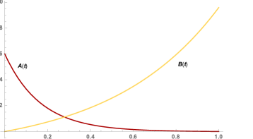
Figure 1: Plot of the smooth functions $A(t)$ (red line) and $B(t)$ (yellow line) defining the annealing schedule.

(a) D-Wave Quantum Annealer

The Canadian company D-Wave Systems is nowadays the world leading producer of quantum annealing devices which provides access to their machines via cloud. The current most advanced QA hardware is a 2048-qubit QPU going under the name of D-Wave 2000Q.

D-Wave devices solve specific combinatorial optimization problems known as Quadratic Unconstrained Binary Optimization (QUBO) problems, to which is associated an objective function of the form

$$O(x)=\sum_{i}h_{i}{x}_{i}+\sum_{i>j}J_{i,j}x_{i}x_{j}$$ (4)

with $x_{i}\in\left\{0,1\right\}$ binary variables and $h_{i}$ and $J_{ij}$ parameters whose values encode the optimization task to solve.

The D-Wave QA hamiltonian $\mathcal{H}_{QA}$ is given by

$$\begin{split}\mathcal{H}_{QA}={A(s)}\sum_{i}\hat{\sigma}^{(i)}_{x}+{B(s)}H_{P}\end{split}$$ (5)

where annealing parameters $A(s)$ and $B(s)$ are those shown in Fig.1. The problem Hamiltonian $H_{P}$ associated to the objective function $O(x)$ is expressed as an Ising hamiltonian

$$\begin{split}H_{P}=\sum_{i}h_{i}\hat{\sigma}^{(i)}_{z}+\sum_{i>j}J_{i,j}\hat{\sigma}^{(i)}_{z}\hat{\sigma}^{(j)}_{z}\end{split}$$ (6)

where $\hat{\sigma}^{(i)}_{x}$ and $\hat{\sigma}^{(i)}_{z}$ are Pauli $x$ and $z$ operators. Being $\sigma^{(i)}_{z}\in\{+1,-1\}$, it is possible to switch between Ising and QUBO problems using the relation $x_{i}=\frac{\sigma^{(i)}_{z}+1}{2}$. Hence the two formulations are perfectly equivalent, in the sense that finding the ground state energy of the Ising problem corresponds to solving the associated QUBO.

Several interesting problems can be cast into the QUBO form, examples include clustering kurihara2014quantum ; Bottarelli2018 , graph partitioning and isomorphism Lucas , map colouring Titiloye , matrix factorization ottaviani2018low but also portfolio optimization Venturelli and protein folding Perdomo .

However, a crucial aspect to take into account when using the D-Wave annealer is the embedding of the logical Ising/QUBO problem into the physical architecture of the quantum device, that we address as physical Ising problem.

This mapping is usually found via a heuristic algorithm named find_embedding, available through the D-Wave python libraries, which searches for the minor-embedding of the graph representing our problem into the target hardware graph Cai2014 . Once the mapping has been found, the D-Wave solves the embedded physical Ising problem where logical variables of the QUBO are represented as chains of physical variables (qubits). For this reason the embedding always increases the number of variables required in the optimization.

III Qubo Formulation of the prime factorization problem

Consider an integer $N$ that could be represented in binary form using $L_{N}$ bits,

$$\left\lceil log_{2}(N)\right\rceil=L_{N}$$ (7)

where $\left\lceil\cdot\right\rceil$ is the ceiling function. The PF problem asks to find the two prime factors $p$ and $q$ such that

$$N=p\times q.$$ (8)

Expressing the above numbers $N$, $p$ and $q$ in binary, the following relations are obtained

$$N=\sum_{i=0}^{L_{n}-1}2^{i}n_{i},\leavevmode\nobreak\$$ (9)

$$p=\sum_{j=0}^{L_{p}-1}2^{j}p_{j}\ \ \ \ \ \ \ \mathrm{and}\ \ \ \ \ \ \ q=\sum_{k=0}^{L_{q}-1}2^{k}q_{k}.$$ (10)

where $L_{p}$ and $L_{q}$ are respectively the bit-lengths of $p$ and $q$, while $n_{i}$, $p_{j}$ and $q_{k}\in\{0,1\}$. Since it can be proved that either

$$L_{n}=L_{p}+L_{q}\hskip 28.45274pt\mathrm{or}\hskip 28.45274ptL_{n}=L_{p}+L_{q}-1,$$

without loss of generality, the primes factors $p$ and $q$ can be chosen to be of the same length and specifically such that

$$L_{p}=L_{q}=\left\lceil L_{n}/2\right\rceil.$$ (11)

Several approaches can be followed in order to convert problems like PF into an optimization problem. Moreover, it often happens that the objective function $O(p,q)$ involves terms with order higher than two. This means that $O(p,q)$ is not in the desired QUBO form but rather it is expressed as a High-order Unconstrained Binary Optimization (HUBO) problem.

The trick used to transform HUBOs into QUBOs is to add ancillary variables and substitute high order terms with an expression having the same minimum and containing only quadratic terms Jiang . As an example, cubic term like $\pm x_{1}\cdot x_{2}\cdot x_{3}$ can be divided using the ancillary binary variable $a_{1}$ as

$$\pm x_{1}\cdot x_{2}\cdot x_{3}\ \rightarrow\ \pm a_{1}x_{3}+2(x_{1}x_{2}-2x_{1}a_{1}-2x_{2}a_{1}+3a_{1})$$ (12)

In the following, the main approaches used to convert the factorization problem into HUBOs are presented.

(A) Direct Method

A straightforward way to express PF as an optimization problem requires to consider the following objective function to minimize

$$O(p,q)=(N-p\cdot q)^{2}$$ (13)

where the square at the exponent ensures that the function has its global minimum only when $p$ and $q$ are the factors of $N$. It is possible to rewrite Eq.13 in binary form using Eq.s 9-10 as

$$O(p,q)=\left[\left(\sum_{i=0}^{L_{n}-1}2^{i}n_{i}\right)-\left(\sum_{j=0}^{L_{p}-1}2^{j}p_{j}\right)\cdot\left(\sum_{k=0}^{L_{q}-1}2^{k}q_{k}\right)\right]^{2}$$ (14)

where $n_{i}$ are known coefficients, while the $p_{j}$s and the $q_{k}$s constitute the binary unknown variables among which the objective function is minimized.

Unfortunately, using this method for factorizing larger numbers is hard because the square of $p\cdot q$ in the objective function produces many high order terms and a large number of ancillary variables are required Jiang .

(B) Multiplication Table Method

An alternative strategy Schaller to translate PF into an optimization problem involves the construction of the binary multiplication table of $p$ and $q$. Without loss of generality, we can write $p$ and $q$ in binary form using $p_{i}$ and $q_{i}\in\left\{0,1\right\}$ as

$$\begin{split}p=(1,p_{L_{p}-2},...,p_{3},p_{2},p_{1},1)\\ q=(1,q_{L_{q}-2},...,q_{3},q_{2},q_{1},1)\end{split}$$ (15)

where $p_{0}$ and $q_{0}$ are set to $1$ because $p$ and $q$ must be odd. Also the most significant digits $\ p_{L_{p}-1}=q_{L_{q}-1}=1$ to ensure $p$ and $q$ have the correct length.

Suppose $N$ to be a number with binary length $L_{N}=8$, since, by Eq.11, both $p$ and $q$ must be such that $L_{p}=L_{q}=4$, we can schematically represent Eq.s 9-10 as

$$\begin{array}[]{|c |c|c|c|c|c|c|c|c|}\hline\cr&2^{7}&2^{6}&2^{5}&2^{4}&2^{3}&2^{2}&2^{1}&2^{0}\\ \hline\cr\hline\cr p&&&&&1&p_{2}&p_{1}&1\\ \hline\cr q&&&&&1&q_{2}&q_{1}&1\\ \hline\cr N&n_{7}&n_{6}&n_{5}&n_{4}&n_{3}&n_{2}&n_{1}&n_{0}\\ \hline\cr\end{array}$$ (20)

The binary multiplication $p\cdot q$ can be visualized using the following table

$$\begin{array}[]{|c | c|c|c|c|c|c|c|c|}\hline\cr\hbox{\multirowsetup \footnotesize{Columns} }&7&6&5&4&3&2&1&0\\ \hline\cr\hline\cr\hbox{\multirowsetup \footnotesize$\mathbf{p\cdot q}$ }&&&&&1&p_{2}&p_{1}&1\\ \cline{2-9}\cr&&&&q_{1}&p_{2}q_{1}&p_{1}q_{1}&q_{1}&\\ \cline{2-9}\cr&&&q_{2}&p_{2}q_{2}&p_{1}q_{2}&q_{2}&&\\ \cline{2-9}\cr&&1&p_{2}&p_{1}&1&&&\\ \cline{2-9}\cr\hline\cr\hline\cr\hbox{\multirowsetup\footnotesize{Carries}}&c_{67}&c_{56}&c_{45}&c_{34}&c_{23}&c_{12}&&\\ &c_{57}&c_{46}&c_{35}&c_{24}&&&&\\[2.0pt] \hline\cr\hline\cr\hline\cr\footnotesize\textbf{N}&n_{7}&n_{6}&n_{5}&n_{4}&n_{3}&n_{2}&n_{1}&n_{0}\\ \hline\cr\end{array}$$ (29)

where the bitwise multiplication is performed in columns. The $c_{i,j}$ are the carries relative to column $j$ which came from the sum obtained in column $i$. Carries are calculated assuming that all bits in each column are ones.

At this stage it is possible to construct a system of equations equating the sum of each column $i$, including its carries, to the corresponding $n_{i}$ shown in the last row. In the previous example, the system of equations becomes

$$\begin{cases}p_{1}+q_{1}-2c_{12}=n_{1}\\ p_{2}+p_{1}q_{1}+q_{2}+c_{12}-(2c_{23}+4c_{24})=n_{2}\\ 1+p_{2}q_{1}+p_{1}q_{2}+1+c_{23}-(2c_{34}+4c_{35})=n_{3}\\ q_{1}+p_{2}q_{2}+p_{1}+c_{24}+c_{34}-(2c_{45}+4c_{46})=n_{4}\\ p_{2}+q_{2}+c_{45}+c_{35}-(2c_{56}+4c_{57})=n_{5}\\ 1+c_{56}+c_{46}-2c_{67}=n_{6}\\ c_{57}+c_{67}=n_{7}\end{cases}$$ (30)

The objective function is obtained considering the square of each equation in the system

$$\begin{split}&O(p,q)=\left(p_{1}+q_{1}-n_{1}-2c_{12}\right)^{2}+\\ &+\left(p_{2}+p_{1}q_{1}+q_{2}+c_{12}-n_{2}-2c_{23}-4c_{24}\right)^{2}+\ ...\ +\\ &+\left(1+c_{56}+c_{46}-n_{6}-2c_{67}\right)+\left(c_{57}+c_{67}-n_{7}\right)^{2}\end{split}$$ (31)

The HUBO obtained in this way usually contains less high order terms with respect to the Direct Method, however it is possible to further improve this strategy, as shown in the following section.

(C) Blocks Multiplication Table Method

This variation of the multiplication table method is able to reduce the number of binary variables appearing in the optimization function by performing $p\cdot q$ in blocks rather than in columns Jiang . An example is shown in the table below, for the case of $L_{p}=L_{q}=4$.

$$\begin{array}[]{|c ? c|c|c? c|c?c|c?c |}\hline\cr\hbox{\multirowsetup \footnotesize{Blocks} }\hfil\lx@intercol\vrule width=&\lx@intercol\hfil\textbf{III}\hfil\lx@intercol\vrule width=1.3pt\lx@intercol&\lx@intercol\hfil\textbf{II}\hfil\lx@intercol\vrule width=1.3pt\lx@intercol&\lx@intercol\hfil\textbf{I}\hfil\lx@intercol\vrule width=1.3pt\lx@intercol&\lx@intercol\hfil\textbf{}\hfil\lx@intercol\vrule\lx@intercol\\ \hline\cr\hline\cr\hbox{\multirowsetup \footnotesize$\mathbf{p\cdot q}$ }\hfil\lx@intercol\vrule width=&&&\hfil\lx@intercol\vrule width=&&1\hfil\lx@intercol\vrule width=&p_{2}&p_{1}\hfil\lx@intercol\vrule width=&1\\ \cline{2-9}\cr\hfil\lx@intercol\vrule width=&&&\hfil\lx@intercol\vrule width=&q_{1}&p_{2}q_{1}\hfil\lx@intercol\vrule width=&p_{1}q_{1}&q_{1}\hfil\lx@intercol\vrule width=&\\ \cline{2-9}\cr\hfil\lx@intercol\vrule width=&&&q_{2}\hfil\lx@intercol\vrule width=&p_{2}q_{2}&p_{1}q_{2}\hfil\lx@intercol\vrule width=&q_{2}&\hfil\lx@intercol\vrule width=&\\ \cline{2-9}\cr\hfil\lx@intercol\vrule width=&&1&p_{2}\hfil\lx@intercol\vrule width=&p_{1}&1\hfil\lx@intercol\vrule width=&&\hfil\lx@intercol\vrule width=&\\ \cline{2-9}\cr\hline\cr\hline\cr\hbox{\multirowsetup\footnotesize{Carries}}\hfil\lx@intercol\vrule width=&&c_{4}&c_{3}\hfil\lx@intercol\vrule width=&c_{2}&c_{1}\hfil\lx@intercol\vrule width=&&\hfil\lx@intercol\vrule width=&\\ \hline\cr\hline\cr\hline\cr\footnotesize\textbf{N}\hfil\lx@intercol\vrule width=&n_{7}&n_{6}&n_{5}\hfil\lx@intercol\vrule width=&n_{4}&n_{3}\hfil\lx@intercol\vrule width=&n_{2}&n_{1}\hfil\lx@intercol\vrule width=&n_{0}\\ \hline\cr\end{array}$$ (39)

Bold vertical lines indicates that the table is split into three non trivial blocks. The rightmost column only contains a $1$ and it is not taken into consideration since $N$ is odd and also $n_{0}$ must be a $1$. The carries again are found assuming all bits in the columns inside each block to be ones. Those generated form block I are $c_{1}$ and $c_{2}$ while those generated form block II are $c_{3}$ and $c_{4}$.

It is worth noticing that, in this example, the blocks multiplication table strategy allowed to reduce the number of carries from the 10 obtained in the previous section to just 4. This constitute a great reduction in the number of QUBO variables, especially when the number $N$ to factor becomes large.

In order to solve the problem it is necessary to sum the contributions of each block and equate it to the corresponding bits of $N$. The following system of equations is obtained for the example related the previous table.

$$\begin{cases}(p_{1}+q_{1})+2(p_{2}+p_{1}q_{1}+q_{2})-(8c_{2}+4c_{1})=n_{1}+2n_{2}\\ \\ (1+p_{2}q_{1}+p_{1}q_{2}+1+c_{1})+2(q_{1}+p_{2}q_{2}+p_{1}+c_{2})-\\ -(8c_{4}+4c_{3})=n_{3}+2n_{4}\\ \\ (q_{2}+p_{2}+c_{3})+2(1+c_{4})=n_{5}+2n_{6}+4n_{7}\end{cases}$$ (40)

The objective function is again obtained considering the square of each equation in the system 40

$$\begin{split}&O(p,q)=\left[(p_{1}+q_{1})+2(p_{2}+p_{1}q_{1}+q_{2})-(8c_{2}+4c_{1})-\right.\\ &\left.-(n_{1}+2n_{2})\right]^{2}+\left[(1+p_{2}q_{1}+p_{1}q_{2}+1+c_{1})+\right.\\ &\left.+2(q_{1}+p_{2}q_{2}+p_{1}+c_{2})-(8c_{4}+4c_{3})-(n_{3}+2n_{4})\right]^{2}+\\ &+\left[(q_{2}+p_{2}+c_{3})+2(1+c_{4})-(n_{5}+2n_{6}+4n_{7})\right]^{2}\end{split}$$ (41)

The HUBO shown in Eq.41 can be cast in the required QUBO format applying the trick of Eq.12.

When solving such problem using the D-Wave quantum annealer it is necessary to keep in mind two aspects. On one side, the device is limited in the number of logical variables it can embed while, on the other side, the range of coefficients appearing in the QUBO shouldn’t span over a range of values that is too broad. If one of these two conditions is not satisfied, the performances of the quantum annealing device could be severely affected.

As a matter of fact, from Eq.41, it is clear that the range of coefficients appearing in the optimization function strictly depends on the size of the blocks, i.e. on the number of columns contained in each block. Therefore, an appropriate choice of the blocks number and sizes should take into account for the trade-off between number of QUBO variables in play and range of the coefficients. Approximatively, an acceptable splitting into blocks makes the largest QUBO coefficient no larger than $O((log(N))^{3})$ Jiang .

IV Prime Factorization on The low noise D-Wave 2000Q

In this section, a quantum annealing approach to the problem of PF is presented and discussed.

Our aim is the study of the performances and limits of the low noise D-Wave 2000Q in addressing such problem. For this reason, we challenged the annealing device to perform a factorization of several integers $N$, gradually increasing their size, i.e. the bit-length $L_{N}$. The numbers selected for this study are shown in the table below.

N	p	q	Length of N in bits, $L_{N}$
143	13	11	8
3127	59	53	12
8881	107	83	14
59989	251	239	16
103459	337	307	17
231037	499	363	18
376289	659	571	19

Table 1: Selected numbers $N$ to factor, associated primes $p$ and $q$ and bit-length of $N$.

For each $N$ in Table 1 we applied the Block Multiplication Table method for finding its prime factors. The HUBO optimization function obtained is then transformed to QUBO via the make_quadratic function available through D-Wave dimod libraries DW . In the following, we report the properties of the QUBOs graph structure obtained varying $N$.

(A) Number of logical variables and connectivity

The number of QUBO logical variables increase polynomially with respect to $L_{N}$, as shown in Fig. 2. Also the QUBO quadratic terms seem to grow polynomially with the problem size (see Fig. 3)

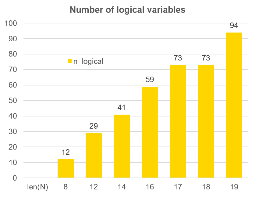
Figure 2: Number of logical variables appearing in the QUBO in relation to an increasing bit-length of $N$.

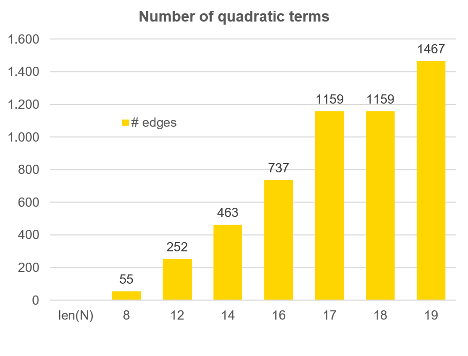
Figure 3: Number of quadratic terms (edges) appearing in the QUBO in relation to an increasing bit-length of $N$.

In the graphical representation of the QUBO, quadratic terms identifies edges between the logical variables, which constitute the nodes of the graph. An example is shown in Fig.4 where it is graphically represented the structure of the QUBO associated to the factorization of $N=143$.

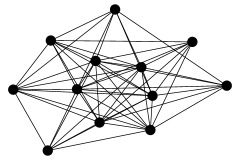
Figure 4: Graph structure of the QUBO problem related to the factorization of 143. The QUBO involves 12 binary variables (nodes) and 55 quadratic terms (edges).

The QUBO for $N=143$ involves 12 binary variables:

• $p_{1},p_{2},q_{1}$ and $q_{2}$ are those related to the factors $p$ and $q$;

• $c_{1},c_{2},c_{3}$ and $c_{4}$ are the carries;

• $a_{1},a_{2},a_{3}$ and $a_{4}$ are the ancillary variables needed to split high order terms into quadratic.

(B) Embedding

In order to use the D-Wave for the PF problem, it is necessary to embed the logical QUBOs into the actual topology of the machine. This mapping is performed via a heuristic minor-embedding approach. In Fig.5, the comparison between logical variables and the median number of physical qubits required after the embedding is reported.

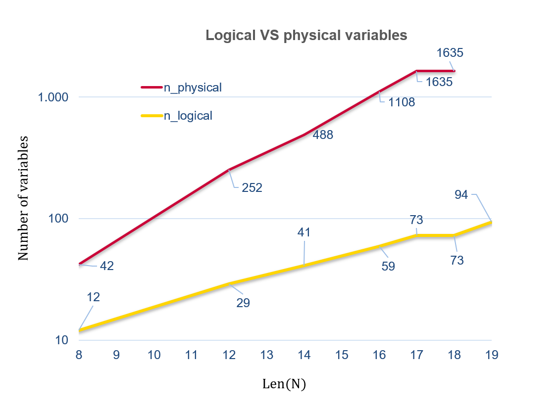
Figure 5: Comparison (in log scale) between number of logical variables in the QUBO and median number of physical variables (qubits) needed in the associated embedded Ising problem.

The D-Wave algorithm find_embedding was able to heuristically find an embedding for all instances, except for $N=376289$, i.e. $L_{N}=19$. This is due to the fact that the problem is approaching the annealer limit in the number of physical variables (qubits) required. Actually it is possible find an ad hoc manual embedding for this instance as claimed in Jiang , however, this goes beyond the purpose of our work since our aim is to test the D-Wave device both from the hardware and software perspective.

Finally, form the trends shown in Fig.5, it is clear that the gap between the number of logical variables in the QUBO and the physical qubits in the embedded Ising rapidly increases with the problem size. This currently constitute one of the main limitations of the D-Wave device which could be overcome with a more connected topology of the device. As an example, Fig.6 shows the graph of the embedded Ising problem associated to the factorization of $N=143$. The difference in complexity with respect to the logical QUBO for the same problem, shown in Fig.4, is remarkable.

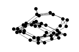
Figure 6: Graph structure of the embedded Ising problem related to the factorization of 143. The embedded problem involves 42 physical qubits (nodes) and 93 coupling terms (edges).

(C) Results

The metric used to evaluate the low noise D-Wave 2000Q device was Time To Solution (TTS) i.e. the average time, expressed in milliseconds, needed by the quantum device to find the prime factors $p$ and $q$. Such quantity is defined as follows

$$\mathrm{TTS}=\dfrac{total\ QPU\ access\ time}{number\ of\ times\ N\ is\ factored\ correctly}$$ (42)

where the total QPU access time is defined as the sum of the programming and sampling time required by the quantum annealer QPUtime . D-Wave runs have been performed in a regime of forward annealing, setting the annealing time for a single anneal to $1\mu s$ and $10000$ number of reads. Results of the computational times are reported in the graph shown in Fig.7.

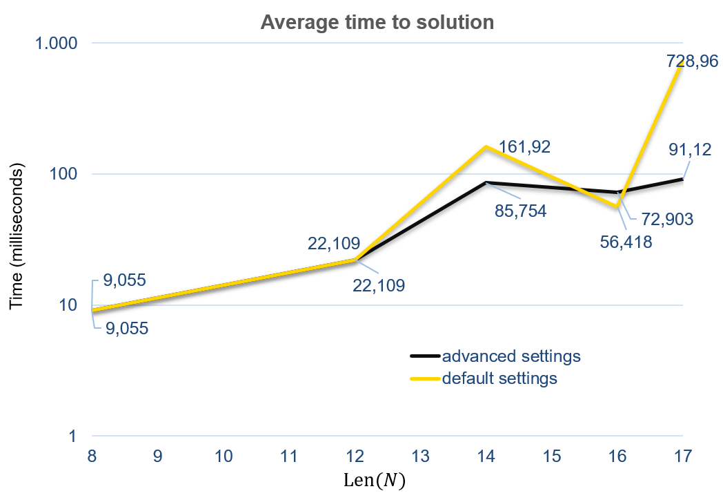
Figure 7: Time To Solution (TTS) needed for the D-Wave to output a correct solution to the factorization problem as a function of the bit-length of $N$. Solutions found using default annealing setting are identified by the yellow line; the black line shows the TTS found using advanced settings.

As a first approach, default settings of the D-Wave have been used (yellow line in Fig.7). Subsequently, advanced techniques have been used to increase the probability of solving the optimization problem. The advanced settings we selected are:

• extended J range, which enables chains of physical qubits representing a single logical variable to be coupled with an higher strength $J_{chain}=-2$ keeping all other non-chain couplings in the range $\left[-1,1\right]$;

• annealing offset, which delays the evolution of qubits applying offset in the annealing paths of the qubits, so that some are annealed slightly before others, improving performances.

The main improvement was obtained in the largest instance solved $N=103459$, i.e. $L_{N}=17$, where the TTS is decreased by almost an order of magnitude (from $728.96\mu s$ to $91.12\mu s$).

V Conclusions and Future Work

RSA RSA is a widely used cryptographic algorithm for securing data based on a fundamental number theory problem known as Prime Factorization (PF). The hardness of such problem makes harmless any attack performed by a classical computer since the computational time needed to factor a number $N$ grows exponentially with the size of $N$.

A quantum computer able to run Shor’s algorithm instead could factor the same number $N$ only in polynomial time with respect to its size Shor . Such advantage, despite being theoretically solid, can be achieved only by a large scale fault tolerant general purpose quantum computer, which is far from being built in the near term.

In recent years, a large effort has been put forward in the development of annealers, with different Shor-like quantum annealing algorithms proposed in the literature Schaller ; Dattani ; Jiang .

For this reason, with the present work, we aimed at analysing three different methods for addressing the PF problem with a quantum annealer. Among them, we selected the most advanced (block multiplication table method) to test the performances and limitations of the low noise D-Wave 2000Q quantum annealer. The device was challenged to perform a factorization of several integers $N$, gradually increasing their size, going from $L_{N}=8$ to $19$.

The heuristic algorithm Cai2014 needed to map PF into the D-Wave architecture successfully embedded problems up to $L_{N}=18$. Advanced techniques like extended J range and annealing offsets have been employed in the quantum annealing optimization in order to reach superior performances. The low noise D-Wave 2000Q factored correctly all integers $N$ up to $L_{N}=17$, with a time to solution (TTS) that never exceeded the $100$ milliseconds in the advanced setting.

The obtained results are promising, however further progresses on the quantum annealing hardware are required to factor larger numbers. The figure below (Fig.8) shows the expected number of logical variables required by the QUBO to solve PF increasing the problem size.

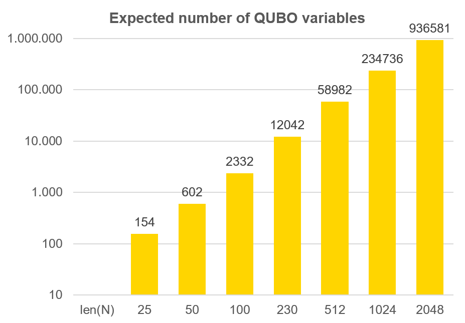
Figure 8: Expected trend of the number of QUBO logical variables needed for the factorization problem as the bit-length of $N$ increases.

It is clear that hardware improvements should focus on increasing the qubit count and connections in order to solve problems of such complexity. For this reason, it will be the subject of future studies the test of the factoring performances of the new generation D-Wave device named Advantage as well as the employment of hybrid quantum-classical techniques Peng able to divide large QUBOs into sub-problems, individually solved by quantum annealing.

References

- (1) R. L. Rivest, A. Shamir, L. Adleman, A method for obtaining digital signatures and public-key cryptosystems. Commun. ACM 21, 2, 120-126 (1978)
- (2) S. G. Krantz, The Proof is in the Pudding: The Changing Nature of Mathematical Proof, New York: Springer, 203 (2011)
- (3) S. Arora, B. Barak, Computational complexity, Cambridge: Cambridge University Press, 230(2009)
- (4) A. K. Lenstra, H. W. Lenstra, M. S. Manasse, J. M. Pollard, The number field sieve, Proceedings of the twenty-second annual ACM symposium on Theory of Computing (STOC ’90), Association for Computing Machinery, New York, NY, USA, 564-572 (1990)
- (5) O. Goldreich, A. Wigderson, IV.20 Computational Complexity, , The Princeton Companion to Mathematics, Princeton, New Jersey: Princeton University Press, 575-604 (2008)
- (6) P. W. Shor, Algorithms for quantum computation: discrete logarithms and factoring, Proceedings 35th Annual Symposium on Foundations of Computer Science, IEEE Comput. Soc. Press,124-134 (1994)
- (7) C. Gidney, M. Ekera, How to factor 2048 bit RSA integers in 8 hours using 20 million noisy qubits, arXiv 1905.09749 (2019)
- (8) G. Schaller, R. Schutzhold, The role of symmetries in adiabatic quantum algorithms, Quantum Info. Comput., 10, 1, 109-140 (2010)
- (9) N. S. Dattani, N. Bryans, Quantum factorization of 56153 with only 4 qubits, arXiv 1411.6758, (2014)
- (10) S. Jiang, K. A. Britt, A. J. McCaskey et al., Quantum Annealing for Prime Factorization, Sci Rep, 8, 17667 (2018)
- (11) S. Kirkpatrick, C. D Gelatt Jr, M. P. Vecchi, Optimization by Simulated Annealing, Science, 220 (4598), 671-680 (1983)
- (12) T. Kadowaki, H. Nishimori, Quantum annealing in the transverse Ising model, Phys. Rev. E 58, 5355 (1998)
- (13) V. S. Denchev, S. Boixo, S. V. Isakov, N. Ding, R. Babbush, V. Smelyanskiy, J. Martinis, H. Neven, What is the Computational Value of Finite-Range Tunneling?, Phys. Rev. X, 6, 031015 (2016)
- (14) C. C. McGeoch, Adiabatic Quantum Computation and Quantum Annealing: Theory and Practice, Morgan & Claypool (2014)
- (15) K. Kurihara, S. Tanaka, S. Miyashita, Quantum Annealing for Clustering, arXiv 1408.2035 (2014)
- (16) Lorenzo Bottarelli, Manuele Bicego, Matteo Denitto, Alessandra Di Pierro, Alessandro Farinelli & Riccardo Mengoni, Biclustering with a quantum annealer. Soft Comput 22, 6247-6260 (2018).
- (17) A. Lucas, Ising formulations of many NP problems, Front. Physics, 2-5 (2014)
- (18) O. Titiloye, A. Crispin, Quantum annealing of the graph coloring problem, Discrete Optimization, 8, 2, 376-384 (2011)
- (19) D. Ottaviani , A. Amendola, Low Rank Non-Negative Matrix Factorization with D-Wave 2000Q arXiv 1808.08721 (2018)
- (20) D. Venturelli, A. Kondratyev, Reverse quantum annealing approach to portfolio optimization problems. Quantum Mach. Intell., 1, 17-30 (2019)
- (21) A. Perdomo-Ortiz, N. Dickson, M. Drew-Brook et al., Finding low-energy conformations of lattice protein models by quantum annealing, Sci Rep, 2, 571 (2012).
- (22) J. Cai, B. Macready, A. Roy, A Practical Heuristic for Finding Graph Minors, arXiv 1406.2741 (2014)
- (23) https://docs.ocean.dwavesys.com/en/latest/index.html
- (24) https://docs.dwavesys.com/docs/latest/c_timing_2.html
- (25) W. Peng, B. Wang, F. Hu et al., Factoring larger integers with fewer qubits via quantum annealing with optimized parameters, Sci. China Phys. Mech. Astron., 62, 60311 (2019)