PolymoRF: Polymorphic Wireless Receivers
Through Physical-Layer Deep Learning

Abstract.

Today’s wireless technologies are largely based on inflexible designs, which makes them inefficient and prone to a variety of wireless attacks. To address this key issue, wireless receivers will need to (i) infer on-the-fly the physical-layer parameters currently used by transmitters; and if needed, (ii) change their hardware and software structures to demodulate the incoming waveform. In this paper, we introduce PolymoRF, a deep learning-based polymorphic receiver able to reconfigure itself in real time based on the inferred waveform parameters. Our key technical innovations are (i) a novel embedded deep learning architecture, called RFNet, which enables the solution of key waveform inference problems; (ii) a generalized hardware/software architecture that integrates RFNet with radio components and signal processing. We prototype PolymoRF on a custom software-defined radio platform, and show through extensive over-the-air experiments that (i) RFNet achieves similar accuracy to that of state-of-the-art yet with 52x and 8x latency and hardware reduction; (ii) PolymoRF achieves throughput within 87% of a perfect-knowledge Oracle system, thus demonstrating for the first time that polymorphic receivers are feasible and effective.

1. Introduction

It has been forecast that over 50 billion mobile devices will be soon connected to the Internet, creating the biggest network the world has ever seen (CiscoEstimates, ; EricssonMobility2018, ). However, only very recently has the community started to acknowledge that squeezing billions of devices into tiny spectrum portions will inevitably create disruptive levels of interference (pena2017internet, ). Although Mitola and Maguire first envisioned the concept of “cognitive radios” 20 years ago (mitola1999cognitive, ), today’s commercial wireless devices still use inflexible wireless standards such as WiFi and Bluetooth – and thus, are still very far from being truly real-time reconfigurable. Just to give an example of the seriousness of the spectrum inflexibility issue, DARPA has recently invested to launch the spectrum collaboration challenge (SC2), where the target is to design spectrum access schemes that “[…] best share spectrum with any network(s), in any environment, without prior knowledge, leveraging on machine-learning techniques” (DARPA-SC2, ; Yu-jsac2019, ).

From a security perspective, another key issue is perhaps even more worrisome. It has been extensively demonstrated that jamming strategies targeting the inflexibility of key components of the wireless transmission, such as headers and pilots, can significantly decrease the system throughput while increasing the jammer stealthiness. For example, Clancy (ClancyICC11, ) demonstrated that pilot nulling attacks in OFDM systems can be up to 7.5dB more effective than traditional jamming. Moreover, Vo et al. (Vo-wisec2016, ) show that short bursts across carefully-selected WiFi sub-carriers can destroy over 95% of WiFi transmissions with an energy cost three orders of magnitude less than the communicating nodes.

Intuitively, the issues of existing communication systems could be addressed by allowing transmitters to dynamically switch parameters such as carrier frequency, FFT size, and symbol modulation without coordination with the receiver. This will allow the transmitter (i) efficient spectrum occupation by using the most appropriate wireless scheme at any given moment, and (ii) change position of header and pilots over time and thus becoming less jamming-prone. Figure 1 shows an example of a polymorphic receiver able to infer the current transmitter’s physical-layer scheme (e.g., OFDM vs narrowband) and the scheme’s parameters (e.g., FFT size, channel, modulation), and then demodulate each portion of the signal.

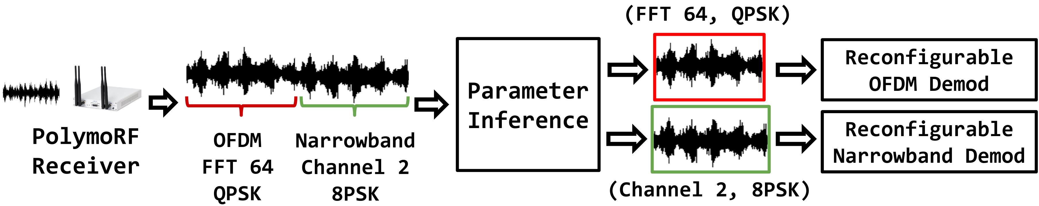
Figure 1. Example of a Self-Adaptive Polymorphic Receiver.

Doing away with explicit coordination and inflexible physical layers is the first step toward wireless receivers able to self-adapt to demodulate many waveform with a single radio interface (Restuccia-IoT2018, ; restuccia2020physical, ). Yet, despite their compelling necessity, these wireless receivers do not exist today. This manuscript aims to change the current state of affairs by proposing the first demonstration of PolymoRF, the first polymorphic wireless receiver. Achieving this goal required us to address a set of key research challenges summarized below:

(1) Keeping Up with the Transmitter. A crucial aspect is the real-time parameter inference. In practical systems, however, transmitters may choose to switch its parameter configuration in the order of milliseconds (e.g., frequency hopping, rate adaptation). For example, if the transmitter chooses to switch modulation every 100ms, the learning model should run in (much) less than 100ms (as computed in Section 4.2) to predict the parameters and morph the receiver into a new configuration. To this end, we will show in Section 5.5 that CPU latency is several orders of magnitude greater than what is required to sustain realistic sampling rates from the RF interface. Thus, we need hardware-based designs to implement low-latency knowledge extraction techniques.

(2) Creating Learning Architectures for the Embedded RF Domain. Recent advances in RF deep learning (Kulin-ieeeaccess2018, ; OShea-ieeejstsp2018, ; Karra-ieeedyspan2017, ; o2017introduction, ; o2016convolutional, ; restuccia2020deepwierl, ) have demonstrated that convolutional neural networks (ConvNets) may be applied to analyze RF data without feature extraction and selection algorithms (Xu-ieeetvt2010, ; Pawar-ieeetifs2011, ; Shi-ieeetcomm2012, ; Ghodeshar-icscn2015, ). Moreover, ConvNets present a number of characteristics (discussed in Section 3) that make them particularly desirable from a hardware implementation perspective. However, these solutions cannot be applied to implement real-time polymorphic wireless communications–as shown in Section 5.5, existing art (OShea-ieeejstsp2018, ; o2016convolutional, ) utilizes general-purpose architectures with a very high number of parameters, requiring hardware resources and latency that go beyond what is acceptable in the embedded domain. This crucial issue calls for novel, RF-specific, real-time architectures. We are not aware of learning systems tested in a real-time wireless environment and used to implement inference-based wireless systems.

(3) System-level Feasibility of Polymorphic Platforms. It is yet to be demonstrated whether polymorphic platforms are feasible and effective. This is not without a reason – from a system perspective, it required us to tightly interconnect traditionally separated components, such as CPU, RF front-end, and embedded operating system/kernel, to form a seamlessly-running low-latency learning architecture closely interacting with the RF components and able to adapt at will its hardware and software based on RF-based inference. Furthermore, since polymorphic wireless systems are subject to inference errors, we need to test its performance against a perfect-knowledge (thus, ideal and not implementable) system.

Technical Contributions

This paper’s key innovation is to finally bridge the gap between the extensive theoretical research on cognitive radios and the associated system-level challenges, by demonstrating that inference-based wireless communications are indeed feasible on off-the-shelf embedded devices. Beyond the examples and the evaluation conducted in Section 5, the main purpose of this work is to provide a blueprint for next-generation wireless receivers, where their radio hardware and software are not protocol-specific, but instead spectrum-driven and adaptable on-the-fly to different waveforms.

We summarize our main technical contributions as follows:

(1) We design a novel learning architecture called RFNet, specifically and carefully tailored for the embedded RF domain. Our key intuition in RFNet is to arrange I/Q samples to form an “image” that can be effectively analyzed by the ConvNet filters. This operation produces high-dimensional representations of small-scale transition in the I/Q complex plane, which can be leveraged to efficiently solve a wide variety of complex RF classification problems such as RF modulation classification. Extensive experimental evaluation indicates that RFNet obtains similar accuracy achieved by prior art (OShea-ieeejstsp2018, ; o2016convolutional, ), while reducing latency and hardware by 52x and 8x;

(2) We propose a general-purpose hardware/software architecture for software-defined radios that enables the creation of custom polymorphic wireless systems through RFNet. Then, we implement a multi-purpose library based on high-level synthesis (HLS) that translates an RFNet model implemented in software to a circuit implemented in the FPGA portion of the SoC. Moreover, we leverage key optimization strategies such as pipelining and unrolling to further reduce the latency of RFNet by more than 50% with respect to the unoptimized version, with only 7% increase of hardware resource consumption. Finally, we design and implement the device-tree entries and Linux drivers enabling the system to utilize RFNet and other key hardware peripherals;

(3) We prototype PolymoRF on a ZYNQ-7000 system-on-chip (SoC) and analyze its performance on a scheme where the transmitter can switch among 3 FFT sizes and 3 symbol modulation schemes without explicit notification to the receiver. A demo video of PolymoRF where the transmitter switches FFT size every 0.5s is available at https://youtu.be/5vf_pb0nvKk. We believe ours is the first demonstration of real-time OFDM reconfigurability without explicit transmitter/receiver coordination. Experiments on both line-of-sight (LOS) and non-line-of-sight (NLOS) channel conditions show that the system achieves at least 87% of the throughput of a perfect-knowledge – and thus, unrealistic – Oracle OFDM system, thus proving the feasibility of polymorphic receivers.

2. PolymorRF: An Overview

The primary operations performed by the PolymoRF platform are summarized in Figure 2. In a nutshell, PolymoRF can be considered as a full-fledged learning-based software-defined radio architecture where both the inference system and the demodulation strategy can be morphed into new configurations at will.

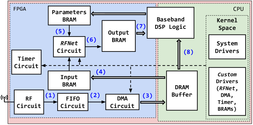
Figure 2. Modules and Operations of PolymoRF.

We provide a walk-through of the main operations performed by PolymoRF with the help of Figure 2. Although for simplicity we refer to specific hardware equipment and circuits in our explanation, we point out that the building blocks of our platform design (BRAMs, DMA, FIFOs, etc) can be implemented in any commercially-available FPGA platform.

We assume the transmitter may transmit by choosing among a discrete set of physical-layer parameters which are known at the receiver’s side. We define as $Y$ a tuple of such physical-layer parameters, which may be changed at will by the transmitter but not before $T_{sw}$ seconds between each change, which we refer to a switching time. For the sake of generality, in this paper we will not assume any particular strategy in the transmitter’s parameter choice, which can be driven by a series of factors (including anti-jamming strategy, noise avoidance, throughput optimization, and so on) that will be considered as out of the scope of this paper, whose main focus is instead on the receiver’s side.

(1) Reconfigurable Radio Front-end. The RF signal is received (step 1) through a reconfigurable RF front-end. In our prototype, we used an AD9361 (AD9361, ) radio interface, which supports frequency range between 70 MHz to 6.0 GHz and channel bandwidth between 200 kHz to 56 MHz. We chose the AD9361 because it is commonly used in software-defined radio systems – indeed, it is also used by USRPs such as the E310 and B210. Moreover, the AD9361 provides basic FPGA reference designs and kernel-space drivers to ease prototyping and extensions. Perhaps more importantly, the AD9361 local oscillator (LO) frequency and RF bandwidth can be reconfigured at will through CPU registers.

(2) Conversion from RF to FPGA domain. The AD9361 produces streams of I/Q samples of 200M samples/second – hence, it is clocked at 200 MHz. Since the AD9361 clock would be too fast for the other circuits in the FPGA, we implemented a FIFO to adapt the speed of samples from the AD9361 to the 100 MHz clock frequency used by the other circuits in the FPGA (step 2). We then use a direct memory access (DMA) core to store the stream of I/Q samples to a buffer in the DRAM (step 3). The use of DMA is crucial as the CPU cannot do the transfer itself, since it would be fully occupied for the entire duration of the read/write operation, and thus unavailable to perform other work. Therefore, we wrote a custom DMA driver to periodically fill a buffer of size $B$ residing in the DRAM with a subset of I/Q samples coming from the FIFO.

(3) Learning and Receiver Polymorphism. After the buffer has been replenished, its first $X$ I/Q samples are sent to a BRAM (step 4) constituting the input to RFNet, a novel learning architecture based on ConvNets. This circuit is the fundamental core of the PolymoRF system; therefore, we will dedicate Sections 3 and 4 to discuss in details its architecture and implementation, respectively. The parameters of RFNet are read by an additional BRAM (step 5), which in effect allows the reconfiguration of RFNet to address multiple RF problems according to the current platform need. As explained in Section 3, RFNet produces a probability distribution over the transmitter’s parameter set $Y$. After RFNet has inferred the transmitter’s parameters, it writes on a block-RAM (BRAM) its probability distribution (step 6). Then, the baseband DSP logic (which may be implemented in both hardware and software) reads the distribution from the BRAM (step 7), selects the parameter set with highest probability, and “morphs” into a new configuration to demodulate the I/Q samples in $B$ (step 8).

3. Learning System: RFNet

We first motivate the use of convolutional neural networks for RFNet, then we discuss some RF-specific learning challenges, and then we describe in details the RFNet input construction and its complete architecture.

(1) Why Using Deep Learning and not Machine Learning? Deep learning relieves from the burden of finding the right “features” characterizing a given wireless phenomenon. At the physical layer, this is a key advantage for the following reasons. First, deep learning offers high-dimensional feature spaces. In particular, O’Shea et al. (OShea-ieeejstsp2018, ) have demonstrated that on the 24-modulation dataset considered, deep learning models achieve on the average about 20% higher classification accuracy than legacy learning models under noisy channel conditions. Second, automatic feature extraction allows to reuse the same hardware circuit to address different learning problems. Critically, this allows to keep both latency and energy consumption constant, which are particularly critical in wireless systems. Third, deep learning algorithms can be fine-tuned by performing batch gradient descent on fresh input data, avoiding manual re-tuning of the feature extraction algorithms.

(1) Why Using ConvNets for Wireless Deep Learning? There are several primary advantages that make the usage of ConvNet-based models particularly desirable for the embedded RF domain. First, convolutional filters are designed to interact only with a very small portion of the input. We show in Section 5.3 that this key property allows to achieve significantly higher accuracy than traditional neural networks. Perhaps even more importantly, ConvNets are scalable with the input size. For example, for a 200x200 input and a DL with 10 neurons, a traditional neural network will have $200^{2}\cdot 10$ = 400k weights, which implies a memory occupation of $4\cdot 400$k = 16 Mbytes to store the weights of a single layer (i.e., a float number for each weight). Clearly, this is unacceptable for the embedded domain, as the network memory consumption would become intractable as soon as several DLs are stacked on top of the other.

Moreover, as we show in Section 4.2, ConvNet filtering operations can be made low-latency by parallelization, which makes them particularly suitable to be optimized for the RF domain. Finally, we show in Section 5 that the same ConvNet architectures can be reused to address different RF classification problems (e.g., modulation classification in single- and multi-carrier systems), as long as the ConvNet is provided appropriate weights through training. Our ConvNet hardware design (Section 4.1) has been specifically designed to allow seamless ConvNet reconfiguration and thus solving different RF problems according to the system’s needs.

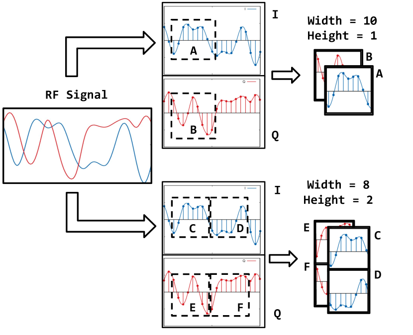
Figure 3. How RFNet constructs tensors from I/Q samples.

(2) RF-specific Learning Challenges. There are a number of key challenges in RF learning that are substantially absent in the CV domain. Among others, we know that RF signals are continuously subject to dynamic (and usually unpredictable) noise/interference coming from various sources. This may decrease the accuracy of the learning model. For example, portions of a QPSK transmission could be mistaken for 8PSK transmissions since they share part of their constellations. We address the above core design issues with the following intuitions. First, although RF signals are affected by fading/noise, in most practical cases their effect can be considered as constant over small intervals. Second, though some constellations are similar to each other, the transitions between the symbols of the constellations are distinguishable when the waveform is sampled at a higher sampling rate than the one used by the transmitter. Third, convolution operations are equivariant to translation, so they can recognize I/Q patterns regardless of where they occur.

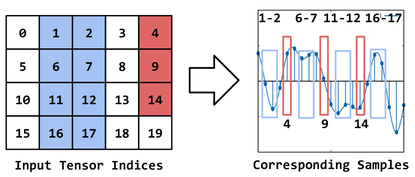
Figure 4. RFNet captures small-scale I/Q pattern sequences.

(3) RFNet Input Construction. By leveraging these key concepts, we can design a learning system that distinguishes waveforms by recognizing transitions in the I/Q complex plane regardless of where they happen, by leveraging the shift-invariance property of convolutional layers. More formally, let us consider a discrete-time complex-valued I/Q sequence $s[k]$, where $k\geq 0$. Let us consider $M=W\cdot H$ consecutive I/Q samples $s[j],\ 0\leq j\leq W\cdot H$, where $W$ and $H$ are the width and height of the input tensor. The input tensor $\mathcal{T}$, of dimension $W\times H\times 2$, is constructed as follows:

$$\mathcal{T}[r,c,d]=\mbox{Re}\left\{s[r\cdot W+c]\right\}\cdot(1-d)+$$

(1) $$\mbox{Im}\{s[r\cdot W+c]\}\cdot d,$$

$$\mbox{ where }d\in\{0,1\},0\leq r\leq H,0\leq c\leq W$$

By construction, it follows that $\mathcal{T}[r+1,c]=s[(r+1)\cdot W+c]=s[r\cdot W+c+W]$, meaning that (i) I/Q samples in adjacent columns will be spaced in time by a factor of 1, and (ii) I/Q samples in adjacent rows will be spaced in time by a factor of $W$; moreover, (iii) our input tensors have depth equal to 2, corresponding to the I and Q data, respectively, which will allow the RFNet filters to examine each element of the input tensor without decoupling the I and Q components of the RF waveform. Figure 3 depicts an example of a 2x4 and 1x3 filters operating on a waveform.

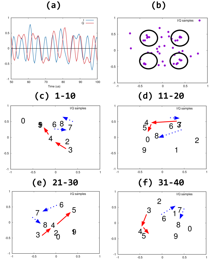
Figure 5. Example of I/Q patterns in a QPSK waveform.

To further show the intuition behind our architectural design, Figures 5(c)-(f) show the first 40 I/Q samples (ordered by occurrence) of a QPSK waveform in 5(a) which corresponds to the I/Q constellation shown in 5(b). We consider an example where $3\times 3$ filters are used, with $W=10$ and $H=4$. By setting $W$ equal to the sampling rate, we “force” the consecutive rows of the filter to recognize transitions occurring in the same portion of the symbol transmitted by the receiver. To make this point, we show in red and blue arrows the I/Q transitions “seen” by a filter applied at indices 3-4-5 and 6-7-8, respectively. While in the former case the transitions between the I/Q constellation points peculiar to QPSK can be clearly recognized, in the latter case the filter will not recognize patterns. This is because samples 3-4-5 are in between QPSK constellation points, while 7-8-9 are close to QPSK.

Figure 6 shows the complete architecture of RFNet. Similar to existing work (OShea-ieeejstsp2018, ) and computer vision-based models, the network is composed by $M$ convolutional (Conv) layers with $C$ filters each, followed by rectified linear units (ReLU) as activation functions. These are then followed by a series of dense layers, each having $D$ neurons. The final layer is a softmax output, which gives the probability distribution over the set of all possible classes.

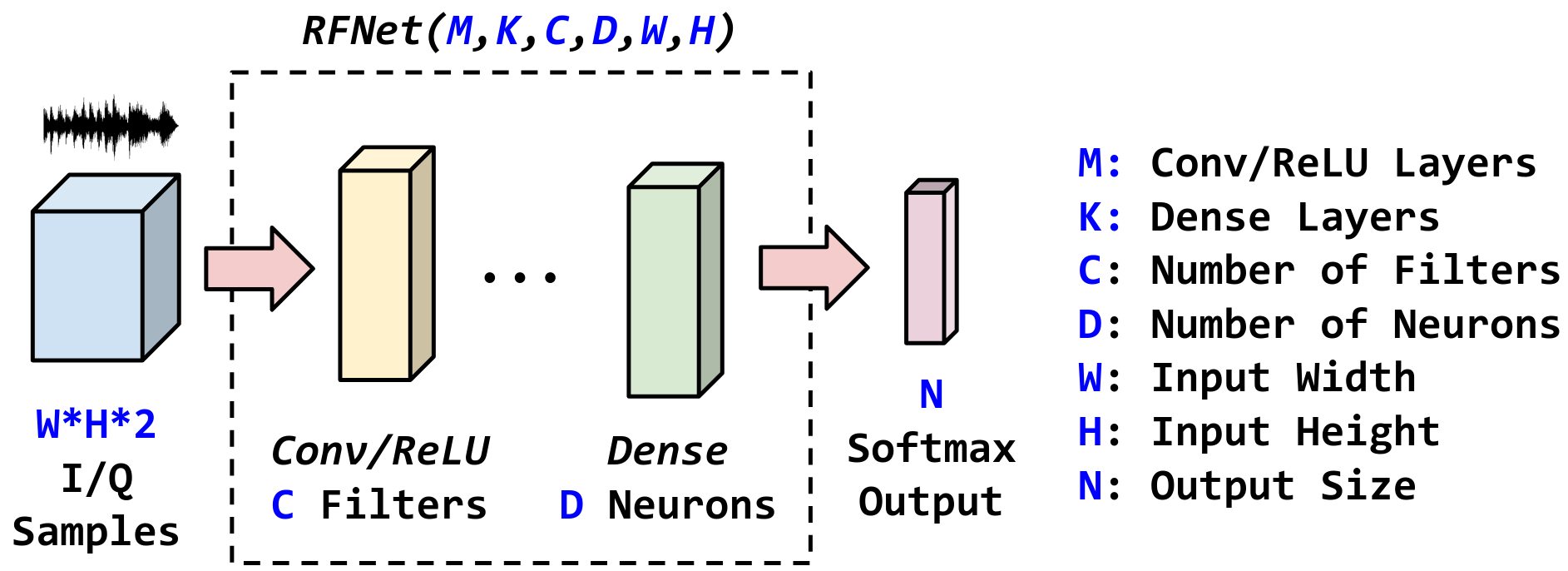
Figure 6. RFNet Architecture.

4. PolymorRF: HW/SW Architecture

This section presents the hardware and driver design and implementation of our PolymoRF system. We first discuss the design, hardware implementation and main operations of RFNet in Section 4.1, followed by a discussion of the parallelization strategies in Section 4.2 and of the Linux drivers implemented to operate the circuits in Section 4.3.

4.1. RFNet: Architecture and Operations

(1) Design Constraints. One the core design issues to address is ensuring that the same RFNet circuit can be reused for multiple learning problems and not just one architecture. For example, the wireless node might want to classify only specific properties of an RF waveform, e.g., classify only modulation since the FFT size is already known. This requires reconfigurability of the model parameters, as the device’s hardware constraints may not be able to accommodate multiple learning architectures. In other words, we want RFNet to be able to operate with a different set of filters and weight parameters according to the circumstances. For this reason, we have used high-level synthesis (HLS) to design a library that translates a Keras-compliant RFNet into an FPGA-compliant circuit. HLS is an automated design process that interprets an algorithmic description of a desired behavior (e.g., C/C++) and creates a model written in hardware description language (HDL) that can be executed by the FPGA (winterstein2013high, ).

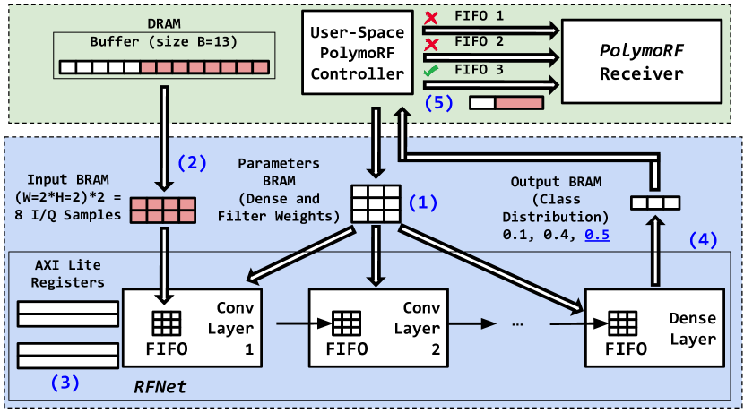
Figure 7. Block scheme of PolymoRF’s learning circuit.

(2) Circuit Design. Figure 7 shows a block scheme of our HLS-based RFNet circuit and its main interactions with the CPU and other FPGA components. We also provide an example with some numbers to ease presentation. The main feature of our RFNet implementation is its modularity – indeed, the circuits implementing each layer are independent from each other, which allows for ease of parallelization and transition from HLS to HDL. Consecutive layers in RFNet exchange data through high-speed AXI-Stream interfaces that then store the results of each layer in a FIFO, read by the next layer. Our architecture uses a 32-bit fixed-point representation for real numbers, with 10 bits dedicated to the integer portion. We chose fixed-point instead of floating-point to decrease drastically computation and hardware architecture complexity, as we do not need the precision of floating-point arithmetic. Another key advantage of our implementation is that it clearly separates the computation from the parameters, which allows for seamless real-time reconfigurability. This is achieved by writing the parameters in a BRAM accessible by the CPU and by the RFNet circuit.

(3) Main Operations. The first operation is to write the RFNet’s parameters into a BRAM through the user-space PolymoRF controller (step 1). These parameters are the weights of the convolutional layer filters and the weights of the dense layers. Since we use a fixed-point architecture, each parameter is converted into fixed-point representation before being written to the BRAM. As soon as a new input buffer $B$ (of size 13 in our example) has been replenished, the controller writes the RFNet input (the first 8 I/Q samples in our example) into the input BRAM (step 2). RFNet operations are then started by writing into an AXI-Lite register (step 3) through a customized kernel-level Linux driver. Once the results have been written in the output BRAM (step 4), RFNet writes an acknowledgement bit into another AXI-Lite register, which signals the controller that the output is ready. Then, the controller reads the output (in our example, class 3 has the highest probability), and sends the entire buffer $B$ through a Linux FIFO to the PolymoRF receiver (step 5), which is currently implemented in Gnuradio software. The receiver has different FIFOs, each for a parameter set. Whenever a FIFO gets replenished, the part of the flowgraph corresponding to that parameter set activates and demodulates the I/Q samples contained in the buffer $B$. Notice that for efficiency reasons the receiver chains do not run when the FIFO is empty, therefore only one receiver chain can be active at at time.

4.2. RFNet: Latency Optimization

We show in Section 5.5 that the above implementation on the average reduces the latency by about 95% with respect to a model implemented in the CPU. However, this performance may not be enough to sustain the flow of I/Q samples coming the RF interface. We derive some formulas to explain this critical point.

(1) Why do we need to further optimize latency? Let us suppose that the RF interface is receiving samples at $S$ samples/sec. The AD9361 quantizes I/Q samples using a 16-bit ADC, so each I/Q sample occupies 4 bytes. Therefore, the system needs to process data with throughput $4\times S$ MB/sec to keep up with the sampling rate. To process $4\cdot S$ MB of I/Q data, PolymoRF must do the following: (i) insert $B\times 8$ bytes into the DRAM through DMA; (ii) transfer the first $W\cdot H$ samples to the input BRAM; (iii) execute RFNet; (iv) read the inference from the output BRAM, for a total of $\nicefrac{{4\cdot S}}{{B\cdot 8}}=\nicefrac{{S}}{{B\cdot 2}}$ times. More formally, by defining the above quantities as $T_{buf}$, $T_{i}$, $T_{cn}$, and $T_{o}$, it must hold that $(T_{buf}+T_{i}+T_{cn}+T_{o})\cdot\nicefrac{{4\cdot S}}{{B\cdot 8}}<1$. Since our measurements show that $T_{buf},T_{i},T_{o}\ll T_{cw}$, then $T_{cn}<{2\cdot B}/{S}.$

Since sampling rate $S$ is usually fixed, to make the bound on $T_{cn}$ hold, we can either (i) increase buffer size $B$ or decrease RFNet latency $T_{cn}$. Increasing the buffer size $B$ is not desirable since an increase in buffer size implies a decrease in switching time $T_{sw}$. To give a perspective of the order of magnitude of these quantities, in our experiments $S=5$ MS/s and $T_{cn}\sim=16$ms. This implies that the buffer size $B$ must be greater than 40,000 I/Q samples, implying that RFNet inference must be valid for at least 40,000 I/Q samples, which correspond to a switching time $T_{sw}=$ 8ms.

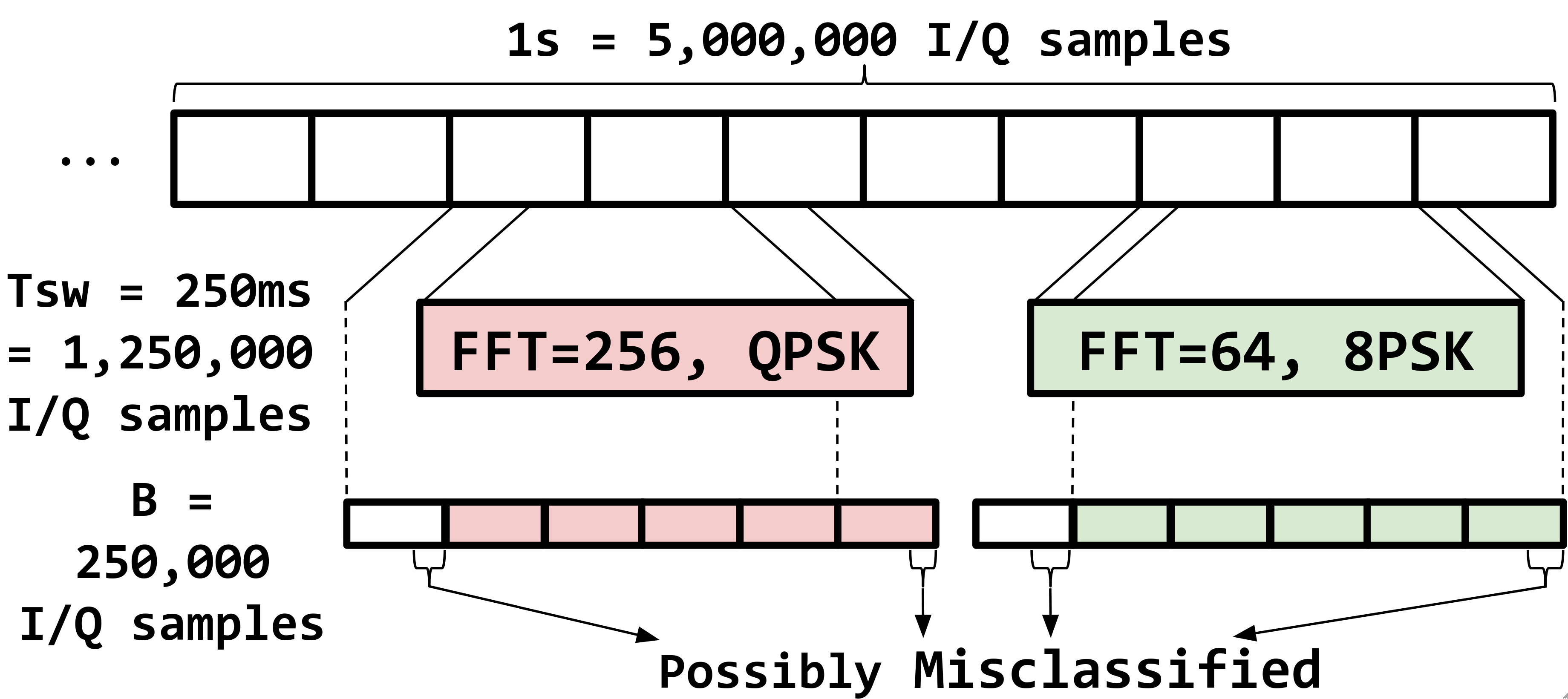
Figure 8. Switching time vs buffer size.

The calculation above assumes that it only suffices to run the model once every switching time. However, since the receiver is not aligned with the switching time, we need to run RFNet several times to obtain good performance. To help make this point, Figure 8 shows an example where some of the I/Q samples may be misclassified due to misalignment. It can be shown that the amount of I/Q samples that can be misclassified due to misalignment is approximately $B/2$ on the average, assuming all classes are equally distributed (a more precise computation would involve knowing the number of classes and their distribution). In general, having a smaller buffer $B$ is desirable as it necessarily leads to less misclassifications. The trade-off here, however, is that a smaller $B$ implies running RFNet more frequently, which leads to increased CPU usage in our current implementation. In our experiments, we run RFNet 5 times per switching time, as shown in Figure 8. This compels us to further optimize RFNet’s latency by employing FPGA parallelization techniques such as loop pipelining/unrolling.

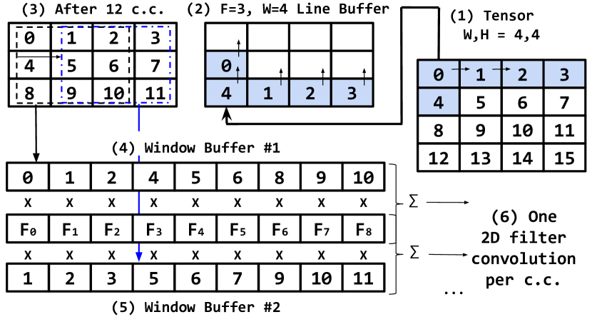
Figure 9. Example of line buffer and window buffer for 2D convolution operation.

(2) Pipelined I/Q Convolution. Arguably, the most computationally expensive operation in RFNet is the convolution between filters and input. To reduce the latency of this operation, we resort to a combination of pipelining/unrolling and line/window buffering. Figure 9 shows an example of the combined functioning of the line and window buffers, where we set for simplicity $W,H=4$ and $F=3$. In the example, I/Q samples are read one by one and inserted into the line buffer (step 1). During the insertion into the line buffer, elements are shifted vertically, while the data from the uppermost line is discarded (step 2), so as that after 12 clock cycles, the line buffer is filled (step 3). Since each line is located in a different memory location, the first window buffer can be filled by data from three line buffers in three clock cycles (step 4). The next window buffers simply discards the first column and reads the new column from the line buffers in one clock cycle. This, coupled with loop unrolling and pipelining, enables one filtering operation to be ready every clock cycle (step 5).

4.3. PolymoRF: Linux Drivers

The core challenge in designing drivers for embedded systems is that the same FPGA peripherals can change address assignment. This would require us to re-compile the kernel every time an FPGA implementation uses different physical addresses, which is obviously not acceptable. To address this key issue, we had to resort to the device tree (DT) hardware description. The DT separates the kernel from the description of the peripherals, which are instead located in a separate binary file called the device tree blob (DTB). This file is compiled from the device tree source (DTS) file, and contains not only the customized PolymoRF hardware addresses, but also every board-specific hardware peripheral information, such as the address of Ethernet, DMA, BRAMs, RF interface, and so on.

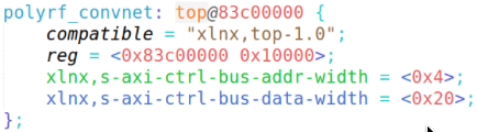
Figure 10. Device tree entry for the PolymoRF ConvNet.

For PolymoRF, we had to generate customized device-tree entries for the ConvNet, BRAM controllers, and AXI timer. Figure 10 shows the customized device tree entries in the DTS file for the input BRAM controller and RFNet (we omit the other entries due to space limitations). The most relevant entries are (i) the name of the peripheral, inserted before the ’{’ character; (ii) the reg entry, describing the starting physical address and the address space of the peripheral; and (iii) the compatible entry, which defines the ”programming model” of the device and allows the operating system to identify the corresponding device driver. Following the creation of the customized device-tree entries, we include these in the remainder portion of the global DTS file describing the ZC706 board, compile the DTB file and include it in the ZC706’s SD card containing the operating system and the kernel image.

5. Experimental Results

We first discuss details on our PolymoRF prototype in Section 5.1, and then discuss the data collection and training process in Section 5.2. We then investigate the performance of RFNet in Section 5.3 on a single-carrier system. Then, we implement and test the throughput performance on a multi-carrier polymorphic OFDM system in Section 5.4. Finally, we report the latency and hardware performance of PolymoRF in Section 5.5.

5.1. Protoype and Experimental Setup

Our prototype is entirely based on off-the-shelf equipment. Specifically, we use a Xilinx Zynq-7000 XC7Z045-2FFG900C system-on-chip (SoC), which is a circuit integrating CPU, FPGA and I/O all on a single substrate (Molanes-ieeetie2018, ). We chose an SoC since it provides significant flexibility in the FPGA portion of the platform, thus allowing us to fully evaluate the trade-offs during system design. Moreover, the Zynq-7000 fully supports embedded Linux, which in effect makes the ZC706 a good prototype for a wireless platform. Our Zynq-7000 contains two ARM Cortex-A9 MPCore CPUs and a Kintex-7 FPGA (Zynq, ), running on top of a Xilinx ZC706 evaluation board (ZC706, ).

For both intra-FPGA and FPGA-CPU data exchange, we use the Advanced eXtensible Interface (AXI) bus specification (XilinxAXI, ). In the AXI standard, data is exchanged during read or write transactions. In each transaction, the AXI master is charged with initiating the transfer; the AXI slave, in turn, is tasked with responding to the AXI master with the result of the transaction (i.e., success/failure). An AXI master can have multiple AXI slaves, and vice versa, according to the specific FPGA design. Multiple AXI masters/slaves can communicate with each other by using AXI interconnects. Specifically, AXI-Lite is used for register access and configure the circuits inside the FPGA, while AXI-Stream is used to transport high-bandwidth streaming data inside the FPGA. AXI-Full is instead used by the CPU to read/write consecutive memory locations from/to the FPGA.

To study PolymoRF under realistic channel environments, we have used the experimental setup shown in Figure 11. These scenarios investigate a line-of-sight (LOS) configuration where the transmitter is placed approximately 3m from the receiver, and a challenging non-line-of-sight (NLOS) channel condition where the transmitter is placed at 7m from the receiver and in the presence of several obstacles between them. Thus, the experiments were performed in a contested wireless environment with severe interference from nearby WiFi devices as well as multipath effect.

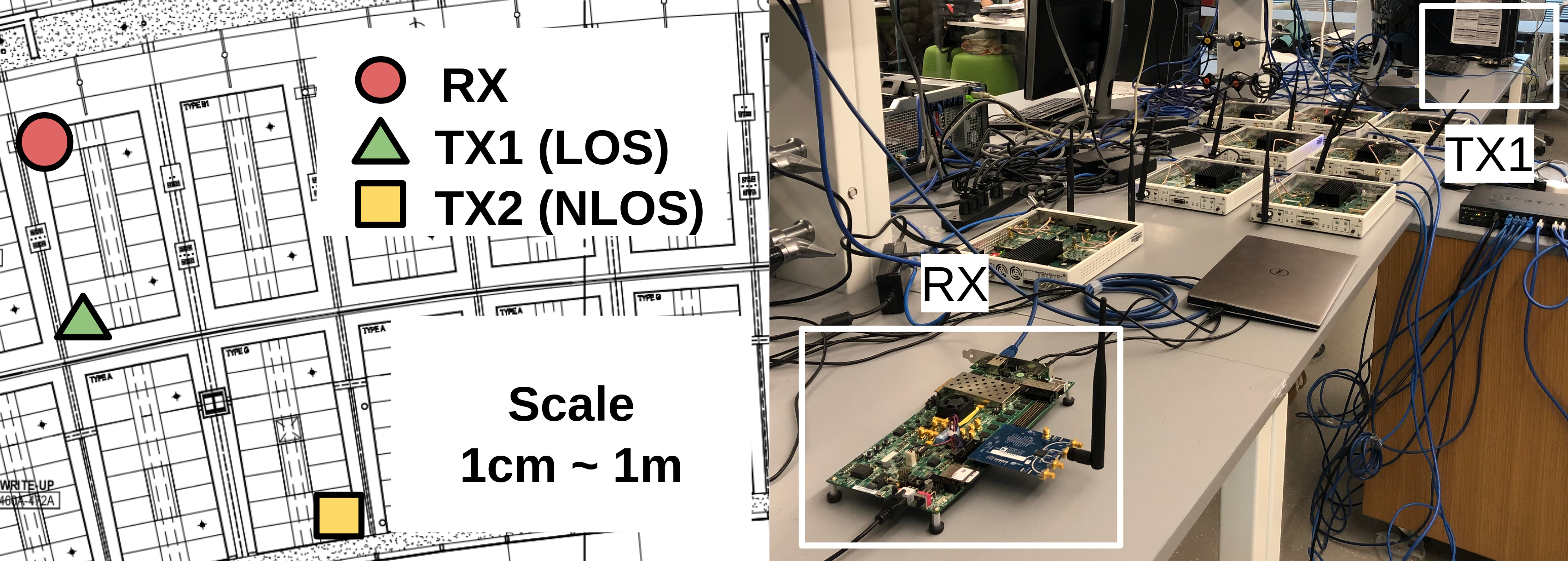
Figure 11. (left) Placement of the radios for experimental evaluation; (right) Experimental setting.

5.2. Data Collection and Training Process

As far as the data collection and testing process is concerned, we first constructed a $\sim$10GB dataset by collecting waveform data in the line-of-sight (LOS) configuration, then used this data to train RFNet through Keras. Then, we tested our models on live-collected data in both LOS and NLOS conditions. The transmitter radio used was a Zedboard equipped with an AD9361 as RF front-end and using Gnuradio for baseband processing. Waveforms were transmitted at center frequency of $2.432\ \textrm{GHz}$ (i.e., WiFi’s channel 5).

To train RFNet, we use an $\ell_{2}$ regularization parameter $\lambda=0.0001$. We also use an Adam optimizer with a learning rate of $l=10^{-4}$ and categorical cross-entropy as a loss function. All architectures are implemented in Python, on top of the Keras framework and with Tensorflow as the backend engine.

5.3. Single-carrier Evaluation

We consider the challenging problem of joint modulation and channel recognition in a single-carrier system where (i) modulation is chosen among BPSK, QPSK, 8PSK, 16-QAM, 32-QAM, and 64-QAM; (ii) spectrum is shifted of 0, 1 KHz and 2 KHz from its center frequency. Due to space limitations, we only report results on the LOS scenario for the single-carrier scenario, and report in Section 5.4 the performance of RFNet on the NLOS scenario with the multi-carrier OFDM system.

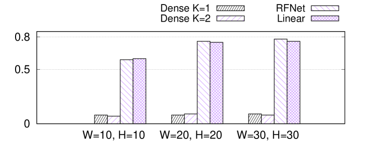
Figure 12. Comparison among RFNet, Dense and Linear (o2016convolutional, ).

(1) Comparison with Existing Architectures. We compare RFNet to (o2016convolutional, ; OShea-ieeejstsp2018, ), which is to the best of our knowledge (o2016convolutional, ; OShea-ieeejstsp2018, ) the current state of the art in RF waveform classification using ConvNets. This approach, called for simplicity Linear, considers an input tensor of dimension $1\times W\cdot H\times 2$ and convolutional layers with filters of dimension $1\times F\times 2$. Thus, the filters in the first convolutional layer perform linear convolution over a set of $F$ consecutive I/Q samples. We attempted to train the architecture in (OShea-ieeejstsp2018, ), which has M = 7 convolutional layers with C=64 filters each and K=2 dense layers with 128 neurons each. However, due to its huge dimensions, we were not able to synthesize this architecture on our testbed. Therefore, we compared RFNet with the architecture in (o2016convolutional, ), i.e., M=2 convolutional layers with C=256,80 and K=1 with 256 neurons. For fair comparison with Linear, we selected the closest input size to ours (i.e., 1x128 vs 10x10, 1x400 vs 20x20, 1x900 vs 30x30).

Figure 12 shows the test-set accuracy obtained for a subset of the considered architectures, where RFNet was trained with $M=1$ convolutional layer with $C=25$ filters, and no dense layer ($K=0$). The obtained results indicate that traditional dense networks cannot recognize complex RF waveforms, as they attain slightly more accuracy (8%) than the random-guess accuracy (5.5%) – regardless of the number of layers. This is because dense layers are not able to capture localized, small-scale I/Q variations in the input data, which is instead done by convolutional layers. Moreover, Figure 12 indicates that RFNet has similar accuracy as obtained by Linear, despite using a much simpler architecture. This is due to the fundamental difference between how the convolutional layers in PolymoRF and Linear process I/Q samples.

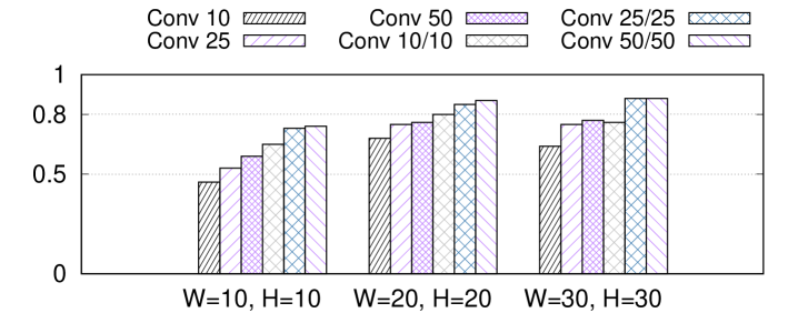
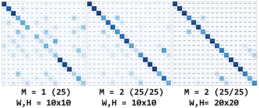
Figure 13. (top) Test-set classification accuracy vs input size $W$/$H$ vs $M$, with $K=0$ (no dense layer); (bottom) Confusion matrices as function of $M$, $W$ and $H$.

(2) Hyper-parameter Evaluation. We study the impact of the number of convolutional layers $M$ and dense layers $K$, as well as the input size ($W$) and filter size ($F$) on the performance of RFNet. Figure 13 shows accuracy as a function of $W$ and $H$, for hyper-parameters M = 1, 2 and C = 10, 25, 50. The results conclude that increasing $C$ does improve the performance but up to a certain extent. Indeed, we notice that switching to $C=50$ does not improve much the performance, especially when $M=2$. This is because the number of distinguishing I/Q patterns is limited in number among different modulations, and thus the filters in excess end up learning similar patterns. Furthermore, increasing $W$ and $H$ increases accuracy significantly, since a larger input size allows to compensate for the adverse channels/noise conditions. Furthermore, Figure 14 illustrates the impact of $K$. Figure 14 suggests that the accuracy does not increase when adding a dense layer, regardless of its size, which indicates the correctness of our choice to exclude dense layers.

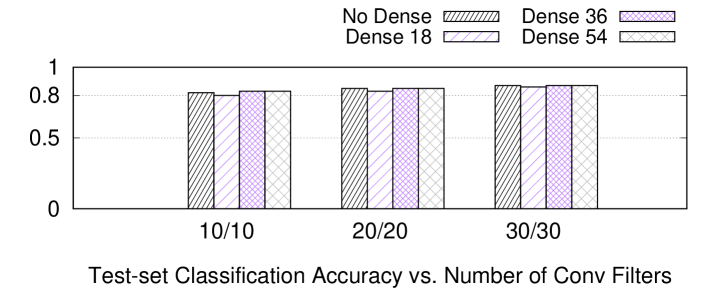
Figure 14. Accuracy vs number of filters vs dense layer size.

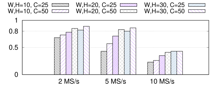
Figure 15. Accuracy vs transmitter’s sampling rate.

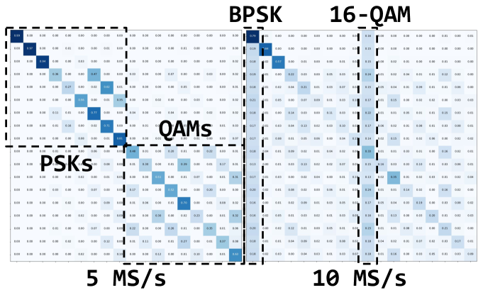
Figure 16. Confusion matrices for transmitter’s sampling rate of 5 MS/s and 10 MS/s, W,H=10, C=50 model.

(3) Impact of the Sampling Rate. We investigate the impact of the transmitter’s sampling rate in Figure 15, where we show the classification accuracy for different W, H and C values. We also show the confusion matrices for the W,H=10, C=50 architectures in Figure 16. As expected, these results confirm that the performance of RFNet decreases as the transmitter’s sampling rate increases. This is because, as shown in Section 3 RFNet learns the I/Q transitions between the different modulations. Therefore, as the transmitter’s sampling rate increases, the model will have fewer I/Q samples between the constellation points. Indeed, the confusion matrices show that with 5 MS/s the model becomes further confused with QAM constellations, and with 10 MS/s higher-order PSKs and QAMs “collapse” onto the lowest-order modulations.

(4) Remarks. The above results imply that oversampling the signal leads to a better modulation classification accuracy. However, we would like to point out that oversampling does not mean that the physical-layer has to process more data – indeed, the extra samples can be dropped when going through the demodulation chain while the oversampled I/Q signal can be forwarded to RFNet for classification.

5.4. Multi-carrier Evaluation

We evaluated PolymoRF on an OFDM system (in short, Poly-OFDM) which supports 3 different FFT sizes (64, 128, 256) and 3 different symbol modulations in the FFT bins (BPSK, QPSK, 8PSK), creating in total a combination of 9 different parameter set which are switched pseudo-randomly by the transmitter. A demo video where the transmitter switches FFT size every 0.5s is available at https://youtu.be/5vf_pb0nvKk. In the following, we use the C=25,25, 20x20, pipelined RFNet architecture, which presents latency of about 17ms (see Section 5.5). In these experiments, we set (i) the transmitter’s sampling rate to 5M samples/sec; PolymoRF’s buffer size $B$ to 250k I/Q samples; (iii) the switching time of the transmitter to 250ms. Thus, RFNet is run approximately 5 times during each switching time (see Section 4.2).

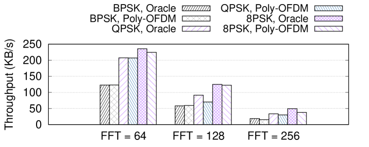
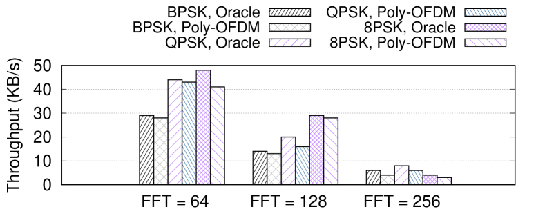
Figure 17. Comparison between Oracle and Poly-OFDM, (top) LOS and (bottom) NLOS scenarios.

The most critical aspect to be evaluated is how Poly-OFDM, an inference-based system, compares with an ideal system that has perfect knowledge of the modulation and FFT size being used by the transmitter at each time, which we call for simplicity Oracle. Although Oracle cannot be implemented in practice, we believe this experiment is crucial to understand what is the throughput loss with respect to a system where the physical-layer configuration is known a priori. Figure 17, where we show the comparison between Oracle and Poly-OFDM as a function of the FFT size and the symbol modulation. As we notice, the overall throughput results decrease in the NLOS scenario, which is expected given the impairments imposed by the challenging channel conditions. On the other hand, the results in Figure 17 confirm that Poly-OFDM is able to obtain similar throughput performance with that of a traditional OFDM system, obtaining on the average 90% and 87% throughput of that of the traditional system.

5.5. RFNet Latency Evaluation and Comparison

Table 1 compares latency, number of parameters, and BRAM occupation of RFNet vs (i) a C++ implementation running in the CPU of our testbed; and (ii) existing work (o2016convolutional, ). We were not able to synthesize the 1x900 architecture, since it was too large for our hardware. As we can see, RFNet is able to significantly reduce latency and memory occupation with respect to existing work. Indeed, we have a decrease of an order of magnitude in almost every considered scenario. Table 2 shows the comparison between the pipelined version of the ConvNet circuits and the CPU latency, as well as the look-up table (LUT) consumption increase with respect to the unpipelined version. Table 2 concludes that on the average, our parallelization strategies bring close to $60\%$ and $100\%$ latency reduction with respect to the unoptimized and CPU versions, respectively, with a LUT utilization increase of about 7% on the average.

Model	Input	Latency	Params	BRAM
RFNet C=50	10x10	5.835ms	$\sim$23k	3%
	20x20	53.11ms	$\sim$90k	14%
	30x30	233.3ms	$\sim$203k	29%
RFNet C=25,25	10x10	6.704ms	$\sim$10k	2%
	20x20	38.41ms	$\sim$17k	8%
	30x30	144.9ms	$\sim$34k	17%
RFNet C=50,50	10x10	21.41ms	$\sim$31k	4%
	20x20	100.3ms	$\sim$40k	16%
	30x30	336.9ms	$\sim$81k	34%
Linear	1x128	579.8ms	$\sim$2M	16%
	1x400	2,026ms	$\sim$8M	64%

Table 1. Latency/hardware consumption evaluation.

Model	Input	CPU	Pipelined	LUT
RFNet C=25	10x10	49.31ms	1.19ms	+3%
	20x20	478.4ms	8.077ms	+7%
	30x30	1592ms	25.54ms	+9%
RFNet C=50	10x10	106.4ms	2.381ms	+6%
	20x20	934.2ms	16.15ms	+12%
	30x30	3844ms	63.81ms	+20%
RFNet C=25,25	10x10	122.1ms	3.959ms	+1%
	20x20	677.9ms	16.29ms	+4%
	30x30	2354ms	49.57ms	+7%
RFNet C=50,50	10x10	363.9ms	13.51ms	+2%
	20x20	1826ms	48.87ms	+7%
	30x30	5728ms	131.7ms	+11%

Table 2. Pipelined vs CPU latency.

To give the reader a perspective of the amount of resources consumed on the FPGA, Figure 18 shows the FPGA implementation of respectively 10x10 and 20x20 RFNet model, both pipelined and with C=25,25 architecture, where we highlight and color the resource consumption of RFNet with respect to the AD9361 circuitry. Figure 18 indicates that the resource consumption of the RFNet circuit is significantly lesser than the AD9361 one in the 10x10 case, and becomes comparable with the 20x20 architecture. In any case, the overall resource consumption of our FPGA designs is about 50% of the total FPGA resources.

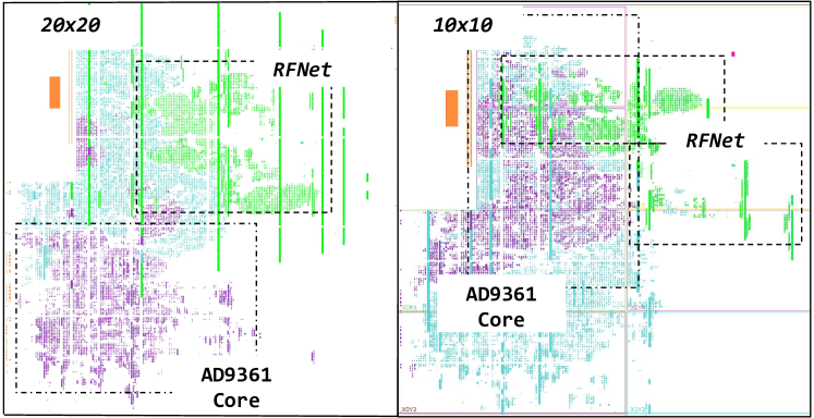
Figure 18. PolymoRF FPGA implementations.

6. Related Work and Conclusions

Learning-based radios are envisioned to be able to automatically infer the current spectrum status in terms of occupancy (subramaniam2015spectrum, ), interference (chen2016survey, ) and malicious activities (jin2018specguard, ). Most of the existing work is based on low-dimensional machine learning (Pawar-ieeetifs2011, ; Shi-ieeetcomm2012, ; Ghodeshar-icscn2015, ; xiong2019robust, ), which requires the cumbersome manual extraction of very complex, ad hoc features from the waveforms. For this reason, deep learning has been proposed as a viable alternative to traditional learning techniques (Mao-ieeecomm2018, ). The key problem of RF modulation recognition through deep learning has been extensively investigated (OShea-ieeejstsp2018, ; o2017introduction, ; wang2017deep, ; West-dyspan2017, ; Kulin-ieeeaccess2018, ; Karra-ieeedyspan2017, ). The seminal work by O’Shea et al. (OShea-ieeejstsp2018, ) and Karra et al. (Karra-ieeedyspan2017, ) proposed ConvNets-based to address the issue. However, the authors do not address the issue of what to do with the inferred RF information. Conversely, Kulin et al. present in (Kulin-ieeeaccess2018, ) a framework for end-to-end wireless deep learning, where a use case on dynamic spectrum access is provided. The above work proposes models leveraging a significant number of parameters, thus ultimately not applicable to real-time RF settings. Recently, (Restuccia-infocom2019, ) has demonstrated the need for real-time hardware-based RF deep learning. However, the main limitation of (Restuccia-infocom2019, ) is that it focus on the learning aspect only, ultimately not addressing the problem of connecting real-time inference with receiver reconfigurability.

Summary and Ongoing Work. This paper has proposed PolymoRF, a prototype that can be reused to develop and test novel polymorphic wireless communication systems. One of the key insights brought by our experimental evaluation is that the RF channel may impact the performance of RFNet to a significant extent. To this end, we can (i) train different learning models for different channels and reconfigure the weights of RFNet in the FPGA accordingly; (ii) apply small, controlled modifications to the RF signal at the transmitter’s side to compensate the current RF channel condition. Another core aspect is the impact of polymorphism on the effectiveness of smart jamming attacks. We are conscious that the above issues are definitely worth investigating, however they deserve separate papers and are the subject of our ongoing work.

7. Acknowledgements

This work is supported in part by the Office of Naval Research (ONR) under contracts N00014-18-9-0001. The views and conclusions contained herein are those of the authors and should not be interpreted as necessarily representing the official policies or endorsements of the ONR or the U.S. Government.

References

- (1) Cisco Systems, “Cisco Visual Networking Index: Global Mobile Data Traffic Forecast Update, 2016-2021 White Paper,” http://tinyurl.com/zzo6766, 2017.
- (2) Ericsson Incorporated, “Ericsson Interim Mobility Report, February 2018,” https://www.ericsson.com/assets/local/mobility-report/documents/2018/emr-interim-feb-2018.pdf, 2018.
- (3) M. D. V. Peña, J. J. Rodriguez-Andina, and M. Manic, “The Internet of Things: The Role of Reconfigurable Platforms,” IEEE Industrial Electronics Magazine, vol. 11, no. 3, pp. 6–19, 2017.
- (4) J. Mitola and G. Q. Maguire, “Cognitive Radio: Making Software Radios More Personal,” IEEE Personal Communications, vol. 6, no. 4, pp. 13–18, 1999.
- (5) Defense Advanced Research Projects Agency (DARPA), “Spectrum Collaboration Challenge – Using AI to Unlock the True Potential of the RF Spectrum,” https://www.spectrumcollaborationchallenge.com/, 2017.
- (6) Y. Yu, T. Wang, and S. C. Liew, “Deep-Reinforcement Learning Multiple Access for Heterogeneous Wireless Networks,” IEEE Journal on Selected Areas in Communications, vol. 37, no. 6, pp. 1277–1290, 2019.
- (7) T. C. Clancy, “Efficient OFDM Denial: Pilot Jamming and Pilot Nulling,” in Proc. of IEEE International Conference on Communications (ICC), 2011.
- (8) T. D. Vo-Huu, T. D. Vo-Huu, and G. Noubir, “Interleaving Jamming in Wi-Fi Networks,” in Proc. of ACM Conference on Security & Privacy in Wireless and Mobile Networks (WiSec), 2016.
- (9) F. Restuccia, S. D’Oro, and T. Melodia, “Securing the Internet of Things in the Age of Machine Learning and Software-Defined Networking,” IEEE Internet of Things Journal, vol. 5, no. 6, pp. 4829–4842, Dec 2018.
- (10) F. Restuccia and T. Melodia, “Physical-Layer Deep Learning: Challenges and Applications to 5G and Beyond,” arXiv preprint arXiv:2004.10113, 2020.
- (11) M. Kulin, T. Kazaz, I. Moerman, and E. D. Poorter, “End-to-End Learning From Spectrum Data: A Deep Learning Approach for Wireless Signal Identification in Spectrum Monitoring Applications,” IEEE Access, vol. 6, pp. 18 484–18 501, 2018.
- (12) T. J. O’Shea, T. Roy, and T. C. Clancy, “Over-the-Air Deep Learning Based Radio Signal Classification,” IEEE Journal of Selected Topics in Signal Processing, vol. 12, no. 1, pp. 168–179, 2018.
- (13) K. Karra, S. Kuzdeba, and J. Petersen, “Modulation Recognition Using Hierarchical Deep Neural Networks,” in Proc. of IEEE International Symposium on Dynamic Spectrum Access Networks (DySPAN), 2017.
- (14) T. J. O’Shea and J. Hoydis, “An Introduction to Deep Learning for the Physical Layer,” IEEE Transactions on Cognitive Communications and Networking, vol. 3, no. 4, pp. 563–575, 2017.
- (15) T. J. O’Shea, J. Corgan, and T. C. Clancy, “Convolutional Radio Modulation Recognition Networks,” in International Conference on Engineering Applications of Neural Networks. Springer, 2016, pp. 213–226.
- (16) F. Restuccia and T. Melodia, “DeepWiERL: Bringing Deep Reinforcement Learning to the Internet of Self-Adaptive Things,” Proc. of IEEE Conference on Computer Communications (INFOCOM), 2020.
- (17) J. L. Xu, W. Su, and M. Zhou, “Software-Defined Radio Equipped With Rapid Modulation Recognition,” IEEE Transactions on Vehicular Technology, vol. 59, no. 4, pp. 1659–1667, 2010.
- (18) S. U. Pawar and J. F. Doherty, “Modulation Recognition in Continuous Phase Modulation Using Approximate Entropy,” IEEE Transactions on Information Forensics and Security, vol. 6, no. 3, pp. 843–852, 2011.
- (19) Q. Shi and Y. Karasawa, “Automatic Modulation Identification Based on the Probability Density Function of Signal Phase,” IEEE Transactions on Communications, vol. 60, no. 4, pp. 1033–1044, April 2012.
- (20) S. Ghodeswar and P. G. Poonacha, “An SNR Estimation Based Adaptive Hierarchical Modulation Classification Method to Recognize M-ary QAM and M-ary PSK Signals,” in Proc. of International Conference on Signal Processing, Communication and Networking (ICSCN), 2015.
- (21) Analog Devices Incorporated, “AD9361 RF Agile Transceiver Data Sheet,” http://www.analog.com/media/en/technical-documentation/data-sheets/AD9361.pdf, 2018.
- (22) F. Winterstein, S. Bayliss, and G. A. Constantinides, “High-level Synthesis of Dynamic Data Structures: A Case Study using Vivado HLS,” in Proc. of International Conference on Field-Programmable Technology (FPT), 2013.
- (23) R. F. Molanes, J. J. Rodríguez-Andina, and J. Fariña, “Performance Characterization and Design Guidelines for Efficient Processor - FPGA Communication in Cyclone V FPSoCs,” IEEE Transactions on Industrial Electronics, vol. 65, no. 5, pp. 4368–4377, 2018.
- (24) Xilinx Inc., “Zynq-7000 SoC Data Sheet: Overview,” https://www.xilinx.com/support/documentation/data_sheets/ds190-Zynq-7000-Overview.pdf, 2018.
- (25) ——, “ZC706 Evaluation Board for the Zynq-7000 XC7Z045 All Programmable SoC User Guide,” https://www.xilinx.com/support/documentation/boards_and_kits/zc706/ug954-zc706-eval-board-xc7z045-ap-soc.pdf, 2018.
- (26) ——, “AXI Reference Guide, UG761 (v13.1) March 7, 2011,” https://www.xilinx.com/support/documentation/ip_documentation/ug761_axi_reference_guide.pdf, 2011.
- (27) S. Subramaniam, H. Reyes, and N. Kaabouch, “Spectrum Occupancy Measurement: an Autocorrelation based Scanning Technique using USRP,” in Proc. of IEEE Annual Wireless and Microwave Technology Conference (WAMICON), 2015.
- (28) Y. Chen and H.-S. Oh, “A Survey of Measurement-Based Spectrum Occupancy Modeling for Cognitive Radios,” IEEE Communications Surveys & Tutorials, vol. 18, no. 1, pp. 848–859, 2016.
- (29) X. Jin, J. Sun, R. Zhang, Y. Zhang, and C. Zhang, “SpecGuard: Spectrum Misuse Detection in Dynamic Spectrum Access Systems,” IEEE Transactions on Mobile Computing, vol. 17, no. 12, pp. 2925–2938, Dec 2018.
- (30) W. Xiong, P. Bogdanov, and M. Zheleva, “Robust and Efficient Modulation Recognition Based on Local Sequential IQ Features,” in Proc. of IEEE Conference on Computer Communications (INFOCOM), 2019.
- (31) Q. Mao, F. Hu, and Q. Hao, “Deep Learning for Intelligent Wireless Networks: A Comprehensive Survey,” IEEE Communications Surveys & Tutorials, vol. 20, no. 4, pp. 2595–2621, 2018.
- (32) T. Wang, C.-K. Wen, H. Wang, F. Gao, T. Jiang, and S. Jin, “Deep Learning for Wireless Physical Layer: Opportunities and Challenges,” China Communications, vol. 14, no. 11, pp. 92–111, 2017.
- (33) N. E. West and T. J. O’Shea, “Deep Architectures for Modulation Recognition,” in Proc. of IEEE International Symposium on Dynamic Spectrum Access Networks (DySPAN), 2017.
- (34) F. Restuccia and T. Melodia, “Big Data Goes Small: Real-Time Spectrum-Driven Embedded Wireless Networking Through Deep Learning in the RF Loop,” in Proc. of IEEE Conference on Computer Communications (INFOCOM), 2019.