Inertial Stochastic PALM (iSPALM) and Applications in Machine Learning

Abstract

Inertial algorithms for minimizing nonsmooth and nonconvex functions as the inertial proximal alternating linearized minimization algorithm (iPALM) have demonstrated their superiority with respect to computation time over their non inertial variants. In many problems in imaging and machine learning, the objective functions have a special form involving huge data which encourage the application of stochastic algorithms. While algorithms based on stochastic gradient descent are still used in the majority of applications, recently also stochastic algorithms for minimizing nonsmooth and nonconvex functions were proposed.

In this paper, we derive an inertial variant of a stochastic PALM algorithm with variance-reduced gradient estimator, called iSPALM, and prove linear convergence of the algorithm under certain assumptions. Our inertial approach can be seen as generalization of momentum methods widely used to speed up and stabilize optimization algorithms, in particular in machine learning, to nonsmooth problems. Numerical experiments for learning the weights of a so-called proximal neural network and the parameters of Student-$t$ mixture models show that our new algorithm outperforms both stochastic PALM and its deterministic counterparts.

1 Introduction

Recently, duality concepts were successfully applied for minimizing nonsmooth and nonconvex functions appearing in certain applications in image and data processing. A frequently applied algorithm in this direction is the proximal alternating linearized minimization algorithm (PALM) by Bolte, Teboulle and Sabach [4] based on results in [1, 2]. Pock and Sabach [37] realized that the convergence speed of PALM can be considerably improved by inserting some nonexpensive inertial steps and called the accelerated algorithm iPALM. In many problems in imaging and machine learning, parts of the objective function can be often written as sum of a huge number of functions sharing the same structure. In general the computation of the gradient of these parts is too time and storage consuming so that stochastic gradient approximations were applied, see, e.g. [5] and the references therein. A combination of the simple stochastic gradient descent (SGD) estimator with PALM was first discussed by Xu and Yin in [47]. The authors refer to their method as block stochastic gradient iteration and do not mention the connection to PALM. Under rather hard assumptions on the objective function $F$, they proved that the sequence $(x^{k})_{k}$ produced by their algorithm is such that $\mathbb{E}\left(\,\mathrm{dist}(0,\partial F(x^{k})\right)$ converges to zero as $k\to\infty$. Another idea for a stochastic variant of PALM was proposed by Davis et al. [11]. The authors introduce an asynchronous variant of PALM with stochastic noise in the gradient and called it SAPALM. Assuming an explicit bound of the variance of the noise, they proved certain convergence results. Their approach requires an explicit bound on the noise, which is not fulfilled for the gradient estimators considered in this paper. Further, we like to mention that a stochastic variant of the primal-dual algorithm of Chambolle and Pock [9] for solving convex problems was developed in [8].

Replacing the simple stochastic gradient descent estimators by more sophisticated so-called variance-reduced gradient estimators, Driggs et al. [14] could weaken the assumptions on the objective function in [47] and improve the estimates on the convergence rate of a stochastic PALM algorithm. They called the corresponding algorithm SPRING. Note that the advantages of variance reduction to accelerate stochastic gradient methods were discussed by several authors, see, e.g. [24, 40].

In this paper, we merge a stochastic PALM algorithm with an inertial procedure to obtain a new iSPALM algorithm. The inertial parameters can also be viewed as a generalization of momentum parameters to nonsmooth problems. Momentum parameters are widely used to speed up and stabilize optimization algorithms based on (stochastic) gradient descent. In particular, for machine learning applications it is known that momentum algorithms  [32, 38, 39, 42] as well as their stochastic modifications like the Adam optimizer [25] perform much better than a plain (stochastic) gradient descent, see e.g. [16, 44]. From this point of view, inertial or momentum parameters are one of the core ingredients for an efficient optimization algorithm to minimize the loss in data driven approaches. We examine the convergence behavior of iSPALM both theoretically and numerically. Under certain assumptions on the parameters of the algorithm which also appear in the iPALM algorithm, we show that iSPALM converges linearly. In particular, we have to adapt the definition of variance-reduced gradient estimators to the sequence produced by iSPALM. More precisely, we have to introduce inertial variance-reduced gradient estimators. In the numerical part, we focus on two examples, namely (i) MNIST classification with proximal neural networks (PNNs), and (ii) parameter learning for Student-$t$ mixture models (MMs).

PNNs basically replace the standard layer $\sigma(Tx+b)$ of a feed-forward neural network by $T^{\mbox{\tiny{T}}}\sigma(Tx+b)$ and require that $T$ is an element of the (compact) Stiefel manifold, i.e. has orthonormal columns, see [19, 21]. This implies that PNNs are $1$-Lipschitz and hence more stable under adversarial attacks than a neural network of comparable size without the orthogonality constraints. While the PNNs were trained in [19] using a SGD on the Stiefel manifold, we train it in this paper by adding the characteristic function of the feasible weights to the loss for incorporating the orthogonality constraints and use PALM, iPALM, SPRING and iSPALM for the optimization.

Learned MMs provide a powerful tool in data and image processing. While Gaussian MMs are mostly used in the field, more robust methods can be achieved by using heavier tailed distributions, as, e.g. the Student-$t$ distribution. In [45], it was shown that Student-$t$ MMs are superior to Gaussian ones for modeling image patches and the authors proposed an application in image compression. Image denoising based on Student-$t$ models was addressed in [27] and image deblurring in [13, 48]. Further applications include robust image segmentation [3, 34, 43] and superresolution [20] as well as registration [15, 49]. For learning MMs a maximizer of the corresponding log-likelihood has to be computed. Usually an expectation maximization (EM) algorithm [26, 30, 35] or certain of its acceleration [6, 31, 46] are applied for this purpose. However, if the MM has many components and we are given large data, a stochastic optimization approach appears to be more efficient. Indeed, recently, also stochastic variants of the EM algorithm were proposed [7, 10], but show various disadvantages and we are not aware of a circumvent convergence result for these algorithms. In particular, one assumption on the stochastic EM algorithm is that the underlying distribution family is an exponential family, which is not the case for MMs. In this paper, we propose for the first time to use the (inertial) PALM algorithms as well as their stochastic variants for maximizing a modified version of the log-likelihood function.

This paper is organized as follows: In Section 2, we provide the notation used throughout the paper. To understand the differences of existing algorithms to our novel one, we discuss PALM and iPALM together with convergence results in Section 3. Section 4 contains their stochastic variants, where where our iSPALM is new. We discuss the convergence behavior of iSPALM in Section 5. In Section 6, we propose a model for learning the parameters of Student-$t$ MMs based on its log-likelihood function. We show how (inertial) PALM and its stochastic variants (inertial) SPRING can be used for optimization. Further, we prove that our model fulfills the assumptions on the convergence of these algorithms. Section 7 compares the performance of the four algorithms for two examples. We provide the code online. Finally, conclusions are drawn and directions of further research are addressed in Section 8.

2 Preliminaries

In this section, we introduce the basic notation and results which we will use throughout this paper.

For an proper and lower semi-continuous function $f\colon\mathbb{R}^{d}\to(-\infty,\infty]$ and $\tau>0$ the proximal mapping $\mathrm{prox}_{\tau}^{f}\colon\mathbb{R}^{d}\to\mathcal{P}(\mathbb{R}^{d})$ is defined by

$$\mathrm{prox}_{\tau}^{f}(x)\coloneqq\operatorname*{argmin}_{y\in\mathbb{R}^{d}}\left\{{\tfrac{\tau}{2}\|x-y\|^{2}+f(y)}\right\},$$

where $\mathcal{P}(\mathbb{R}^{d})$ denotes the power set of $\mathbb{R}^{d}$. The proximal mapping admits the following properties, see e.g. [41].

Proposition 2.1.

Let $f\colon\mathbb{R}^{d}\to\mathbb{R}$ be proper and lower semi-continuous with $\inf_{\mathbb{R}^{d}}f>-\infty$. Then, the following holds true.

1. The set $\mathrm{prox}_{\tau}^{f}(x)$ is nonempty and compact for any $x\in\mathbb{R}^{d}$ and $\tau>0$.

2. If $f$ is convex, then $\mathrm{prox}_{\tau}^{f}(x)$ contains exactly one value for any $x\in\mathbb{R}^{d}$ and $\tau>0$.

To describe critical points, we will need the definition of (general) subgradients.

Definition 2.2.

Let $f\colon\mathbb{R}^{d}\to(-\infty,\infty]$ be a proper and lower semi-continuous function and $v\in\mathbb{R}^{d}$. Then we call

1. $v$ a regular subgradient of $f$ at $\bar{x}$, written $v\in\hat{\partial}f(\bar{x})$, if for all $x\in\mathbb{R}^{d}$,

   $$f(x)\geq f(\bar{x})+\langle v,x-\bar{x}\rangle+o(\|x-\bar{x}\|).$$ (1)

2. $v$ a (general) subgradient of $f$ at $\bar{x}$, written $v\in\partial f(\bar{x})$, if there are sequences $x^{k}\to\bar{x}$ and $v^{k}\in\hat{\partial}f(x^{k})$ with $v^{k}\to v$ as $k\to\infty$.

The following proposition lists useful properties of subgradients.

Proposition 2.3 (Properties of Subgradients).

Let $f\colon\mathbb{R}^{d_{1}}\to(-\infty,\infty]$ and $g\colon\mathbb{R}^{d_{2}}\to(-\infty,\infty]$ be proper and lower semicontinuous and let $h\colon\mathbb{R}^{d_{1}}\to\mathbb{R}$ be continuously differentiable. Then the following holds true.

1. For any $x\in\mathbb{R}^{d_{1}}$, we have $\hat{\partial}f(x)\subseteq\partial f(x)$. If $f$ is additionally convex, we have $\hat{\partial}f(x)=\partial f(x)$.

2. For $x\in\mathbb{R}^{d_{1}}$ with $f(x)<\infty$, it holds

   $$\hat{\partial}(f+h)(x)=\hat{\partial}f(x)+\nabla h(x)\quad\text{and}\quad\partial(f+h)(x)=\partial f(x)+\nabla h(x).$$

3. If $\sigma(x_{1},x_{2})=f_{1}(x_{1})+f_{2}(x_{2})$, then

   $$\left(\begin{array}[]{c}\hat{\partial}_{x_{1}}f_{1}(\bar{x}_{1})\\ \hat{\partial}_{x_{2}}f_{2}(\bar{x}_{2})\end{array}\right)\subseteq\hat{\partial}\sigma(\bar{x}_{1},\bar{x}_{2})\quad\text{and}\quad\left(\begin{array}[]{c}\partial_{x_{1}}f_{1}(\bar{x}_{1})\\ \partial_{x_{2}}f_{2}(\bar{x}_{2})\end{array}\right)\subseteq\partial\sigma(\bar{x}_{1},\bar{x}_{2}).$$

Proof.

Part (i) was proved in [41, Theorem 8.6 and Proposition 8.12] and part (ii) in [41, Exercise 8.8]. Concerning part (iii) we have for $v_{x_{i}}\in\hat{\partial}_{x_{i}}f(\bar{x}_{i})$, $i=1,2$ that for all $(x_{1},x_{2})\in\mathbb{R}^{d}\times\mathbb{R}^{d}$ it holds

$$\sigma(x_{1},x_{2})=f_{1}(x_{1})+f_{2}(x_{2})\geq\sum_{i=1}^{2}f_{i}(\bar{x}_{i})+\langle v_{x_{i}},x_{i}-\bar{x}_{i}\rangle+o(\|x_{i}-\bar{x}_{i}\|).$$

This proves the claim for regular subgradients.

For general subgradients consider $v_{x_{i}}\in\partial_{x_{i}}f_{i}(\bar{x}_{i})$, $i=1,2$ By definition there exist sequences $x_{i}^{k}\to\bar{x}_{i}$ and $v_{x_{i}}^{k}\to v_{x_{i}}$ with $v_{x_{i}}^{k}\in\hat{\partial}_{x_{i}}f_{i}(x_{i}^{k})$, $i=1,2$. By the statement for regular subgradients we know that $(v_{x_{1}}^{k},v_{x_{2}}^{k})\in\hat{\partial}\sigma(x_{1}^{k},x_{2}^{k})$. Thus, it follows by definition of the general subgradient that $(v_{x_{1}},v_{x_{2}})\in\partial\sigma(\bar{x}_{1},\bar{x}_{2})$. ∎

We call $(x_{1},x_{2})\in\mathbb{R}^{d_{1}}\times\mathbb{R}^{d_{2}}$ a critical point of $F$ if $0\in\partial F(x_{1},x_{2})$. By [41, Theorem 10.1] we have that any local minimizer $\hat{x}$ of a proper and lower semi-continuous function $f\colon\mathbb{R}^{d}\to(-\infty,\infty]$ fulfills

$$0\in\hat{\partial}f(\hat{x})\subseteq\partial f(\hat{x}).$$

In particular, it is a critical point of $f$. Further, we have by Proposition 2.3 that $\hat{x}\in\mathrm{prox}_{\tau}^{f}(x)$ implies

$$0\in\tau(\hat{x}-x)+\hat{\partial}f(y)\subseteq\tau(\hat{x}-x)+\partial f(y).$$ (2)

In this paper, we consider functions $F\colon\mathbb{R}^{d_{1}}\times\mathbb{R}^{d_{2}}\to(-\infty,\infty]$ of the form

$$F(x_{1},x_{2})=H(x_{1},x_{2})+f(x_{1})+g(x_{2})$$ (3)

with proper, lower semicontinuous functions $f\colon\mathbb{R}^{d_{1}}\to(-\infty,\infty]$ and $g\colon\mathbb{R}^{d_{2}}\to(-\infty,\infty]$ bounded from below and a continuously differentiable function $H\colon\mathbb{R}^{d_{1}}\times\mathbb{R}^{d_{2}}\to\mathbb{R}$. Further, we assume throughout this paper that

$$\underaccent{\bar}{F}\coloneqq\inf_{(x_{1},x_{2})\in\mathbb{R}^{d_{1}}\times\mathbb{R}^{d_{2}}}F(x_{1},x_{2})>-\infty.$$ (4)

By Proposition 2.3 it holds

$$\left(\begin{array}[]{c}\partial_{x_{1}}F(x_{1},x_{2})\\ \partial_{x_{2}}F(x_{1},x_{2})\end{array}\right)= \nabla H(x_{1},x_{2})+\left(\begin{array}[]{c}\partial_{x_{1}}f(x_{1})\\ \partial_{x_{2}}g(x_{2})\end{array}\right)$$ (9)

$$\subseteq \nabla H(x_{1},x_{2})+\partial(f+g)(x_{1},x_{2})=\partial F(x_{1},x_{2}).$$ (10)

The generalized gradient of $F\colon\mathbb{R}^{d_{1}}\times\mathbb{R}^{d_{2}}\to(-\infty,\infty]$ was defined in [14] as set-valued function

$$\mathscr{G}F_{\tau_{1},\tau_{2}}(x_{1},x_{2})\coloneqq\left(\begin{array}[]{c}\tau_{1}(x_{1}-\mathrm{prox}^{f}_{\tau_{1}}(x_{1}-\tfrac{1}{\tau_{1}}\nabla_{x_{1}}H(x_{1},x_{2})))\\ \tau_{2}(x_{2}-\mathrm{prox}^{g}_{\tau_{2}}(x_{2}-\tfrac{1}{\tau_{2}}\nabla_{x_{2}}H(x_{1},x_{2})))\end{array}\right).$$

To motivate this definition, note that $0\in\mathscr{G}F_{\tau_{1},\tau_{2}}(x_{1},x_{2})$ is a sufficient criterion for $(x_{1},x_{2})$ being a critical point of $F$. This can be seen as follows: For $(x_{1},x_{2})\in\mathscr{G}F_{\tau_{1},\tau_{2}}(x_{1},x_{2})$ we have

$$x_{1}\in\mathrm{prox}_{\tau_{1}}^{f}(x_{1}-\tfrac{1}{\tau_{1}}\nabla_{x_{1}}H(x_{1},x_{2})).$$

Using (2), this implies

$$0\in\tau_{1}(x_{1}-x_{1}+\tfrac{1}{\tau_{1}}\nabla_{x_{1}}H(x_{1},x_{2}))+\partial f(x_{1})=\nabla_{x_{1}}H(x_{1},x_{2})+\partial f(x_{1}).$$

Similarly we get $0\in\nabla_{x_{2}}H(x_{1},x_{2})+\partial g(x_{2})$. By (10) we conclude that $(x_{1},x_{2})$ is a critical point of $F$.

3 PALM and iPALM

In this section, we review PALM [4] and its inertial version iPALM [37].

3.1 PALM

The following Algorithm 1 for minimizing (3) was proposed in [4].

Algorithm 1 Proximal Alternating Linearized Minimization (PALM)

Input: $(x_{1}^{0},x_{2}^{0})\in\mathbb{R}^{d_{1}}\times\mathbb{R}^{d_{2}}$, parameters $\tau_{1}^{k},\tau_{2}^{k}$ for $k\in\mathbb{N}_{0}$.

for $k=0,1,...$ do

     Set

$$x_{1}^{k+1}\in\mathrm{prox}_{\tau_{1}^{k}}^{f}\big{(}x_{1}^{k}-\tfrac{1}{\tau_{1}^{k}}\nabla_{x_{1}}H(x_{1}^{k},x_{2}^{k})\big{)}$$

     Set

$$x_{2}^{k+1}\in\mathrm{prox}_{\tau_{2}^{k}}^{g}\big{(}x_{2}^{k}-\tfrac{1}{\tau_{2}^{k}}\nabla_{x_{2}}H(x_{1}^{k+1},x_{2}^{k})\big{)}$$

To prove convergence of PALM the following additional assumptions on $H$ are needed:

Assumption 3.1 (Assumptions on $H$).

1. For any $x_{1}\in\mathbb{R}^{d_{1}}$, the function $\nabla_{x_{2}}H(x_{1},\cdot)$ is globally Lipschitz continuous with Lipschitz constant $L_{2}(x_{1})$. Similarly, for any $x_{2}\in\mathbb{R}^{d_{2}}$, the function $\nabla_{x_{2}}H(\cdot,x_{2})$ is globally Lipschitz continuous with Lipschitz constant $L_{1}(x_{2})$.

2. There exist $\lambda_{1}^{-},\lambda_{2}^{-},\lambda_{1}^{+},\lambda_{2}^{+}>0$ such that

   $$\inf\{L_{1}(x_{2}^{k}):k\in\mathbb{N}\}\geq\lambda_{1}^{-}\quad \text{and}\quad\inf\{L_{2}(x_{1}^{k}):k\in\mathbb{N}\}\geq\lambda_{2}^{-},$$ (11)

   $$\sup\{L_{1}(x_{2}^{k}):k\in\mathbb{N}\}\leq\lambda_{1}^{+}\quad \text{and}\quad\sup\{L_{2}(x_{1}^{k}):k\in\mathbb{N}\}\leq\lambda_{2}^{+}.$$ (12)

Remark 3.2.

Assume that $H\in\mathbb{C}^{2}(\mathbb{R}^{d_{1}\times d_{2}})$ fulfills assumption 3.1(i). Then, the authors of [4] showed, that there are partial Lipschitz constants $L_{1}(x_{2})$ and $L_{2}(x_{1})$, such that Assumption 3.1(ii) is satisfied. $\Box$

The following theorem was proven in [4, Lemma 3, Theorem 1]. For the definition of KL functions see Appendix A. Here we just mention that semi-algebraic functions are KL functions, see, e.g. [4].

Theorem 3.3 (Convergence of PALM).

Let $F\colon\mathbb{R}^{d_{1}}\times\mathbb{R}^{d_{2}}\to(-\infty,\infty]$ by given by (3). fulfills the Assumptions 3.1 and that $\nabla H$ is Lipschitz continuous on bounded subsets of $\mathbb{R}^{d_{1}}\times\mathbb{R}^{d_{2}}$. Let $(x_{1}^{k},x_{2}^{k})_{k}$ be the sequence generated by PALM, where the step size parameters fulfill

$$\tau_{1}^{k}\geq\gamma_{1}L_{1}(x_{2}^{k}),\quad\tau_{2}^{k}\geq\gamma_{2}L_{2}(x_{1}^{k+1})$$

for some $\gamma_{1},\gamma_{2}>1$. Then, for $\eta\coloneqq\min\{(\gamma_{1}-1)\lambda_{1}^{-},(\gamma_{2}-1)\lambda_{2}^{-}\}$, the sequence $(F(x_{1}^{k},x_{2}^{k}))_{k}$ is nonincreasing and

$$\tfrac{\eta}{2}\big{\|}(x_{1}^{k+1},x_{2}^{k+1})-(x_{1}^{k},x_{2}^{k})\big{\|}_{2}^{2}\leq F(x_{1}^{k},x_{2}^{k})-F(x_{1}^{k+1},x_{2}^{k+1}).$$

If $F$ is in addition a KL function and the sequence $(x_{1}^{k},x_{2}^{k})_{k}$ is bounded, then it converges to a critical point of $F$.

3.2 iPALM

To speed up the performance of PALM the inertial variant iPALM in Algorithm 2 was suggested in [37].

Algorithm 2 Inertial Proximal Alternating Linearized Minimization (iPALM)

Input: $(x_{1}^{-1},x_{2}^{-1})=(x_{1}^{0},x_{2}^{0})\in\mathbb{R}^{d_{1}}\times\mathbb{R}^{d_{2}}$, parameters $\alpha_{1}^{k},\alpha_{2}^{k},\beta_{1}^{k},\beta_{2}^{k},\tau_{1}^{k},\tau_{2}^{k}$ for $k\in\mathbb{N}_{0}$.

for $k=0,1,...$ do

     Set

$$y_{1}^{k} =x_{1}^{k}+\alpha_{1}^{k}(x_{1}^{k}-x_{1}^{k-1})$$ (13)

$$z_{1}^{k} =x_{1}^{k}+\beta_{1}^{k}(x_{1}^{k}-x_{1}^{k-1})$$ (14)

$$x_{1}^{k+1} \in\mathrm{prox}_{\tau_{1}^{k}}^{f}\big{(}y_{1}^{k}-\tfrac{1}{\tau_{1}^{k}}\nabla_{x_{1}}H(z_{1}^{k},x_{2}^{k})\big{)}$$ (15)

     Set

$$y_{2}^{k} =x_{2}^{k}+\alpha_{2}^{k}(x_{2}^{k}-x_{2}^{k-1})$$ (16)

$$z_{2}^{k} =x_{2}^{k}+\beta_{2}^{k}(x_{2}^{k}-x_{2}^{k-1})$$ (17)

$$x_{2}^{k+1} \in\mathrm{prox}_{\tau_{2}^{k}}^{g}\big{(}y_{2}^{k}-\tfrac{1}{\tau_{2}^{k}}\nabla_{x_{2}}H(x_{1}^{k+1},z_{2}^{k})\big{)}$$ (18)

Remark 3.4 (Relation to Momentum Methods).

The inertial parameters in iPALM can be viewed as a generalization of momentum parameters for nonsmooth functions. To see this, note that iPALM with one block, $f=0$ and $\beta^{k}=0$ reads as

$$y^{k} =x^{k}+\alpha^{k}(x^{k}-x^{k-1}),$$ (19)

$$x^{k+1} =y^{k}-\tfrac{1}{\tau^{k}}\nabla H(x^{k}).$$ (20)

By introducing $g^{k}\coloneqq x^{k}-x^{k-1}$, this can be rewritten as

$$g^{k+1} =\alpha^{k}g^{k}-\tfrac{1}{\tau^{k}}\nabla H(x^{k}),$$ (21)

$$x^{k+1} =x^{k}+g^{k+1}.$$ (22)

This is exactly the momentum method as introduced by Polyak in [38]. Similar, if $f=0$ and $\alpha^{k}=\beta^{k}\neq 0$, iPALM can be rewritten as

$$g^{k+1} =\alpha^{k}g^{k}-\tfrac{1}{\tau^{k}}\nabla H(x^{k}+\alpha^{k}g^{k}),$$ (23)

$$x^{k+1} =x^{k}+g^{k+1},$$ (24)

which is known as Nesterov’s Accelerated Gradient (NAG) [32]. Consequently, iPALM can be viewed as a generalization of both the classical momentum method and NAG to the nonsmooth case. Even if there exists no proof of tighter convergence rates for iPALM than for PALM, this motivates that the inertial steps really accelerate PALM, since NAG has tighter convergence rates than a plain gradient descent algorithm. $\Box$

To prove the convergence of iPALM the parameters of the algorithm must be carefully chosen.

Assumption 3.5 (Conditions on the Parameters of iPALM).

Let $\lambda_{i}^{+}$, $i=1,2$ and $L_{1}(x_{2}^{k})$, $L_{2}(x_{1}^{k})$ be defined by Assumption 3.1. There exists some $\epsilon>0$ such that for all $k\in\mathbb{N}$ and $i=1,2$ the following holds true:

1. There exist $0<\bar{\alpha}_{i}<\tfrac{1-\epsilon}{2}$ such that $0\leq\alpha_{i}^{k}\leq\bar{\alpha}_{i}$ and $0<\bar{\beta}_{i}\leq 1$ such that $0\leq\beta_{i}^{k}\leq\bar{\beta}_{i}$.

2. The parameters $\tau_{1}^{k}$ and $\tau_{2}^{k}$ are given by

   $$\tau_{1}^{k}\coloneqq\frac{(1+\epsilon)\delta_{1}+(1+\bar{\beta}_{1})L_{1}(x_{2}^{k})}{1-\alpha_{1}^{k}}\quad\text{and}\quad\tau_{2}^{k}\coloneqq\frac{(1+\epsilon)\delta_{2}+(1+\bar{\beta}_{2})L_{2}(x_{1}^{k+1})}{1-\alpha_{2}^{k}},$$

   and for $i=1,2$,

   $$\delta_{i}\coloneqq\frac{\bar{\alpha}_{i}+\bar{\beta}_{i}}{1-\epsilon-2\bar{\alpha}_{i}}\lambda_{i}^{+}.$$

The following theorem was proven in [37, Theorem 4.1].

Theorem 3.6 (Convergence of iPALM).

Let $F\colon\mathbb{R}^{d_{1}}\times\mathbb{R}^{d_{2}}\to(-\infty,\infty]$ given by (3) be a KL function. Suppose that $H$ fulfills the Assumptions 3.1 and that $\nabla H$ is Lipschitz continuous on bounded subsets of $\mathbb{R}^{d_{1}}\times\mathbb{R}^{d_{2}}$. Further, let the parameters of iPALM fulfill the parameter conditions 3.5. If the sequence $(x_{1}^{k},x_{2}^{k})_{k}$ generated by iPALM is bounded, then it converges to a critical point of $F$.

Remark 3.7.

Even though we cited PALM and iPALM just for two blocks $(x_{1},x_{2})$ of variables, the convergence proofs from [4] and [37] even work with more than two blocks. $\Box$

4 Stochastic Variants of PALM and iPALM

For many problems in imaging and machine learning the function $H:\mathbb{R}^{d_{1}}\times\mathbb{R}^{d_{2}}\to\mathbb{R}$ in (3) is of the form

$$H(x_{1},x_{2})=\frac{1}{n}\sum_{i=1}^{n}h_{i}(x_{1},x_{2}),$$ (25)

where $n$ is large. Then the computation of the gradients in PALM and iPALM is very time consuming. Therefore stochastic approximations of the gradients were considered in the literature.

4.1 Stochastic PALM and SPRING

The idea to combine stochastic gradient estimators with a PALM scheme was first discussed by Xu and Yin in [47]. The authors replaced the gradient in Algorithm 1 by the stochastic gradient descent (SGD) estimator

$$\tilde{\nabla}_{x_{i}}H(x_{1},x_{2})\coloneqq\frac{1}{b}\sum_{j\in B}\nabla_{x_{i}}h_{j}(x_{1},x_{2}),$$ (26)

where $B\subset\{1,...,n\}$ is a random subset (mini-batch) of fixed batch size $b=|I|$. This gives Algorithm 1 which we call SPALM.

Algorithm 1 Stochastic Proximal Alternating Linearized Minimization (SPALM/SPRING)

Input: $(x_{1}^{0},x_{2}^{0})\in\mathbb{R}^{d_{1}}\times\mathbb{R}^{d_{2}}$, parameters $\tau_{1}^{k},\tau_{2}^{k}$ for $k\in\mathbb{N}_{0}$.

for $k=0,1,...$ do

     Set

$$x_{1}^{k+1}\in\mathrm{prox}_{\tau_{1}^{k}}^{f}\big{(}x_{1}^{k}-\tfrac{1}{\tau_{1}^{k}}\tilde{\nabla}_{x_{1}}H(x_{1}^{k},x_{2}^{k})\big{)}$$

     Set

$$x_{2}^{k+1}\in\mathrm{prox}_{\tau_{2}^{k}}^{g}\big{(}x_{2}^{k}-\tfrac{1}{\tau_{2}^{k}}\tilde{\nabla}_{x_{2}}H(x_{1}^{k+1},x_{2}^{k})\big{)}$$

Xu and Yin showed under rather strong assumptions, in particular $f,g$ have to be Lipschitz continuous and the variance of the SGD estimator has to be bounded, that there exists a subsequence $(x_{1}^{k},x_{2}^{k})_{k}$ of iterates generated by Algorithm 1 such that the sequence $\mathbb{E}\left(\,\mathrm{dist}(0,\partial F(x_{1}^{k},x_{2}^{k})\right)$ converges to zero as $k\to\infty$. If $F$, $f$ and $g$ are strongly convex, the authors proved also convergence of the function values to the infimum of $F$.

Driggs et al. [14] could weaken the assumptions and improve the convergence rate by replacing the SGD estimator by so-called variance-reduced gradient estimators. Let $\mathbb{E}_{k}=\mathbb{E}(\cdot|(x_{1}^{1},x_{2}^{1}),(x_{1}^{2},x_{2}^{2}),...,(x_{1}^{k},x_{2}^{k}))$ be the conditional expectation on the first $k$ sequence elements. Then these estimators have to fulfill the following properties.

Definition 4.1 (Variance-Reduced Gradient Estimator).

A gradient estimator $\tilde{\nabla}$ is called variance-reduced for a differentiable function $H:\mathbb{R}^{d_{1}}\times\mathbb{R}^{d_{2}}\to\mathbb{R}$ with constants $V_{1},V_{2},V_{\Upsilon}\geq 0$ and $\rho\in(0,1]$, if for any sequence $(x^{k})_{k}=(x_{1}^{k},x_{2}^{k})_{k}$ the following holds true:

1. There exist random vectors $v_{k}^{i}$, $k\in\mathbb{N}_{0}$, $i=1,...,s$ such that for $\Upsilon_{k}=\sum_{i=1}^{s}\|v_{k}^{i}\|^{2}$,

   $$\mathbb{E}_{k}(\|\tilde{\nabla}_{x_{1}}H(x_{1}^{k},x_{2}^{k})-\nabla_{x_{1}}H(x_{1}^{k},x_{2}^{k})\|^{2}+\|\tilde{\nabla}_{x_{2}}H(x_{1}^{k+1},x_{2}^{k})-\nabla_{x_{2}}H(x_{1}^{k+1},x_{2}^{k})\|^{2})$$ (27)

   $$\leq\Upsilon_{k}+V_{1}(\mathbb{E}_{k}(\|x^{k+1}-x^{k}\|^{2})+\|x^{k}-x^{k-1}\|^{2})$$ (28)

   and for $\Gamma_{k}=\sum_{i=1}^{s}\|v_{k}^{i}\|$,

   $$\mathbb{E}_{k}(\|\tilde{\nabla}_{x_{1}}H(x_{1}^{k},x_{2}^{k})-\nabla_{x_{1}}H(x_{1}^{k},x_{2}^{k})\|+\|\tilde{\nabla}_{x_{2}}H(x_{1}^{k+1},x_{2}^{k})-\nabla_{x_{2}}H(x_{1}^{k+1},x_{2}^{k})\|)$$ (29)

   $$\leq\Gamma_{k}+V_{2}(\mathbb{E}_{k}(\|x^{k+1}-x^{k}\|)+\|x^{k}-x^{k-1}\|).$$ (30)

2. The sequence $(\Upsilon_{k})_{k}$ decays geometrically, that is

   $$\mathbb{E}_{k}(\Upsilon_{k+1})\leq(1-\rho)\Upsilon_{k}+V_{\Upsilon}(\mathbb{E}_{k}(\|x^{k+1}-x^{k}\|^{2})+\|x^{k}-x^{k-1}\|^{2}).$$ (31)

3. If $\lim_{k\to\infty}\mathbb{E}(\|x^{k}-x^{k-1}\|^{2})=0$, then it holds $\mathbb{E}(\Upsilon_{k})\to 0$ and $\mathbb{E}(\Gamma_{k})\to 0$ as $k\rightarrow\infty$.

While the SGD estimator is not variance-reduced, many popular gradient estimators as the SAGA [12] and SARAH [33] estimators have this property. Since for many problems in image processing and machine learning the SAGA estimator is not applicable due to its high memory requirements, we will focus on the SARAH estimator in this paper.

Definition 4.2 (SARAH Estimator).

The SARAH estimator reads for $k=0$ as

$$\tilde{\nabla}_{x_{1}}H(x_{1}^{0},x_{2}^{0})=\nabla_{x_{1}}H(x_{1}^{0},x_{2}^{0}).$$

For $k=1,2,...$ we define random variables $p_{i}^{k}\in\{0,1\}$ with $P(p_{i}^{k}=0)=\tfrac{1}{p}$ and $P(p_{i}^{k}=1)=1-\tfrac{1}{p}$, where $p\in(1,\infty)$ is a fixed chosen parameter. Further, we define $B_{i}^{k}$ to be random subsets uniformly drawn from $\{1,...,n\}$ of fixed batch size $b$. Then for $k=1,2,...$ the SARAH estimator reads as

$$\tilde{\nabla}_{x_{1}}H(x_{1}^{k},x_{2}^{k})=\begin{cases}\nabla_{x_{1}}H(x_{1}^{k},x_{2}^{k}),&$if $p_{1}^{k}=0,\\ \tfrac{1}{b}\sum\limits_{i\in B_{i}^{k}}\nabla_{x_{1}}h_{i}(x_{1}^{k},x_{2}^{k})-\nabla_{x_{1}}h_{i}(x_{1}^{k-1},x_{2}^{k-1})+\tilde{\nabla}_{x_{1}}H(x_{1}^{k-1},x_{2}^{k-1}),&$if $p_{1}^{k}=1,\end{cases}$$ (32)

and analogously for $\tilde{\nabla}_{x_{2}}H$. In the sequel, we assume that the family of the random elements $p_{i}^{k}$, $B_{i}^{k}$ for $i=1,2$ and $k=1,2,...$ is independent.

The following proposition was shown in [14].

Proposition 4.3.

Let $H\colon\mathbb{R}^{d_{1}}\times\mathbb{R}^{d_{2}}\to\mathbb{R}$ be given by (25) with functions $h_{i}\colon\mathbb{R}^{d_{1}}\times\mathbb{R}^{d_{2}}$ having a globally $M$-Lipschitz continuous gradient. Then the SARAH gradient estimator is variance-reduced with parameters $\rho=\tfrac{1}{p}$ and $V_{1}=V_{\Upsilon}=2M^{2}$, $V_{2}=2M$.

The convergence results in the next theorem were proven in [14]. We refer to the type of convergence in (35) as linear convergence. Note that the parameter $V_{2}$ from the definition of variance reductions does not appear in the theorem. Actually, Driggs et al. [14] need the assumption containing $V_{2}$ to prove tighter convergence rates for semi-algebraic functions $F$.

Theorem 4.4 (Convergence of SPRING).

Let $F$ by given as in (3), where $H$ fulfills the Assumptions 3.1. Let $\tilde{\nabla}$ be a variance-reduced estimator for $H$ with parameters $V_{1},V_{\Upsilon}\geq 0$ and $\rho\in(0,1]$. Assume that $\bar{\gamma}_{k}\coloneqq\max(\tfrac{1}{\tau_{1}^{k}},\tfrac{1}{\tau_{2}^{k}})$ is non-increasing and that $0<\beta\coloneqq\inf_{k}\min(\tfrac{1}{\tau_{1}^{k}},\tfrac{1}{\tau_{2}^{k}})$. Further suppose that for all $k\in\mathbb{N}$,

$$\bar{\gamma}_{k}\leq\tfrac{1}{16}\sqrt{\tfrac{M^{2}}{(V_{1}+\tfrac{V_{\Upsilon}}{\rho})^{2}}+\tfrac{16}{V_{1}+\tfrac{V_{\Upsilon}}{\rho}}}-\tfrac{M}{16(V_{1}+\tfrac{V_{1}}{\rho})}.$$

Let the stepsize in SPRING fulfill $\tau_{1}^{k}>4\lambda_{1}^{+}$, $\tau_{2}^{k}>4\lambda_{2}^{+}$ and set $\eta\coloneqq\max(\tfrac{\tau_{1}^{k}}{4}-\lambda_{1}^{+},\tfrac{\tau_{2}^{k}}{4}-\lambda_{2}^{+})$. Then, with $t$ drawn uniformly from $\{0,...,T-1\}$, the generalized gradient at $(x_{1}^{t},x_{2}^{t})$ after $T$ iterations of SPRING satisfies

$$\mathbb{E}(\|\mathscr{G}F_{2\tau_{1}^{t},2\tau_{2}^{t}}(x_{1}^{t},x_{2}^{t})\|^{2})\leq\frac{4(F(x_{1}^{0},x_{2}^{0})+\tfrac{2\bar{\gamma}_{0}}{\rho}\Upsilon_{0})}{T\eta\beta^{2}}.$$ (33)

Furthermore, if for some $\gamma>0$, the function $F$ fulfills the error bound

$$F(x_{1},x_{2})-\underaccent{\bar}{F}\leq\gamma\|\mathscr{G}F_{\tau_{1},\tau_{2}}(x_{1},x_{2})\|^{2}$$ (34)

for all $(x_{1},x_{2})\in\mathbb{R}^{d_{1}}\times\mathbb{R}^{d_{2}}$, then it holds after $T$ iterations of SPRING that

$$\mathbb{E}(F(x_{1}^{T},x_{2}^{T})-\underaccent{\bar}{F})\leq(1-\Theta)^{T}(F(x_{1}^{0},x_{2}^{0})-\underaccent{\bar}{F}+\tfrac{4\bar{\gamma}_{0}}{\rho}\Upsilon_{0}),$$ (35)

where $\Theta=\min(\tfrac{\gamma\eta\beta^{2}}{4},\tfrac{\rho}{2})$. In particular, the sequence $\mathbb{E}(F(x_{1}^{T},x_{2}^{T}))$ converges linearly to $\underaccent{\bar}{F}$ as $T\to\infty$.

Finally, we like to mention that Davis et al. [11] considered an asynchronous variant of PALM with stochastic noise in the gradient. Their approach requires an explicit bound on the noise, which is not fulfilled for the above gradient estimators. Thus, focus and setting in [11] differ from those of SPRING.

4.2 iSPALM

In particular for machine learning and deep learning, the combination of momentum-like methods and a stochastic gradient estimator turned out to be essential, as discussed e.g. in [16, 44]. Thus, inspired by the inertial PALM, we propose the inertial stochastic PALM (iSPALM) algorithm outlined in Algorithm 2.

Algorithm 2 Inertial Stochastic Proximal Alternating Linearized Minimization (iSPALM)

Input: $(x_{1}^{-1},x_{2}^{-1})=(x_{1}^{0},x_{2}^{0})\in\mathbb{R}^{d_{1}}\times\mathbb{R}^{d_{2}}$, parameters $\alpha_{1}^{k},\alpha_{2}^{k},\beta_{1}^{k},\beta_{2}^{k},\tau_{1}^{k},\tau_{2}^{k}$ for $k\in\mathbb{N}_{0}$.

for $k=0,1,...$ do

     Set

$$y_{1}^{k} =x_{1}^{k}+\alpha_{1}^{k}(x_{1}^{k}-x_{1}^{k-1})$$ (36)

$$z_{1}^{k} =x_{1}^{k}+\beta_{1}^{k}(x_{1}^{k}-x_{1}^{k-1})$$ (37)

$$x_{1}^{k+1} \in\mathrm{prox}_{\tau_{1}^{k}}^{f}\big{(}y_{1}^{k}-\tfrac{1}{\tau_{1}^{k}}\tilde{\nabla}_{x_{1}}H(z_{1}^{k},x_{2}^{k})\big{)}$$ (38)

     Set

$$y_{2}^{k} =x_{2}^{k}+\alpha_{2}^{k}(x_{2}^{k}-x_{2}^{k-1})$$ (39)

$$z_{2}^{k} =x_{2}^{k}+\beta_{2}^{k}(x_{2}^{k}-x_{2}^{k-1})$$ (40)

$$x_{2}^{k+1} \in\mathrm{prox}_{\tau_{2}^{k}}^{g}\big{(}y_{2}^{k}-\tfrac{1}{\tau_{2}^{k}}\tilde{\nabla}_{x_{2}}H(x_{1}^{k+1},z_{2}^{k})\big{)}$$ (41)

Remark 4.5.

Similarly as in Remark 3.4, iSPALM can be viewed as a generalization of the stochastic versions of the momentum method and NAG to the nonsmooth case. Note, that in the stochastic setting the theoretical error bounds of momentum methods are not tighter than for a plain gradient descent. An overview over these convergence results can be found in [16, 44]. Consequently, we are not able to show tighter convergence rates for iSPALM than for stochastic PALM. Nevertheless, stochastic momentum methods as the momentum SGD and the Adam optimizer [25] are widely used and have shown a better convergence behavior than a plain SGD in a huge number of applications. $\Box$

To prove that the generalized gradients on the sequence of iterates produced by iSRING convergence to zero, some properties of the gradient estimator are required. The authors of [14] assumed that the estimators are evaluated at $(x_{1}^{k},x_{2}^{k})$ and $(x_{1}^{k+1},x_{2}^{k})$, $k\in\mathbb{N}_{0}$. In contrast, we require that the gradient estimators are evaluated at $(z_{1}^{k},x_{2}^{k})$ and $(x^{k+1}_{1},z_{2}^{k})$ for $k\in\mathbb{N}_{0}$. To prove a counterpart of Theorem 4.4, we modify Definition 4.1. In particular, we need only the first part in (i).

Definition 4.6 (Inertial Variance-Reduced Gradient Estimator).

A gradient estimator $\tilde{\nabla}$ is called inertial variance-reduced for a differentiable function $H:\mathbb{R}^{d_{1}}\times\mathbb{R}^{d_{2}}\to\mathbb{R}$ with constants $V_{1},V_{\Upsilon}\geq 0$ and $\rho\in(0,1]$, if for any sequence $(x^{k})_{k}=(x_{1}^{k},x_{2}^{k})_{k\in\mathbb{N}_{0}}$, $x^{-1}\coloneqq x^{0}$ and any $0\leq\beta_{i}^{k}<\bar{\beta}_{i}$, $i=1,2$ there exists a sequence of random variables $(\Upsilon_{k})_{k\in\mathbb{N}}$ with $\mathbb{E}(\Upsilon_{1})<\infty$ such that following holds true:

1. For $z_{i}^{k}\coloneqq x_{i}^{k}+\beta_{i}^{k}(x_{i}^{k}-x_{i}^{k-1})$, $i=1,2$, we have

   $$\mathbb{E}_{k}(\|\tilde{\nabla}_{x_{1}}H(z_{1}^{k},x_{2}^{k})-\nabla_{x_{1}}H(z_{1}^{k},x_{2}^{k})\|^{2}+\|\tilde{\nabla}_{x_{2}}H(x_{1}^{k+1},z_{2}^{k})-\nabla_{x_{2}}H(x_{1}^{k+1},z_{2}^{k})\|^{2})$$ (42)

   $$\leq\Upsilon_{k}+V_{1}\left(\mathbb{E}_{k}(\|x^{k+1}-x^{k}\|^{2})+\|x^{k}-x^{k-1}\|^{2}+\|x^{k-1}-x^{k-2}\|^{2}\right).$$ (43)

2. The sequence $(\Upsilon_{k})_{k}$ decays geometrically, that is

   $$\mathbb{E}_{k}(\Upsilon_{k+1})\leq(1-\rho)\Upsilon_{k}+V_{\Upsilon}(\mathbb{E}_{k}(\|x^{k+1}\!-\!x^{k}\|^{2})\!+\!\|x^{k}\!-\!x^{k-1}\|^{2}\!+\!\|x^{k-1}-x^{k-2}\|^{2}).$$ (44)

3. If $\lim_{k\to\infty}\mathbb{E}(\|x^{k}-x^{k-1}\|^{2})=0$, then $\mathbb{E}(\Upsilon_{k})\to 0$ as $k\rightarrow\infty$.

To prove that the SARAH gradient estimator is inertial variance-reduced and that iSPALM converges, we need the following auxiliary lemma, which can be proved analogously to [37, Proposition 4.1].

Lemma 4.7.

Let $(x_{1}^{k},x_{2}^{k})_{k}$ be an arbitrary sequence and $\alpha_{i}^{k},\beta_{i}^{k}\in\mathbb{R}$, $i=1,2$. Further define

$$y_{i}^{k}\coloneqq x_{i}^{k}+\alpha_{i}^{k}(x_{i}^{k}-x_{i}^{k-1}),\quad z_{i}^{k}\coloneqq x_{i}^{k}+\beta_{i}^{k}(x_{i}^{k}-x_{i}^{k-1}),\quad i=1,2,$$

and

$$\Delta_{i}^{k}\coloneqq\tfrac{1}{2}\|x_{i}^{k}-x_{i}^{k-1}\|^{2},\qquad i=1,2.$$

Then, for any $k\in\mathbb{N}$ and $i=1,2$, we have

1. $\|x_{i}^{k}-y_{i}^{k}\|^{2}=2(\alpha_{i}^{k})^{2}\Delta_{i}^{k}$,

2. $\|x_{i}^{k}-z_{i}^{k}\|^{2}=2(\beta_{i}^{k})^{2}\Delta_{i}^{k}$,

3. $\|x_{i}^{k+1}-y_{i}^{k}\|^{2}\geq 2(1-\alpha_{i}^{k}\Delta_{i}^{k+1}+2\alpha_{i}^{k})(\alpha_{i}^{k}-1)\Delta_{i}^{k}$.

Now we can show the desired property of the SARAH gradient estimator.

Proposition 4.8.

Let $H\colon\mathbb{R}^{d_{1}}\times\mathbb{R}^{d_{2}}\to\mathbb{R}$ be given by (25) with functions $h_{i}\colon\mathbb{R}^{d_{1}}\times\mathbb{R}^{d_{2}}$ having a globally $M$-Lipschitz continuous gradient. Then the SARAH estimator $\tilde{\nabla}$ is inertial variance-reduced with parameters $\rho=\tfrac{1}{p}$ and

$$V_{\Upsilon}=3(1-\tfrac{1}{p})M^{2}\left(1+\max\left((\bar{\beta}_{1})^{2},(\bar{\beta}_{2})^{2}\right)\right).$$

Furthermore, we can choose

$$\Upsilon_{k+1}=\|\tilde{\nabla}_{x_{1}}H(z_{1}^{k},x_{2}^{k})-\nabla_{x_{1}}H(z_{1}^{k},x_{2}^{k})\|^{2}+\|\tilde{\nabla}_{x_{2}}H(x_{1}^{k+1},z_{2}^{k})-\nabla_{x_{2}}H(x_{1}^{k+1},z_{2}^{k})\|^{2}.$$

The proof is given in Appendix B.

5 Convergence Analysis of iSPALM

We assume that the parameters of iSPALM fulfill the following conditions.

Assumption 5.1 (Conditions on the Parameters of iSPALM).

Let $\lambda_{i}^{+}$, $i=1,2$ and $L_{1}(x_{2}^{k})$, $L_{2}(x_{1}^{k})$ be defined by Assumption 3.1 and $\rho,V_{1},V_{\Upsilon}$ by Definition 4.6. Further, let $H\colon\mathbb{R}^{d_{1}}\times\mathbb{R}^{d_{2}}\to\mathbb{R}$ be given by (25) with functions $h_{i}\colon\mathbb{R}^{d_{1}}\times\mathbb{R}^{d_{2}}$ having a globally $M$-Lipschitz continuous gradient. There exist $\epsilon,\varepsilon>0$ such that for all $k\in\mathbb{N}$ and $i=1,2$ the following holds true:

1. There exist $0<\bar{\alpha}_{i}<\tfrac{1-\epsilon}{2}$ such that $0\leq\alpha_{i}^{k}\leq\bar{\alpha}_{i}$ and $0<\bar{\beta}_{i}\leq 1$ such that $0\leq\beta_{i}^{k}\leq\bar{\beta}_{i}$

2. The parameters $\tau_{i}^{k}$, $i=1,2$ are given by

   $$\tau_{1}^{k}\coloneqq\frac{(1+\epsilon)\delta_{1}+M+L_{1}(x_{2}^{k})+S}{1-\alpha_{1}^{k}},\quad\mathrm{and}\quad\tau_{2}^{k}\coloneqq\frac{(1+\epsilon)\delta_{2}+M+L_{2}(x_{1}^{k+1})+S}{1-\alpha_{2}^{k}},$$

   where $S:=4\tfrac{\rho V_{1}+V_{\Upsilon}}{\rho M}+\varepsilon$ and for $i=1,2$,

   $$\delta_{i}\coloneqq\frac{(M+\lambda_{i}^{+})\bar{\alpha}_{i}+2\lambda_{i}^{+}\bar{\beta}_{i}^{2}+S}{1-2\bar{\alpha}_{i}-\epsilon}.$$

To analyze the convergence behavior of iSPALM, we start with an auxiliary lemma which can be proven analogously to [37, Lemma 3.2].

Lemma 5.2.

Let $\psi=\sigma+h$, where $h\colon\mathbb{R}^{d}\to\mathbb{R}$ is a continuously differentiable function with $L_{h}$-Lipschitz continuous gradient, and $\sigma\colon\mathbb{R}^{d}\to(-\infty,\infty]$ is proper and lower semicontinuous with $\inf_{\mathbb{R}^{d}}\sigma>-\infty$. Then it holds for any $u,v,w\in\mathbb{R}^{d}$ and any $u^{+}\in\mathbb{R}^{d}$ defined by

$$u^{+}\in\mathrm{prox}_{t}^{\sigma}(v-\tfrac{1}{t}\tilde{\nabla}h(w)),\quad t>0$$

that

$$\psi(u^{+})\leq\psi(u)+\langle u^{+}-u,\nabla h(u)-\tilde{\nabla}h(w)\rangle+\frac{L_{h}}{2}^{2}\|u-u^{+}\|^{2}+\frac{t}{2}\|u-v\|^{2}-\frac{t}{2}\|u^{+}-v\|^{2}.$$

Now we can establish a result on the expectation of squared subsequent iterates. Note that equivalent results were shown for PALM, iPALM and SPRING. Here we use a function $\Psi$, which not only contains the current function value, but also the distance of the iterates to the previous ones. A similar idea was used in the convergence proof of iPALM [37]. Nevertheless, incorporating the stochastic gradient estimator here makes the proof much more involved.

Theorem 5.3.

Let $F\colon\mathbb{R}^{d_{1}}\times\mathbb{R}^{d_{2}}\to(-\infty,\infty]$ be given by (3) and fulfill Assumption 3.1. Let $(x_{1}^{k},x_{2}^{k})_{k}$ be generated by iSPALM with parameters fulfilling Assumption 5.1, where we use an inertial variance-reduced gradient estimator $\tilde{\nabla}$. Then it holds for $\Psi\colon(\mathbb{R}^{d_{1}}\times\mathbb{R}^{d_{2}})^{3}\to\mathbb{R}$ defined for $u=(u_{11},u_{12},u_{21},u_{22},u_{31},u_{32})\in(\mathbb{R}^{d_{1}}\times\mathbb{R}^{d_{2}})^{3}$ by

$$\Psi(u)\coloneqq F(u_{11},u_{12})+\tfrac{\delta_{1}}{2}\|u_{11}-u_{21}\|^{2}+\tfrac{\delta_{2}}{2}\|u_{12}-u_{22}\|^{2}+\tfrac{S}{4}\left(\|u_{21}-u_{31}\|^{2}+\|u_{22}-u_{32}\|^{2}\right)$$

that there exists $\gamma>0$ such that

$$\Psi(u^{1})-\inf_{u\in(\mathbb{R}^{d_{1}}\times\mathbb{R}^{d_{2}})^{2}}\Psi(u)+\tfrac{1}{M\rho}\mathbb{E}(\Upsilon_{1})\geq\gamma\sum_{k=0}^{T}\mathbb{E}(\|u^{k+1}-u^{k}\|^{2}),$$ (45)

where $u^{k}\coloneqq(x_{1}^{k},x_{2}^{k},x_{1}^{k-1},x_{2}^{k-1},x_{1}^{k-2},x_{2}^{k-2})$. In particular, we have

$$\sum_{k=0}^{\infty}\mathbb{E}(\|u^{k+1}-u^{k}\|^{2})<\infty.$$ (46)

Proof.

By Lemma 5.2 with $\psi\coloneqq H(\cdot,x_{2})+f$, we obtain

$$H(x_{1}^{k+1},x_{2}^{k})+f(x_{1}^{k+1}) \leq H(x_{1}^{k},x_{2}^{k})+f(x_{1}^{k})$$ (47)

$$\quad+\left\langle x_{1}^{k+1}-x_{1}^{k},\nabla_{x_{1}}H(x_{1}^{k},x_{2}^{k})-\tilde{\nabla}_{x_{1}}H(z_{1}^{k},x_{2}^{k})\right\rangle$$ (48)

$$\quad+\tfrac{L_{1}(x_{2}^{k})}{2}\|x_{1}^{k+1}-x_{1}^{k}\|^{2}+\tfrac{\tau_{1}^{k}}{2}\|x_{1}^{k}-y_{1}^{k}\|^{2}-\tfrac{\tau_{1}^{k}}{2}\|x_{1}^{k+1}-y_{1}^{k}\|^{2}.$$ (49)

Using $ab\leq\frac{s}{2}a^{2}+\frac{1}{2s}b^{2}$ for $s>0$ and $\|a-c\|^{2}\leq 2\|a-b\|^{2}+2\|b-c\|^{2}$ the inner product is smaller or equal than

$$\tfrac{s_{1}^{k}}{2}\|x_{1}^{k+1}-x_{1}^{k}\|^{2}+\tfrac{1}{2s_{1}^{k}}\|\nabla_{x_{1}}H(x_{1}^{k},x_{2}^{k})-\tilde{\nabla}_{x_{1}}H(z_{1}^{k},x_{2}^{k})\|^{2}$$ (50)

$$\leq\tfrac{s_{1}^{k}}{2}\|x_{1}^{k+1}-x_{1}^{k}\|^{2}+\tfrac{1}{s_{1}^{k}}\|\nabla_{x_{1}}H(z_{1}^{k},x_{2}^{k})-\tilde{\nabla}_{x_{1}}H(z_{1}^{k},x_{2}^{k})\|^{2}$$ (51)

$$+\tfrac{1}{s_{1}^{k}}\|\nabla_{x_{1}}H(x_{1}^{k},x_{2}^{k})-\nabla_{x_{1}}H(z_{1}^{k},x_{2}^{k})\|^{2}$$ (52)

$$=\tfrac{s_{1}^{k}}{2}\|x_{1}^{k+1}-x_{1}^{k}\|^{2}+\tfrac{1}{s_{1}^{k}}\|\nabla_{x_{1}}H(z_{1}^{k},x_{2}^{k})-\tilde{\nabla}_{x_{1}}H(z_{1}^{k},x_{2}^{k})\|^{2}+\tfrac{L_{1}(x_{2}^{k})^{2}}{s_{1}^{k}}\|x_{1}^{k}-z_{1}^{k}\|^{2}.$$ (53)

Combined with (49) this becomes

$$H(x_{1}^{k+1},x_{2}^{k})+f(x_{1}^{k+1})$$ (54)

$$\leq H(x_{1}^{k},x_{2}^{k})+f(x_{1}^{k})+\tfrac{L_{1}(x_{2}^{k})}{2}\|x_{1}^{k+1}-x_{1}^{k}\|^{2}+\tfrac{\tau_{1}^{k}}{2}\|x_{1}^{k}-y_{1}^{k}\|^{2}-\tfrac{\tau_{1}^{k}}{2}\|x_{1}^{k+1}-y_{1}^{k}\|^{2}$$ (55)

$$+\tfrac{s_{1}^{k}}{2}\|x_{1}^{k+1}-x_{1}^{k}\|^{2}+\tfrac{1}{s_{1}^{k}}\|\nabla_{x_{1}}H(z_{1}^{k},x_{2}^{k})-\tilde{\nabla}_{x_{1}}H(z_{1}^{k},x_{2}^{k})\|^{2}+\tfrac{L_{1}(x_{2}^{k})^{2}}{s_{1}^{k}}\|x_{1}^{k}-z_{1}^{k}\|^{2}.$$ (56)

Using Lemma 4.7 we get

$$H(x_{1}^{k+1},x_{2}^{k})+f(x_{1}^{k+1})$$ (57)

$$\leq H(x_{1}^{k},x_{2}^{k})+f(x_{1}^{k})+\left(L_{1}(x_{2}^{k})+s_{1}^{k}-\tau_{1}^{k}(1-\alpha_{1}^{k})\right)\Delta_{1}^{k+1}$$ (58)

$$+\tfrac{1}{s_{1}^{k}}\left(2L_{1}(x_{2}^{k})^{2}(\beta_{1}^{k})^{2}+s_{1}^{k}\tau_{1}^{k}\alpha_{1}^{k}\right)\Delta_{1}^{k}+\tfrac{1}{s_{1}^{k}}\|\nabla_{x_{1}}H(z_{1}^{k},x_{2}^{k})-\tilde{\nabla}_{x_{1}}H(z_{1}^{k},x_{2}^{k})\|^{2}.$$ (59)

Analogously we conclude for $\psi\coloneqq H(x_{1},\cdot)+g$ that

$$H(x_{1}^{k+1},x_{2}^{k+1})+g(x_{2}^{k+1})$$ (60)

$$\leq H(x_{1}^{k+1},x_{2}^{k})+g(x_{2}^{k})+\left(L_{2}(x_{1}^{k+1})+s_{2}^{k}-\tau_{2}^{k}(1-\alpha_{2}^{k})\right)\Delta_{2}^{k+1}$$ (61)

$$+\tfrac{1}{s_{2}^{k}}\left(2L_{2}(x_{1}^{k+1})^{2}(\beta_{2}^{k})^{2}+s_{2}^{k}\tau_{2}^{k}\alpha_{2}^{k}\right)\Delta_{2}^{k}+\tfrac{1}{s_{2}^{k}}\|\nabla_{x_{2}}H(x_{1}^{k+1},z_{2}^{k})-\tilde{\nabla}_{x_{2}}H(x_{1}^{k+1},z_{2}^{k})\|^{2}.$$ (62)

Adding the last two inequalities and using the abbreviation $L_{1}^{k}\coloneqq L_{1}(x_{2}^{k})$ and $L_{2}^{k}\coloneqq L_{2}(x_{1}^{k+1})$, we obtain

$$F(x_{1}^{k+1},x_{2}^{k+1})\leq F(x_{1}^{k},x_{2}^{k})$$ (63)

$$+\sum_{i=1}^{2}\left(\left(L_{i}^{k}+s_{i}^{k}-\tau_{i}^{k}(1-\alpha_{i}^{k})\right)\Delta_{i}^{k+1}+\tfrac{1}{s_{i}^{k}}\left(2(L_{i}^{k})^{2}(\beta_{i}^{k})^{2}+s_{i}^{k}\tau_{i}^{k}\alpha_{i}^{k}\right)\Delta_{i}^{k}\right)$$ (64)

$$+\tfrac{1}{s_{1}^{k}}\|\nabla_{x_{1}}H(z_{1}^{k},x_{2}^{k})-\tilde{\nabla}_{x_{1}}H(z_{1}^{k},x_{2}^{k})\|^{2}+\tfrac{1}{s_{2}^{k}}\|\nabla_{x_{2}}H(x_{1}^{k+1},z_{2}^{k})-\tilde{\nabla}_{x_{2}}H(x_{1}^{k+1},z_{2}^{k})\|^{2}.$$ (65)

Reformulating (65) in terms of

$$\Psi(u^{k})=F(x_{1}^{k},x_{2}^{k})+\delta_{1}\Delta_{1}^{k}+\delta_{2}\Delta_{2}^{k}+\tfrac{S}{2}(\Delta_{1}^{k-1}+\Delta_{2}^{k-1})$$ (66)

leads to

$$\Psi(u^{k})-\Psi(u^{k+1})=F(x_{1}^{k},x_{2}^{k})-F(x_{1}^{k+1},x_{2}^{k+1})+\delta_{1}\Delta_{1}^{k}+\delta_{2}\Delta_{2}^{k}-\delta_{1}\Delta_{1}^{k+1}-\delta_{2}\Delta_{2}^{k+1}$$ (67)

$$+\tfrac{S}{2}\left(\Delta_{1}^{k-1}+\Delta_{2}^{k-1}-\Delta_{1}^{k}-\Delta_{2}^{k}\right)$$ (68)

$$\geq\sum_{i=1}^{2}\left(\left(\tau^{k}_{i}(1-\alpha_{i}^{k})-s_{i}^{k}-L_{i}^{k}-\delta_{i}\right)\Delta_{i}^{k+1}\right)+\sum_{i=1}^{2}\left(\left(\delta_{i}-\tfrac{2}{s_{i}^{k}}(L_{i}^{k})^{2}(\beta_{i}^{k})^{2}-\tau_{i}^{k}\alpha_{i}^{k}\right)\Delta_{i}^{k}\right)$$ (69)

$$-\tfrac{1}{s_{1}^{k}}\|\nabla_{x_{1}}H(z_{1}^{k},x_{2}^{k})-\tilde{\nabla}_{x_{1}}H(z_{1}^{k},x_{2}^{k})\|^{2}-\tfrac{1}{s_{2}^{k}}\|\nabla_{x_{2}}H(x_{1}^{k+1},z_{2}^{k})-\tilde{\nabla}_{x_{2}}H(x_{1}^{k+1},z_{2}^{k})\|^{2}$$ (70)

$$+\tfrac{S}{2}\left(\Delta_{1}^{k-1}+\Delta_{2}^{k-1}-\Delta_{1}^{k}-\Delta_{2}^{k}\right).$$ (71)

Now, we set $s_{1}^{k}=s_{2}^{k}\coloneqq M$ use that $L_{i}^{k}\leq M$, take the conditional expectation $\mathbb{E}_{k}$ in (71) and use that $\tilde{\nabla}$ is an inertial variance-reduced estimator to get

$$\Psi(u^{k})-\mathbb{E}_{k}(\Psi(u^{k+1}))$$ (72)

$$\geq\sum_{i=1}^{2}\left(\left(\tau^{k}_{i}(1-\alpha_{i}^{k})\!-\!M\!-\!L_{i}^{k}-\delta_{i}\right)\mathbb{E}_{k}(\Delta_{i}^{k+1})+\left(\delta_{i}-\tfrac{2}{M}(L_{i}^{k})^{2}(\beta_{i}^{k})^{2}-\tau_{i}^{k}\alpha_{i}^{k}\right)\Delta_{i}^{k}\right)$$ (73)

$$-\tfrac{2V_{1}}{M}\sum_{i=1}^{2}\left(\mathbb{E}_{k}(\Delta_{i}^{k+1})+\Delta_{i}^{k}\right)-\tfrac{1}{M}\Upsilon_{k}+\tfrac{S}{2}\left(\Delta_{1}^{k-1}+\Delta_{2}^{k-1}-\Delta_{1}^{k}-\Delta_{2}^{k}\right)$$ (74)

$$\geq\sum_{i=1}^{2}\left(\left(\tau^{k}_{i}(1-\alpha_{i}^{k})-M-L_{i}^{k}-\delta_{i}-\tfrac{2V_{1}}{M}\right)\mathbb{E}_{k}(\Delta_{i}^{k+1})\right)$$ (75)

$$+\sum_{i=1}^{2}\left(\left(\delta_{i}-2L_{i}^{k}(\beta_{i}^{k})^{2}-\tau_{i}^{k}\alpha_{i}^{k}-\tfrac{2V_{1}}{M}\right)\Delta_{i}^{k}\right)$$ (76)

$$-\tfrac{1}{M}\Upsilon_{k}+\tfrac{S}{2}\left(\Delta_{1}^{k-1}+\Delta_{2}^{k-1}-\Delta_{1}^{k}-\Delta_{2}^{k}\right).$$ (77)

Since $\tilde{\nabla}$ is inertial variance-reduced, we know from Definition 4.6 (ii) that

$$\rho\Upsilon_{k}\leq\Upsilon_{k}-\mathbb{E}_{k}(\Upsilon_{k+1})+2V_{\Upsilon}\sum_{i=1}^{2}\left(\mathbb{E}_{k}(\Delta_{i}^{k+1})+\Delta_{i}^{k}+\Delta_{i}^{k-1}\right).$$ (78)

Inserting this in (77) and using the definition of $S$ yields

$$\Psi(u^{k})-\mathbb{E}_{k}\left(\Psi(u^{k+1})\right)\geq\sum_{i=1}^{2}\left(\left(\tau^{k}_{i}(1-\alpha_{i}^{k})-M-L_{i}^{k})-\delta_{i}-\tfrac{S}{2}\right)\mathbb{E}_{k}(\Delta_{i}^{k+1})\right)$$ (79)

$$+\sum_{i=1}^{2}\left(\left(\delta_{i}-2L_{i}^{k}(\beta_{i}^{k})^{2}-\tau_{i}^{k}\alpha_{i}^{k}-\tfrac{S}{2}\right)\Delta_{i}^{k}\right)$$ (80)

$$-\frac{2V_{\Upsilon}}{\rho M}(\Delta_{1}^{k-1}+\Delta_{2}^{k-1})+\tfrac{1}{M\rho}\left(\mathbb{E}_{k}(\Upsilon_{k+1})-\Upsilon_{k}\right)+\tfrac{S}{2}\left(\Delta_{1}^{k-1}+\Delta_{2}^{k-1}-\Delta_{1}^{k}-\Delta_{2}^{k}\right)$$ (81)

$$\geq\sum_{i=1}^{2}\Big{(}\underbrace{\left(\tau^{k}_{i}(1-\alpha_{i}^{k})-M-L_{i}^{k}-\delta_{i}-S\right)}_{a^{k}_{i}}\mathbb{E}_{k}(\Delta_{i}^{k+1})\Big{)}$$ (82)

$$+\sum_{i=1}^{2}\Big{(}\underbrace{\left(\delta_{i}-2L_{i}^{k}(\beta_{i}^{k})^{2}-\tau_{i}^{k}\alpha_{i}^{k}-S\right)}_{b^{k}_{i}}\Delta_{i}^{k}\Big{)}$$ (83)

$$+\tfrac{1}{M\rho}\left(\mathbb{E}_{k}(\Upsilon_{k+1})-\Upsilon_{k}\right)+\left(\tfrac{S}{2}-\tfrac{2V_{\Upsilon}}{\rho M}\right)\left(\Delta_{1}^{k-1}+\Delta_{2}^{k-1}\right).$$ (84)

Choosing $\tau_{i}^{k}$, $\delta_{i}$, $i=1,2$ and $\epsilon$ as in Assumption 5.1(ii), we obtain by straightforward computation for $i=1,2$ and all $k\in\mathbb{N}$ that $a_{i}^{k}=\epsilon\delta_{i}$ and

$$b_{i}^{k} =\tfrac{1}{1-\alpha_{i}^{k}}\left((1-\epsilon-2\alpha_{i}^{k})\delta_{i}-\alpha_{i}^{k}M-S-L_{i}^{k}\left(2(\beta_{i}^{k})^{2}(1-\alpha_{i}^{k})+\alpha_{i}^{k}\right)\right)+\epsilon\delta_{i}$$ (85)

$$\geq\tfrac{1}{1-\alpha_{i}^{k}}\left((1-\epsilon-2\bar{\alpha}_{i})\delta_{i}-\bar{\alpha}_{i}M-S-\lambda_{i}^{+}\left(2(\bar{\beta}_{i})^{2}(1-\alpha_{i}^{k})+\bar{\alpha}_{i}\right)\right)+\epsilon\delta_{i}$$ (86)

$$=\epsilon\delta_{i}+2\frac{2\lambda_{i}^{+}\alpha_{i}^{k}(\bar{\beta}_{i})^{2}}{1-\alpha_{i}^{k}}\geq\epsilon\delta_{i}.$$ (87)

Applying this in (84), we get

$$\Psi(u^{k})-\mathbb{E}_{k}\left(\Psi(u^{k+1})\right) \geq\epsilon\min(\delta_{1},\delta_{2})\sum_{i=1}^{2}(\mathbb{E}_{k}(\Delta_{i}^{k+1})+\Delta_{i}^{k})$$ (88)

$$+\tfrac{1}{M\rho}(\mathbb{E}_{k}(\Upsilon_{k+1})-\Upsilon_{k})+\left(\tfrac{S}{2}-\tfrac{2V_{\Upsilon}}{\rho M}\right)\left(\Delta_{1}^{k-1}+\Delta_{2}^{k-1}\right).$$ (89)

By definition of $S$ it holds $\left(\frac{2V_{\Upsilon}}{\rho M}-\tfrac{S}{2}\right)\geq\varepsilon$. Thus, we get for $\gamma\coloneqq\tfrac{1}{2}\min(\epsilon\delta_{1},\epsilon\delta_{2},\varepsilon)$ that

$$\Psi(u^{k})-\mathbb{E}_{k}\left(\Psi(u^{k+1})\right) \geq 2\gamma\sum_{i=1}^{2}\left(\mathbb{E}_{k}(\Delta_{i}^{k+1})+\Delta_{i}^{k}+\Delta_{i}^{k-1}\right)+\tfrac{1}{M\rho}(\mathbb{E}_{k}(\Upsilon_{k+1})-\Upsilon_{k}).$$ (90)

Taking the full expectation yields

$$\mathbb{E}(\Psi(u^{k})-\Psi(u^{k+1})) \geq\gamma\mathbb{E}(\|u^{k+1}-u^{k}\|^{2})+\tfrac{1}{M\rho}\mathbb{E}(\Upsilon_{k+1}-\Upsilon_{k}),$$ (91)

and summing up for $k=1,...,T$,

$$\mathbb{E}(\Psi(u^{1})-\Psi(u^{T+1})) \geq\gamma\sum_{k=0}^{T}\mathbb{E}(\|u^{k+1}-u^{k}\|^{2})+\tfrac{1}{M\rho}\mathbb{E}(\Upsilon_{T+1}-\Upsilon_{1}).$$ (92)

Since $\Upsilon_{k}\geq 0$, this yields

$$\gamma\sum_{k=0}^{T}\mathbb{E}(\|u^{k+1}-u^{k}\|^{2})\leq\Psi(u^{1})-\underbrace{\inf_{u\in(\mathbb{R}^{d_{1}}\times\mathbb{R}^{d_{2}})^{2}}\Psi(u)}_{>-\infty}+\underbrace{\tfrac{1}{M\rho}\mathbb{E}(\Upsilon_{1})}_{<\infty}<\infty.$$ (93)

This finishes the proof. ∎

Next, we want relate the sequence of iterates generated by iSPALM to the subgradient of the objective function. Such a relation was also established for the (inertial) PALM algorithm. However, due to the stochastic gradient estimator the proof differs significantly from its deterministic counterparts. Note that the convergence analysis of SPRING in [14] does not use the subdifferential but the so-called generalized gradient $\mathscr{G}F_{\tau_{1},\tau_{2}}$. This is not satisfying at all, since it becomes not clear how this generalized gradient is related to the (sub)differential of the objective function in limit processes with varying $\tau_{1}$ and $\tau_{2}$. In particular, it is easy to find examples of $F$ and sequences $(\tau_{1}^{k})_{k}$ and $(\tau_{2}^{k})_{k}$ such that the generalized gradient $\mathscr{G}F_{\tau_{1}^{k},\tau_{2}^{k}}(x_{1},x_{2})$ is non-zero, but converges to zero for fixed $x_{1}$ and $x_{2}$.

Theorem 5.4.

Under the assumptions of Theorem 5.3 there exists some $C>0$ such that

$$\mathbb{E}\left(\,\mathrm{dist}(0,\partial F(x_{1}^{k+1},x_{2}^{k+1}))^{2}\right)\leq C\mathbb{E}(\|u^{k+1}-u^{k}\|^{2})+3\mathbb{E}(\Upsilon_{k}).$$ (94)

In particular, it holds

$$\mathbb{E}\left(\,\mathrm{dist}(0,\partial F(x_{1}^{k+1},x_{2}^{k+1}))^{2}\right)\to 0\quad\text{as }k\to\infty.$$ (95)

Proof.

By definition of $x_{1}^{k+1}$, and (2) as well as Proposition 2.3 it holds

$$0\in\tau_{1}^{k}(x_{1}^{k+1}-y_{1}^{k})+\tilde{\nabla}_{x_{1}}H(z_{1}^{k},x_{2}^{k})+\partial f(x_{1}^{k+1}).$$ (96)

This is equivalent to

$$\tau_{1}^{k}(y_{1}^{k}-x_{1}^{k+1})+\nabla_{x_{1}}H(x_{1}^{k+1},x_{2}^{k+1})-\tilde{\nabla}_{x_{1}}H(z_{1}^{k},x_{2}^{k})$$ (97)

$$\in\nabla_{x_{1}}H(x_{1}^{k+1},x_{2}^{k+1})+\partial f(x_{1}^{k+1})\in\partial_{x_{1}}F(x_{1}^{k+1},x_{2}^{k+1}).$$ (98)

Analogously we get that

$$\tau_{2}^{k}(y_{2}^{k}-x_{2}^{k+1})+\nabla_{x_{2}}H(x_{1}^{k+1},x_{2}^{k+1})-\tilde{\nabla}_{x_{1}}H(x_{1}^{k+1},z_{2}^{k})$$ (99)

$$\in\nabla_{x_{2}}H(x_{1}^{k+1},x_{2}^{k+1})+\partial g(x_{2}^{k+1})\in\partial_{x_{2}}F(x_{1}^{k+1},x_{2}^{k+1}).$$ (100)

Then we obtain by Proposition 2.3 that

$$v\coloneqq\left(\begin{array}[]{c}\tau_{1}^{k}(y_{1}^{k}-x_{1}^{k+1})+\nabla_{x_{1}}H(x_{1}^{k+1},x_{2}^{k+1})-\tilde{\nabla}_{x_{1}}H(z_{1}^{k},x_{2}^{k})\\ \tau_{2}^{k}(y_{2}^{k}-x_{2}^{k+1})+\nabla_{x_{2}}H(x_{1}^{k+1},x_{2}^{k+1})-\tilde{\nabla}_{x_{1}}H(x_{1}^{k+1},z_{2}^{k})\end{array}\right)\in\partial F(x_{1}^{k+1},x_{2}^{k+1}),$$ (103)

and it remains to show that the squared norm of $v$ is in expectation bounded by $C\mathbb{E}(\|u^{k+1}-u^{k}\|^{2})+3\mathbb{E}(\Upsilon_{k})$ for some $C>0$. Using $(a+b+c)^{2}\leq 3(a^{2}+b^{2}+c^{2})$ we estimate

$$\|v\|^{2} =\|\tau_{1}^{k}(y_{1}^{k}-x_{1}^{k+1})+\nabla_{x_{1}}H(x_{1}^{k+1},x_{2}^{k+1})-\tilde{\nabla}_{x_{1}}H(z_{1}^{k},x_{2}^{k})\|^{2}$$ (104)

$$+\|\tau_{2}^{k}(y_{2}^{k}-x_{2}^{k+1})+\nabla_{x_{2}}H(x_{1}^{k+1},x_{2}^{k+1})-\tilde{\nabla}_{x_{1}}H(x_{1}^{k+1},z_{2}^{k})\|^{2}$$ (105)

$$\leq 3(\tau_{1}^{k})^{2}\|y_{1}^{k}-x_{1}^{k+1}\|^{2}+3\|\nabla_{x_{1}}H(x_{1}^{k+1},x_{2}^{k+1})-\nabla_{x_{1}}H(z_{1}^{k},x_{2}^{k})\|^{2}$$ (106)

$$+3\|\nabla_{x_{1}}H(z_{1}^{k},x_{2}^{k})-\tilde{\nabla}_{x_{1}}H(z_{1}^{k},x_{2}^{k})\|^{2}+3(\tau_{2}^{k})^{2}\|y_{2}^{k}-x_{2}^{k+1}\|^{2}$$ (107)

$$+3\|\nabla_{x_{2}}H(x_{1}^{k+1},x_{2}^{k+1})-\nabla_{x_{2}}H(x_{1}^{k+1},z_{2}^{k})\|^{2}$$ (108)

$$+3\|\nabla_{x_{2}}H(x_{1}^{k+1},z_{2}^{k})-\tilde{\nabla}_{x_{2}}H(x_{1}^{k+1},z_{2}^{k})\|^{2}.$$ (109)

Since $\nabla H$ is $M$-Lipschitz continuous and $(a+b)^{2}\leq 2(a^{2}+b^{2})$, we get further

$$\|v\|^{2} \leq 12(\tau_{1}^{k})^{2}\Delta_{1}^{k+1}+6(\tau_{1}^{k})^{2}\|y_{1}^{k}-x_{1}^{k}\|^{2}+12(\tau_{2}^{k})^{2}\Delta_{2}^{k+1}+6(\tau_{2}^{k})^{2}\|y_{2}^{k}-x_{2}^{k}\|^{2}$$ (110)

$$+3M^{2}\|x_{1}^{k+1}-z_{1}^{k}\|^{2}+6M^{2}\Delta_{2}^{k+1}+3M^{2}\|x_{2}^{k+1}-z_{2}^{k}\|^{2}$$ (111)

$$+3\left(\|\nabla_{x_{1}}H(z_{1}^{k},x_{2}^{k})-\tilde{\nabla}_{x_{1}}H(z_{1}^{k},x_{2}^{k})\|^{2}+\|\nabla_{x_{2}}H(x_{1}^{k+1},z_{2}^{k})-\tilde{\nabla}_{x_{2}}H(x_{1}^{k+1},z_{2}^{k})\|^{2}\right).$$ (112)

Using Lemma 4.7 and the fact that $\tilde{\nabla}$ is inertial variance-reduced, this implies

$$\|v\|^{2} \leq 12(\tau_{1}^{k})^{2}\Delta_{1}^{k+1}+12(\tau_{1}^{k})^{2}(\alpha_{1}^{k})^{2}\Delta_{1}^{k}+12(\tau_{2}^{k})^{2}\Delta_{2}^{k+1}+12(\tau_{2}^{k})^{2}(\alpha_{2}^{k})^{2}\Delta_{2}^{k}$$ (113)

$$+12M^{2}\Delta_{1}^{k+1}+6M^{2}\|x_{1}^{k}-z_{1}^{k}\|^{2}+6M^{2}\Delta_{2}^{k+1}+12M^{2}\Delta_{2}^{k+1}+6M^{2}\|x_{2}^{k}-z_{2}^{k}\|^{2}$$ (114)

$$+3\left(\|\nabla_{x_{1}}H(z_{1}^{k},x_{2}^{k})-\tilde{\nabla}_{x_{1}}H(z_{1}^{k},x_{2}^{k})\|^{2}+\|\nabla_{x_{2}}H(x_{1}^{k+1},z_{2}^{k})-\tilde{\nabla}_{x_{2}}H(x_{1}^{k+1},z_{2}^{k})\|^{2}\right)$$ (115)

$$\leq 12\left((\tau_{1}^{k})^{2}+M^{2}\right)\Delta_{1}^{k+1}+12\left((\tau_{1}^{k})^{2}(\alpha_{1}^{k})^{2}+M^{2}(\beta_{1}^{k})^{2}\right)\Delta_{1}^{k}$$ (116)

$$+\left(12(\tau_{2}^{k})^{2}+18M^{2}\right)\Delta_{2}^{k+1}+12\left((\tau_{2}^{k})^{2}(\alpha_{2}^{k})^{2}+M^{2}(\beta_{2}^{k})^{2}\right)\Delta_{2}^{k}$$ (117)

$$+3\left(\|\nabla_{x_{1}}H(z_{1}^{k},x_{2}^{k})-\tilde{\nabla}_{x_{1}}H(z_{1}^{k},x_{2}^{k})\|^{2}+\|\nabla_{x_{2}}H(x_{1}^{k+1},z_{2}^{k})-\tilde{\nabla}_{x_{2}}H(x_{1}^{k+1},z_{2}^{k})\|^{2}\right)$$ (118)

$$\leq C_{0}\|u^{k+1}-u^{k}\|^{2}$$ (119)

$$+3(\|\nabla_{x_{1}}H(z_{1}^{k},x_{2}^{k})-\tilde{\nabla}_{x_{1}}H(z_{1}^{k},x_{2}^{k})\|^{2})$$ (120)

$$+3(\|\nabla_{x_{2}}H(x_{1}^{k+1},z_{2}^{k})-\tilde{\nabla}_{x_{2}}H(x_{1}^{k+1},z_{2}^{k})\|^{2}),$$ (121)

where

$$C_{0}=12\max\left((\tau_{1}^{k})^{2}+M^{2},(\tau_{1}^{k})^{2}(\alpha_{1}^{k})^{2}+M^{2}(\beta_{1}^{k})^{2},(\tau_{2}^{k})^{2}+\frac{3}{2}M^{2},(\tau_{2}^{k})^{2}(\alpha_{2}^{k})^{2}+M^{2}(\beta_{2}^{k})^{2}\right).$$

Noting that $\,\mathrm{dist}(0,\partial F(x_{1}^{k+1},x_{2}^{k+1}))^{2}\leq\|v\|^{2}$, taking the conditional expectation $\mathbb{E}_{k}$ and using that $\tilde{\nabla}$ is inertial variance-reduced, we conclude

$$\mathbb{E}_{k}\left(\,\mathrm{dist}(0,\partial F(x_{1}^{k+1},x_{2}^{k+1}))^{2}\right)$$ (122)

$$\leq\mathbb{E}_{k}\left(C_{0}\|u^{k+1}-u^{k}\|^{2}\right)$$ (123)

$$+3\mathbb{E}_{k}\left(\|\nabla_{x_{1}}H(z_{1}^{k},x_{2}^{k})-\tilde{\nabla}_{x_{1}}H(z_{1}^{k},x_{2}^{k})\|^{2}+\|\nabla_{x_{2}}H(x_{1}^{k+1},z_{2}^{k})-\tilde{\nabla}_{x_{2}}H(x_{1}^{k+1},z_{2}^{k})\|^{2}\right)$$ (124)

$$\leq\mathbb{E}_{k}\left((C_{0}+3V_{1})\|u^{k+1}-u^{k}\|^{2}\right)+3\Upsilon_{k}.$$ (125)

Taking the full expectation on both sides and setting $C\coloneqq C_{0}+3V_{1}$ proves the claim. ∎

Using Theorem 5.4, we can show the linear decay of the expected squared distance of the subgradient to $0$.

Theorem 5.5 (Convergence of iSPALM).

Under the assumptions of Theorem 5.3 it holds for $t$ drawn uniformly from $\{2,...,T+1\}$ that there exists some $0<\sigma<\gamma$ such that

$$\mathbb{E}\left(\,\mathrm{dist}(0,\partial F(x_{1}^{t},x_{2}^{t}))^{2}\right) \leq\tfrac{C}{T(\gamma-\sigma)}\left(\Psi(u^{1})-\inf_{u\in\mathbb{R}^{d_{1}}\times\mathbb{R}^{d_{2}}}\Psi(u)+\left(\tfrac{3(\gamma-\sigma)}{\rho C}+\tfrac{1}{M\rho}\right)\mathbb{E}(\Upsilon_{1})\right).$$ (126)

Proof.

By (78), Theorem 5.4 and (91) it holds for $0<\sigma<\gamma$ that

$$\mathbb{E}\left(\Psi(u^{k})-\Psi(u^{k+1})\right) \geq\gamma\mathbb{E}(\|u^{k+1}-u^{k}\|^{2})+\tfrac{1}{M\rho}\mathbb{E}\left(\Upsilon_{k+1}-\Upsilon_{k}\right)$$ (127)

$$\geq\sigma\mathbb{E}(\|u^{k+1}-u^{k}\|^{2})+\tfrac{\gamma-\sigma}{C}\mathbb{E}\left(\,\mathrm{dist}(0,\partial F(x_{1}^{k+1},x_{2}^{k+1}))^{2}\right)$$ (128)

$$-\tfrac{3(\gamma-\sigma)}{C}\mathbb{E}(\Upsilon_{k})+\tfrac{1}{M\rho}\mathbb{E}\left(\Upsilon_{k+1}-\Upsilon_{k}\right)$$ (129)

$$\geq\sigma\mathbb{E}(\|u^{k+1}-u^{k}\|^{2})+\tfrac{\gamma-\sigma}{C}\mathbb{E}\left(\,\mathrm{dist}(0,\partial F(x_{1}^{k+1},x_{2}^{k+1}))^{2}\right)$$ (130)

$$+\left(\tfrac{3(\gamma-\sigma)}{\rho C}+\tfrac{1}{M\rho}\right)\mathbb{E}\left(\Upsilon_{k+1}-\Upsilon_{k}\right)-\tfrac{3(\gamma-\sigma)V_{\Upsilon}}{C\rho}\mathbb{E}(\|u^{k+1}-u^{k}\|^{2}).$$ (131)

Choosing $\sigma\coloneqq\tfrac{3(\gamma-\sigma)V_{\Upsilon}}{C\rho}$ yields

$$\mathbb{E}\left(\Psi(u^{k})\!-\!\Psi(u^{k+1})\right)\geq\tfrac{\gamma-\sigma}{C}\mathbb{E}\left(\,\mathrm{dist}(0,\partial F(x_{1}^{k+1},x_{2}^{k+1}))^{2}\right)\!-\!\left(\tfrac{3(\gamma-\sigma)}{\rho C}\!+\!\tfrac{1}{M\rho}\right)\mathbb{E}\left(\Upsilon_{k+1}\!-\!\Upsilon_{k}\right).$$ (132)

Adding this up for $k=1,...,T$ we get

$$\mathbb{E}\left(\Psi(u^{1})-\Psi(u^{T})\right) \geq\tfrac{\gamma-\sigma}{C}\sum_{k=1}^{T}\mathbb{E}\left(\,\mathrm{dist}(0,\partial F(x_{1}^{k+1},x_{2}^{k+1}))^{2}\right)$$ (133)

$$+\left(\tfrac{3(\gamma-\sigma)}{\rho C}+\tfrac{1}{M\rho}\right)\mathbb{E}\left(\Upsilon_{T}-\Upsilon_{1}\right).$$ (134)

Since $\Upsilon_{T}\geq 0$ this yields for $t$ drawn randomly from $\{2,...,T+1\}$ that

$$\mathbb{E}\left(\,\mathrm{dist}(0,\partial F(x_{1}^{t},x_{2}^{t}))^{2}\right) =\tfrac{1}{T}\sum_{k=1}^{T}\mathbb{E}\left(\,\mathrm{dist}(0,\partial F(x_{1}^{k+1},x_{2}^{k+1}))^{2}\right)$$ (135)

$$\leq\tfrac{C}{T(\gamma-\sigma)}\left(\Psi(u^{1})-\inf_{u\in(\mathbb{R}^{d_{1}}\times\mathbb{R}^{d_{2}})^{2}}\Psi(u)+\left(\tfrac{3(\gamma-\sigma)}{\rho C}+\tfrac{1}{M\rho}\right)\mathbb{E}(\Upsilon_{1})\right).$$ (136)

This finishes the proof. ∎

In [14] the authors proved global convergence of the objective function evaluated at the iterates of SPRING in expectation if the global error bound

$$F(x_{1},x_{2})-\underaccent{\bar}{F}\leq\mu\,\mathrm{dist}(0,\partial F(x_{1},x_{2}))^{2}$$ (137)

is fulfilled for some $\mu>0$. Using this error bound, we can also prove global convergence of iSPALM in expectation with a linear convergence rate. Note that the authors of [14] used the generalized gradient instead of the subgradient also for this error bound. Similar as before this seems to be unsuitable due to the heavy dependence on of the generalized gradient on the step size parameters.

Theorem 5.6 (Convergence of iSPALM).

Let the assumptions of Theorem 5.3 hold true. If in addition (137) is fulfilled, then there exists some $\Theta_{0}\in(0,1)$ and $\Theta_{1}>0$ such that

$$\mathbb{E}\left(F(x_{1}^{T+1},x_{2}^{T+1})-\underaccent{\bar}{F}\right)\leq(\Theta_{0})^{T}\left(\Psi(u^{1})-\underaccent{\bar}{F}+\Theta_{1}\mathbb{E}(\Upsilon_{1})\right).$$ (138)

In particular, it holds $\lim_{T\to\infty}\mathbb{E}(F(x_{1}^{T},x_{2}^{T})-\underaccent{\bar}{F})=0.$

Proof.

By (91) and Theorem 5.4, we obtain for $0<d<\min(\gamma,\tfrac{C\rho\mu}{1-\rho})$ that

$$\mathbb{E}\left(\Psi(u^{k+1})-\underaccent{\bar}{F}+\tfrac{1}{M\rho}\Upsilon_{k+1}\right) \leq\mathbb{E}\left(\Psi(u^{k})-\underaccent{\bar}{F}+\tfrac{1}{M\rho}\Upsilon_{k}\right)-\gamma\mathbb{E}(\|u^{k+1}-u^{k}\|^{2})$$ (139)

$$\leq\mathbb{E}\left(\Psi(u^{k})-\underaccent{\bar}{F}+\tfrac{1}{M\rho}\Upsilon_{k}\right)$$ (140)

$$-\tfrac{d}{C}\mathbb{E}\left(\,\mathrm{dist}(0,\partial F(x_{1}^{k+1},x_{2}^{k+1}))^{2}\right)+\tfrac{3d}{C}\mathbb{E}(\Upsilon_{k})$$ (141)

$$-\left(\gamma-d\right)\mathbb{E}(\|u^{k+1}-u^{k}\|^{2}).$$ (142)

Using (78) in combination with the global error bound (137), we get

$$\mathbb{E}\left(\Psi(u^{k+1})-\underaccent{\bar}{F}+\left(\tfrac{3d}{\rho C}+\tfrac{1}{M\rho}\right)\Upsilon_{k+1}\right)\leq\mathbb{E}\left(\Psi(u^{k})-\underaccent{\bar}{F}+\left(\tfrac{3d}{\rho C}+\tfrac{1}{M\rho}\right)\Upsilon_{k}\right)$$ (143)

$$-\tfrac{d}{C\mu}\mathbb{E}\left(F(x_{1}^{k+1},x_{2}^{k+1})-\underaccent{\bar}{F}\right)-\left(\gamma-d-\tfrac{3dV_{\Upsilon}}{\rho C}\right)\mathbb{E}(\|u^{k+1}-u^{k}\|^{2}).$$ (144)

Setting $C_{\Upsilon}\coloneqq\left(\tfrac{3d}{\rho C}+\tfrac{1}{M\rho}\right)$ and applying the definition (66) of $\Psi$, this implies

$$\left(1+\tfrac{d}{C\mu}\right)\mathbb{E}\left(\Psi(u^{k+1})-\underaccent{\bar}{F}\right)-\tfrac{d}{C\mu}\mathbb{E}(\delta_{1}\Delta_{1}^{k+1}+\delta_{2}\Delta_{2}^{k+1})+C_{\Upsilon}\mathbb{E}(\Upsilon_{k+1})$$ (145)

$$\leq\mathbb{E}\left(\Psi(u^{k})-\underaccent{\bar}{F}\right)+C_{\Upsilon}\mathbb{E}(\Upsilon_{k})-\left(\gamma-d-\tfrac{3dV_{\Upsilon}}{\rho C}\right)\mathbb{E}(\|u^{k+1}-u^{k}\|^{2}).$$ (146)

With $\delta\coloneqq\max(\delta_{1},\delta_{2})$ and $\Delta_{1}^{k+1}+\Delta_{2}^{k+1}\leq\tfrac{1}{2}\|u^{k+1}-u^{k}\|^{2}$ we get

$$\left(1+\tfrac{d}{C\mu}\right)\mathbb{E}\left(\Psi(u^{k+1})-\underaccent{\bar}{F}\right)+C_{\Upsilon}\mathbb{E}(\Upsilon_{k+1})$$ (147)

$$\leq\mathbb{E}\left(\Psi(u^{k})-\underaccent{\bar}{F}\right)+C_{\Upsilon}\mathbb{E}(\Upsilon_{k})-\left(\gamma-d-\tfrac{3dV_{\Upsilon}}{\rho C}-\tfrac{d\delta}{2C\mu}\right)\mathbb{E}(\|u^{k+1}-u^{k}\|^{2}).$$ (148)

Multiplying by $C_{d}\coloneqq\tfrac{1}{1+\tfrac{d}{C\mu}}=\tfrac{C\mu}{C\mu+d}$ this becomes

$$\mathbb{E}\left(\Psi(u^{k+1})-\underaccent{\bar}{F}\right)+C_{\Upsilon}C_{d}\mathbb{E}(\Upsilon_{k+1})\leq\tfrac{C\mu}{C\mu+d}\mathbb{E}\left(\Psi(u^{k})-\underaccent{\bar}{F}\right)+C_{\Upsilon}C_{d}\mathbb{E}(\Upsilon_{k})$$ (149)

$$-\tfrac{C\mu}{C\mu+d}\left(\gamma-d-\tfrac{3dV_{\Upsilon}}{\rho C}-\tfrac{d\delta}{2C\mu}\right)\mathbb{E}(\|u^{k+1}-u^{k}\|^{2}).$$ (150)

Since $d<\tfrac{C\rho\mu}{1-\rho}$ we know that $s\coloneqq\tfrac{1-C_{d}}{C_{d}+\rho-1}=\frac{d}{\rho C\mu+(\rho-1)d}>0$. Thus, adding $sC_{\Upsilon}C_{d}$ times equation Definition 4.6 (ii) to (150) gives

$$\mathbb{E}\left(\Psi(u^{k+1})-\underaccent{\bar}{F}\right)+(1+s)C_{\Upsilon}C_{d}\mathbb{E}(\Upsilon_{k+1})\leq C_{d}\mathbb{E}\left(\Psi(u^{k})-\underaccent{\bar}{F}+(1+s)C_{\Upsilon}C_{d}\mathbb{E}(\Upsilon_{k})\right)$$ (151)

$$+C_{d}\underbrace{\left(V_{\Upsilon}sC_{\Upsilon}-\left(\gamma-d-\tfrac{3dV_{\Upsilon}}{\rho C}-\tfrac{d\delta}{2C\mu}\right)\right)}_{\eqqcolon h(d)}\mathbb{E}(\|u^{k+1}-u^{k}\|^{2}),$$ (152)

where we have used that $1+(1-\rho)s=C_{d}(1+s)$. Since $s$ converges to $0$ as $d\to 0$ we have that $\lim_{d\to 0}h(d)=-\gamma$. Thus we can choose $d>0$ small enough, such that $h(d)<0$. Then we get

$$\mathbb{E}\left(\Psi(u^{k+1})-\underaccent{\bar}{F}\right)+(1+s)C_{\Upsilon}C_{d}\mathbb{E}(\Upsilon_{k+1}) \leq C_{d}\mathbb{E}\left(\Psi(u^{k})-\underaccent{\bar}{F}+(1+s)C_{\Upsilon}C_{d}\mathbb{E}(\Upsilon_{k})\right).$$ (153)

Finally, setting $\Theta_{0}\coloneqq C_{d}$ and $\Theta_{1}\coloneqq(1+s)C_{\Upsilon}C_{d}$ and applying the last equation iteratively, we obtain

$$\mathbb{E}\left(\Psi(u^{T+1})-\underaccent{\bar}{F}+\Theta_{1}\Upsilon_{T+1}\right) \leq(\Theta_{0})^{T}\mathbb{E}\left(\Psi(u^{1})-\underaccent{\bar}{F}+\Theta_{1}\Upsilon_{1}\right).$$ (154)

Note that $\Psi(u^{T+1})\geq F(x_{1}^{T+1},x_{2}^{T+1})$ and that $\Upsilon_{T+1}\geq 0$. This yields

$$\mathbb{E}\left(F(x_{1}^{T+1},x_{2}^{T+1})-\underaccent{\bar}{F}\right) \leq(\Theta_{0})^{T}\mathbb{E}\left(\Psi(u^{1})-\underaccent{\bar}{F}+\Theta_{1}\Upsilon_{1}\right),$$ (155)

and we are done. ∎

6 Student-$t$ Mixture Models

In this section, we show how PALM and its inertial and stochastic variants can be applied to learn Student-$t$ MMs. To this end, we denote by $\mathrm{Sym}(d)$ the linear space of symmetric $d\times d$ matrices, by $\operatorname{SPD}(d)$ the cone of symmetric, positive definite $d\times d$ matrices and by $\Delta_{K}\coloneqq\{\alpha=(\alpha_{k})_{k=1}^{K}:\sum_{k=1}^{K}\alpha_{k}=1,\;\alpha_{k}\geq 0\}$ the probability simplex in $\mathbb{R}^{K}$. The density function of the $d$-dimensional Student-$t$ distribution $T_{\nu}(\mu,\Sigma)$ with $\nu>0$ degrees of freedom, location parameter $\mu\in\mathbb{R}^{d}$ and scatter matrix $\Sigma\in\operatorname{SPD}(d)$ is given by

$$f(x|\nu,\mu,\Sigma)=\frac{\Gamma\left(\frac{d+\nu}{2}\right)}{\Gamma\left(\frac{\nu}{2}\right)\,\nu^{\frac{d}{2}}\,\pi^{\frac{d}{2}}\,{\left|\Sigma\right|}^{\frac{1}{2}}}\,\frac{1}{\left(1+\frac{1}{\nu}(x-\mu)^{\mbox{\tiny{T}}}\Sigma^{-1}(x-\mu)\right)^{\frac{d+\nu}{2}}},$$ (156)

with the Gamma function $\Gamma(s)\coloneqq\int_{0}^{\infty}t^{s-1}\mathrm{e}^{-t}\,\mathrm{d}t$. The expectation of the Student-$t$ distribution is $\mathbb{E}(X)=\mu$ for $\nu>1$ and the covariance matrix is given by $\operatorname{Cov}(X)=\frac{\nu}{\nu-2}\Sigma$ for $\nu>2$, otherwise these quantities are undefined. The smaller the value of $\nu$, the heavier are the tails of the $T_{\nu}(\mu,\Sigma)$ distribution. For $\nu\to\infty$, the Student-$t$ distribution $T_{\nu}(\mu,\Sigma)$ converges to the normal distribution $\mathcal{N}(\mu,\Sigma)$ and for $\nu=0$ it is related to the projected normal distribution on the sphere $\mathbb{S}^{d-1}\subset\mathbb{R}^{d}$. Figure 1 illustrates this behavior for the one-dimensional standard Student-$t$ distribution.

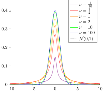
Figure 1: Standard Student-$t$ distribution $T_{\nu}(0,1)$ for different values of $\nu$ in comparison with the standard normal distribution $\mathcal{N}(0,1)$.

The construction of MMs arises from the following scenario: we have $K$ random number generators sampling from different distributions. Now we first choose one of the random number generators randomly using the probability weights $\alpha=(\alpha_{1},...,\alpha_{K})\in\Delta_{K}$ and sample from the corresponding distribution. If all random number generators sample from Student-$t$ distributions we arrive at Student-$t$ MMs. More precisely, if $Y$ is a random variable mapping into $\{1,...,K\}$ and $X_{1},...,X_{k}$ are random variables with $X_{k}\sim T_{\nu_{k}}(\mu_{k},\Sigma_{k})$, then the random variable $X_{Y}$ is a Student-$t$ MM with probability density function

$$p(x)=\sum_{k=1}^{K}\alpha_{k}f(x|\nu_{k},\mu_{k},\Sigma_{k}),\qquad\alpha\in\Delta_{K}.$$ (157)

For samples $\mathcal{X}=(x_{1},...,x_{n})$, we aim to find the parameters of the the Student-$t$ MM by minimizing its negative log-likelihood function

$$\mathcal{L}(\alpha,\nu,\mu,\Sigma|\mathcal{X})=-\frac{1}{n}\sum_{i=1}^{n}\log\bigg{(}\sum_{k=1}^{K}\alpha_{k}f(x_{i}|\nu_{k},\mu_{k},\Sigma_{k})\bigg{)}$$ (158)

subject to the parameter constraints. A first idea to rewrite this problem in the form (3) looks as

$$F(\alpha,\nu,\mu,\Sigma)=H(\alpha,\nu,\mu,\Sigma)+f_{1}(\alpha)+f_{2}(\nu)+f_{3}(\mu)+f_{4}(\Sigma),$$ (159)

where $H\coloneqq\mathcal{L}$, $f_{1}\coloneqq\iota_{\Delta_{K}}$, $f_{2}\coloneqq\iota_{\mathbb{R}^{K}_{>0}}$, $f_{3}\coloneqq 0$, $f_{4}\coloneqq\iota_{\operatorname{SPD}(d)^{K}}$, and $\iota_{\mathcal{S}}$ denotes the indicator function of the set ${\mathcal{S}}$ defined by $\iota_{\mathcal{S}}(x)\coloneqq 0$ if $x\in\mathcal{S}$ and $\iota_{\mathcal{S}}(x)\coloneqq\infty$ otherwise. Indeed one of the authors has applied PALM and iPALM to such a setting without any convergence guarantee in [20]. The problem is that $\mathcal{L}$ is not defined on the whole Euclidean space and since $\mathcal{L}(\alpha,\nu,\mu,\Sigma)\to\infty$ if $\Sigma_{k}\to 0$ for some $k$, the function can also not continuously extended to the whole $\mathbb{R}^{K}\times\mathbb{R}^{K}\times\mathbb{R}^{d\times K}\times\operatorname{Sym}(d)^{K}$. Furthermore, the functions $f_{2}$ and $f_{4}$ are not lower semi-continuous. Consequently, the function (159) does not fulfill the assumptions required for the convergence of PALM and iPALM as well as their stochastic variants. Therefore we modify the above model as follows: Let $\operatorname{SPD}_{\epsilon}(d)\coloneqq\{\Sigma\in\operatorname{SPD}(d):\Sigma\succeq\epsilon I_{d}\}$. Then we use the surjective mappings $\varphi_{1}\colon\mathbb{R}^{K}\to\Delta_{K}$, $\varphi_{2}\colon\mathbb{R}^{K}\to\mathbb{R}_{\geq\epsilon}^{K}$ and $\varphi_{3}\colon\mathrm{Sym}(d)^{K}\to\operatorname{SPD}_{\varepsilon}(d)^{K}$ defined by

$$\varphi_{1}(\alpha)\coloneqq\frac{\exp(\alpha)}{\sum_{j=1}^{K}\exp(\alpha_{j})},\quad\varphi_{2}(\nu)\coloneqq\nu^{2}+\epsilon,\quad\varphi_{3}(\Sigma)\coloneqq\left(\Sigma_{k}^{T}\Sigma_{k}+\epsilon I_{d}\right)_{k=1}^{K}$$ (160)

to reshape problem (159) as the unconstrained optimization problem

$$\operatorname*{argmin}_{\alpha\in\mathbb{R}^{K},\nu\in\mathbb{R}^{K},\mu\in\mathbb{R}^{d\times K},\Sigma\in\operatorname{Sym}(d)^{K}}H(\alpha,\nu,\mu,\Sigma)\coloneqq{\mathcal{L}}(\varphi_{1}(\alpha),\varphi_{2}(\nu),\mu,\varphi_{3}(\Sigma)|\mathcal{X}).$$ (161)

Note that the functions $f_{i}$, $i=1,\ldots,4$ are just zero.

For problem (161), PALM and iPALM reduce basically to block gradient descent algorithms as in Algorithm 1 and 2, respectively. Note that we use $\beta_{i}^{k}=0$ for all $k,i$ and $\alpha_{i}^{k}=\rho^{k}$ for $i=1,\ldots,4$ as iPALM parameters in Algorithm 2. For the stochastic variants SPRING and iSPALM, we have just to replace the gradient by a stochastic gradient estimator.

Algorithm 1 Proximal Alternating Linearized Minimization (PALM) for Student-$t$ MMs

Input: $x_{1},\ldots,x_{n}\in\mathbb{R}^{d}$, $\alpha^{0}\in\mathbb{R}^{K}$, $\nu^{0}\in\mathbb{R}^{K}$, $\mu^{0}\in\mathbb{R}^{d\times K}$, $\Sigma^{0}\in\mathbb{R}^{d\times d\times K}$, $\tau_{1}^{k},\tau_{2}^{k},\tau_{3}^{k},\tau_{4}^{k}$ for $k\in\mathbb{N}$

for $k=1,...$ do

     $\alpha$-Update:

     $\alpha^{k+1}=\alpha^{k}-\frac{1}{\tau_{1}^{k}}\nabla_{\alpha}H(\alpha^{k},\nu^{k},\mu^{k},\Sigma^{k})$

     $\nu$-Update:

     $\nu^{k+1}=\nu^{k}-\frac{1}{\tau_{2}^{k}}\nabla_{\nu}H(\alpha^{k+1},\nu^{k},\mu^{k},\Sigma^{k})$

     $\mu$-Update:

     $\mu^{k+1}=\mu^{k}-\frac{1}{\tau_{3}^{k}}\nabla_{\mu}H(\alpha^{k+1},\nu^{k+1},\mu^{k},\Sigma^{k})$

     $\Sigma$-Update:

     $\Sigma^{k+1}=\Sigma^{k}-\frac{1}{\tau_{4}^{k}}\nabla_{\Sigma}H(\alpha^{k+1},\nu^{k},\mu^{k+1},\Sigma^{k})$

Algorithm 2 Inertial Proximal Alternating Linearized Minimization (iPALM) for Student-$t$ MMs

Input: $x_{1},\ldots,x_{n}\in\mathbb{R}^{d}$, $\alpha^{0}\in\mathbb{R}^{K}$, $\nu^{0}\in\mathbb{R}^{K}$, $\mu^{0}\in\mathbb{R}^{d\times K}$, $\Sigma^{0}\in\mathbb{R}^{d\times d\times K}$, $\rho^{k}\in[0,1]$, $\tau_{1}^{k},\tau_{2}^{k},\tau_{3}^{k},\tau_{4}^{k}$ for $k\in\mathbb{N}$

for $k=1,...$ do

     $\alpha$-Update:

     $\alpha_{z}^{k}=\alpha^{k}+\rho^{k}(\alpha^{k}-\alpha^{k-1})$

     $\alpha^{k+1}=\alpha_{z}^{k}-\frac{1}{\tau_{1}^{k}}\nabla_{\alpha}H(\alpha_{z}^{k},\nu^{k},\mu^{k},\Sigma^{k})$

     $\nu$-Update:

     $\nu_{z}^{k}=\nu^{k}+\rho^{k}(\nu^{k}-\nu^{k-1})$

     $\nu^{k+1}=\nu_{z}^{k}-\frac{1}{\tau_{2}^{k}}\nabla_{\tilde{\nu}}H(\alpha^{k+1},\nu_{z}^{k},\mu^{k},\Sigma^{k})$

     $\mu$-Update:

     $\mu_{z}^{k}=\mu^{k}+\rho^{k}(\mu^{k}-\mu^{k-1})$

     $\mu^{k+1}=\mu_{z}^{k}-\frac{1}{\tau_{3}^{k}}\nabla_{\mu}H(\alpha^{k+1},\nu^{k+1},\mu_{z}^{k},\Sigma^{k})$

     $\Sigma$-Update:

     $\Sigma_{z}^{k}=\Sigma^{k}+\rho^{k}(\Sigma^{k}-\Sigma^{k-1})$

     $\Sigma^{k+1}=\Sigma_{z}^{k}-\frac{1}{\tau_{4}^{k}}\nabla_{\Sigma}H(\alpha^{k+1},\nu^{k+1},\mu^{k+1},\Sigma_{z}^{k})$

Finally, we will show that $H$ in (161)

• is a KL function which is bounded from below, and

• satisfies the Assumption 3.1(i).

Since $H\in C^{2}(\mathbb{R}^{K}\times\mathbb{R}^{K}\times\mathbb{R}^{d\times K}\times\operatorname{Sym}(d)^{K})$ we know by Remark 3.2 that Assumption 3.1(ii) is also fulfilled. Further, $\nabla H$ is continuous on bounded sets. Then, choosing the parameters of PALM, resp. iPALM as required by Theorem 3.3 resp. 3.6, we conclude that the sequences generated by both algorithms converge to a critical point of $H$ supposed that they are bounded. Similarly, if we assume in addition that the stochastic gradient estimators are variance-reduced, resp. inertial variance-reduced, we can conclude that the sequences of SPRING and iSPALM converge as in Theorem 4.4 resp. Theorems 5.5 and 5.6, if the corresponding requirements on the parameters are fulfilled.

We start with the KL property.

Lemma 6.1.

The function $H:\mathbb{R}^{K}\times\mathbb{R}^{K}\times\mathbb{R}^{d\times K}\times\operatorname{Sym}(d)^{K}\to\mathbb{R}$ defined in (161) is a KL function. Moreover, it is bounded from below.

Proof.

1. Since the Gamma function is real analytic, we have that $H$ is a combination of sums, products, quotients and concatenations of real analytic functions. Thus $H$ is real analytic. This implies that it is a KL function, see [1, Example 1] and [28, 29].

2. First, we proof that $f(x|\nu,\mu,\Sigma)$ is bounded from above for $\nu>\epsilon,\mu\in\mathbb{R}^{d}$ and $\Sigma\succeq\epsilon I_{d}$. By definition of the Gamma function and since

$$\Gamma(\tfrac{\nu+d}{2})/\Gamma(\tfrac{\nu}{2})\nu^{\tfrac{d}{2}}\to 1\quad\text{as}\quad\nu\to\infty$$ (162)

we have that (162) is bounded from below for $\nu\in[\epsilon,\infty)$. Further, we see by assumptions on $\nu$ and $\Sigma$ that $\left|\Sigma\right|^{-\tfrac{1}{2}}\leq\epsilon^{-\tfrac{d}{2}}$ and $\left(1+\tfrac{1}{\nu}(x-\mu)^{\mbox{\tiny{T}}}\Sigma^{-1}(x-\mu)\right)^{-\tfrac{d+\nu}{2}}\leq 1$. Thus, $f(x|\nu,\mu,\Sigma)$ is the product of bounded functions and therefore itself bounded by some $C>0$. This yields for $\tilde{\alpha}=\varphi_{1}(\alpha)$, $\tilde{\nu}=\varphi_{2}(\nu)$ and $\tilde{\Sigma}=\varphi_{3}(\Sigma)$ that

$$-\sum_{i=1}^{n}\log\Big{(}\sum_{k=1}^{K}\tilde{\alpha}_{k}f(x_{i}|\tilde{\nu}_{k},\tilde{\mu}_{k},\tilde{\Sigma}_{k})\Big{)}\leq-\sum_{i=1}^{n}\log\Big{(}\sum_{k=1}^{K}\tilde{\alpha}_{k}C\Big{)}\leq-n\log C,$$

which finishes the proof. ∎

Here are the Lipschitz properties of $H$.

Lemma 6.2.

For $H:\mathbb{R}^{K}\times\mathbb{R}^{K}\times\mathbb{R}^{d\times K}\times\operatorname{Sym}(d)^{K}\to\mathbb{R}$ defined by (161) and all $\alpha\in\mathbb{R}^{K}$, $\nu\in\mathbb{R}^{K}$, $\mu\in\mathbb{R}^{d\times K}$ and $\Sigma\in\mathbb{R}^{d\times d\times K}$ we have that the gradients $\nabla_{\alpha}H(\cdot,\nu,\mu,\Sigma)$, $\nabla_{\nu}H(\alpha,\cdot,\mu,\Sigma)$, $\nabla_{\mu}H(\alpha,\nu,\cdot,\Sigma)$, and $\nabla_{\Sigma}H(\alpha,\nu,\mu,\cdot)$ are globally Lipschitz continuous.

The technical proof of the lemma is given in Appendix D.

7 Numerical Results

In this section, we apply iSPALM with SARAH gradient estimator (iSPALM-SARAH) for two different applications and compare it with PALM, iPALM and SPRING-SARAH. We found numerically, that it increases the stability of SPRING-SARAH and iSPALM-SARAH if we enforce the evaluation of the full gradient at the beginning of each epoch. We run all our experiments on a Lenovo ThinkStation with Intel i7-8700 processor, 32GB RAM and a NVIDIA GeForce GTX 2060 Super GPU. For the implementation we use Python and Tensorflow.

7.1 Parameter Choice and Implementation Aspects

On the one hand, the algorithms based on PALM have many parameters which enables a high adaptivity of the algorithms to the specific problems. On the other hand, it is often hard to fit these parameters to ensure the optimal performance of the algorithms.

Based on approximations $\tilde{L}_{1}(x_{2}^{k})$ and $\tilde{L}_{2}(x_{1}^{k+1})$ of the partial Lipschitz constants $L_{1}(x_{2}^{k})$ and $L_{2}(x_{1}^{k+1})$ outlined below, we use the following step size parameters $\tau_{i}^{k}$, $i=1,2$:

• For PALM and iPALM, we choose $\tau_{1}^{k}=\tilde{L}_{1}(x_{1}^{k},x_{2}^{k})$ and $\tau_{2}^{k}=\tilde{L}_{2}(x_{1}^{k+1},x_{2}^{k})$ which was also suggested in [4, 37].

• For SPRING-SARAH and iSPALM-SARAH, we choose $\tau_{1}^{k}=s_{1}\tilde{L}_{1}(x_{1}^{k},x_{2}^{k})$ and $\tau_{2}^{k}=s_{1}\tilde{L}_{2}(x_{1}^{k+1},x_{2}^{k})$, where the manually chosen scalar $s_{1}>0$ depends on the application. Note that the authors in [14] propose to take $s_{1}=2$ which was not optimal in our examples.

Computation of Gradients and Approximative Lipschitz Constants

Since the global and partial Lipschitz constants of $H$ are usually unknown, we estimate them locally using the second order derivative of $H$ which exists in our examples. If $H$ acts on a high dimensional space, it is often computationally to costly to compute the full Hessian matrix. Thus we compute a local Lipschitz constant only in the gradient direction, i.e. we compute

$$\tilde{L}_{i}(x_{1},x_{2})\coloneqq\|\nabla_{x_{i}}^{2}H(x_{1},x_{2})g\|,\quad g\coloneqq\frac{\nabla_{x_{i}}H(x_{1},x_{2})}{\|\nabla_{x_{i}}H(x_{1},x_{2})\|}$$ (163)

For the stochastic algorithms we replace $H$ by the approximated function $\tilde{H}(x_{1},x_{2})\coloneqq\tfrac{1}{b}\sum_{i\in B_{i}^{k}}h_{i}(x_{1},x_{2})$, where $B_{i}^{k}$ is the current mini-batch. The analytical computation of $\tilde{L}_{i}$ in (163) is still hard. Even computing the gradient of a complicated function $H$ can be error prone and laborious. Therefore, we compute the (partial) gradients of $H$ or $\tilde{H}$, respectively, using the reverse mode of algorithmic differentiation (also called backpropagation), see e.g. [17]. To this end, note that the chain rule yields that

$$\left\|\nabla_{x_{i}}\left(\|\nabla_{x_{i}}H(x_{1},x_{2})\|^{2}\right)\right\| =\left\|2\|\nabla_{x_{i}}H(x_{1},x_{2})\|\nabla_{x_{i}}^{2}H(x_{1},x_{2})\nabla_{x_{i}}H(x_{1},x_{2})\right\|$$ (164)

$$=2\|\nabla_{x_{i}}H(x_{1},x_{2})\|^{2}\tilde{L}_{i}(x_{1},x_{2}).$$ (165)

Thus, we can compute $\tilde{L}_{i}(x_{1},x_{2})$ by applying two times the reverse mode. If we neglect the taping, the execution time of this procedure can provably be bounded by a constant times the execution time of $H$, see [17, Section 5.4]. Therefore, this procedure gives us an accurate and computationally very efficient estimation of the local partial Lipschitz constant.

Inertial Parameters

For the iPALM and iSPALM-SARAH we have to choose the inertial parameters $\alpha_{i}^{k}\geq 0$ and $\beta_{i}^{k}\geq 0$. With respect to our convergence results we have to assume that there exist $\alpha_{i}^{k}\leq\bar{\alpha}_{i}<\tfrac{1}{2}$ and $\beta_{i}^{k}\leq\bar{\beta}_{i}<1$, $i=1,2$. Note that for convex functions $f$ and $g$, the authors in [37] proved that the assumption on the $\alpha$’s can be lowered to $\alpha_{i}^{k}\leq\bar{\alpha}_{i}<1$ and suggested to use $\alpha_{i}^{k}=\beta_{i}^{k}=\frac{k-1}{k+2}$. Unfortunately, we cannot show this for iSPALM and indeed we observe instability and divergence in iSPALM-SARAH, if we choose $\alpha_{i}^{k}>\frac{1}{2}$. Therefore, we choose for iSPALM-SARAH the parameters

$$\alpha_{i}^{k}=\beta_{i}^{k}=s_{2}\frac{k-1}{k+2},$$ (166)

where the scalar $0<s_{2}<1$ is manually chosen depending on the application.

Implementation

We provide a general framework for implementing PALM, iPALM, SPRING-SARAH and iSPALM-SARAH on a GPU. Using this framework, it suffice to provide an implementation for the functions $H$ and $\mathrm{prox}_{\tau_{i}}^{f_{i}}$ in order to use one of the above algorithms for the function $F(x_{1},...,x_{K})=H(x_{1},...,x_{K})+\sum_{i=1}^{K}f_{i}(x_{i})$. We provide also the code of our numerical examples below on this website.

7.2 Student-$t$ Mixture Models

We estimate the parameters of the Student-$t$ MM (161) with $K$ components and data points $\mathcal{X}=(x_{1},...,x_{n})\in\mathbb{R}^{d\times n}$. We generate the data by sampling from a Student-$t$ MM as described above. The parameters of the ground truth MM are generate as follows:

• We generate $\alpha=\frac{\bar{\alpha}^{2}+1}{\|\bar{\alpha}^{2}+1\|_{1}}$, where the entries of $\bar{\alpha}\in\mathbb{R}^{K}$ are drawn independently from the standard normal distribution.

• We generate $\nu_{i}=\min(\bar{\nu}_{i}^{2}+1,100)$, where $\bar{\nu}_{i}$, $i=1,\ldots,n$ is drawn from a normal distribution with mean $0$ and standard deviation $10$.

• The entries of $\mu\in\mathbb{R}^{d\times K}$ are drawn independently from a normal distribution with mean $0$ and standard deviation $2$.

• We generate $\Sigma_{i}=\bar{\Sigma}_{i}^{T}\bar{\Sigma}_{i}+I$, where the entries of $\bar{\Sigma}_{i}\in\mathbb{R}^{d\times d}$ are drawn independently from the standard normal distribution.

For the initialization of the algorithms, we assign to each sample $x_{i}$ randomly a class $c_{i}\in\{1,...,K\}$. Then we initialize the parameters $(\nu_{k},\mu_{k},\Sigma_{k})$ by estimating the parameters of a Student-t distribution of all samples with $c_{i}=k$ using a faster alternative of the EM algorithm called multivariate myriad filter, see [18]. Further we initialize $\alpha$ by $\alpha_{k}=\frac{|\{i\in\{1,...,N\}:c_{i}=k\}|}{N}$. We run the algorithm for $n=200000$ data points of dimension $d=10$ and $K=30$ components. We use a batch size of $b=20000$. To represent the randomness in SPRING-SARAH and iSPALM-SARAH, we repeat the experiment $100$ times with the same samples and the same initialization. The resulting mean and standard deviation of the negative log-likelihood values versus the number of epochs and the execution times, respectively, are given in Figure 2. Further, we visualize the mean squared norm of the gradient after each epoch. One epoch contains for SPRING-SARAH and iSPALM-SARAH $10$ steps and for PALM and iPALM $1$ step. We see that in terms of the number of epochs as well as in terms of the execution time the iSPALM-SARAH is the fastest algorithm.

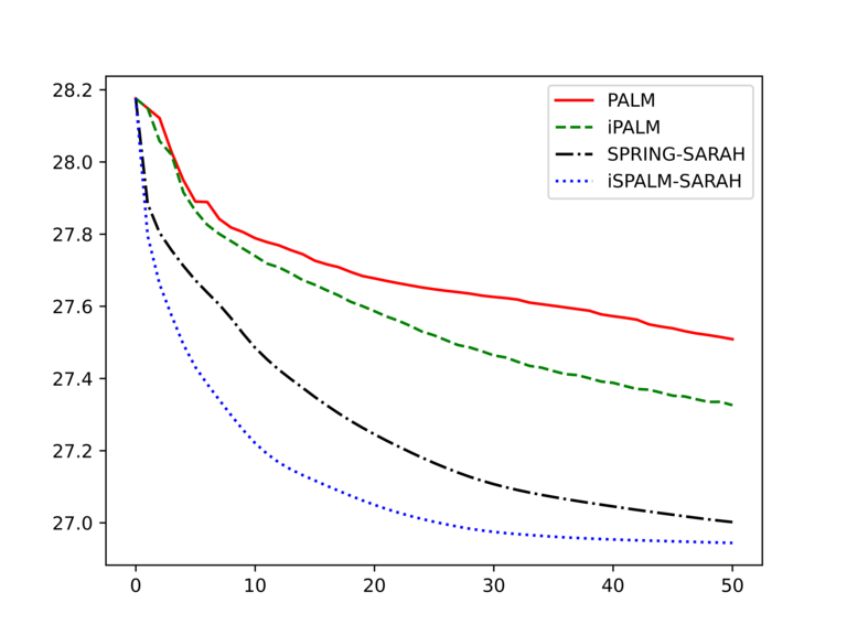
(a) Average objective versus epochs

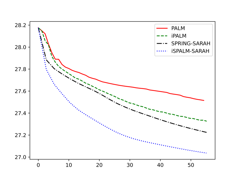
(b) Average objective versus execution time

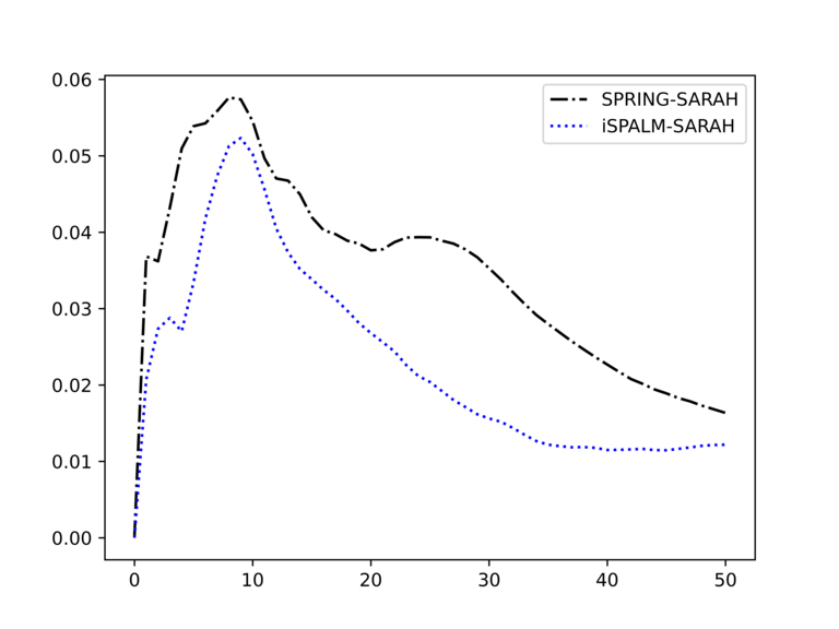
(c) Standard deviation of the objective versus epochs

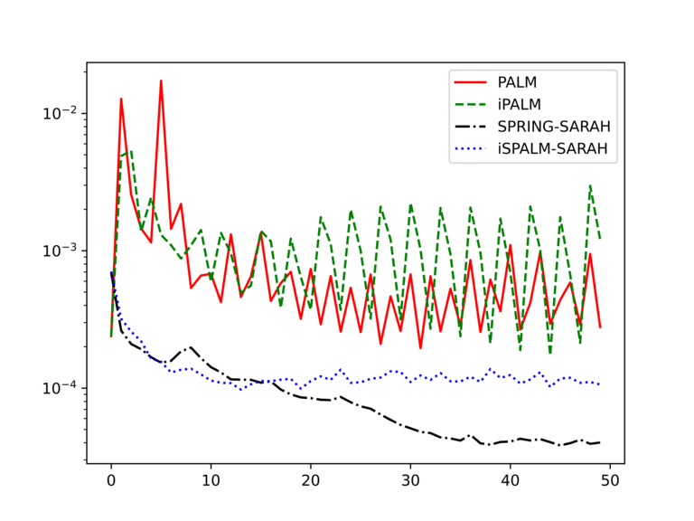
(d) Average squared norm of the gradient versus epochs

Figure 2: Objective function versus number of epochs and versus execution time for estimating the parameters of Student-$t$ MMs

7.3 Proximal Neural Networks (PNNs)

PNNs for MNIST classification

In this example, we train a Proximal Neural Network as introduced in [19] for classification on the MNIST data set. The training data consists of $N=60000$ images $x_{i}\in\mathbb{R}^{d}$ of size $d=28^{2}$ and labels $y_{i}\in\{0,1\}^{10}$, where the $j$th entry of $y_{i}$ is $1$ if and only if $x_{i}$ has the label $j$. A PNN with $K-1$ layers and activation function $\sigma$ is defined by

$$T_{K-1}^{\mbox{\tiny{T}}}\sigma(T_{K-1}...T_{1}^{\mbox{\tiny{T}}}\sigma(T_{1}x+b_{1})...+b_{K-1}),$$

where the $T_{i}$ are contained in the (compact) Stiefel manifold $\,\mathrm{St}(d,n_{i})$ and $b_{i}\in\mathbb{R}^{n_{i}}$ for $i=1,...,K-1$. To get $10$ output elements in $(0,1)$, we add similar as in [19] an additional layer

$$g(T_{K}x),\quad T_{K}\in[-10,10]^{10,d},b_{K}\in\mathbb{R}^{10}$$

with the activation function $g(x)\coloneqq\tfrac{1}{1+\exp(-x)}$. Thus the full network is given by

$$\Psi(x,u)=g(T_{K}T_{K-1}^{\mbox{\tiny{T}}}\sigma(T_{K-1}...T_{1}^{\mbox{\tiny{T}}}\sigma(T_{1}x+b_{1})+...+b_{K-1})+b_{K}),\quad u=(T_{1},...,T_{K},b_{1},...,b_{K}).$$

It was demonstrated in [19] that this kind of network is more stable under adversarial attacks than the same network without the orthogonality constraints.

Training PNNs with iSPALM-SARAH

Now, we want to train a PNN with $K-1=3$ layers and $n_{1}=784$, $n_{2}=400$ and $n_{3}=200$ for MNIST classification. In order of applying our theory, we use the exponential linear unit (ELU)

$$\sigma(x)=\begin{cases}\exp(x)-1,&$if $x<0,\\ x&$if $x\geq 0,\end{cases}$$

as activation function, which is differentiable with a $1$-Lipschitz gradient. Then, the loss function is given by

$$F(u)=H(u)+f(u),\quad u=(T_{1},...,T_{4},b_{1},...,b_{4})$$

where $T_{i}\in\mathbb{R}^{d,n_{i}}$, $b_{i}\in\mathbb{R}^{n_{i}}$, $i=1,2,3$, and $T_{4}\in[-10,10]^{10,d}$, $b_{4}\in\mathbb{R}^{10}$, and $f(u)=\iota_{\mathcal{U}}$ with

$$\mathcal{U}\coloneqq\{(T_{1},...,T_{4},b_{1},...,b_{4}):T_{i}\in\,\mathrm{St}(d,n_{i}),i=1,2,3,T_{4}\in[-10,10]^{10,d}\}.$$

and

$$H(u)\coloneqq\frac{1}{N}\sum_{i=1}^{N}\|\Psi(x_{i},u)-y_{i}\|^{2}.$$

Since $H$ is unfortunately not Lipschitz continuous, we propose a slight modification. Note that for any $u=(T_{1},...,T_{4},b_{1},...,b_{4})$ which appears as $x^{k}$, $y^{k}$ or $z^{k}$ in PALM, iPALM, SPRING-SARAH or iSPALM-SARAH we have that there exist $v,w\in\mathcal{U}$ such that $u=v+w$. In particular, we have that $\|T_{i}\|_{F}\leq 2\sqrt{d}$, $i=1,2,3$ and $\|T_{4}\|_{F}\leq 20\sqrt{10d}$ Therefore, we can replace $H$ by

$$\tilde{H}(u)=\Pi_{i=1}^{4}\eta(\|T_{i}\|_{F}^{2})\frac{1}{N}\sum_{i=1}^{N}\|\Psi(x_{i},u)-y_{i}\|^{2},$$

without changing the algorithm, where $\eta$ is a smooth cutoff function of the interval $(-\infty,4000d]$. Now, simple calculations yield that the function $\tilde{H}$ is globally Lipschitz continuous. Since it is also bounded from below by $0$ we can conclude that our convergence results of iSPALM-SARAH are applicable.

Remark 7.1.

For the implementation, we need to calculate $\mathrm{prox}_{\tilde{f}}$, which is the orthogonal projection $P_{\mathcal{U}}$ onto $\mathcal{U}$. This includes the projection of the matrices $T_{i}$, $i=1,2,3$ onto the Stiefel manifold. In [23, Section 7.3,7.4] it is shown, that the projection of a matrix $A$ onto the Stiefel manifold is given by the $U$-factor of the polar decomposition $A=US\in\mathbb{R}^{d,n}$, where $U\in\,\mathrm{St}(d,n)$ and $S$ is symmetric and positive definite. Note that $U$ is only unique, if $A$ is non-singular. Several possibilities for the computing $U$ are considered in [22, Chapter 8]. In particular, $U$ is given by $VW$, where $A=V\Sigma W$ is the singular value decomposition of $A$. For our numerical experiments we use the iteration

$$Y_{k+1}=2Y_{k}(I+Y_{k}^{\mbox{\tiny{T}}}Y_{k})^{-1}$$

with $Y_{0}=A$, which converges for any non-singular $A$ to $U$, see [22]. $\Box$

Now we run PALM, iPALM, SPRING-SARAH and iSPRING-SARAH algorithms for $200$ epochs using a batch size of $b=1500$. One epoch contains for SPRING-SARAH and iSPALM-SARAH $40$ steps and for PALM and iPALM $1$ step. We repeat the experiment 10 times with the same initialization and plot for the resulting loss functions mean and standard deviation to represent the randomness of the algorihtms. Figure 3 shows the mean and standard deviation of the loss versus the number of epochs or the execution time as well as the squared norm of the Riemannian gradient for the iterates of iSPALM-SARAH after each epoch. We observe that iSPALM-SARAH performs much better than SPRING-SARAH and that iPALM performs much better than PALM. Therefore this example demonstrates the importance of the inertial parameters in iPALM and iSPALM-SARAH. Further, iSPALM-SARAH and SPRING-SARAH outperform their deterministic versions significantly. The resulting weights from iSPALM-SARAH reach after $200$ epochs an average accuracy of $0.985$ on the test set.

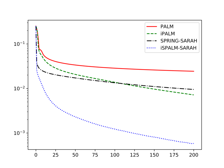
(a) Average loss versus epochs on the training set.

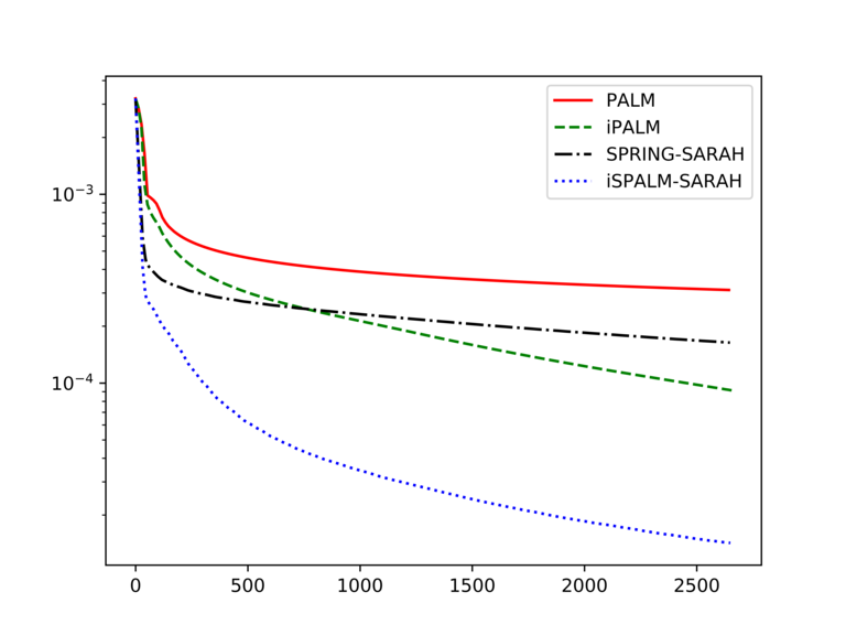
(b) Average loss versus execution time on the training set.

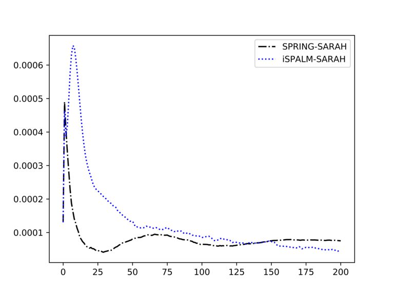
(c) Standard deviation of the loss versus execution time on the training set.

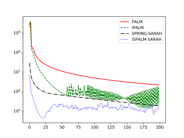
(d) Riemannian gradient of the loss versus epochs on the training set.

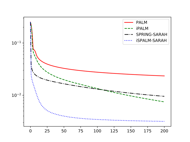
(e) Average loss versus epochs on the test set.

(f) Average loss versus execution time on the test set.

Figure 3: Loss function versus number of epochs and versus execution time for training a PNN for MNIST classification.

8 Conclusions

We combined a stochastic variant of the PALM algorithm with the inertial PALM algorithm to a new algorithm, called iSPALM. We analyzed the convergence behavior of iSPALM and proved convergence results, if the gradient estimators is inertial variance-reduced. In particular, we showed that the expected distance of the subdifferential to zero converges to zero for the sequence of iterates generated by iSPALM. Additionally the sequence of function values achieves linear convergence for functions satisfying a global error bound. We proved that a modified version of the negative log-likelihood function of Student-$t$ MMs fulfills all necessary convergence assumption of PALM, iPALM. We demonstrated the performance of iSPALM for two quite different applications. In the numerical comparison, it turns out that iSPALM shows the best performance of all four algorithms. In particular, the example with the PNNs demonstrates the importance of combining inertial parameters and stochastic gradient estimators for learning applications.

For future work, it would be interesting to compare the performance of the iSPALM algorithm with more classical algorithms for estimating the parameters of Student-$t$ MMs, in particular with the EM algorithm and some of its accelerations. For first experiments in this direction we refer to our work [18, 20].

Further, Driggs et al. [14] proved tighter convergence rates for SPRING if the objective function is semi-algebraic. Whether these convergence rates also hold true for iSPALM is still open.

Finally, we intend to apply iSPALM to other practical problems as e.g. in more sophisticated examples of deep learning.

Appendix A KL Functions

Finally, let us recall the notation of Kurdyka-Łojasiewicz functions. For $\eta\in(0,\infty]$, we denote by $\Phi_{\eta}$ the set of all concave continuous functions $\phi\colon[0,\eta)\to\mathbb{R}_{\geq 0}$ which fulfill the following properties:

1. $\phi(0)=0$.

2. $\phi$ is continuously differentiable on $(0,\eta)$.

3. For all $s\in(0,\eta)$ it holds $\phi^{\prime}(s)>0$.

Definition A.1 (Kurdyka-Łojasiewicz property).

A proper, lower semicontinuous function $\sigma\colon\mathbb{R}^{d}\to(-\infty,+\infty]$ has the Kurdyka-Łojasieweicz (KL) property at $\bar{u}\in\mathrm{dom}\,\partial\sigma=\{u\in\mathbb{R}^{d}:\partial\sigma\neq\emptyset\}$ if there exist $\eta\in(0,\infty]$, a neighborhood $U$ of $\bar{u}$ and a function $\phi\in\Phi_{\eta}$, such that for all

$$u\in U\cap\{v\in\mathbb{R}^{d}:\sigma(\bar{u})<\sigma(v)<\sigma(\bar{u})+\eta\},$$

it holds

$$\phi^{\prime}(\sigma(u)-\sigma(\bar{u}))\,\mathrm{dist}(0,\partial\sigma(u))\geq 1.$$

We say that $\sigma$ is a KL function, if it satisfies the KL property in each point $u\in\mathrm{dom}\,\partial\sigma$.

Appendix B Proof of Proposition 4.8

The proof follows the path of those in [14, Proposition 2.2]. Let $\mathbb{E}_{k,p}=\mathbb{E}(\cdot|(x_{1}^{1},x_{2}^{1}),...,(x_{1}^{k},x_{2}^{k}),p_{1}^{k})$ denote the expectation conditioned on the first $k$ iterations and the event that we do not compute the full gradient at the $k$-th iteration in (32), $k\geq 1$. Then we get

$$\mathbb{E}_{k,p}\left(\tilde{\nabla}_{x_{1}}H(z_{1}^{k},x_{2}^{k})\right) =\tfrac{1}{b}\mathbb{E}_{k,p}\Big{(}\sum_{i\in B_{1}^{k}}\nabla_{x_{1}}h_{i}(z_{1}^{k},x_{2}^{k})-\nabla_{x_{1}}h_{i}(z_{1}^{k-1},x_{2}^{k-1})\Big{)}+\tilde{\nabla}_{x_{1}}H(z_{1}^{k-1},x_{2}^{k-1})$$ (167)

$$=\nabla_{x_{1}}H(z_{1}^{k},x_{2}^{k})-\nabla_{x_{1}}H(z_{1}^{k-1},x_{2}^{k-1})+\tilde{\nabla}_{x_{1}}H(z_{1}^{k-1},x_{2}^{k-1}),$$ (168)

and further

$$\mathbb{E}_{k,p}\left(\|\tilde{\nabla}_{x_{1}}H(z_{1}^{k},x_{2}^{k})-\nabla_{x_{1}}H(z_{1}^{k},x_{2}^{k})\|^{2}\right)$$ (169)

$$=\mathbb{E}_{k,p}\left(\|\tilde{\nabla}_{x_{1}}H(z_{1}^{k-1},x_{2}^{k-1})-\nabla_{x_{1}}H(z_{1}^{k-1},x_{2}^{k-1})+\nabla_{x_{1}}H(z_{1}^{k-1},x_{2}^{k-1})-\nabla_{x_{1}}H(z_{1}^{k},x_{2}^{k})\right.$$ (170)

$$\left.+\tilde{\nabla}_{x_{1}}H(z_{1}^{k},x_{2}^{k})-\tilde{\nabla}_{x_{1}}H(z_{1}^{k-1},x_{2}^{k-1})\|^{2}\right)$$ (171)

$$=\|\tilde{\nabla}_{x_{1}}H(z_{1}^{k-1},x_{2}^{k-1})-\nabla_{x_{1}}H(z_{1}^{k-1},x_{2}^{k-1})\|^{2}+\|\nabla_{x_{1}}H(z_{1}^{k-1},x_{2}^{k-1})-\nabla_{x_{1}}H(z_{1}^{k},x_{2}^{k})\|^{2}$$ (172)

$$+\mathbb{E}_{k,p}\left(\|\tilde{\nabla}_{x_{1}}H(z_{1}^{k},x_{2}^{k})-\tilde{\nabla}_{x_{1}}H(z_{1}^{k-1},x_{2}^{k-1})\|^{2}\right)$$ (173)

$$+2\left\langle\tilde{\nabla}_{x_{1}}H(z_{1}^{k-1},x_{2}^{k-1})-\nabla_{x_{1}}H(z_{1}^{k-1},x_{2}^{k-1}),\nabla_{x_{1}}H(z_{1}^{k-1},x_{2}^{k-1})-\nabla_{x_{1}}H(z_{1}^{k},x_{2}^{k})\right\rangle$$ (174)

$$+2\left\langle\tilde{\nabla}_{x_{1}}H(z_{1}^{k-1},x_{2}^{k-1})-\nabla_{x_{1}}H(z_{1}^{k-1},x_{2}^{k-1}),\mathbb{E}_{k,p}\left(\tilde{\nabla}_{x_{1}}H(z_{1}^{k},x_{2}^{k})-\tilde{\nabla}_{x_{1}}H(z_{1}^{k-1},x_{2}^{k-1})\right)\right\rangle$$ (175)

$$+2\left\langle\nabla_{x_{1}}H(z_{1}^{k-1},x_{2}^{k-1})-\nabla_{x_{1}}H(z_{1}^{k},x_{2}^{k}),\mathbb{E}_{k,p}\left(\tilde{\nabla}_{x_{1}}H(z_{1}^{k},x_{2}^{k})-\tilde{\nabla}_{x_{1}}H(z_{1}^{k-1},x_{2}^{k-1})\right)\right\rangle.$$ (176)

By (168), we see that

$$\mathbb{E}_{k,p}\left(\tilde{\nabla}_{x_{1}}H(z_{1}^{k},x_{2}^{k})-\tilde{\nabla}_{x_{1}}H(z_{1}^{k-1},x_{2}^{k-1})\right)=\nabla_{x_{1}}H(z_{1}^{k},x_{2}^{k})-\nabla_{x_{1}}H(z_{1}^{k-1},x_{2}^{k-1}).$$

Thus, the first two inner products in (176) sum to zero and the third one is equal to

$$2\left\langle\nabla_{x_{1}}H(z_{1}^{k-1},x_{2}^{k-1})-\nabla_{x_{1}}H(z_{1}^{k},x_{2}^{k}),\mathbb{E}_{k,p}\left(\tilde{\nabla}_{x_{1}}H(z_{1}^{k},x_{2}^{k})-\tilde{\nabla}_{x_{1}}H(z_{1}^{k-1},x_{2}^{k-1})\right)\right\rangle$$ (177)

$$=2\left\langle\nabla_{x_{1}}H(z_{1}^{k-1},x_{2}^{k-1})-\nabla_{x_{1}}H(z_{1}^{k},x_{2}^{k}),\nabla_{x_{1}}H(z_{1}^{k},x_{2}^{k})-\nabla_{x_{1}}H(z_{1}^{k-1},x_{2}^{k-1})\right\rangle$$ (178)

$$=-2\|\nabla_{x_{1}}H(z_{1}^{k},x_{2}^{k})-\nabla_{x_{1}}H(z_{1}^{k-1},x_{2}^{k-1})\|^{2}.$$ (179)

This yields

$$\mathbb{E}_{k,p}\left(\|\tilde{\nabla}_{x_{1}}H(z_{1}^{k},x_{2}^{k})-\nabla_{x_{1}}H(z_{1}^{k},x_{2}^{k})\|^{2}\right)$$ (180)

$$\leq\|\tilde{\nabla}_{x_{1}}H(z_{1}^{k-1},x_{2}^{k-1})-\nabla_{x_{1}}H(z_{1}^{k-1},x_{2}^{k-1})\|^{2}-\|\nabla_{x_{1}}H(z_{1}^{k-1},x_{2}^{k-1})-\nabla_{x_{1}}H(z_{1}^{k},x_{2}^{k})\|^{2}$$ (181)

$$+\mathbb{E}_{k,p}\left(\|\tilde{\nabla}_{x_{1}}H(z_{1}^{k},x_{2}^{k})-\tilde{\nabla}_{x_{1}}H(z_{1}^{k-1},x_{2}^{k-1})\|^{2}\right)$$ (182)

$$\leq\|\tilde{\nabla}_{x_{1}}H(z_{1}^{k-1},x_{2}^{k-1})\!-\!\nabla_{x_{1}}H(z_{1}^{k-1},x_{2}^{k-1})\|^{2}+\mathbb{E}_{k,p}\left(\|\tilde{\nabla}_{x_{1}}H(z_{1}^{k},x_{2}^{k})\!-\!\tilde{\nabla}_{x_{1}}H(z_{1}^{k-1},x_{2}^{k-1})\|^{2}\right).$$ (183)

Since the function $x\mapsto\|x\|^{2}$ is convex, the second summand fulfills

$$\mathbb{E}_{k,p}\left(\|\tilde{\nabla}_{x_{1}}H(z_{1}^{k},x_{2}^{k})-\tilde{\nabla}_{x_{1}}H(z_{1}^{k-1},x_{2}^{k-1})\|^{2}\right)$$ (184)

$$=\mathbb{E}_{k,p}\Big{(}\Big{\|}\tfrac{1}{b}\Big{(}\sum_{j\in B_{1}^{k}}\nabla_{x_{1}}h_{j}(z_{1}^{k},x_{2}^{k})-\nabla_{x_{1}}h_{j}(z_{1}^{k-1},x_{2}^{k-1})\Big{)}\Big{\|}^{2}\Big{)}$$ (185)

$$\leq\tfrac{1}{n}\sum_{j=1}^{n}\|\nabla h_{j}(z_{1}^{k},x_{2}^{k})-\nabla_{x_{1}}h_{j}(z_{1}^{k-1},x_{2}^{k-1})\|^{2},$$ (186)

so that we obtain

$$\mathbb{E}_{k,p}\left(\|\tilde{\nabla}_{x_{1}}H(z_{1}^{k},x_{2}^{k})-\nabla_{x_{1}}H(z_{1}^{k},x_{2}^{k})\|^{2}\right) \leq\|\tilde{\nabla}_{x_{1}}H(z_{1}^{k-1},x_{2}^{k-1})-\nabla_{x_{1}}H(z_{1}^{k-1},x_{2}^{k-1})\|^{2}$$ (187)

$$+\tfrac{1}{n}\sum_{j=1}^{n}\|\nabla_{x_{1}}h_{j}(z_{1}^{k},x_{2}^{k})-\nabla_{x_{1}}h_{j}(z_{1}^{k-1},x_{2}^{k-1})\|^{2}.$$ (188)

Since the conditional expectation $\mathbb{E}_{k}$ of $\|\tilde{\nabla}_{x_{1}}H(z_{1}^{k},x_{2}^{k})-\nabla_{x_{1}}H(z_{1}^{k},x_{2}^{k})\|^{2}$ conditioned on the event that the full gradient is computed in (32) is zero, and taking the $M$-Lipschitz continuity of the gradients of the $h_{j}$ into account, we get

$$\mathbb{E}_{k}\left(\|\tilde{\nabla}_{x_{1}}H(z_{1}^{k},x_{2}^{k})-\nabla_{x_{1}}H(z_{1}^{k},x_{2}^{k})\|^{2}\right)$$ (189)

$$\leq(1-\tfrac{1}{p})\Big{(}\|\tilde{\nabla}_{x_{1}}H(z_{1}^{k-1},x_{2}^{k-1})-\nabla_{x_{1}}H(z_{1}^{k-1},x_{2}^{k-1})\|^{2}$$ (190)

$$+\tfrac{1}{n}\sum_{j=1}^{n}\|\nabla_{x_{1}}h_{j}(z_{1}^{k},x_{2}^{k})-\nabla_{x_{1}}h_{j}(z_{1}^{k-1},x_{2}^{k-1})\|^{2}\Big{)}$$ (191)

$$\leq(1-\tfrac{1}{p})\left(\|\tilde{\nabla}_{x_{1}}H(z_{1}^{k-1},x_{2}^{k-1})-\nabla_{x_{1}}H(z_{1}^{k-1},x_{2}^{k-1})\|^{2}+M^{2}\|(z_{1}^{k},x_{2}^{k})-(z_{1}^{k-1},x_{2}^{k-1})\|^{2}\right).$$ (192)

By symmetric arguments, it holds

$$\mathbb{E}_{k}\left(\|\tilde{\nabla}_{x_{2}}H(x_{1}^{k+1},z_{2}^{k})-\nabla_{x_{2}}H(x_{1}^{k+1},z_{2}^{k})\|^{2}\right)$$ (193)

$$\leq (1-\tfrac{1}{p})\left(\|\tilde{\nabla}_{x_{2}}H(x_{1}^{k},z_{2}^{k-1})-\nabla_{x_{2}}H(x_{1}^{k},z_{2}^{k-1})\|^{2}+M^{2}\mathbb{E}_{k}(\|(x_{1}^{k+1},z_{2}^{k})-(x_{1}^{k},z_{2}^{k-1})\|^{2})\right).$$ (194)

Using $(a+b+c)^{2}\leq 3(a^{2}+b^{2}+c^{2})$ and Lemma 4.7, we can estimate

$$\|(z_{1}^{k},x_{2}^{k})-(z_{1}^{k-1},x_{2}^{k-1})\|^{2}\,=\,\|z_{1}^{k}-z_{1}^{k-1}\|^{2}+\|x_{2}^{k}-x_{2}^{k-1}\|^{2}$$ (195)

$$\leq 3\|z_{1}^{k}-x_{1}^{k}\|^{2}+3\|x_{1}^{k}-x_{1}^{k-1}\|^{2}+3\|x_{1}^{k-1}-z_{1}^{k-1}\|^{2}+\|x_{2}^{k}-x_{2}^{k-1}\|^{2}$$ (196)

$$\leq 3(1+(\beta_{1}^{k})^{2})\|x_{1}^{k}-x_{1}^{k-1}\|^{2}+3(\beta_{1}^{k-1})^{2}\|x_{1}^{k-1}-x_{1}^{k-2}\|^{2}+\|x_{2}^{k}-x_{2}^{k-1}\|^{2}.$$ (197)

Further, we have

$$\mathbb{E}_{k}(\|(x_{1}^{k+1},z_{2}^{k})-(x_{1}^{k},z_{2}^{k-1})\|^{2})\,=\,\mathbb{E}_{k}(\|x_{1}^{k+1}-x_{1}^{k}\|^{2})+\|z_{2}^{k}-z_{2}^{k-1}\|^{2}$$ (198)

$$\leq\mathbb{E}_{k}(\|x_{1}^{k+1}-x_{1}^{k}\|^{2})+3\|z_{2}^{k}-x_{2}^{k}\|^{2}+3\|x_{2}^{k}-x_{2}^{k-1}\|^{2}+3\|x_{2}^{k-1}-z_{2}^{k-1}\|^{2}$$ (199)

$$\leq\mathbb{E}_{k}(\|x_{1}^{k+1}-x_{1}^{k}\|^{2})+3(1+(\beta_{2}^{k})^{2})\|x_{2}^{k}-x_{2}^{k-1}\|^{2}+3(\beta_{2}^{k-1})^{2}\|x_{2}^{k-1}-x_{2}^{k-2}\|^{2}.$$ (200)

Altogether we obtain for

$$\Upsilon_{k+1}\coloneqq\|\tilde{\nabla}_{x_{1}}H(z_{1}^{k},x_{2}^{k})-\nabla_{x_{1}}H(z_{1}^{k},x_{2}^{k})\|^{2}+\|\tilde{\nabla}_{x_{2}}H(x_{1}^{k+1},z_{2}^{k})-\nabla_{x_{2}}H(x_{1}^{k+1},z_{2}^{k})\|^{2}.$$

that

$$\mathbb{E}_{k}(\Upsilon_{k+1})=\mathbb{E}_{k}\left(\|\tilde{\nabla}_{x_{1}}H(z_{1}^{k},x_{2}^{k})-\nabla_{x_{1}}H(z_{1}^{k},x_{2}^{k})\|^{2}+\|\tilde{\nabla}_{x_{2}}H(x_{1}^{k+1},z_{2}^{k})-\nabla_{x_{2}}H(x_{1}^{k+1},z_{2}^{k})\|^{2}\right)$$ (201)

$$\leq(1-\tfrac{1}{p})\Upsilon_{k}+V_{\Upsilon}(\mathbb{E}_{k}(\|x^{k+1}-x^{k}\|^{2})+\|x^{k}-x^{k-1}\|^{2}+\|x^{k-1}-x^{k-2}\|^{2}),$$ (202)

where $V_{\Upsilon}=3(1-\tfrac{1}{p})M^{2}\left(1+\max((\bar{\beta}_{1})^{2},(\bar{\beta}_{2})^{2})\right)$. This proves the properties (i) and (ii) of Definition 4.6. Taking the full expectation in (202) and iterating, we

$$\mathbb{E}(\Upsilon_{k}) \leq(1-\tfrac{1}{p})^{k-1}\mathbb{E}(\Upsilon_{1})$$ (203)

$$+V_{\Upsilon}\sum_{l=1}^{k-1}(1-\tfrac{1}{p})^{k-l-1}\mathbb{E}\left(\|x^{l+1}-x^{l}\|^{2}+\|x^{l}-x^{l-1}\|^{2}+\|x^{l-1}-x^{l-2}\|^{2}\right).$$ (204)

We want to show that $\mathbb{E}(\Upsilon_{k})\to 0$ as $k\to\infty$, if $\mathbb{E}(\|x^{k}-x^{k-1}\|^{2})\to 0$ as $k\to\infty$. Since the first summand converges to zero for $k$ large enough, it remains to prove that for an arbitrary $\epsilon>0$, there exists some $k_{0}\in\mathbb{N}$ such that for all $k\geq k_{0}$ the sum becomes not larger than $\epsilon$ Recall that $\sum_{l=0}^{\infty}(1-\tfrac{1}{p})^{l}=p$. Now we choose $k_{1}\in\mathbb{N}$ such that for all $k\geq k_{1}$ we have $\mathbb{E}(\|x^{k+1}-x^{k}\|^{2})<\tfrac{\epsilon}{2p}$. Further we define $k_{2}\in\mathbb{N}$ such that $(1-\tfrac{1}{p})^{k_{2}}<\tfrac{\epsilon}{6Sp}$, where $S\coloneqq\max_{k\in\mathbb{N}}\mathbb{E}(\|x^{k}-x^{k-1}\|^{2})$. Then the above sum can be estimated for $k\geq k_{0}\coloneqq k_{1}+k_{2}$ as

$$\sum_{l=1}^{k-1}(1-\tfrac{1}{p})^{k-l-1}\mathbb{E}\left(\|x^{l+1}-x^{l}\|^{2}+\|x^{l}-x^{l-1}\|^{2}+\|x^{l-1}-x^{l-2}\|^{2}\right)$$ (205)

$$=\sum_{l=1}^{k_{1}}(1-\tfrac{1}{p})^{k-l-1}\mathbb{E}\left(\|x^{l+1}-x^{l}\|^{2}+\|x^{l}-x^{l-1}\|^{2}+\|x^{l-1}-x^{l-2}\|^{2}\right)$$ (206)

$$+\sum_{l=k_{1}+1}^{k-1}(1-\tfrac{1}{p})^{k-l-1}\mathbb{E}\left(\|x^{l+1}-x^{l}\|^{2}+\|x^{l}-x^{l-1}\|^{2}+\|x^{l-1}-x^{l-2}\|^{2}\right)$$ (207)

$$\leq(1-\tfrac{1}{p})^{k-k_{1}}\sum_{l=1}^{k_{1}}(1-\tfrac{1}{p})^{k_{1}-l}\mathbb{E}\left(\|x^{l+1}-x^{l}\|^{2}+\|x^{l}-x^{l-1}\|^{2}+\|x^{l-1}-x^{l-2}\|^{2}\right)$$ (208)

$$+\sum_{l=k_{1}+1}^{k}(1-\tfrac{1}{p})^{k-l-1}\tfrac{\epsilon}{2p}\leq\epsilon,$$ (209)

and we are done.

Appendix C Derivatives of the Likelihood of Student-$t$ MMs

In this section, we compute the outer derivatives of the objective function in (161) which we need in the numerical computations and in the proof of Lemma 6.2. In [18], the derivatives of $g(\nu,\mu,\Sigma)\coloneqq\log(f(x|\nu,\mu,\Sigma)$ were computed as follows:

$$\frac{\partial g}{\partial\mu}(\nu,\mu,\Sigma) =\frac{d+\nu}{\nu+s}\,\Sigma^{-1}(x-\mu),$$ (210)

$$\frac{\partial g}{\partial\Sigma}(\nu,\mu,\Sigma) =\frac{1}{2}\left(\frac{d+\nu}{\nu+s}\,\Sigma^{-1}(x-\mu)(x-\mu)^{\mbox{\tiny{T}}}\Sigma^{-1}-\Sigma^{-1}\right),$$ (211)

$$\frac{\partial g}{\partial\nu}(\nu,\mu,\Sigma) =\frac{1}{2}\left(\psi\left(\frac{\nu+d}{2}\right)-\psi\left(\frac{\nu}{2}\right)-\frac{d-s}{\nu+s}-\log\left(1+\frac{s}{\nu}\right),\right)$$ (212)

where $s\coloneqq(x-\mu)^{\mbox{\tiny{T}}}\Sigma^{-1}(x-\mu)$ and $\Psi$ is the the digamma function defined by

$$\psi(x)\coloneqq\frac{\mathrm{d}}{\mathrm{d}x}\log\left(\Gamma(x)\right)=\frac{\Gamma^{\prime}(x)}{\Gamma(x)}.$$

We use the abbreviations

$$f_{i,k}\coloneqq f(x_{i}|\nu_{k},\mu_{k},\Sigma_{k}),\quad\gamma_{i}\coloneqq\Big{(}\sum_{k=1}^{K}\alpha_{k}f_{i,k}\Big{)}^{-1},\quad s_{i,k}\coloneqq(x_{i}-\mu_{k})^{T}\Sigma_{k}^{-1}(x_{i}-\mu_{k}).$$

Then we obtain for

$$\mathcal{L}(\alpha,\nu,\mu,\Sigma|\mathcal{X})=-\sum_{i=1}^{n}\log\bigg{(}\sum_{k=1}^{K}\alpha_{k}f_{i,k}\bigg{)}$$

that the derivative with respect to $\alpha$ is given by

$$\frac{\partial\mathcal{L}(\alpha,\nu,\mu,\Sigma|\mathcal{X})}{\partial\alpha_{l}}=-\sum_{i=1}^{n}\gamma_{i}f_{i,k}$$ (213)

Using that for $g=\log f$, the relation $g^{\prime}f=f^{\prime}$ holds true, the derivatives with respect to $\mu_{l},\Sigma_{l}$ and $\nu_{l}$ have the form

$$\frac{\partial\mathcal{L}(\alpha,\nu,\mu,\Sigma|\mathcal{X})}{\partial\bullet_{l}}=-\sum_{i=1}^{n}\gamma_{i}\alpha_{l}f_{i,l}\frac{\partial f(\alpha,\nu,\mu,\Sigma|\mathcal{X})}{\partial\bullet_{l}}.$$ (214)

Together with (210) - (212), we obtain

$$\nabla_{\mu_{l}}\mathcal{L}(\alpha,\nu,\mu,\Sigma|\mathcal{X}) =\sum_{i=1}^{n}\gamma_{i}\alpha_{l}f_{i,l}\frac{d+\nu_{l}}{\nu_{l}+s_{i,l}}\,\Sigma_{l}^{-1}(\mu_{l}-x_{i}),$$ (215)

$$\nabla_{\Sigma_{l}}\mathcal{L}(\alpha,\nu,\mu,\Sigma|\mathcal{X}) =\frac{1}{2}\sum_{i=1}^{n}\gamma_{i}\alpha_{l}f_{i,l}\bigg{(}\Sigma_{l}^{-1}-\frac{d+\nu_{l}}{\nu_{l}+s_{i,l}}\,\Sigma^{-1}(x_{i}-\mu_{l})(x_{i}-\mu_{l})^{T}\Sigma^{-1}\bigg{)},$$ (216)

$$\frac{\partial\mathcal{L}(\alpha,\nu,\mu,\Sigma|\mathcal{X})}{\partial\nu_{l}} =\frac{1}{2}\sum_{i=1}^{n}\gamma_{i}\alpha_{l}f_{i,l}\left(\psi\left(\frac{\nu_{l}}{2}\right)-\psi\left(\frac{\nu_{l}+d}{2}\right)+\frac{d-s_{i,l}}{\nu_{l}+s_{i,l}}+\log\left(1+\frac{s_{i,l}}{\nu_{l}}\right)\right).$$ (217)

Appendix D Proof of Lemma 6.2

Since the sum of Lipschitz continuous functions is Lipschitz continuous, it is sufficient to show the claim for the summands of $H$ in (161). Hence we consider only

$$h(\alpha,\nu,\mu,\Sigma)\coloneqq\log\Big{(}\sum_{k=1}^{K}\tilde{\alpha}_{k}f_{k}\Big{)},\qquad f_{k}\coloneqq f(x|\tilde{\nu}_{k},\tilde{\mu}_{k},\tilde{\Sigma}_{k}),$$

where $\tilde{\alpha}=\varphi_{1}(\alpha)$, $\tilde{\nu}=\varphi_{2}(\nu)$, $\tilde{\Sigma}=\varphi_{3}(\Sigma)$ are given by (160). Set

$$\gamma\coloneqq\left(\sum_{k=1}^{K}\tilde{\alpha}_{k}f_{k}\right)^{-1},\quad s_{k}\coloneqq(x-\tilde{\mu}_{k})^{T}\tilde{\Sigma}_{k}^{-1}(x-\tilde{\mu}_{k}).$$

1. By (213) we obtain

$$\frac{\partial h(\alpha,\nu,\mu,\Sigma)}{\partial\alpha_{l}}=\frac{\exp(\alpha_{l})f_{l}}{\sum_{k=1}^{K}\exp(\alpha_{k})f_{k}}-\frac{\exp(\alpha_{l})}{\sum_{k=1}^{K}\exp(\alpha_{k})}$$ (218)

and further for the Hessian of $h$ with respect to $\alpha$,

$$\frac{\partial h(\alpha,\nu,\mu,\Sigma)}{\partial\alpha_{l}\partial\alpha_{j}} =\delta_{j,l}\left(\frac{\exp(\alpha_{l})f_{l}}{\sum_{k=1}^{K}\exp(\alpha_{k})f_{k}}-\frac{\exp(\alpha_{l})}{\sum_{k=1}^{K}\exp(\alpha_{k})}\right)$$ (219)

$$-\frac{\exp(\alpha_{l})\exp(\alpha_{j})f_{l}f_{j}}{\Big{(}\sum_{k=1}^{K}\exp(\alpha_{k})f_{k}\Big{)}^{2}}+\frac{\exp(\alpha_{l})\exp(\alpha_{j})}{\Big{(}\sum_{k=1}^{K}\exp(\alpha_{k})\Big{)}^{2}}.$$ (220)

This is bounded so that $\nabla_{\alpha}h(\cdot,\nu,\mu,\Sigma)$ is globally Lipschitz continuous.

2. Using (212), we get

$$\frac{\partial}{\partial\nu_{l}}h(\alpha,\nu,\mu,\Sigma)=\tilde{\alpha}_{l}\underbrace{\gamma f_{l}}_{g_{1}}\underbrace{\Big{(}\psi\left(\psi\left(\frac{d+\tilde{\nu}_{l}}{2}\right)-\frac{\tilde{\nu}_{l}}{2}\right)-\frac{d-s_{l}}{\tilde{\nu}_{l}+s_{l}}-\log\left(1+\frac{s_{l}}{\tilde{\nu}_{l}}\right)\Big{)}\,\nu_{l}}_{g_{2}}.$$ (221)

We show that the functions $g_{i}$, $i=1,2$ are Lipschitz continuous and bounded. This implies that $\frac{\partial}{\partial\nu_{l}}h(\alpha,\cdot,\mu,\Sigma)$ is Lipschitz continuous. It holds

$$|g_{2}(\nu_{l})|\leq|\nu_{l}|\,|\psi\left(\frac{d+\tilde{\nu}_{l}}{2}\right)-\psi\left(\frac{\tilde{\nu}_{l}}{2}\right)|+|\nu_{l}|\left|\frac{d-s_{l}}{\tilde{\nu}_{l}+s_{l}}\right|+\log\left(1+\frac{s_{l}}{\tilde{\nu}_{l}}\right)^{|\nu_{l}|}.$$ (222)

Using the summation formula

$$\psi(x+1)=\psi(x)+\tfrac{1}{x}$$ (223)

and the fact that the digamma function is monotone increasing we conclude

$$|g_{2}(\nu)| \leq\sum_{r=1}^{\lceil\tfrac{d}{2}\rceil}\frac{|\nu_{l}|}{\tfrac{d+\tilde{\nu}_{l}}{2}-r}+|\nu_{l}|\Big{|}\frac{d-s_{l}}{\tilde{\nu}_{l}+s_{l}}\Big{|}+\log\left(1+\frac{s_{l}}{\tilde{\nu}_{l}}\right)^{|\nu_{l}|}$$ (224)

$$\leq\sum_{r=1}^{\lceil\tfrac{d}{2}\rceil}\frac{|\nu_{l}|}{\tfrac{d+\nu_{l}^{2}+\epsilon}{2}-r}+|\nu_{l}|\Big{|}\frac{d-s_{l}}{\nu_{l}^{2}+\epsilon+s_{l}}\Big{|}+\log\left(1+\frac{s_{l}}{\nu_{l}^{2}}\right)^{|\nu_{l}|}.$$ (225)

Since

$$\lim_{\nu_{l}\to\pm\infty}\log(1+\tfrac{1}{\nu^{2}}s_{l})^{|\nu|}\leq\lim_{\nu_{l}\to\pm\infty}\log\left(1+\tfrac{1}{\nu^{2}}s_{l}\right)^{\nu^{2}}=s_{l}$$ (226)

and $g_{2}$ is continuous we conclude that $g_{2}$ is bounded. Further, it holds

$$g_{2}^{\prime}(\nu_{l}) =\psi\left(\frac{d+\tilde{\nu}_{l}}{2}\right)-\psi\left(\frac{\tilde{\nu}_{l}}{2}\right)-\frac{d-s_{l}}{\tilde{\nu}_{l}+s_{l}}-\log\left(1+\ \frac{s_{l}}{\tilde{\nu}_{l}}\right)$$ (227)

$$+\nu_{l}^{2}\left(\psi^{\prime}\left(\frac{d+\tilde{\nu}_{l}}{2}\right)-\psi^{\prime}\left(\frac{\tilde{\nu}_{l}}{2}\right)\right)+\frac{2(d-s_{l})\nu_{l}}{(\tilde{\nu}_{l}+s_{l})^{2}}+\frac{2s_{l}\nu_{l}}{(\tilde{\nu}_{l}^{2}+s_{l})^{2}+s_{l}(\tilde{\nu}_{l}^{2}+s_{l})}.$$ (228)

Using again (223) and $\psi^{\prime}(x+1)=\psi^{\prime}(x)+\tfrac{1}{x^{2}}$ as well as the fact that the digamma function and its derivatives are monotone increasing we get,

$$\lim_{\nu_{l}\to\pm\infty}|g_{2}^{\prime}(\nu_{l})| \leq\lim_{\nu_{l}\to\pm\infty}\Big{(}\sum_{r=0}^{\lceil\tfrac{d}{2}\rceil}\frac{1}{\tfrac{\tilde{\nu}_{l}}{2}+r}+\sum_{r=0}^{\lceil\tfrac{d}{2}\rceil}\frac{|\nu_{l}|^{2}}{(\tfrac{\tilde{\nu}_{l}}{2}+r)^{2}}\Big{)}=0.$$ (229)

Since $g_{2}^{\prime}(\nu)$ is continuous, this yields that it is bounded which implies that $g_{2}$ is Lipschitz continuous.

The function $g_{1}$ is obviously bounded. Further we obtain for $j\not=l$ that

$$\nabla_{\nu_{j}}g_{1}(\nu)=-2\tilde{\alpha}_{j}f_{l}\gamma^{2}\frac{\partial f_{j}}{\partial\nu_{j}}=-2g_{2}(\nu_{j})\tilde{\alpha}_{j}f_{l}f_{j}\gamma^{2}$$ (230)

so that

$$|\nabla_{\nu_{j}}g_{1}(\nu_{l})|=2|g_{2}(\nu_{j})|\,|\tilde{\alpha}_{j}f_{l}f_{j}\gamma^{2}|.$$

This expression is bounded. Similarly, we get for $j=l$ that

$$|\nabla_{\nu_{l}}g_{1}(\nu_{l})|=2|g_{2}(\nu_{l})|\,|\tilde{\alpha}_{l}f_{l}^{2}\gamma^{2}+\gamma f_{l}|.$$ (231)

Thus, $g_{1}$ is Lipschitz continuous.

3. By (215) we obtain

$$\nabla_{\mu_{l}}h(\alpha,\nu,\mu,\Sigma)=\tilde{\alpha}_{l}\underbrace{\gamma f_{l}}_{g_{1}}\underbrace{\frac{d+\tilde{\nu}_{l}}{\tilde{\nu}_{l}+s_{l}}\,\tilde{\Sigma}_{l}^{-1}(x-\mu_{l})}_{g_{2}}.$$ (232)

As in the second part of the proof, it suffices to show that $g_{i}$, $i=1,2$ are bounded and Lipschitz continuous. Calculating the Jacobian

$$\nabla_{\mu_{l}}g_{2}(\mu_{l})=\frac{d+\tilde{\nu}_{l}}{(\tilde{\nu}_{l}+s_{l})^{2}}\tilde{\Sigma}_{l}^{-1}(\mu_{l}-x)(\mu_{l}-x)^{T}\tilde{\Sigma}_{l}^{-1}+\frac{d+\tilde{\nu}_{l}}{\tilde{\nu}_{l}+s_{l}}\tilde{\Sigma}_{l}^{-1}$$ (233)

and taking the Frobenius norm $\|\cdot\|_{F}$, we obtain

$$\|\nabla_{\mu_{l}}g_{2}(\mu_{l})\|_{F} \leq\frac{d+\tilde{\nu}_{l}}{(\tilde{\nu}_{l}+s_{l})^{2}}\|\tilde{\Sigma}_{l}^{-1}(\mu_{l}-x)\|^{2}+\mathrm{const}$$ (234)

$$\leq\frac{d+\tilde{\nu}_{l}}{\left(\frac{\tilde{\nu}_{l}}{\|\tilde{\Sigma}_{l}^{-\frac{1}{2}}(\mu-x)\|}+\|\tilde{\Sigma}_{l}^{-\frac{1}{2}}(\mu-x)\|\right)^{2}}\|\tilde{\Sigma}_{l}^{-1}\|_{F}+\mathrm{const}$$ (235)

$$\leq\frac{d+\tilde{\nu}_{l}}{(2\min(1,\tilde{\nu}_{l}))^{2}}\|\tilde{\Sigma}_{l}^{-1}\|_{F}+\mathrm{const}.$$ (236)

Thus $g_{2}$ is Lipschitz continuous. Since

$$\|g_{2}(\mu_{l})\| \leq\frac{d+\tilde{\nu}_{l}}{\tilde{\nu}_{l}+s_{l}}\|\tilde{\Sigma}_{l}^{-\frac{1}{2}}\|_{F}\|\tilde{\Sigma}_{l}^{-\frac{1}{2}}(\mu_{l}-x)\|$$ (237)

$$=\frac{d+\tilde{\nu}_{l}}{\frac{\tilde{\nu}_{l}}{\|\tilde{\Sigma}_{l}^{-\frac{1}{2}}(\mu_{l}-x)\|}+\|\tilde{\Sigma}_{l}^{-\frac{1}{2}}(\mu_{l}-x)\|}\|\tilde{\Sigma}_{l}^{-\frac{1}{2}}\|\leq\frac{d+\tilde{\nu}_{l}}{2\min(1,\tilde{\nu}_{l})}\|\tilde{\Sigma}_{l}^{-\frac{1}{2}}\|,$$ (238)

$g_{2}$ is bounded.

The function $g_{1}$ is obviously bounded. Further, it holds

$$\|\nabla_{\mu_{j}}g_{1}(\mu)\| =\left\{\begin{array}[]{ll}\|g_{2}(\mu_{l})\|\,|\gamma^{2}f_{l}f_{j}\tilde{\alpha}_{j}|&\mathrm{if}\;j\neq l\\ \|g_{2}(\mu_{l})\|\,|\gamma^{2}f_{l}^{2}\tilde{\alpha}_{l}+\gamma f_{l}|&\mathrm{if}\;j=l,\end{array}\right.$$ (241)

so that $g_{1}$ is Lipschitz continuous.

4. At the end, we use (211) to compute

$$\nabla_{\Sigma_{l}}h(\alpha,\nu,\mu,\Sigma)=\tilde{\alpha}_{l}\underbrace{\gamma f_{l}}_{g_{1}}\underbrace{\left(\frac{d+\tilde{\nu}_{l}}{\tilde{\nu}_{l}+s_{l}}\tilde{\Sigma}_{l}^{-1}(x-\mu_{l})(x-\mu_{l})^{T}\tilde{\Sigma}_{l}^{-1}-\tilde{\Sigma}_{l}^{-1}\right)\Sigma_{l}}_{g_{2}}.$$ (242)

We show that $g_{i}$, $i=1,2$ are bounded and Lipschitz continuous. We have

$$g_{2}(\Sigma_{l}) =\underbrace{\bigg{(}\frac{d+\tilde{\nu}_{l}}{\tilde{\nu}_{l}+s_{l}}\tilde{\Sigma}_{l}^{-1}(x-\mu_{l})(x-\mu_{l})^{T}-I_{d}\bigg{)}}_{h_{1}(\Sigma_{l})}\underbrace{\tilde{\Sigma}_{l}^{-1}\Sigma_{l}}_{h_{2}(\Sigma_{l})}$$ (243)

Obviously, $h_{1}$ is bounded. The second factor $h_{2}$ is bounded, since with the spectral decomposition $\Sigma_{l}=PDP^{T}$ it holds

$$\tilde{\Sigma}_{l}^{-1}\Sigma_{l}=(P(D^{2}+\epsilon I)P^{T})^{-1}PDP^{T}=P(D^{2}+\epsilon I)^{-1}DP^{T},$$

so that the absolute value of the largest eigenvalue of $h_{2}(\Sigma_{l})$ is smaller than $1$.

To prove the Lipschitz continuity of $g_{2}$ we compute the directional derivative using the computation rules from [36]:

$$D_{\Sigma_{l}}(\tilde{\Sigma}_{l}^{-1})[H]=D_{\Sigma_{l}}((\Sigma_{l}^{2}+\epsilon I_{d})^{-1})[H]=\tilde{\Sigma}_{l}^{-1}D_{\Sigma_{l}}(\Sigma_{l}^{2}+\epsilon I_{d})\tilde{\Sigma}_{l}^{-1}=2\tilde{\Sigma}_{l}^{-1}\Sigma_{l}\tilde{\Sigma}_{l}^{-1}.$$ (244)

Then we obtain

$$\|D_{\Sigma_{l}}h_{2}[H]\|_{F}=\|2\tilde{\Sigma}_{l}^{-1}\Sigma_{l}\tilde{\Sigma}_{l}^{-1}\Sigma_{l}+\tilde{\Sigma}_{l}^{-1}\|_{F}\leq 4\|h_{2}(\Sigma_{l})\|_{F}^{2}+\|\tilde{\Sigma}_{l}^{-1}\|_{F}$$ (245)

which is bounded. Thus, $h_{2}$ is Lipschitz continuous.

To show, that $h_{1}$ is Lipschitz continuous, note that the mapping $x\mapsto\frac{d+\nu}{\nu+x}$ has a bounded derivative and is Lipschitz continuous. Further, the mapping $A\mapsto(x-\mu)A(x-\mu)$ has a bounded derivative, if $A$ is bounded. Together with the fact that $\Sigma_{l}\mapsto\tilde{\Sigma}_{l}^{-1}$ has a bounded derivative by (244) and is bounded, this yields that the mapping

$$\Sigma_{l}\mapsto\frac{d+\tilde{\nu}_{l}}{\tilde{\nu}_{l}+(x-\mu_{l})\tilde{\Sigma}_{l}^{-1}(x-\mu_{l})}\leq\frac{d+\tilde{\nu}_{l}}{\tilde{\nu}_{l}}$$ (246)

is Lipschitz continuous as a concatenation of Lipschitz continuous functions. Since also $\Sigma_{l}\mapsto\tilde{\Sigma}_{l}^{-1}$ is Lipschitz continuous by (244) and bounded, we get that $h_{1}$ is Lipschitz continuous. Now, $h_{1}$ and $h_{2}$ are Lipschitz continuous and bounded. Thus also $g_{2}=h_{1}h_{2}$ is Lipschitz continuous and bounded.

Finally, the function $g_{1}$ maps into the interval $[0,1]$ and is Lipschitz continuous by the same arguments as in the second part of the proof. $\Box$

References

- [1] H. Attouch and J. Bolte. On the convergence of the proximal algorithm for nonsmooth functions involving analytic features. Mathematical Programming. A Publication of the Mathematical Programming Society, 116(1-2, Ser. B):5–16, 2009.
- [2] H. Attouch, J. Bolte, P. Redont, and A. Soubeyran. Proximal alternating minimization and projection methods for nonconvex problems: An approach based on the Kurdyka-łojasiewicz inequality. Mathematics of Operations Research, 35(2):438–457, 2010.
- [3] A. Banerjee and P. Maji. Spatially constrained Student’s -distribution based mixture model for robust image segmentation. Journal of Mathematical Imaging Vision, 60(3):355–381, 2018.
- [4] J. Bolte, S. Sabach, and M. Teboulle. Proximal alternating linearized minimization for nonconvex and nonsmooth problems. Mathematical Programming, 146(1-2, Ser. A):459–494, 2014.
- [5] L. Bottou. Large-scale machine learning with stochastic gradient descent. In Proceedings of COMPSTAT’2010, volume 1, pages 177–186. Springer, 2010.
- [6] C. L. Byrne. The EM Algorithm: Theory, Applications and Related Methods. Lecture Notes, University of Massachusetts, 2017.
- [7] O. Cappé and E. Moulines. On-line expectation–maximization algorithm for latent data models. Journal of the Royal Statistical Society: Series B (Statistical Methodology), 71(3):593–613, 2009.
- [8] A. Chambolle, M.-J. Ehrhardt, P. Richtárik, and C.-B. Schoenlieb. Stochastic primal-dual hybrid gradient algorithm with arbitrary sampling and imaging applications. SIAM Journal on Optimization, 2018.
- [9] A. Chambolle and T. Pock. A first-order primal-dual algorithm for convex problems with applications to imaging. Journal of Mathematical Imaging and Vision, 40(1):120–145, 2011.
- [10] J. Chen, J. Zhu, Y. W. Teh, and T. Zhang. Stochastic expectation maximization with variance reduction. In S. Bengio, H. Wallach, H. Larochelle, K. Grauman, N. Cesa-Bianchi, and R. Garnett, editors, Advances in Neural Information Processing Systems 31, pages 7967–7977. Curran Associates, Inc., 2018.
- [11] D. Davis, B. Edmunds, and M. Udell. The sound of apalm clapping: Faster nonsmooth nonconvex optimization with stochastic asynchronous palm. In Advances in Neural Information Processing Systems, pages 226–234, 2016.
- [12] A. Defazio, F. Bach, and S. Lacoste-Julien. Saga: A fast incremental gradient method with support for non-strongly convex composite objectives. In Advances in Neural Information Processing Systems, pages 1646–1654, 2014.
- [13] M. Ding, T. Huang, S. Wang, J. Mei, and X. Zhao. Total variation with overlapping group sparsity for deblurring images under Cauchy noise. Applied Mathematics and Computation, 341:128–147, 2019.
- [14] D. Driggs, J. Tang, J. Liang, M. Davies, and C.-B. Schönlieb. SPRING: A fast stochastic proximal alternating method for non-smooth non-convex optimization. ArXiv preprint arXiv:2002.12266, 2020.
- [15] D. Gerogiannis, C. Nikou, and A. Likas. The mixtures of Student’s -distributions as a robust framework for rigid registration. Image and Vision Computing, 27(9):1285–1294, 2009.
- [16] I. Gitman, H. Lang, P. Zhang, and L. Xiao. Understanding the role of momentum in stochastic gradient methods. In Advances in Neural Information Processing Systems, pages 9633–9643, 2019.
- [17] A. Griewank and A. Walther. Evaluating derivatives: principles and techniques of algorithmic differentiation, volume 105. Siam, 2008.
- [18] M. Hasannasab, J. Hertrich, F. Laus, and G. Steidl. Alternatives to the EM algorithm for ML estimation of location, scatter matrix, and degree of freedom of the student t distribution. Numerical Algorithms, pages 1–42, 2020.
- [19] M. Hasannasab, J. Hertrich, S. Neumayer, G. Plonka, S. Setzer, and G. Steidl. Parseval proximal neural networks. Journal of Fourier Analysis and Applications, 26:59, 2020.
- [20] J. Hertrich. Superresolution via Student- Mixture Models. Master Thesis, TU Kaiserslautern, 2020.
- [21] J. Hertrich, S. Neumayer, and G. Steidl. Convolutional proximal neural networks and plug-and-play algorithms. arXiv preprint arXiv:2011.02281, 2020.
- [22] N. J. Higham. Functions of Matrices: Theory and Computation. SIAM, Philadelphia, 2008.
- [23] R. A. Horn and C. R. Johnson. Matrix Analysis. Oxford University Press, 2013.
- [24] R. Johnson and T. Zhang. Accelerating stochastic gradient descent using predictive variance reduction. Advances in Neural Information Processing Systems, pages 315–323, 2013.
- [25] D. P. Kingma and J. Ba. Adam: A method for stochastic optimization. ArXiv preprint arXiv:1412.6980, 2014.
- [26] K. L. Lange, R. J. Little, and J. M. Taylor. Robust statistical modeling using the distribution. Journal of the American Statistical Association, 84(408):881–896, 1989.
- [27] F. Laus and G. Steidl. Multivariate myriad filters based on parameter estimation of Student- distributions. SIAM Journal on Imaging Sciences, 12(4):1864–1904, 2019.
- [28] S. Łojasiewicz. Une propriété topologique des sous-ensembles analytiques réels. In Les Équations aux Dérivées Partielles (Paris, 1962), pages 87–89. Éditions du Centre National de la Recherche Scientifique, Paris, 1963.
- [29] S. Łojasiewicz. Sur la géométrie semi- et sous-analytique. Université de Grenoble. Annales de l’Institut Fourier, 43(5):1575–1595, 1993.
- [30] G. McLachlan and T. Krishnan. The EM Algorithm and Extensions. John Wiley and Sons, Inc., 1997.
- [31] X.-L. Meng and D. Van Dyk. The EM algorithm - an old folk-song sung to a fast new tune. Journal of the Royal Statistical Society: Series B (Statistical Methodology), 59(3):511–567, 1997.
- [32] Y. E. Nesterov. A method for solving the convex programming problem with convergence rate . Doklady Akademii Nauk SSSR, 269(3):543–547, 1983.
- [33] L. M. Nguyen, J. Liu, K. Scheinberg, and M. Takáč. Sarah: A novel method for machine learning problems using stochastic recursive gradient. In Proceedings of the 34th International Conference on Machine Learning-Volume 70, pages 2613–2621, 2017.
- [34] T. M. Nguyen and Q. J. Wu. Robust Student’s- mixture model with spatial constraints and its application in medical image segmentation. IEEE Transactions on Medical Imaging, 31(1):103–116, 2012.
- [35] D. Peel and G. J. McLachlan. Robust mixture modelling using the distribution. Statistics and Computing, 10(4):339–348, 2000.
- [36] K. B. Petersen and M. S. Pedersen. The Matrix Cookbook. Lecture Notes, Technical University of Denmark, 2008.
- [37] T. Pock and S. Sabach. Inertial proximal alternating linearized minimization (iPALM) for nonconvex and nonsmooth problems. SIAM Journal on Imaging Sciences, 9(4):1756–1787, 2016.
- [38] B. T. Polyak. Some methods of speeding up the convergence of iteration methods. USSR Computational Mathematics and Mathematical Physics, 4(5):1–17, 1964.
- [39] N. Qian. On the momentum term in gradient descent learning algorithms. Neural networks, 12(1):145–151, 1999.
- [40] S. J. Reddi, A. Hefny, S. Sra, B. Póczos, and A. Smola. Stochastic variance reduction for nonconvex optimization. In Proc. 33rd International Conference on Machine Learning, 2016.
- [41] R. T. Rockafellar and R. J. Wets. Variational Analysis, volume 317 of A Series of Comprehensive Studies in Mathematics. Springer, Berlin, Heidelberg, 1998.
- [42] D. E. Rumelhart, G. E. Hinton, and R. J. Williams. Learning representations by back-propagating errors. nature, 323(6088):533–536, 1986.
- [43] G. Sfikas, C. Nikou, and N. Galatsanos. Robust image segmentation with mixtures of Student’s -distributions. In 2007 IEEE International Conference on Image Processing, volume 1, pages I – 273–I – 276, 2007.
- [44] I. Sutskever, J. Martens, G. Dahl, and G. Hinton. On the importance of initialization and momentum in deep learning. In International conference on machine learning, pages 1139–1147, 2013.
- [45] A. Van Den Oord and B. Schrauwen. The Student- mixture as a natural image patch prior with application to image compression. Journal of Machine Learning Research, 15(1):2061–2086, 2014.
- [46] D. A. van Dyk. Construction, implementation, and theory of algorithms based on data augmentation and model reduction. PhD Thesis, The University of Chicago, 1995.
- [47] Y. Xu and W. Yin. Block stochastic gradient iteration for convex and nonconvex optimization. SIAM Journal on Optimization, 25(3):1686–1716, 2015.
- [48] Z. Yang, Z. Yang, and G. Gui. A convex constraint variational method for restoring blurred images in the presence of alpha-stable noises. Sensors, 18(4):1175, 2018.
- [49] Z. Zhou, J. Zheng, Y. Dai, Z. Zhou, and S. Chen. Robust non-rigid point set registration using Student’s- mixture model. PloS one, 9(3):e91381, 2014.