Nonuniformly hyperbolic systems arising from coupling of chaotic and gradient-like systems

Abstract.

We investigate dynamical systems obtained by coupling two maps, one of which is chaotic and is exemplified by an Anosov diffeomorphism, and the other is of gradient type and is exemplified by a N-pole-to-S-pole map of the circle. Leveraging techniques from the geometric and ergodic theories of hyperbolic systems, we analyze three different ways of coupling together the two maps above. For weak coupling, we offer an addendum to existing theory showing that almost always the attractor has fractal-like geometry when it is not normally hyperbolic. Our main results are for stronger couplings in which the action of the Anosov diffeomorphism on the circle map has certain monotonicity properties. Under these conditions, we show that the coupled systems have invariant cones and possess SRB measures even though there are genuine obstructions to uniform hyperbolicity.

1. Introduction

Coupled dynamics occur naturally in the modeling of many systems of broad interest in contemporary science, see e.g. [44, 52, 37]. Large and complicated models of real-world systems can often be decomposed into smaller, more tractable subsystems that interact with one another. Studying these constituent subsystems and their interactions may offer a way to gain insight into the larger system. Moreover, a wealth of new examples can be obtained by coupling together dynamical systems with known properties and by leveraging knowledge of the subsystems to describe the composite system.

Systems of coupled maps have been extensively investigated, first numerically, e.g. [31], and later theoretically within the framework of ergodic theory; see [18]. Theoretical investigations started with the study of infinite lattices of (weakly interacting) coupled maps, first by Bunimovich and Sinai [17], followed by numerous other authors, see e.g. [2, 14, 26, 33, 34]. The analysis of coupled maps was later extended to include finite size networks with variable interaction graphs [8, 36, 42]. In a majority of the results above, the constituent subsystems are copies of a single map (e.g. circle rotation, expanding map, piecewise expanding maps and the like). Moreover, the coupling strength is often – though not always – assumed to be sufficiently weak so that the dynamics resemble those of the uncoupled system; see eg. [4, 25, 50].

While homogeneous materials in physics inspired the study of systems in which identical maps are coupled, there are many examples from e.g. biology where the components of a network represent different substances (e.g. enzymes and substrates) or interacting agents (e.g. neurons) with distinct characteristics and functions, and some of these components can influence others in very substantial ways (e.g. [19, 54, 63]). These examples suggest the investigation of inhomogeneous networks, inhomogeneous in the sense that the constituent subsystems may be unequal and the coupling among them not necessarily symmetric.

This paper is a small step in the direction of inhomogeneous networks. It analyzes the coupling of two maps that are in some sense at opposite ends of the dynamical spectrum. Individually, both maps are very simple and much studied: one is an Anosov diffeomorphisms of the two-torus, representing chaotic systems, and the other is a N-pole-to-S-pole map of the circle, representing orderly, gradient-like dynamics.

As we will show, the coupled system can exhibit interesting behavior that depends crucially on the nature of the interaction between the constituents. We will consider three types of coupling: (i) weak couplings, by which we mean small perturbations of the uncoupled system, (ii) regular couplings in which the Anosov map acts on the gradient circle map in a regular way by rotations that can be quite large, and (iii) rare but strong interactions similar to those in (ii) except that the two subsystems do not interact most of the time and the interaction is more ``dramatic" when it occurs. We identify natural conditions on the coupling under which we prove that the coupled system has nice statistical properties including the existence of SRB and physical measures, even though the geometric picture can be wild.

In a broad sense, the goal of this paper is to promote the use of dynamical systems with known properties as building blocks for larger and more complex systems; the constituent subsystems need not be copies of the same map, and the coupling can be strong or weak. This is an excellent way to create many high-dimensional examples that are novel and potentially within the reaches of analytical techniques. Closer to the content of the present paper are examples of nonuniformly hyperbolic systems, often-mentioned candidates of which are the standard map, Hénon maps [5, 6] or more generally rank-one attractors [56, 41]. But there are also many naturally occurring examples of nonuniformly hyperbolic systems that are more amenable to analysis as our study demonstrates. These examples tend to have certain monotonicity properties which lead to invariant cones, but may have obstructions to uniform hyperbolicity as is the case with couplings (ii) and (iii) in this paper.

Finally, we mention that parts of our results have overlaps with [7, 30, 59] but our constructions are more general and more generalizable; see Sect. 5.4 for the relations of this paper with the the literature on hyperbolic dynamics, and Sect. 7 for a discussion of further results covered by our analysis.

Acknowledgments:

the authors are grateful to Bastien Fernandez for many useful discussions.

2. Setup and overview

In Sect. 2.1 we set some notation and introduce the two maps to be coupled. In Sect. 2.2 we discuss the couplings and give an overview of the results.

2.1. The two constituents: an Anosov diffeomorphism and a gradient-like map

In what follows $\mathbb{T}=\mathbb{R}/\mathbb{Z}$ is the unit circle positively parametrized and $\mathbb{T}^{2}$ is the two-dimensional torus. The systems to be coupled are a $C^{2}$ Anosov diffeomorphism $A:\mathbb{T}^{2}\circlearrowleft$ and a $C^{2}$ map $g:\mathbb{T}\circlearrowleft$ that resembles the time-$t$ map of a ``north-south flow" of a gradient-like vector field (see below).

Anosov diffeomorphisms are characterized by the presence of uniform expansion and contraction everywhere on their phase spaces. Here we let $T_{\mathrm{p}}\mathbb{T}^{2}=E_{A}^{s}(\mathrm{p})\oplus E_{A}^{u}(\mathrm{p})$ be the invariant splitting of the tangent space at $\mathrm{p}\in\mathbb{T}^{2}$, i.e.

$$DA_{\mathrm{p}}E_{A}^{s}(\mathrm{p})=E_{A}^{s}(A\mathrm{p})\quad\mbox{and}\quad DA_{\mathrm{p}}E_{A}^{u}(\mathrm{p})=E_{A}^{u}(A\mathrm{p}),$$

where $DA_{\mathrm{p}}$ is the differential of $A$ at $\mathrm{p}$, and for simplicity we assume that the expansion and contraction occur in one step, i.e., there exists $\lambda_{A}<1$ such that for all $\mathrm{p}\in\mathbb{T}^{2}$,

$$\|DA_{\mathrm{p}}w\|\leq\lambda_{A}\|w\|\quad w\in E_{A}^{s}(\mathrm{p})$$ for all

$$\|D(A^{-1})_{\mathrm{p}}v\|\leq\lambda_{A}\|v\|\quad v\in E_{A}^{u}(\mathrm{p}).$$ for all

Stable and unstable manifolds are defined everywhere on $\mathbb{T}^{2}$, and it is a known fact that all Anosov diffeomorphisms of $\mathbb{T}^{2}$ are topologically transitive [28].

As for the map $g$, we assume it has two fixed points, one repelling, called $z_{r}$, and the other one attractive, called $z_{a}$. We restrict our attention to the case where $g$ is orientation preserving so that $g^{\prime}>0$ with respect to the parametrization above, and let

$$\lambda_{g}^{max}:=\max g^{\prime}=g^{\prime}(z_{r})\quad\mbox{ and }\quad\lambda_{g}^{min}:=\min g^{\prime}=g^{\prime}(z_{a}).$$

We assume also that all orbits originate from $z_{r}$ and are attracted to $z_{a}$, i.e., for all $z\in\mathbb{T}\setminus\{z_{a},z_{r}\}$, $g^{n}z\to z_{a}$, and $g^{-n}z\to z_{r}$ as $n\to\infty$.

The uncoupled system is $F_{0}:\mathbb{T}^{2}\times\mathbb{T}\circlearrowleft$ given by

$$F_{0}(x,y,z)=\left(A(x,y),g(z)\right).$$ (1)

We will refer to $A$ as the base map, $g$ as the fiber map, and for $(x,y,z)\in\mathbb{T}^{2}\times\mathbb{T}$ we call $(x,y)\in\mathbb{T}^{2}$ the horizontal component and $z\in\mathbb{T}$ the vertical component.

It follows that the uncoupled system $F_{0}$ has a uniformly hyperbolic attractor at $\mathbb{T}^{2}\times\{z_{a}\}$, and a uniformly hyperbolic repellor at $\mathbb{T}^{2}\times\{z_{r}\}$.

2.2. Couplings and overview of results

Our first results are for weak couplings, which translate into small perturbations of the uncoupled map $F_{0}$. We will focus on the effect of the coupling on $\Lambda_{0}:=\mathbb{T}^{2}\times\{z_{a}\}$, the uniformly hyperbolic attractor of $F_{0}$. The theory of such attractors is well established including their persistence under small perturbations. Here we add only the fact that when $\Lambda_{0}$ is not normally hyperbolic, most perturbations lead to attractors with fractal-like geometry. This is discussed in Sect. 3.

Then we move to stronger couplings, considering the case where fiber dynamics are driven strongly by the base map $A$ but feedback to $A$ is weak. That is to say, we consider small perturbations of maps $F:\mathbb{T}^{2}\times\mathbb{T}\circlearrowleft$ of the form

$$F(x,y,z)=(A(x,y),g_{(x,y)}(z))$$ (2)

where for each $(x,y)\in\mathbb{T}^{2}$, $g_{(x,y)}:\mathbb{T}\circlearrowleft$ is a diffeomorphism mapping the fiber at $(x,y)$ to the fiber at $A(x,y)$; the maps $g_{(x,y)}$ vary with $(x,y)$. One-sided couplings such as that in (2) in which the dynamics of the base drive the dynamics on fibers but not vice versa are called skew products.

In Sects. 4 and 5, we study examples with $g_{(x,y)}=g\circ r$ where $g$ is as defined in Sect. 3.1 and $r$ is a rotation of the fiber by an amount depending on $(x,y)$. Provided that $r$ varies monotonically along the unstable directions of $A$ (see Sect. 4.1.1 for precise conditions), we show that these maps satisfy a domination condition, even though in the ``central" direction the derivative is sometimes expanding and sometimes contracting. Under suitable conditions, we prove the existence of an open set of nonuniformly hyperbolic maps with SRB measures.

In Sect 6 we also consider monotonic rotations, but here $A$ and $g$ do not interact most of the time, in the sense that $r$, the amount rotated, is identically equal to zero for most $(x,y)\in\mathbb{T}^{2}$ and it climbs steeply from $0$ to $1$ when the two maps do interact. We call these rare but strong interactions. These systems are farther away from uniformly hyperbolic systems than those studied in Sects. 4 and 5, but we prove that they possess SRB measures nevertheless.

To summarize, we consider in this paper three couplings the first one of which produces a uniformly hyperbolic attractor and the second and third lead to dynamical pictures that remain tractable but are successively farther from uniform hyperbolicity. These results are presented for two constituent maps $A$ and $g$ for definiteness, but our proofs in fact apply with minor modifications to a number of other situations some of which will be discussed in Section 7.

3. Small Interactions

3.1. Dynamical and geometrical description

The case of a small interaction between $A$ and $g$ is described by a diffeomorphism $F:\mathbb{T}^{2}\times\mathbb{T}\circlearrowleft$ that is a small perturbation of $F_{0}$ as defined in Eq. (1), and recall that $\Lambda_{0}$ is the attractor $\mathbb{T}\times\{z_{a}\}$ for $F_{0}$.

Theorem 3.1 ( mostly [47, 48]).

Let $F$ be a sufficiently small $C^{1}$ perturbation of $F_{0}$. Then:

• $F$ has a uniformly hyperbolic attractor $\Lambda$ near $\Lambda_{0}$;

• $F|_{\Lambda}$ is topologically conjugate to $F_{0}|_{\Lambda_{0}}$;

• if $F$ is $C^{1+\varepsilon}$ for some $\varepsilon>0$, then it admits a unique SRB measure $\mu$ supported on $\Lambda$, and there is a full Lebesgue measure set $V\subset\mathbb{T}^{2}\times\mathbb{T}$ such that the following holds: Let $\varphi:\mathbb{T}^{2}\times\mathbb{T}\to\mathbb{R}$ be any continuous function. Then

  $$\lim_{n\rightarrow\infty}\frac{1}{n}\sum_{i=0}^{n-1}\varphi(F^{i}p)=\int_{\Lambda}\varphi d\mu\quad\quad\forall p\in V.$$

Proof.

(i) and (ii) are classical results [47] (see also [28]). For (iii), The existence of an SRB measure supported on $\Lambda$ was proved in [48]. By the absolute continuity of the stable foliation [29], there is a set $V$ with the properties above occupying a full Lebesgue measure subset of $\mathcal{B}(\Lambda)$, the basin of attraction of $\Lambda$. To complete the proof, it remains to show that $(\mathbb{T}^{2}\times\mathbb{T})\setminus\mathcal{B}(\Lambda)$ has Lebesgue measure zero. By an analogous argument applied to $F^{-1}$, we know that $(\mathbb{T}^{2}\times\mathbb{T})\setminus\mathcal{B}(\Lambda)$ is a uniformly hyperbolic repellor, and such repellors are known to have Lebesgue measure zero; see e.g. [58]. ∎

While the dynamics are essentially unchanged in the sense that $F|_{\Lambda}$ is topologically conjugate to $F_{0}|_{\Lambda_{0}}$, the geometry of the attractor $\Lambda$ can be quite different than that of $\Lambda_{0}$. As we will show, what determines the geometry of $\Lambda$ is the relative strengths of contraction in the Anosov map $A$ and at the sink of the fiber map $g$. We distinguish between the following two cases:

1. Normally hyperbolic attractor. Assume

$$\min\{\|DA_{\mathrm{p}}v\|:\mathrm{p}\in\mathbb{T}^{2},v\in E_{A}^{s}(\mathrm{p}),\|v\|=1\}>\lambda_{g}^{min}\ .$$

Then $\Lambda_{0}$ is normally hyperbolic under $F_{0}$, and it is a well known fact that normally hyperbolic manifolds persist under small perturbations [29]. That is, for $F$ sufficiently close to $F_{0}$ in the $C^{1}$-sense, $\Lambda$ is again diffeomorphic to a smooth 2D torus.

2. Attractors with wild geometry. Assume

$$\alpha_{max}^{s}:=\max\{\|DA_{\mathrm{p}}v\|:\mathrm{p}\in\mathbb{T}^{2},v\in E_{A}^{s}(\mathrm{p}),\|v\|=1\}<\lambda_{g}^{min}\ .$$ (3)

When the perturbed map $F$ has a skew-product structure, it has been shown that the attractor $\Lambda$ can be the graph of a nowhere differentiable function with fractal dimension; see [32], and later [27]. Below we prove a result along similar lines for small perturbations that allow feedback, i.e., the perturbed map $F$ is not necessarily a skew-product.

The rest of this section is about case 2. We thus work under the assumption that $\alpha_{max}^{s}<\lambda_{g}^{min}$. For the uncoupled map $F_{0}$, there is a splitting of the tangent space at $p\in\Lambda_{0}$ into

$$T_{p}(\mathbb{T}^{2}\times\mathbb{T})=E^{s}(p)\oplus E^{c}(p)\oplus E^{u}(p)$$ (4)

where $E^{s}=E^{s}_{A}\times\{0\}$, $E^{u}=E^{u}_{A}\times\{0\}$, and $E^{c}$ is in the vertical direction. We have called $E^{c}$ the ``central direction" but $DF|_{E^{c}}$ is in fact strictly contracting though not as strongly as $DF|_{E^{s}}$. It follows from the stability of uniformly hyperbolic splittings that for $F$ sufficiently near $F_{0}$ in the $C^{1}$-sense, the splitting in (4) persists on $\Lambda$, with

$$\max_{p\in\Lambda}\|DF_{p}|_{E^{s}(p)}\| < \min_{p\in\Lambda}\|DF_{p}|_{E^{c}(p)}\|$$

$$\mbox{and}\qquad\max_{p\in\Lambda}\|DF_{p}|_{E^{c}(p)}\| < 1\ <\ \min_{p\in\Lambda}\|DF_{p}|_{E^{u}(p)}\|\ .$$

The following notation will be used. For $p_{*}\in\mathbb{T}^{2}\times\mathbb{T}$, we let $B_{\varepsilon}(p_{*})$ denote the $\varepsilon$-neighborhood of $p_{*}$ in $\mathbb{T}^{2}\times\mathbb{T}$. In local analysis we identify $\mathbb{T}^{2}\times\mathbb{T}$ with $\mathbb{R}^{3}$, and for $p_{1},p_{2}\in\mathbb{T}^{2}\times\mathbb{T}$, we let $\overrightarrow{p_{1}p_{2}}$ be the vector from $p_{1}$ to $p_{2}$. Let Diff${}^{1}(\mathbb{T}^{2}\times\mathbb{T})$ be the space of $C^{1}$ diffeomorphisms of $\mathbb{T}^{2}\times\mathbb{T}$ onto itself, endowed with the $C^{1}$ topology.

Theorem 3.2.

Assume $\alpha_{max}^{s}<\lambda_{g}^{min}$. Then there is a neighborhood $\mathcal{N}$ of $F_{0}$ in Diff${}^{1}(\mathbb{T}^{2}\times\mathbb{T})$ and an open and dense subset $\mathcal{N}^{\prime}\subset\mathcal{N}$, such that for all $F\in\mathcal{N}^{\prime}$, the attractor has the following property:

(*)   for every $p_{*}\in\Lambda$ and every $\varepsilon,\delta>0$, $\exists p_{1},p_{2}\in B_{\varepsilon}(p_{*})\cap\Lambda$ s.t. $\measuredangle\left(\overrightarrow{p_{1}p_{2}},E^{c}(p_{*})\right)<\delta$.

Our rationale for property (*) is as follows: In the case where $F$ is a skew-product and $\Lambda=$ graph$(h)$ for some $h:\mathbb{T}^{2}\to\mathbb{T}$, one way to see that $h$ is nowhere differentiable is the presence of ``arbitrarily large slopes" everywhere in the domain. As $h$ is a nondifferentiable function, ``arbitrarily large slopes" here refers to linear segments connecting points in the graph of $h$ that are arbitrarily close to being vertical. This is essentially what (*) is intended to capture, except that for the perturbed map, $E^{c}$ in general no longer coincides with the ``vertical" direction. Replacing the vertical fibers by the central foliation $W^{c}$, we observe that even though $\Lambda$ intersects every central leaf $W^{c}$ in one point so $\Lambda$ can in principle be viewed as the graph of a function, we have not pursued the regularity of this graphing function because the central foliation is in general only Hölder continuous [29].

3.2. Proof of Theorem 3.2

The domination condition $\alpha_{max}^{s}<\lambda_{g}^{min}$ is assumed throughout. We begin by recalling some standard facts on invariant manifolds from uniform hyperbolic theory; see [29]. The map $F$ has the following dynamical structures: At each $p\in\Lambda$, there is

– a stable manifold $W^{s}(p)$,

– a center stable manifold $W^{cs}(p)$,

– a center manifold $W^{c}(p)$ and

– an unstable manifold $W^{u}(p)$

tangent to $E^{s}(p),\ E^{s}(p)\oplus E^{c}(p),\ E^{c}(p)$ and $E^{u}(p)$ respectively. As noted in Sect. 3.1, the dynamics on $W^{c}$ and $W^{cs}$ are in fact strictly contractive, though not as strongly as they are on $W^{s}$. $\Lambda$ is a uniformly hyperbolic attractor and for any $p\in\Lambda$, $W^{u}(p)\subset\Lambda$. The subspaces $E^{s}$ and $E^{cs}$ are in fact defined everywhere on $\mathcal{B}(\Lambda)$, the basin of attraction of $\Lambda$, as they depend solely on a trajectory's forward iterates. On $\mathcal{B}(\Lambda)$, the subspaces $E^{s}$ and $E^{cs}$ vary continuously, and there are two continuous families of invariant manifolds $W^{s}$ and $W^{cs}$ tangent everywhere to $E^{s}$ and $E^{cs}$, with $W^{s}$-leaves foliating smoothly each $W^{cs}$-manifold; see [29]. To avoid confusion, we will sometimes we will sometimes make explicit the dependence of the manifolds on the map $F$ and write $W^{*}(p;F)$, $*\in\{s,c,cs,u\}$.

As we will see, the geometry of $\Lambda$ has much to do with whether or not $W^{s}(p)\subset\Lambda$ for $p\in\Lambda$, and for that, we have the following dichotomy:

Proposition 3.3.

Under the assumptions of Theorem 3.2, if $W^{s}(p)\subset\Lambda$ for some $p\in\Lambda$, then $W^{s}(q)\subset\Lambda$ for all $q\in\Lambda$.

Proof.

Let $p$ be as above, and let $\Phi:\Lambda_{0}\to\Lambda$ be the topological conjugacy between $F_{0}|_{\Lambda_{0}}$ and $F|_{\Lambda}$, with $\Phi(p_{0})=p$. Let $W_{0}^{s}(p_{0})$ and $W_{0}^{cs}(p_{0})$ denote $W^{s}(p_{0};F_{0})$ and $W^{cs}(p_{0};F_{0})$ repectively. Then $\Phi(W_{0}^{cs}(p_{0}))=W^{cs}(p)$ since $W_{0}^{cs}(p_{0})$ and $W^{cs}(p)$ are the points that asymptotically converge to $p_{0}$ and $p$ respectively. Since $W_{0}^{s}(p_{0})=W_{0}^{cs}(p_{0})\cap\Lambda_{0}$, it follows that $\Phi(W_{0}^{s}(p_{0}))=W^{cs}(p)\cap\Lambda$, and this must be equal to $W^{s}(p)$ since each central leaf $W^{c}$ intersects $\Lambda$ at exactly one point and $W^{s}(p)\subset\Lambda$ by assumption. Thus for the point $p$, we have $\Phi(W_{0}^{s}(p_{0}))=W^{s}(p)$.

For $q\in\Lambda$ and $r>0$, let $W^{s}_{r}(q)$ denote the local stable manifold of radius $r$ centered at $q$. To prove the proposition it suffices to show that for some $r>0$, $W^{s}_{r}(q)\subset\Lambda$ for all $q\in\Lambda$. Let $q\in\Lambda$ and $r>0$ be fixed. As $W_{0}^{s}(p_{0})$ is dense in $\Lambda_{0}$, $W^{s}(p)$ in dense in $\Lambda$. We pick $q_{n}\in W^{s}(p)$ such that $q_{n}\to q$. By uniform hyperbolicity of $\Lambda$ and continuity of local stable disks, $W^{s}_{r}(q_{n})$ tends to $W^{s}_{r}(q)$ as $n\to\infty$. Since $W^{s}_{r}(q_{n})\subset W^{s}(p)\subset\Lambda$ and $\Lambda$ is a closed set, it follows that $W^{s}_{r}(q)\subset\Lambda$. ∎

Proof of Theorem 3.2.

The set $\mathcal{N}$ consists of $F\in$Diff${}^{1}(\mathbb{T}^{2}\times\mathbb{T})$ sufficiently close to $F_{0}$ so that the domination conditions (discussed in Sect. 3.1) are preserved on an open set containing the attractor $\Lambda$. Shrinking $\mathcal{N}$ if necessary, we will show that $\mathcal{N}^{\prime}$ is the set consisting of those $F\in\mathcal{N}$ with the property that $W^{s}(p)\not\subset\Lambda$ for all $p$.

First we assume $W^{s}(p)\not\subset\Lambda$ for all $p\in\Lambda$, and prove property (*). The following hyperbolic estimate is standard.

Lemma 3.4.

The following holds for all $F$ $C^{1}$-sufficiently close to $F_{0}$. Let $\varepsilon_{1}>0$ be small enough that $\alpha_{max}^{s}+\varepsilon_{1}<\lambda_{g}^{min}-\varepsilon_{1}$, and let $r=r(\varepsilon_{1})>0$ be small enough. Then there exists $C\geq 1$ such that for $p\in\Lambda$ and $q\in W^{cs}_{r/2}(p)$, there is a unique point $q^{c}\in W^{c}_{r}(p)\cap W^{s}_{r}(q)$. Moreover,

$$d(F^{n}q,F^{n}q^{c}) \leq C(\alpha_{max}^{s}+\varepsilon_{1})^{n}d(q,q^{c}),$$

$$\mbox{and}\qquad d(F^{n}q^{c},F^{n}p) \geq C^{-1}(\lambda_{g}^{min}-\varepsilon_{1})^{n}d(q^{c},p)\ .\qquad\mbox{for all }n\in\mathbb{Z}^{+}\ .$$

The relevance of this estimate is as follows: Assuming $q^{c}\neq p$, we have, as $n\to\infty$, $d(F^{n}q,F^{n}q^{c})\ll d(F^{n}q^{c},F^{n}p)$, so $\measuredangle\left(\overrightarrow{(F^{n}p)(F^{n}q)},\overrightarrow{(F^{n}p)(F^{n}q^{c})}\right)\ll 1$. At the same time, the length of $F^{n}(W^{c}_{r}(p))$ decreases exponentially with $n$, so $\overrightarrow{(F^{n}p)(F^{n}q^{c})}$ becomes increasingly aligned with $E^{c}(F^{n}p)$. This implies $\measuredangle\left(\overrightarrow{(F^{n}p)(F^{n}q)},E^{c}(F^{n}p)\right)\to 0$.

To prove (*), we pick $p_{0}\in\Lambda$ with the property that its forward orbit is dense in $\Lambda$. Recall that for any $r^{\prime}>0$, $W_{r^{\prime}}^{cs}(p_{0})\cap\Lambda\neq\emptyset$ and is homeomorphic to a segment via the topological conjugacy with the unperturbed attractor. If $W_{r^{\prime}}^{cs}(p_{0})\cap\Lambda\subset W^{s}(p_{0})$ then $W_{r}^{s}(p_{0})\subset\Lambda$ for some $r>0$, and it would follow that $W^{s}(p_{0})\subset\Lambda$, which we have ruled out. So for any $r>0$, there exists $q_{0}\in\Lambda\cap W^{cs}_{r/2}(p_{0})$ such that $q_{0}\not\in W^{s}(p_{0})$. This implies $q_{0}^{c}\neq p_{0}$, and the segments $\overrightarrow{(F^{n}p_{0})(F^{n}q_{0})}$ will be increasingly aligned with $E^{c}$ as $n\to\infty$. The orbit of $p_{0}$ carries these segments to every $B_{\varepsilon}(p_{*})$, proving (*).

Figure 1. Illustration of a coupled system having an attractor with wild geometry. The plotted points represent the intersection of the attractor $\Lambda$ with a $W^{cs}-$manifold through one of the points in the attractor. The horizontal and vertical axes indicate approximate directions of $E^{s}$ and $E^{c}$.

It remains to prove that $\mathcal{N}^{\prime}$ is open and dense in $\mathcal{N}$.

To prove openness, assume that for a given $F$, $W^{s}(p^{\prime})\not\subset\Lambda$ for all $p^{\prime}\in\Lambda$. Let $\overline{p}\in\Lambda$ be a fixed point. Then there is $q\in W^{s}_{r}(\overline{p})\backslash\Lambda$ with $d(q,\Lambda)>0$. The fixed point $\overline{p}$, $W^{s}_{r}(\overline{p})$, and $\Lambda$ all vary continuously as we perturb the map $F$. Therefore one can always find a point $q$ with the same property as above for any small enough perturbation. By Proposition 3.3, this implies that if $G$ is a small enough perturbation of $F$ and $\Lambda_{G}$ is the attractor of $G$, then $W^{s}(p^{\prime})\not\subset\Lambda_{G}$ for all $p^{\prime}\in\Lambda_{G}$.

To prove denseness, suppose that $F\in\mathcal{N}\setminus\mathcal{N}^{\prime}$; we will produce an arbitrarily small perturbation of $F$ that takes it into $\mathcal{N}^{\prime}$ by precomposing with the time-$t$-map of a flow to be constructed. Let $\overline{p}\in\Lambda$ be a fixed point, and pick a periodic point $q\in\Lambda$ so that $W_{r}^{s}(\overline{p})$ meets $W_{r}^{u}(q)$ at a unique point $p_{*}$ Now $W^{u}_{r}(q)\subset\Lambda$ since unstable manifolds of uniformly hyperbolic attractors are always contained in the attractor. This and the assumption that $W^{s}_{r}(p)\subset\Lambda$ imply $p_{*}\in\Lambda$. Let $B$ be a small ball centered at $F(p_{*})$. We assume it is small enough that it does not meet either $F^{-i}W_{r}^{u}(q)$ for $0\leq i<\tau$ where $\tau$ is the period of $q$, or the part of $W^{s}_{r}(\overline{p})$ containing $F^{i}(p_{*})$ for $i>1$. Choose a vector field so that is identically zero outside of $B$; in $B$, it points upwards in the vertical component and is tangent to $W^{cs}_{r}(\overline{p})$. Let $\varphi_{t}$ be the generated flow , and let $G=\varphi_{t}\circ F$ for an arbitrarily small $t>0$. This ensures that $\overline{p},q$ are untouched, so they are in $\Lambda_{G}$, the attractor of $G$. We also have $W^{u}_{r}(q;G)=W^{u}_{r}(q)$ and $W^{cs}_{r}(\overline{p};G)=W^{cs}_{r}(\overline{p})$. So $W^{cs}_{r}(\overline{p};G)\cap W_{r}^{u}(q;G)=\{p_{*}\}$ as before, but $W^{s}_{r}(\overline{p};G)$ now meets $W^{c}_{\rm loc}(p_{*};G)$ at a point $p_{*}^{\prime}$ a little below $p_{*}$. For $G$ to remain in $\mathcal{N}\setminus\mathcal{N}^{\prime}$, $\Lambda_{G}$ must contain $W^{s}(\overline{p};G)$, hence $p_{*}^{\prime}\in\Lambda_{G}$. But then $W^{c}_{\rm loc}(p_{*};G)$ meets $\Lambda_{G}$ in at least two points, which cannot happen, so $G\in\mathcal{N}^{\prime}$ after all. ∎

4. Regular Monotonic Interactions: Geometrical Properties

In Sections 4 and 5 we consider small perturbations of skew-product diffeomorphisms $F$ having the form

$$F(x,y,z)=\left(A(x,y),g(z+r(x))\right)$$ (5)

where $r:\mathbb{T}\rightarrow\mathbb{T}$ is a orientation preserving diffeomorphism, so $r^{\prime}>0$. This equation represents a coupling in which the Anosov map in the base drives the fiber maps by rotating the circle at $(x,y)$ by an amount equal to $r(x)$. In Sect. 5 we show that couplings of this kind produce open sets of maps with SRB measures on attractors that are not uniformly hyperbolic. The present section lays the geometric groundwork. The results of these two sections depend crucially on the monotonicity in the amount rotated, i.e., on the monotonic dependence of $r$ on $x$.

Notationally though not necessarily in substance, it is cleaner to first present some of this material for the skew-product map $F$ above, and that is what we will do.

4.1. Assumptions and Invariant Cones

We begin with some standing assumptions, introducing some notation along the way. Let $\partial_{x},\partial_{y},\partial_{z}$ denote the unit vectors pointing in the $x,y$ and $z$-directions respectively.

4.1.1. Standing Assumptions for sections 4 and 5

Let $F$ be the skew-product map defined in Equation (5), and let $\lambda_{A}$, $\lambda_{g}^{min}$ and $\lambda_{g}^{max}$ be as defined in Section 2.1. We assume:

(A1) $\lambda_{A}<\lambda_{g}^{min}<1<\lambda_{g}^{max}<(\lambda_{A})^{-1}$

(A2) The map $r$ is $C^{2}$ with $c\leq r^{\prime}\leq C$ for some $c,C>0$.

(A3) The following two conditions on the geometry of $A$ are assumed:

(i) To ensure that the function $r$ varies monotonically along stable and (more importantly) unstable manifolds of $A$, we assume at every $\mathrm{p}\in\mathbb{T}^{2}$ that $E^{u}_{A}(\mathrm{p})$ and $E^{s}_{A}(\mathrm{p})$ are not aligned with the $y$-axis, and let $\partial_{A}^{u}(\mathrm{p})$ be the unit vector in $E^{u}_{A}(\mathrm{p})$ with a positive $x$-component, $\partial_{A}^{s}(\mathrm{p})$ the unit vector in $E^{s}_{A}(\mathrm{p})$ with a negative $x$-component. It follows by compactness that there exists $\beta>0$ such that

$$\partial_{A}^{u}(\mathrm{p})\cdot\partial_{x}\geq\beta,\quad\partial_{A}^{s}(\mathrm{p})\cdot\partial_{x}\leq-\beta\qquad\mbox{for all }\mathrm{p}\in\mathbb{T}^{2}\ .$$

(ii) Let $\alpha^{u},\alpha^{s}$ be functions on $\mathbb{T}^{2}$ such that at each $p$,

$$DA_{\mathrm{p}}(\partial_{A}^{u}(\mathrm{p}))=\alpha^{u}(\mathrm{p})\partial_{A}^{u}(A\mathrm{p}),\quad DA_{\mathrm{p}}(\partial_{A}^{s}(\mathrm{p}))=\alpha^{s}(\mathrm{p})\partial_{A}^{s}(A\mathrm{p})\ .$$

Assume without loss of generality that $\alpha^{u},\alpha^{s}>0$, and let $\alpha^{u/s}_{\max}$ and $\alpha^{u/s}_{\min}$ be the maximum and minimum of these functions.

4.1.2. Partially hyperbolic splitting

The fact that $F$ is a skew product implies immediately that $\langle\partial_{z}\rangle$, the subspace generated by the unit vector in the $z$-direction, is $DF$-invariant. It implies also that the subspaces $E^{u}_{A}\oplus\langle\partial_{z}\rangle$ and $E^{s}_{A}\oplus\langle\partial_{z}\rangle$ are $DF$-invariant. We write $E^{c}:=\langle\partial_{z}\rangle$, $E^{cu}:=E^{u}_{A}\oplus\langle\partial_{z}\rangle$ and $E^{cs}:=E^{s}_{A}\oplus\langle\partial_{z}\rangle$.

Our first step is to locate at each point a $DF$-invariant subspace $E^{u}\subset E^{cu}$. At each $p\in\mathbb{T}^{2}\times\mathbb{T}$, we consider

$$DF_{p}|_{E^{cu}(p)}:E^{cu}(p)\to E^{cu}(Fp)\ .$$

For $v\in E^{cu}(p)$, let $v=(v^{u},v^{z})$ be the components of $v$ with respect to the basis $\{\partial_{u}(p),\partial_{z}\}$, where $\partial_{u}(x,y,z)=(\partial_{A}^{u}(x,y),0)$. For $0\leq s<t\leq\infty$, we define the one-sided cone

$$\mathcal{C}^{u}_{s,t}(p):=\{v\in E^{cu}(p):v^{u},v^{z}\geq 0\mbox{ and }sv^{u}\leq v^{z}\leq tv^{u}\}.$$

Lemma 4.1.

Assume conditions (A1)-(A3), and let

$$a=\frac{2\lambda_{g}^{max}C}{\alpha^{u}_{min}-\lambda_{g}^{max}},\qquad b=\frac{\lambda_{g}^{min}c\beta}{\alpha^{u}_{max}}\ .$$

Then there exists $c_{0}>0$ such that the following hold at every $p\in\mathbb{T}^{2}\times\mathbb{T}$:

• $DF_{p}(\mathcal{C}^{u}_{0,a}(p))\subset\mathcal{C}^{u}_{b,a-\sigma}(Fp)$ for some small $\sigma>0$;

• for all $v\in\mathcal{C}^{u}_{0,a}(p)$, $\|DF^{n}_{p}v\|\geq c_{0}(\lambda_{A})^{-n}\|v\|$ for all $n\geq 0$.

Notice that $a>0$, since $\alpha^{u}_{min}\geq(\lambda_{A})^{-1}>\lambda_{g}^{max}$ by Assumption (A1), and that $0<b<a$. The fact that the invariant cone is in the positive quadrant of $E^{cu}$ is a consequence of the monotonicity as can be seen from the proof below.

Proof.

(i) Let $h(x,y,z):=g(z+r(x))$. With respect to the bases $\{\partial_{u},\partial_{z}\}$, we have, at every point in $\mathbb{T}^{2}\times\mathbb{T}$,

$$DF|_{E^{cu}}=\left(\begin{array}[]{cc}\alpha^{u}&0\\ \partial_{u}h&\partial_{z}h\end{array}\right)\ .$$

Since all the entries are nonnegative, we see immediately that the first quadrant is preserved. For $v$ with $v^{u}\neq 0$ and $v^{z}=av^{u}$, let $DF(v)=(\overline{v}^{u},\overline{v}^{z})$. Then

$$\frac{\overline{v}^{z}}{\overline{v}^{u}}=\frac{\partial_{u}hv^{u}+\partial_{z}hv^{z}}{\alpha^{u}v^{u}}\leq\frac{(\lambda_{g}^{max}C)v^{u}+\lambda_{g}^{max}(av^{u})}{\alpha^{u}_{min}v^{u}}\ .$$

Substituting in the value of $a$ above, and writing $\lambda=\lambda_{g}^{max},\ \alpha=\alpha^{u}_{min}$, we obtain

$$\frac{\overline{v}^{z}}{\overline{v}^{u}}\leq\frac{\lambda C+\lambda\left(\frac{2\lambda C}{\alpha-\lambda}\right)}{\alpha}=\frac{\lambda C\alpha-\lambda^{2}C+2\lambda^{2}C}{\alpha(\alpha-\lambda)}=\frac{\lambda C}{\alpha-\lambda}\left(1+\frac{\lambda}{\alpha}\right)<a\ .$$

Likewise, letting $v^{u}>0$ and $v^{z}=0$, we obtain

$$\frac{\overline{v}^{z}}{\overline{v}^{u}}\geq\frac{(\lambda_{g}^{min}c)\beta v^{u}}{\alpha^{u}_{max}v^{u}}=b\ .$$

This completes the proof of (i).

(ii) Using the fact that $F$ is a skew-product, we have, for any $v$,

$$\|DF^{n}v\|\geq|(DF^{n}v)\cdot\partial_{u}|=\|A^{n}v^{u}\|\geq(\lambda_{A})^{-n}|v\cdot\partial_{u}|\ .$$

The assertion follows since $\|v\cdot\partial_{u}\|\geq\mbox{const}\|v\|$ for $v\in\mathcal{C}^{u}_{0,a}$. ∎

Lemma 4.1 implies the existence of a bona fide $DF$-invariant unstable subspace $E^{u}$ defined everywhere on $\mathbb{T}^{2}\times\mathbb{T}$ with uniform expansion. A similar analysis can be carried out for $DF^{-1}_{p}|_{E^{cs}(p)}:E^{cs}(p)\to E^{cs}(F^{-1}p)$. We summarize the results as follows:

Proposition 4.2.

Under Assumptions (A1)-(A3), there is a $DF$-invariant continuous splitting of the tangent bundle of $\mathbb{T}^{2}\times\mathbb{T}$ into $E^{u}\oplus E^{c}\oplus E^{s}$ with the properties below.

• $E^{c}=\langle\partial_{z}\rangle$; for $v\in E^{c}$, $\lambda_{g}^{min}\|v\|\leq\|DFv\|\leq\lambda_{g}^{max}\|v\|$  .

• for all $v\in E^{u}$, we have $\|DF^{n}v\|\geq c_{0}(\lambda_{A})^{-n}\|v\|$ for all $n\geq 0$;

  for all $v\in E^{s}$, we have $\|DF^{n}v\|\leq c_{0}^{-1}(\lambda_{A})^{n}\|v\|$ for all $n\geq 0$.

By Assumption (A1), $E^{c}$ is a genuine central subspace, satisfying the following uniform domination condition:

$$\max\|DF|_{E^{s}}\|<\min\|DF|_{E^{c}}\|\ ;\quad\max\|DF|_{E^{c}}\|<\min\|DF|_{E^{u}}\|\ .$$

By standard theory, $W^{s},W^{cs},W^{c},W^{cu}$ and $W^{u}$-manifolds tangent to $E^{s},E^{cs},E^{c},E^{cu}$ and $E^{u}$ respectively are defined everywhere and they form invariant foliations on $\mathbb{T}^{2}\times\mathbb{T}$.

4.2. A few basic properties

This subsection discusses some properties of the skew-product map $F$ satisfying Assumptions (A1)-(A3) and its perturbations. Let $\pi_{xy}$ and $\pi_{z}$ be projections of $\mathbb{T}^{2}\times\mathbb{T}$ onto the horizontal and vertical fibers respectively.

4.2.1. Geometry of $W^{u}$-leaves

The following is a direct consequence of the monotonicity of the interaction, more specifically of the monotonicity of the function $r$ along the unstable manifolds of $A$.

By construction, tangent vectors of $W^{u}$-curves of $F$ lie in the cones $\mathcal{C}^{u}_{b,a}$ (as defined in Lemma 4.1). More precisely, let $J$ be an interval. If $\gamma:J\rightarrow\mathbb{T}^{2}\times\mathbb{T}$ is a differentiable embedding such that $\gamma(J)$ is a piece of $W^{u}$-curve, then $\gamma^{\prime}(t)\in\mathcal{C}_{a,b}^{u}(\gamma(t))$ for all $t\in J$. Geometrically, this means that $\pi_{xy}\circ\gamma(J)$ is a subset of an unstable leaf for $A$, while $\pi_{z}\circ\gamma_{n}$ winds around the fiber $\mathbb{T}$ monotonically (see Figure 2). Moreover, $(\pi_{z}\circ\gamma)^{\prime}/(\pi_{xy}\circ\gamma)^{\prime}\in[b,a]$.

More generally, if $J$ is an interval and $\gamma_{0}:J\to\mathbb{T}^{2}\times\mathbb{T}$ is a $C^{1}$ curve such that $\gamma_{0}^{\prime}(t)\in\mathcal{C}_{0,a}^{u}(\gamma_{0}(t))$, then defining $\gamma_{n}:=F^{n}\circ\gamma_{0}$, $\gamma_{n}^{\prime}(t)\in\mathcal{C}^{u}_{b,a}(\gamma_{n}(t))$ for all $t\in J$, and $(\pi_{z}\circ\gamma_{n})^{\prime}/(\pi_{xy}\circ\gamma_{n})^{\prime}\in[b,a]$.

4.2.2. Mixed behavior of $DF|_{E^{c}}$

A convenient way to understand $DF|_{E^{c}}$ is to view $F$ as the composite map

$$F=f_{3}\circ f_{2}\circ f_{1}$$

where

$$f_{1}(x,y,z) := (x,y,z+r(x));$$

$$f_{2}(x,y,z) := (x,y,g(z)),$$

$$f_{3}(x,y,z) := (A(x,y),z)\ .$$

See Figure 2 for an illustration. From this decomposition, one sees immediately that for $p=(x,y,z)$, the restriction of the differential of $F$ at $p$ to the invariant direction $E^{c}$ is

$$DF_{p}|_{E^{c}}=g^{\prime}\circ\pi_{z}\circ f_{1}(p)\ .$$ (6)

We introduce here also the idea of a fundamental domain. Let $V$ be a $W^{u}$-curve segment, i.e. a bounded piece of a $W^{u}$-curve. $V$ is called a fundamental domain if $\pi_{z}(V)=\mathbb{T}$ and no proper subset of $V$ has this property. Recall that $\alpha^{u}$ is the coefficient of expansion in the direction of $E^{u}$.

The following lemma shows that even as $F$ has a splitting into $E^{u}\oplus E^{c}\oplus E^{s}$ with a uniform domination condition (see Sect. 4.1.2), the central direction has inherently mixed behavior provided the expansion is strong enough.

Proposition 4.3.

Assume (A1)-(A3). If additionally $\alpha^{u}_{min}$ is large enough, then for every $W^{u}$-curve segment $W$,

• the set $\{p\in W:\liminf_{n\to\infty}\frac{1}{n}\log\left\|DF^{n}_{p}|_{E^{c}}\right\|>0\}$ is dense in $W$;

• the set $\{p\in W:\limsup_{n\to\infty}\frac{1}{n}\log\left\|DF^{n}_{p}|_{E^{c}}\right\|<0\}$ is dense in $W$.

Proof.

To prove (i), we will show that given $W$, there exists $p\in W,n_{0}\in\mathbb{Z}^{+}$, and $\delta>0$ such that $DF_{F^{n}p}|_{E^{c}}>1+\delta$ for all $n\geq n_{0}$. This implies denseness of the set in question because the argument can be applied to any subsegment $W^{\prime}\subset W$ of any length.

Fix $\delta\in(0,\lambda^{g}_{max}-1)$. Let $I^{+}:=\{z\in\mathbb{T}:g^{\prime}(z)>1+\delta\}$. Since $F^{n}(W)$ grows in length, and it winds around the vertical fiber with a positive minimum speed (Sect. 4.2.1), there exists $n_{0}$ such that $F^{n_{0}}(W)$ contains a fundamental domain $V$. Let $V_{n_{0}}\subset V$ be such that $\pi_{z}\circ f_{1}(V_{n_{0}})=I^{+}$ where $f_{1}$ is as defined above. Then for all $q\in V_{n_{0}}$, $DF_{q}|_{E^{c}}>1+\delta$. Now if $F(V_{n_{0}})$ contains a fundamental domain, then the argument can be repeated to produce $V_{n_{0}+1}\subset F(V_{n_{0}})$ with the property that $\pi_{z}\circ f_{1}(V_{n_{0}+1})=I^{+}$. The process can be continued indefinitely provided that at each stage, $F(V_{n})$ contains a fundamental domain. Assuming that, the point $p\in\cap_{n\geq n_{0}}F^{-n}V_{n}$ will have the desired property.

To ensure that the procedure in the last paragraph can be continued, recall that if $\gamma$ is a parametrization of a $W^{u}$-curve, then $(\pi_{z}\circ\gamma)^{\prime}/(\pi_{xy}\circ\gamma)^{\prime}\in[b,a]$. This implies that (a) there exists $\ell_{1}$ such that any $W^{u}$-curve $\overline{W}$ for which $\pi_{xy}\overline{W}$ has length $\geq\ell_{1}$ must contain a fundamental domain, and (b) there exists $\ell_{2}$ such that if a $W^{u}$-segment $\overline{W}$ is such that $\pi(f_{1}(\overline{W}))=I^{+}$, then $\pi_{xy}\overline{W}$ must have length $\geq\ell_{2}$. It suffices to require $\ell_{2}\cdot\alpha^{u}_{\min}\geq\ell_{1}$.

To prove (ii), one substitutes $I^{+}$ with $I^{-}:=\{z\in\mathbb{T}:g^{\prime}(z)<1-\delta\}$, and the same proof carries over mutatis mutandis. ∎

An immediate corollary of Proposition 4.3 is that $F$ satisfying the hypotheses of this proposition cannot admit an Axiom A attractor, in fact, the mixed behaviour in the invariant subbundle $E^{c}$ makes it impossible for it to have a uniformly hyperbolic set that contains entire unstable manifolds.

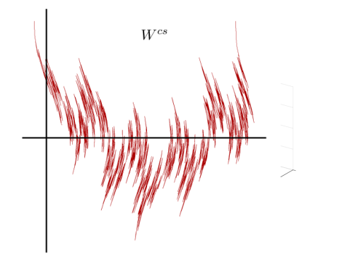
Figure 2. Top: Evolution of a curve in $W^{cu}$. Here we show the action of the map on a curve $\gamma_{0}$, $\gamma_{0}(J)\subset\{z=\mbox{constant}\}$, such that $\pi_{xy}\gamma_{0}$ is contained in a $W^{u}_{A}-$curve. The pictures on the top show the effect of $\widetilde{f}_{1}$, $\widetilde{f}_{2}$, and $\widetilde{f}_{3}$ on $\gamma_{0}$, where $\widetilde{f}_{1}$, $\widetilde{f}_{2}$, and $\widetilde{f}_{3}$ are the lifts of $f_{1}$, $f_{2}$, and $f_{3}$ respectively. Here we assume that $r(x)=x$. Bottom: action of $\widetilde{F}^{6}$ on a piece of curve $\gamma_{0}$, where $\widetilde{F}$ is the lift of the map $F$. These plots highlight the effect of the monotonicity of the coupling.

4.2.3. Persistence of splitting and foliations.

Above we showed that every skew-product map $F$ satisfying Conditions (A1)-(A3) has a continuous splitting $E^{u}\oplus E^{c}\oplus E^{s}$ defined everywhere on $\mathbb{T}^{2}\times\mathbb{T}$, and that with respect to this splitting, $DF$ satisfies a uniform domination condition. By standard invariant cones arguments, these properties are passed (with slightly relaxed bounds) to all maps $C^{1}$-near $F$. Furthermore, the foliation of $\mathbb{T}^{2}\times\mathbb{T}$ by circle fibers is smooth and by Condition (A1), also normally hyperbolic, i.e. each leaf $(x,y)\times\mathbb{T}$ is tangent to $E^{c}$ and for any $p\in(x,y)\times\mathbb{T}$

$$\|DF_{p}|_{E^{c}}\|<\|DF_{p}(\partial_{z})\|<\min_{\begin{subarray}{c}v\in E^{u},\end{subarray}{\|v\|=1}}\|DF_{p}v\|.$$

By Theorem 7.1 in [29], such a foliation, whose leaves are closed curves tangent to $E^{c}$, persists under small $C^{1}$ perturbations, although in general the perturbed foliation is only continuous. That is to say, if $F$ is a skew-product map, $\mathcal{F}$ is the foliation of $\mathbb{T}^{2}\times\mathbb{T}$ into circle fibers, and $G$ is a $C^{1}$-small perturbation of $F$, then there is a unique $G-$invariant continuous foliation $\mathcal{G}$ and a homeomorphism $H$ of $\mathbb{T}^{2}\times\mathbb{T}$ to itself that is a leaf-conjugacy, meaning $H$ carries the leaves of $\mathcal{F}$ to the leaves of ${\mathcal{G}}$, and passes to a homeomorphism $H/\sim$ from $(\mathbb{T}^{2}\times\mathbb{T})/\mathcal{F}$ to $(\mathbb{T}^{2}\times\mathbb{T})/{\mathcal{G}}$ that conjugates the two quotient dynamical systems.

4.3. Contracting centers

Returning to the skew-product map $F$, this subsection studies conditions under which $DF|_{E^{c}}$ is, on average, contracting. Such a notion requires that we specify a reference measure on unstable curves. With an eye toward SRB measures, the following is a natural choice; see e.g. [28]. For any segment of $W^{u}$-curve $W$, we let $m_{W}$ denote the arclength measure on $W$, and let $\rho_{W}:W\to\mathbb{R}$ be the function with the property that for all $p,p^{\prime}\in W$,

$$\frac{\rho_{W}(p)}{\rho_{W}(p^{\prime})}\ =\ \lim_{n\to\infty}\frac{DF^{n}_{F^{-n}p^{\prime}}|_{E^{u}}}{DF^{n}_{F^{-n}p}|_{E^{u}}}\ =\ \lim_{n\to\infty}\prod_{i=1}^{n}\frac{DF_{F^{-i}p^{\prime}}|_{E^{u}}}{DF_{F^{-i}p}|_{E^{u}}}\ ,$$ (7)

normalized so $\int_{W}\rho_{W}\ dm_{W}=1$. Because distances on $W^{u}$ contract exponentially fast in backward time, the limit above exists and convergence is exponential. Let $\mu_{W}$ be the probability measure defined by $d\mu_{W}=\rho_{W}dm_{W}$. Two useful properties of $\mu_{W}$ that can be deduced from the definition of $\rho_{W}$ are (i) $F_{*}\mu_{W}=\mu_{FW}$ where $F_{*}\mu_{W}$ is the pushforward of the measure $\mu_{W}$ by $F$, and (ii) given $\ell>0$, there is $K=K(\ell)>0$ such that for any $W$ of length $\leq\ell$ and any $p,p^{\prime}\in W$

$$\frac{\rho_{W}(p)}{\rho_{W}(p^{\prime})}\leq K\ .$$ (8)

The distortion constant $K$ depends on $\alpha^{u}_{min}$ and on the $C^{2}$ norm of $F$.

Definition 4.4.

We say $F$ satisfies a contracting center condition (with respect to the reference measures $\mu_{V}$) if there exists $c_{1}>0$ such that for any fundamental domain $V$

$$\int_{F^{-1}V}\log DF_{p}|_{E^{c}}\ d\mu_{F^{-1}V}(p)\ \leq\ -c_{1}\ .$$ (9)

The above condition, which we will henceforth abbreviate as the ``CC-condition", is reminiscent of similar conditions in the literature (see e.g. [21]). It is natural to integrate over $F^{-1}V$ (rather than $V$) because the action of $DF|_{E^{c}}$ on $F^{-1}V$ translates into the action of $g^{\prime}$ on the full circle; see (6).

Below we give a condition in terms of the various derivative bounds of $F$ (see Sect. 4.1) that implies the CC-condition. Let $I^{-}:=\{z\in\mathbb{T}:\,g^{\prime}(z)<1\}$ and $I^{+}:=\{z\in\mathbb{T}:\,g^{\prime}(z)\geq 1\}$. If $V_{A}$ is a segment of unstable leaf for the Anosov $A$, one can define $\rho_{V_{A}}$ as in (7) above by substituting $F$ with $A$. Analogous properties hold for $\rho_{V_{A}}$; we denote the distortion constant for $\rho_{V_{A}}$ by $K_{A}$.

Proposition 4.5.

Asssume (A1)-(A3). If

$$\left[\frac{CK_{A}^{2}}{c\beta}\left(1+\frac{2\lambda_{g}^{max}}{\alpha^{u}_{min}-\lambda_{g}^{max}}\right)\right]\,\int_{I^{+}}\log g^{\prime}(s)ds+\int_{I^{-}}\log g^{\prime}(s)ds<0\ ,$$ (10)

then $F$ satisfies the CC-condition.

Proof.

Let $V$ be a segment of $W^{u}$-curve of $F$ that is a fundamental domain, and let $V_{A}:=\pi_{xy}(V)$. Notice that $(\pi_{xy})_{*}\mu_{V}=\mu_{V_{A}}$, and this implies $\mu_{F^{-1}V}=(\pi_{xy}|_{F^{-1}V})^{-1}_{*}\mu_{A^{-1}V_{A}}$. Therefore,

$$\int_{F^{-1}V}\log DF_{p}|_{E^{c}}d\mu_{F^{-1}V}(p)\ =\ \int_{\mathbb{T}}\log g^{\prime}(s)\,d((\pi_{z}\circ f_{1}\circ(\pi_{xy}|_{F^{-1}V})^{-1})_{*}\mu_{A^{-1}V_{A}})(s)$$

where $f_{1}$ is as defined in Sect. 4.2.

By the change of variables formula

$$\frac{d(\pi_{z}\circ f_{1}\circ(\pi_{xy}|_{F^{-1}V})^{-1})_{*}\mu_{A^{-1}V_{A}}}{ds}(s)=\rho_{A^{-1}V_{A}}(p(s))\,D(\pi_{z}\circ f_{1}\circ\pi_{xy}^{-1}|_{A^{-1}V_{A}})^{-1}_{s},$$

where $p(s):=[\pi_{z}\circ f_{1}\circ(\pi_{xy}|_{F^{-1}V})^{-1}]^{-1}(s)$. Recall that the tangent direction to $F^{-1}V$ is $E^{u}\in\mathcal{C}^{u}_{b,a}$ which, together with assumption (A3) implies that the tangent direction to $f_{1}(F^{-1}(V))$ is in $\mathcal{C}^{u}_{b+c\beta,a+C}$, and therefore $b+c\beta\leq D(\pi_{z}\circ f_{1}\circ\pi_{xy}^{-1}|_{A^{-1}V_{A}})\leq a+C$. Recalling that $K_{A}^{-1}\leq\rho_{A^{-1}V_{A}}\leq K_{A}$ we obtain

$$[(a+C)K_{A}]^{-1}\leq\frac{d(\pi_{z}\circ f_{1}\circ(\pi_{xy}|_{F^{-1}V})^{-1})_{*}\mu_{A^{-1}V_{A}}}{ds}(s)\leq\frac{K_{A}}{c\beta}.$$

Therefore

$$\int_{F^{-1}V} \log DF_{p}|_{E^{c}}d\mu_{F^{-1}V}(p)$$

$$\leq\frac{K_{A}}{c\beta}\int_{I^{+}}\log g^{\prime}(s)ds+\left[\left(\frac{2\lambda_{g}^{max}}{\alpha^{u}_{min}-\lambda_{g}^{max}}+1\right)CK_{A}\right]^{-1}\int_{I^{-}}\log g^{\prime}(s)ds$$

and the above is strictly less than zero if condition (10) is satisfied. ∎

The following is a concrete example of a map $F$ satisfying the CC-condition. Pick any $g$ satisfying the conditions in Sect. 2.1. This condition implies that $g^{\prime}$ is not constant. By Jensen's inequality,

$$\int_{\mathbb{T}}\log g^{\prime}(s)ds<\log\int_{\mathbb{T}}g^{\prime}(s)ds=0.$$

So, there exists $\delta>0$ such that

$$(1+\delta)\int_{I^{+}}\log g^{\prime}(s)ds+\int_{I^{-}}\log g^{\prime}(s)ds<0.$$

Now pick $A$ to be any linear Anosov diffeomorphism such that $\beta=\partial_{A}^{u}\cdot\partial_{x}$ satisfies $\beta^{-1}<(1+\frac{1}{2}\delta)$. Pick $r$ also linear, i.e. $r^{\prime}=1$. Under these assumptions $K=c=C=1$ and condition (10) reads

$$\frac{1}{\beta}\left(1+\frac{2\lambda_{g}^{max}}{\alpha^{u}-\lambda_{g}^{max}}\right)\int_{I^{+}}\log g^{\prime}(s)ds+\int_{I^{-}}\log g^{\prime}(s)ds<0$$

where $\alpha^{u}$ is the uniform expansion rate of $A$. The quantity in brackets on the left can be made arbitrarily close to $1$ when $\alpha^{u}$ is sufficiently large relative to $\lambda_{g}^{max}$. It remains to ensure that $\beta$ is close to $1$. For that one can choose, e.g.,

$$A=\left(\begin{array}[]{cc}N&N-1\\ 1&1\end{array}\right)$$

for which the expanding direction is parallel to

$$\binom{{N-1+\sqrt{(N-1)(N+3)}}}{2},$$

and is therefore as aligned with the $x$-axis as we wish for $N$ sufficiently large. Notice that by picking $A$ with $\beta$ close to one and $\alpha^{u}$ large, we have also satisfied assumptions (A1)-(A3).

5. Regular Monotonic Interactions: Statistical Properties

The main result of this section, namely the existence of SRB measures for an open set of nonuniformly hyperbolic systems obtained by regular, monotonic couplings of $A$ and $g$, is stated and proved in Sect. 5.2. Uniqueness of SRB measure is proved in Sect. 5.3 under additional restrictions. Sect. 5.1 contains a brief review of SRB measures and Sect. 5.4 discusses connections to the existing literature.

5.1. SRB and physical measures

We provide here a brief review of SRB measures and physical measures; see [23] for more information.

Let $\Phi:M\circlearrowleft$ be a $C^{2}$ diffeomorphism of a compact Riemannian manifold $M$. A $\Phi$-invariant Borel probability measure $\mu$ is called an SRB measure if (i) $\Phi$ has a positive Lyapunov exponent $\mu$-a.e., and (ii) the conditional measures of $\mu$ on the unstable manifolds of $\Phi$ are absolutely continuous with respect to the Riemannian volume on these manifolds.

The following is one of the reasons why SRB measures are important. Equating observable events with sets of positive Lebesgue (or Riemannian) measure, we call an invariant Borel probability measure $\mu$ a physical measure if there is a positive Lebesgue measure set $\mathcal{B}(\mu)\subset M$ with the property that for any continuous function $h:M\to\mathbb{R}$,

$$\lim_{n\rightarrow\infty}\frac{1}{n}\sum_{i=0}^{n-1}h(\Phi^{i}x)\ =\ \int_{M}hd\mu\qquad\mbox{for every }x\in\mathcal{B}(\mu)\ .$$ (11)

This is not the Birkhoff Ergodic Theorem, as $\mu$ need not be absolutely continuous with respect to Lebesgue measure. By the absolute continuity of stable foliations, ergodic SRB measures with no zero exponents are physical measures [45], and any SRB measure with no zero Lyapunov exponents can be decomposed into at most a countable number of ergodic components each one of which is an SRB measure.

The significance of SRB measures was recognized by Sinai, Ruelle and Bowen, who constructed these measures for Axiom A attractors in the 1970s [51, 48]; see also [13]. The concept was extended to more general dynamical systems by Ledrappier, Young and others in the 1980s [40, 38, 57, 39].

Not all attractors admit SRB measures, however. Outside of the Axiom A category there are not many concrete examples; see e.g. [61, 62]. The attractors discussed in this paper are not Axiom A, but they are not far from Axiom A. They belong in a class of dynamical systems called (uniformly) partially hyperbolic systems. See Sect. 5.4 below for a more detailed discussion.

5.2. Open sets of nonuniformly hyperbolic maps with SRB measures

Let Diff${}^{2}(\mathbb{T}^{2}\times\mathbb{T})$ denote the set of $C^{2}$ diffeomorphisms of $\mathbb{T}^{2}\times\mathbb{T}$ onto itself equipped with the $C^{2}$ topology. The following is the main result of this section.

Theorem 5.1.

Let $F\in\mbox{Diff}^{2}(\mathbb{T}^{2}\times\mathbb{T})$ be the skew-product map given by Eq. (5). We assume it satisfies (A1)-(A3) in Sect. 4.1 and the CC-condition in Sect. 4.3. Then there is a neighborhood $\mathcal{N}$ of $F$ in Diff${}^{2}(\mathbb{T}^{2}\times\mathbb{T})$ such that every $G\in\mathcal{N}$ admits an SRB measure $\mu_{G}$ with one positive and two negative Lyapunov exponents.

It follows that all ergodic components of $\mu_{G}$ are physical measures.

As to whether the SRB measures in Theorem 5.1 are supported on Axiom A attractors, a straightforward extension of Proposition 4.3 to maps near $F$ that are not necessarily skew products together with the examples in Sect. 4.3 gives the following result.

Corollary 5.2.

Among the maps obtained by coupling together $A$ and $g$, there exist $C^{2}$-open sets $\mathcal{N}$ with the properties that

(i) no $G\in\mathcal{N}$ has an Axiom A attractor, and

(ii) all $G\in\mathcal{N}$ admit SRB measures.

Remark on Terminology: We have used $W^{u},W^{cu},W^{cs}$ and $W^{s}$ to denote the invariant manifolds tangent to the subbundles $E^{u},E^{c}\oplus E^{u},E^{c}\oplus E^{s}$ and $E^{s}$ respectively. This introduces a slight conflict with the usual nomenclature of stable and unstable manifolds. For example, if $DF|_{E^{c}}$ is in fact contracting, as in the case where the CC-condition is satisfied, then our $W^{cs}$-manifolds are what is usually referred to as stable manifolds, and our $W^{s}$-manifolds are what is usually called strong stable manifolds. In the interest of notational consistency among the different sections within this paper, we will adhere to the notation that $W^{*}$ denotes the invariant manifolds tangent to $E^{*}$ for $*=u,cu,s$, and $cs$; but to avoid confusion, we will refrain from using the terms ``stable manifolds" or ``unstable manifolds" in technical proofs.

Proof of Theorem 5.1.

Let $F$ be as in Theorem 5.1. Recall from Sect. 4.2.3 that any sufficiently small $C^{1}$-perturbation $G$ of $F$ inherits a dominated splitting $E^{s}\oplus E^{c}\oplus E^{u}$. We note also that the definitions of fundamental domains and the CC-condition (as defined in Sects. 4.2.2 and 4.3 for skew-product maps) carry over to $G$ provided $G$ is $C^{2}$ close to $F$. Steps 1 and 2 below prove the existence of an SRB measure for $G$ assuming it satisfies the CC-condition. Step 3 justifies the CC-condition for all $G$ sufficiently close to $F$ in the $C^{2}$-norm.

1. Construction of invariant probability measures with absolutely continuous conditional measures on $W^{u}$-leaves. We follow the standard construction of SRB measures for Axiom A attractors in e.g. [60]: Let $W$ be any finite segment of $W^{u}$-leaf for $G$, and let $m_{W}$ be the arclength measure on $W$. Letting

$$\mu_{n}\ :=\ \frac{1}{n}\sum_{i=0}^{n-1}G^{n}_{*}(m_{W})\ ,$$

we are assured that a subsequence of $\mu_{n}$ will converge weakly, and any limit point $\mu_{\infty}$ is easily shown to have absolutely continuous conditional measures on $W^{u}$-leaves. Moreover, if $\eta$ is a partition of $\mathbb{T}^{2}\times\mathbb{T}$ whose elements are unstable curves of finite length, then the condition probability densities of $\mu_{\infty}$ on any $W\in\eta$ is precisely $\rho_{W}$, the reference measures introduced in Sect. 4.3.

2. Proof of SRB property assuming the CC-condition. We now prove that any $\mu_{\infty}$ constructed in Item 1 above is an SRB measure assuming that $G$ satisfies the CC-condition. To do that, it suffices to show that $\mu_{\infty}$-a.e., the Lyapunov exponent in the $E^{c}$-direction is strictly negative.

Observe first that almost every ergodic component of $\mu_{\infty}$ has conditional densities on $W^{u}$-leaves. This is because all points on a $W^{u}$-leaf have the same asymptotic distribution in backwards time, so they cannot be generic with respect to distinct ergodic measures.

Now let $\eta$ be a measurable partition of $M=\mathbb{T}^{2}\times\mathbb{T}$ with the property that the elements $W$ of $\eta$ are fundamental domains of $W^{u}$-leaves (for instance we can pick $\pi_{z}(\partial W)=\{z_{a}\}$). Let $\mu$ be an ergodic component of $\mu_{\infty}$, and let $\{\mu_{V},V\in G^{-1}\eta\}$ be a regular family of conditional probability measures on $G^{-1}\eta$. Letting $\mu/G^{-1}\eta$ denote the quotient measure of $\mu$ on $M/G^{-1}\eta$, we have

$$\int\log DG_{p}|_{E^{c}}\ d\mu(p)=\int_{M/G^{-1}\eta}d(\mu/G^{-1}\eta)(V)\int_{V}\log DG_{p}|_{E^{c}}\ d\mu_{V}(p)\ .$$

The CC-condition says precisely that for each $V\in G^{-1}\eta$, the $d\mu_{V}$-integral is strictly negative. Thus the integral on the left is strictly negative, implying, by ergodicity of $\mu$, that the Lyapunov exponent in the $E^{c}$-direction is strictly negative $\mu$-a.e. Thus it holds $\mu_{\infty}$-a.e. since it holds for every ergodic component $\mu$ of $\mu_{\infty}$.

3. Openness of the CC-condition. We will show that if $F$ satisfies the CC-condition with constant $c_{1}$ in Eq. (9), then for small enough $\delta>0$, every $G\in\mbox{Diff}^{2}(\mathbb{T}^{2}\times\mathbb{T})$ with $d_{C^{2}}(G,F)<\delta$ will satisfy the CC-condition with constant $\frac{1}{2}c_{1}$. As we will be comparing estimates for $G$ to those of $F$, let us agree to use ordinary notation for $G$ and put a bar above quantities associated with $F$.

Let $V$ a fundamental domain for $G$. Then there is a fundamental domain $\overline{V}$ of $F$ that can be made arbitrarily close to $V$ in the sense that there is a $C^{2}$ embedding $\iota:V\rightarrow\mathbb{T}^{2}\times\mathbb{T}$ such that $\iota(V)=\overline{V}$ satisfying the following conditions as $d_{C^{2}}(G,F)\to 0$:

(a) $$d_{C^{1}}(\iota,\operatorname{Id}|_{V})\to 0,$$

(b) $$\sup_{p\in G^{-1}V}\left|DG_{p}|_{E^{c}}-DF_{\iota(p)}|_{\overline{E}^{c}}\right|\ \to\ 0\ ,$$

(c) $$\sup_{p\in G^{-1}V}\left|\rho_{G^{-1}V}(p)-\overline{\rho}_{F^{-1}\overline{V}}(\iota(p))\right|\ \to\ 0.$$

The assertions in (a) and (b) follow from Sect. 4.2.3, and the assertion in (c) follows from the fact that the distortion estimate in (7) converges exponentially fast in $n$ so it suffices to control them for a finite number of iterates. More precisely, for any $\varepsilon>0$ there is $N\in\mathbb{N}$ such that for every fundamental domain $V$ and any $p,p^{\prime}\in G^{-1}V$,

$$\frac{\rho_{{G}^{-1}V}(p)}{\rho_{{G}^{-1}V}(p^{\prime})}\leq(1+\mathcal{O}(\varepsilon))\prod_{i=1}^{N}\frac{(D{G}_{{G}^{-i}p^{\prime}})|_{E^{u}}}{(D{G}_{{G}^{-i}p})|_{E^{u}}},$$

and an analogous inequality holds for fundamental domains of $F$. Moreover, control of the differences in all three items (a), (b), and (c) above is uniform in $V$ and for all $G$ with $d_{C^{2}}(G,F)<\delta$ for small enough $\delta$. ∎

5.3. Uniqueness of SRB measures

The setting is as in Theorem 5.1. Our objective here is to investigate the uniqueness of the SRB measure for $G\in\mathcal{N}$. Assume without loss of generality that the Anosov diffeomorphism $A$ has a fixed point at $(0,0)$. Then $F$ leaves invariant the circle fiber $\{(0,0)\}\times\mathbb{T}$. By the persistence of normally hyperbolic manifolds (see (A1)), every $G\in\mathcal{N}$ leaves invariant a closed curve near $\{(0,0)\}\times\mathbb{T}$; we will call it $\mathbb{T}_{0}$.

Lemma 5.3.

For $G\in\mathcal{N}$, define

$$W^{u}(\mathbb{T}_{0}):=\cup_{p\in\mathbb{T}_{0}}W^{u}(p)\qquad\mbox{and}\qquad W^{s}(\mathbb{T}_{0}):=\cup_{p\in\mathbb{T}_{0}}W^{s}(p)\ .$$

Then (i) $W^{u}(\mathbb{T}_{0})$ and $W^{s}(\mathbb{T}_{0})$ are dense in $\mathbb{T}^{2}\times\mathbb{T}$, and

(ii) every $W^{u}$-curve meets $W^{s}(\mathbb{T}_{0})$.

Proof.

(i) We prove the claim for $W^{s}(\mathbb{T}_{0})$; the proof for $W^{u}(\mathbb{T}_{0})$ is analogous.

As $\mathbb{T}_{0}$ is invariant and normally hyperbolic, $W^{s}(\mathbb{T}_{0})$ is an immersed submanifold; see Theorem 4.1 of [29]. We know also that $W^{s}(\mathbb{T}_{0})$ is tangent to $E^{s}\oplus E^{c}$ because for every $q\in W^{s}(\mathbb{T}_{0})$, there is $p\in\mathbb{T}_{0}$ such that that $d(F^{n}p,F^{n}q)\to 0$ exponentially fast, so $q$ must have the same Lyapunov exponents as $p$.

From Sect. 4.2.3, we know that there is a $G$-invariant foliation $\mathcal{G}$ the leaves of which are closed curves tangent to $E^{c}$. This implies that $W^{s}(\mathbb{T}_{0})$ is foliated by the leaves of $\mathcal{G}$, and in fact that $W^{s}(\mathbb{T}_{0})$ is the union of $\mathcal{G}$-leaves that under iterates of $G$ tend to $\mathbb{T}_{0}$ as $n\to\infty$. Now it is also known that there is a homeomorphism $H:\mathbb{T}^{2}\times\mathbb{T}\to\mathbb{T}^{2}\times\mathbb{T}$ that is a leaf-conjugacy between $F$ and $G$, meaning it sends vertical fibers of the skew product map $F$ to the leaves of $\mathcal{G}$. Calling $\overline{\mathbb{T}}_{0}$ and $\overline{W}^{s}(\overline{\mathbb{T}}_{0})$ the corresponding objects for $F$, we have, from the characterization of $W^{s}(\mathbb{T}_{0})$ above, that $H(\overline{\mathbb{T}}_{0})=\mathbb{T}_{0}$ and $H(\overline{W}^{s}(\overline{\mathbb{T}}_{0}))=W^{s}(\mathbb{T}_{0})$. Clearly, $\overline{W}^{s}(\overline{\mathbb{T}}_{0})=W_{A}^{s}(0,0)\times\mathbb{T}$ is dense in $\mathbb{T}^{2}\times\mathbb{T}$ as the stable manifold $W_{A}^{s}(0,0)$ of $A$ is dense in $\mathbb{T}^{2}$. Therefore $W^{s}(\mathbb{T}_{0})$ is also dense since $H$ is a homeomorphism.

This completes the proof of (i).

(ii) follows immediately from the fact that $W^{s}(\mathbb{T}_{0})$ is a densely immersed submanifold tangent to $E^{c}\oplus E^{s}$. ∎

In the proofs of the results to follow, our strategy is to connect the dynamics of $G|_{\mathbb{T}_{0}}$ to those of $G$ by

– using $W^{s}(\mathbb{T}_{0})$ to draw relevant sets close to $\mathbb{T}_{0}$,

– using $G|_{\mathbb{T}_{0}}$ to transport the sets around this fixed fiber and then

– using $W^{u}(\mathbb{T}_{0})$ to deliver them to where we would like them to go.

Let $\mu$ be an ergodic SRB measure. We introduce the following definition for use below: We call a piece of $W^{u}$-leaf $W$ ``$\mu$-typical" if the following hold at $m_{W}$-a.e. $p$ (recall that $m_{W}$ is the arclength measure):

(i) $p$ is generic with respect to $\mu$, i.e., for all continuous $h:\mathbb{T}^{2}\times\mathbb{T}\to\mathbb{R}$,

$$\lim_{n\rightarrow\infty}\frac{1}{n}\sum_{i=0}^{n-1}h(G^{i}p)=\int_{\mathbb{T}^{2}\times\mathbb{T}}hd\mu;$$ (12)

(ii) $G$ has two strictly negative Lyapunov exponents at $p$ and $W^{cs}_{\rm loc}(p)$ is well defined with the property that for every $q\in W^{cs}_{\rm loc}(p)$, $d(G^{n}(p),G^{n}(q))\rightarrow 0$ as $n\rightarrow\infty$.

Let $W^{*}$ denote the set of all $p\in W$ with the properties in (i) and (ii). By the absolute continuity of $W^{cs}$-manifolds together with property (ii),

$$W^{cs}_{\rm loc}(W^{*}):=\cup_{p\in W^{*}}W^{cs}_{\rm loc}(p)$$

has positive Lebesgue measure on $\mathbb{T}^{2}\times\mathbb{T}$, and all $q\in W^{cs}_{\rm loc}(W^{*})$ are generic with respect to $\mu$.

Proposition 5.4.

If $G\in\mathcal{N}$ is such that $G|_{\mathbb{T}_{0}}$ is conjugate to an irrational rotation, then it has a unique SRB measure.

Proof.

Let $\mu_{1}$ and $\mu_{2}$ be ergodic SRB measures, and fix $W_{1}$, a $\mu_{1}$-typical $W^{u}$-curve of finite length. For $\varepsilon>0$, let $\mathcal{U}_{\varepsilon}(W_{1})$ be the tubular neighhorbood of $W_{1}$ given by $\mathcal{U}_{\varepsilon}(W_{1})=\cup_{p\in W_{1}}\mbox{exp}_{p}B^{cs}_{\varepsilon}(p)$ where $B^{cs}_{\varepsilon}(p)$ is the $\varepsilon$-ball in $E^{cs}(p)$ centered at $p$, and $\exp_{p}$ is the exponential map at $p$. We claim that there exists $\varepsilon=\varepsilon(W_{1})>0$ such that if there is a $\mu_{2}$-typical $W^{u}$-curve $W_{2}$ roughly parallel to $W_{1}$ that traverses the length of $\mathcal{U}_{\varepsilon}(W_{1})$, then $\mu_{2}=\mu_{1}$. This is true because for $\varepsilon$ small enough, there is $\Gamma\subset W^{*}_{1}$ with $m_{W_{1}}(\Gamma)>0$ such that for all $p\in\Gamma$, $W^{cs}_{2\varepsilon}(p)$ is well defined and contains a full cross-section of $\mathcal{U}_{\varepsilon}(W_{1})$. By the absolute continuity of the $W^{cs}$-foliation, $W_{2}$ will meet $\cup_{p\in\Gamma}W^{cs}_{2\varepsilon}(p)$ in a positive $m_{W_{2}}$-measure set, and all points in this set are generic with respect to $\mu_{1}$.

Since $W^{u}(\mathbb{T}_{0})$ is dense in $\mathbb{T}^{2}\times\mathbb{T}$ (Lemma 5.3 (i)), there exist $p^{\prime}\in\mathbb{T}_{0}$ and a finite-length segment $V^{\prime}$ of $W^{u}(p^{\prime})$ containing $p^{\prime}$ that crosses the length of $\mathcal{U}_{\frac{1}{4}\varepsilon}(W_{1})$. It follows that for $\varepsilon^{\prime}>0$ small enough, for all $p^{\prime\prime}\in\mathbb{T}^{2}\times\mathbb{T}$ with $|p^{\prime\prime}-p^{\prime}|<\varepsilon^{\prime}$, a subsegment $V^{\prime\prime}$ of $W^{u}(p^{\prime\prime})$ near $V^{\prime}$ will cross $\mathcal{U}_{\frac{1}{2}\varepsilon}(W_{1})$. By the topological transitivity of $G|_{\mathbb{T}_{0}}:\mathbb{T}_{0}\circlearrowleft$, there exists $\varepsilon^{\prime\prime}>0$ such that any segment of $W^{u}$-curve meeting any part of the $\varepsilon^{\prime\prime}$-neighborhood of $\mathbb{T}_{0}$ will, when iterated forward, be transported near $p^{\prime}$ and eventually cross $\mathcal{U}_{\varepsilon}(W_{1})$.

Let $W_{2}$ be any $\mu_{2}$-typical curve. By Lemma 5.3(ii), $W_{2}$ meets $W^{s}(q)$ for some $q\in\mathbb{T}_{0}$. Iterating forward, $W_{2}$ is brought as close to $\mathbb{T}_{0}$ as we wish, and by the argument above, a future iterate of $W_{2}$ – which is also $\mu_{2}$-typical – can be made to cross $\mathcal{U}_{\varepsilon}(W_{1})$ implying $\mu_{2}=\mu_{1}$. ∎

Recall that in the space of $C^{2}$ diffeomorphisms of the circle $\mathbb{T}$, an open and dense set consists of maps with a finite number of sinks and sources, and with the property that every orbit approaches a sink in forward time and a source in backward time. For $k=1,2,\cdots$, let $\mathcal{N}_{k}$ be the subset of $\mathcal{N}$ for which $F|_{\mathbb{T}_{0}}$ has the property above with exactly $k$ attractive periodic orbits. It is easy to see that $\cup_{k}\mathcal{N}_{k}$ is an open and dense subset of $\mathcal{N}$.

Theorem 5.5.

For each $k\geq 1$, there is an open and dense subset $\mathcal{N}_{k}^{\prime}\subset\mathcal{N}_{k}$ with the property that all $G\in\mathcal{N}^{\prime}_{k}$ have $\leq k$ ergodic SRB measures. In particular, uniqueness of SRB measures is enjoyed by all $G\in\mathcal{N}^{\prime}_{1}$.

Proof.

We treat first the case $k=1$, assuming that the attractive periodic cycle is a fixed point, i.e., we assume $G|_{\mathbb{T}_{\bf 0}}$ has a repelling fixed point at ${\bf 0}_{r}\in\mathbb{T}^{2}\times\mathbb{T}$, an attractive fixed point at ${\bf 0}_{a}$, and all points in $\mathbb{T}_{0}$ other than ${\bf 0}_{r}$ are attracted to ${\bf 0}_{a}$. Generalization to the periodic case is straightforward and left to the reader.

Let $G\in\mathcal{N}_{1}$. We construct an SRB measure by pushing forward Lebesgue measure on $W^{u}_{\rm loc}({\bf 0}_{a})$. Let $\mu_{1}$ be an ergodic component of the measure constructed. Let $W_{1}$ be a $\mu_{1}$-typical $W^{u}$-curve, and let $\mathcal{U}_{\varepsilon}(W_{1})$ be as in Proposition 5.3. By construction, there is a segment $V\subset W^{u}({\bf 0}_{a})$ such that $V$ crosses $\mathcal{U}_{\frac{1}{2}\varepsilon}(W_{1})$.

Let $\mu_{2}$ be another ergodic SRB measure, and let $W_{2}$ be a $\mu_{2}$-typical $W^{u}$-leaf. By Lemma 5.3(ii), $W_{2}$ meets $W^{s}(q)$ for some $q\in\mathbb{T}_{0}$. If $q\neq{\bf 0}_{r}$, then since $F^{n}q\to{\bf 0}_{a}$, $W_{2}$ will, under forward iterates, be brought as close to ${\bf 0}_{a}$ as we wish, and a future image of it will cross $\mathcal{U}_{\varepsilon}(W_{1})$ proving $\mu_{2}=\mu_{1}$.

The only problematic scenario is when $W_{2}\cap W^{s}(\mathbb{T}_{0}\setminus\{{\bf 0}_{r}\})=\emptyset$ for all $\mu_{2}$-typical curves, i.e., they meet only $W^{s}({\bf 0}_{r})$. Observe that this can happen only when $W^{u}({\bf 0}_{r})\cap W^{s}(\mathbb{T}_{0}\setminus\{{\bf 0}_{r}\})=\emptyset$, for otherwise $W_{2}$ will be brought near ${\bf 0}_{r}$ by $W^{s}({\bf 0}_{r})$; from there it will follow $W^{u}({\bf 0}_{r})$ and run into $W^{s}(\mathbb{T}_{0}\setminus\{{\bf 0}_{r}\})$ after all. It suffices therefore to show that with an arbitrarily small perturbation of $G$, one can cause $W^{u}({\bf 0}_{r})$ to intersect $W^{s}(\mathbb{T}_{0}\setminus\{{\bf 0}_{r}\})$. Such a condition is clearly open. This will be our definition of $\mathcal{N}^{\prime}_{1}$.

A specific way to make such a perturbation is as follows: Let $\Gamma^{u}$ be a segment of $W^{u}({\bf 0}_{r})$ containing ${\bf 0}_{r}$ of finite length. For $p\in\mathbb{T}^{2}\times\mathbb{T}$, let $W^{c}(p)$ denote the circle fiber tangent to $E^{c}$ through $p$, and let $W^{c}(\Gamma^{u})=\cup_{p\in\Gamma^{u}}W^{c}(p)$. Now pick $\Gamma^{s}$, a segment of $W^{s}({\bf 0}_{r})$ containing ${\bf 0}_{r}$ with the property that $W^{c}(\Gamma^{u})$ and $W^{c}(\Gamma^{s})$ meet in exactly two $W^{c}$-fibers, $\mathbb{T}_{0}$ and $W^{c}(p^{*})$ for some $p^{*}\in\Gamma^{u}$. Since by assumption, $W^{u}({\bf 0}_{r})$ does not meet $W^{s}(\mathbb{T}_{0}\setminus\{{\bf 0}_{r}\})$, we must have $p^{*}\in\Gamma^{s}$. Perturb $G$ in a small neighborhood $U$ of $G^{-1}p^{*}$ to a map $G^{\prime}$ so that $G^{\prime}(G^{-1}p^{*})\in W^{s}(\mathbb{T}_{0}\setminus\{{\bf 0}_{r}\})$. Provided that $U$ is away from ${\bf 0}_{r}$ and from $\Gamma^{s}$, we have arranged to have $W^{u}({\bf 0}_{r};G^{\prime})$ meet $W^{s}(\mathbb{T}_{0}\setminus\{{\bf 0}_{r};G^{\prime})$ where $W^{u}(\cdot;G^{\prime})$ and $W^{s}(\cdot;G^{\prime})$ refer to objects associated with the map $G^{\prime}$.

This completes the proof of the $k=1$ case.

For $k>1$, we sketch a proof again assuming (for simplicity of notation) that the attractive periodic orbits are fixed points. Let ${\bf 0}_{a,1},\cdots,{\bf 0}_{a,k}$ be the attractive fixed points, and for each ${\bf 0}_{a,i}$, construct an ergodic SRB measure $\mu_{i}$ by pushing forward Lebesgue measure on a segment of $W^{u}({\bf 0}_{a,i})$ as was done in the case $k=1$. Repeating the $k=1$ proof verbatim, we show that the $\mu_{i}$ are the only ergodic SRB measures. We do not know, however, that the $\mu_{i}$ are necessarily distinct. That is why we conclude only that the number of ergodic SRB measures is $\leq k$. ∎

5.4. Relation to the existing literature

We recapitulate the situation and discuss our results as they relate to the existing literature. For all diffeomorphisms of $\mathbb{T}^{2}\times\mathbb{T}$ that are $C^{1}$-small perturbations of the skew product maps of the form in (5), we proved the existence of a splitting $E^{u}\oplus E^{c}\oplus E^{s}$ with a uniform domination condition. General theories of hyperbolic systems with domination conditions have been studied, among others, in [15, 20, 9, 10, 1, 46] (see [29] for a more systematic treatment). Assuming additionally that the map is $C^{2}$, the existence of what is called a $u$-Gibbs measure followed [43]. Call this measure $\mu$. We further identified a checkable condition under which we proved that dynamics in the center bundle is contracting $\mu$-a.e., so that $\mu$ is in fact an SRB measure. Uniformly partially hyperbolic systems with a contracting center have been studied, among others in [11, 21, 12, 22].

What is different in this paper is that we did not start from these dynamical hypotheses. We coupled together two much studied dynamical systems in a particular way, deduced the dynamical picture above and proved the existence of SRB measures. We further demonstrated that in our setting, while the dynamics in $E^{c}$ is contracting $\mu$-a.e., the set of points at which it is asymptotically expanding is dense, showing genuinely mixed behavior in this ``neutral" direction.

These examples join the handful of concrete examples of nonuniformly hyperbolic systems known to have SRB measures, including e.g. [57, 6, 55, 41]. The examples in this paper possess invariant cones and are much closer to uniform hyperbolicity. They contribute nevertheless to expanding the relatively small group of dynamical systems known to have SRB measures.

Setups having similarities – as well as differences – to ours were considered in [7, 30, 59]. In [59], the fiber maps come from the projectivization of a 2D matrix cocycle. It is a special case of our skew-product maps; the domination condition is also different. [7] is a generalization of [59] to the skew-product setting; very high rates of expansion and contraction for $g$ are imposed. [30] builds on results from [49], and studies volume preserving perturbations of some skew-product systems (e.g. $A\times\operatorname{Id}_{\mathbb{T}}$). There volume-preservation is assumed throughout, and it is used to study finer geometric properties of the system. Our setup is more flexible, and the existence of a physical measure is not a priori guaranteed.

6. Rare but Strong Interaction

In this section, we continue to consider skew product maps of the form

$$F(x,y,z)=(A(x,y),g(z+r(x))$$ (13)

where $A:\mathbb{T}^{2}\circlearrowleft$ is an Anosov diffeomorphism, and $g$ and $r$ are as before but $r$ is a degree-one map supported on a very small interval $I_{\varepsilon}$ of length $\varepsilon>0$. We call these interactions ``rare" because a typical orbit of $A$ visits the strip $I_{\varepsilon}\times\mathbb{T}$ with frequency $\sim\varepsilon$, and when it is outside of this strip, there is no interaction between the base and the fiber map. In terms of its action on fibers, the deterministic dynamical system $F$ has the flavor of random rotations followed by long relaxation periods during which the orbit is attracted to $z_{a}\in\mathbb{T}$ (unless it is stuck at the other fixed point $z_{r}$), to be rotated again by a random amount at a random time.

6.1. Assumptions and Results

Let $\partial^{A}_{u}(\cdot)$ denote the partial derivative of a function on $\mathbb{T}^{2}$ in the direction of $E^{u}_{A}$, in the direction where $x$ is increasing. The following three conditions are assumed:

(B1) $\lambda_{g}^{max}>\max_{p}\|DA_{p}\|$

For each $\varepsilon>0$,

(B2) $r=r_{\varepsilon}:\mathbb{T}\to\mathbb{T}$ is a degree-one map with $r^{\prime}|_{I_{\varepsilon}}>0$ and $r|_{I_{\varepsilon}^{c}}=0$ where $I_{\varepsilon}\subset\mathbb{T}$ is an open interval of length $\varepsilon$.

(B3) viewing $r$ as a function on $\mathbb{T}^{2}$, we assume

$$\partial_{u}^{A}(r)>(2\varepsilon)^{-1}\quad\mbox{on }\mathbb{T}\setminus r^{-1}(-d,d)\quad\mbox{where}\quad d<\mbox{dist}(\partial I^{+},\partial(g(I^{+})))\$$

where $I^{+}$ is defined below.

Condition (B1) allows us to fix $c_{1}\in(0,1)$, a neighborhood $I^{+}$ of the repelling fixed point $z_{r}$ of $g$, and $C_{0}>1$ such that (i) $g^{\prime}\geq c_{1}^{-1}$ on $I^{+}$, and (ii) $c_{1}^{-1}>C_{0}\max_{p}\|DA_{p}\|$. This is the $I^{+}$ in (B3). Additionally we will fix $c_{0}<1$ and a neighborhood $I^{-}\subset\mathbb{T}$ of the attractive fixed point $z_{a}$ such that (i) $g^{\prime}\leq c_{0}$ on $I^{-}$ and (ii) $g(I^{+})\cap I^{-}=\emptyset$. See Figure 3 below.

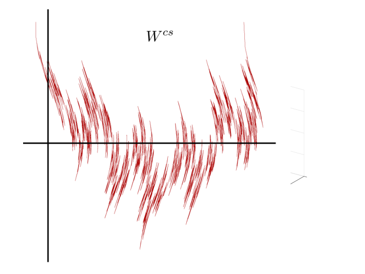
Figure 3. The pictures above illustrate assumptions (B2) and (B3). On the left is the graph of an example of $r$: $r=0$ outside of $I_{\varepsilon}$ and is very steep when $r(x)$ is in between $d$ and $1-d$. On the right is the graph of an example of $g$. The highlighted intervals are $g(I_{+})\backslash I_{+}$; each component has diameter less than $d$.

The main results of this section are as follows.

Theorem 6.1.

Given $A$ and $g$ satisfying (B1), we assume for each $\varepsilon>0$ that $r=r_{\varepsilon}$ is chosen so (B2) and (B3) are satisfied. Then for all $\varepsilon>0$ small enough, $F$ has an SRB measure $\nu_{\varepsilon}$ with two negative Lyapunov exponents. Moreover, as $\varepsilon\to 0$, $\nu_{\varepsilon}$ converges weakly to $\mu\times\delta_{z_{a}}$ where $\mu$ is the SRB measure of $A$.

The geometry of the maps satisfying (B1)-(B3) is somewhat more complicated than those studied earlier. The maps in Sects. 4 and 5 have a uniform domination condition on the entire phase space $\mathbb{T}^{2}\times\mathbb{T}$. Though there is ambiguous behavior in $E^{c}$, the directions corresponding to the strongest contraction and largest expansion are well separated. That is not so for the maps considered here: there are points whose strongest expansion occurs in the $z$-direction, and they are mixed with points with a negative Lyapunov exponent in that direction.

More precisely, consider the subset $\Gamma_{\varepsilon}$ of the horizontal section $\{z=z_{r}\}$ defined by

$$\Gamma_{\varepsilon}:=\{(x,y)\in\mathbb{T}^{2}:A^{n}(x,y)\not\in I_{\varepsilon}\mbox{ for all }n\geq 0\}\times\{z_{r}\}\ .$$

Every $p\in\Gamma_{\varepsilon}$ has two expanding directions, the stronger expansion occurring in the $z$-direction. This follows immediately from (B1) together with the fact that $F(\Gamma_{\varepsilon})\subset\Gamma_{\varepsilon}$. Geometrically, $\Gamma_{\varepsilon}$ is a Cantor set together with its stable manifolds; for $\varepsilon$ small, this set is fairly dense in $\mathbb{T}^{2}\times\{z_{r}\}$. Theorem 6.1, on the other hand, asserts that on a set of positive 3D Lebesgue measure, the Lyapunov exponent in the $z$-direction is negative. Moreover, as we will show, the unstable manifolds at $\nu_{\varepsilon}$-typical points for an SRB measure $\nu_{\varepsilon}$ crosses the horizontal section $\mathbb{T}^{2}\times\{z_{r}\}$ infinitely often.

Because of the absence of a uniform domination condition on $\mathbb{T}^{2}\times\mathbb{T}$, we have less control on the geometry of the examples here than in previous sections. In particular, we do not know if the SRB property persists under small perturbations.

6.2. Proof of Theorem 6.1

Proof.

We divide the proof into the following three steps.

1. Construction of invariant probability measures $\mu_{\varepsilon}$ with $\int\log|\partial_{z}F|d\mu_{\varepsilon}<0$. Identifying $\mathbb{T}^{2}$ with $\mathbb{T}^{2}\times\{0\}$, we let $\gamma_{0}$ be a segment of unstable manifold of $A$, and let $\gamma_{n}=F^{n}(\gamma_{0})$. Let $\mu_{0}$ be the arclength measure on $\gamma_{0}$, normalized to have total measure $1$, and let $\mu_{\varepsilon}$ be any accumulation point of $\frac{1}{n}\sum_{i=0}^{n-1}F^{i}_{*}\mu_{0}$.

We will show that for small enough $\varepsilon$, $\mu_{\varepsilon}$ has the desired property. Let $f(x,y,z)=(x,y,z+r(x))$. We need to show that a large fraction of the measure $(\pi_{z}\circ f\circ F^{n})_{*}\mu_{0}$ lies in $I^{-}$. In the argument below we will make the simplifying assumption that $A$ is linear, leaving it to the reader to insert the usual distortion estimates when it is not.

The following notation will be useful: For each $n$, let $\theta_{n}:\pi_{xy}(\gamma_{n})\to\mathbb{T}$ be such that the graph of $\theta_{n}$ is $\gamma_{n}$, and let $\psi_{n}:\pi_{xy}(\gamma_{n})\to\mathbb{T}$ be such that the graph of $\psi_{n}$ is $f(\gamma_{n})$, i.e., $\psi_{n}=\theta_{n}+r$.

At the $n$th step, let $\sigma_{n}\subset\gamma_{n}$ be a segment with $\pi_{x}\sigma_{n}=I_{\varepsilon}$. Define

$$B_{\sigma_{n},k}=\{q\in\sigma_{n}:g^{i}\pi_{z}f(q)\not\in I^{-}\mbox{ for }i=0,1,2,\cdots,k\}\ ,$$

the set of points that remain in the ``bad region" $k$ times under $g$. We claim that there exist $C_{1}>1$ independent of $\varepsilon$ such that $m_{\pi_{xy}\sigma_{n}}(\pi_{xy}B_{\sigma_{n},k})<(C_{1}\varepsilon)c_{1}^{k}$.

For $n=0$, $\sigma_{0}\subset\gamma_{0}$ is a segment with $\pi_{x}\sigma_{0}=I_{\varepsilon}$. We show that $m_{\sigma_{0}}(B_{\sigma_{0},k})<(C_{1}\varepsilon)c_{1}^{k}$ where $m_{\sigma_{0}}$ is Lebesgue measure on $\sigma_{0}$ and $c_{1}<1$ is as at the beginning of Sect. 6.1. To see this, observe that (i) $m(\pi_{z}f(B_{\sigma_{0},k}))\leq c_{1}^{k}$; (ii) on $I^{+}$ the density of $(\pi_{z}\circ f)_{*}m_{\sigma_{0}}$ with respect to Lebesgue measure $m$ on $\mathbb{T}$ is $\mathcal{O}(\varepsilon)$, because $\partial_{u}^{A}r>\frac{1}{2}\varepsilon^{-1}$ (see (B3)); and (iii) under iterates of $g$, points that leave $I^{+}$ enter $I^{-}$ a finite number of steps later.

For a general $n$, the same argument as for the case $n=0$ works, provided the condition

$$(*)\hskip 36.135pt\partial_{u}^{A}\psi_{n}>\frac{1}{2}\varepsilon^{-1}\quad\mbox{on}\quad\psi_{n}^{-1}(I^{+})\$$

is satisfied. Assuming that for now, we note that $\pi_{xy}\gamma_{n}$ has length $(\lambda^{u})^{n}$ times that of $\gamma_{0}$ where $\lambda^{u}$ is the expansion constant of $A$, so it crosses the strip $I_{\varepsilon}\times\mathbb{T}$ $\leq\mbox{const}\ (\lambda^{u})^{n}$ times. At the same time, $m_{\pi_{xy}\sigma_{n}}=(\lambda^{u})^{-n}A^{n}_{*}m_{\sigma_{0}}$, so summing $m_{\pi_{xy}\sigma_{n}}(\pi_{xy}B_{\sigma_{n},k})$ over all the components $\sigma_{n}$ of $\gamma_{n}$, one obtains for each $n$ the same estimate (up to a uniform factor) as in the $0$th step.

To estimate $g^{\prime}$ at the $n$th step, let

$${\bf B}_{n}:=\{p\in\gamma_{0}:\pi_{z}f(F^{n}(p))\not\in I^{-}\}\ .$$

Assuming (*), and adding up all the points that fell into the bad set in any one of the previous iterates and have remained there up until time $n$, we have

$$m_{\gamma_{0}}({\bf B}_{n})\leq\mbox{const}\sum_{0\leq k\leq n}(C_{1}\varepsilon)c_{1}^{n-k}\leq\mbox{const}\ (C_{1}\varepsilon)(1-c_{1})^{-1}\ .$$

In this estimate, we have overcounted in the following way: For $q\in\sigma_{i}$ for some $i$, i.e., $\pi_{x}(q)\in I_{\varepsilon}$, if it remains in the ``bad set" for $j$ iterates and $F^{j}q\in\sigma_{i+j}$, then the estimate in step $i+j$ takes over and what happened at step $i$ becomes moot but we have continued to count it in the estimate above.

This last estimate implies that for any limit point $\mu$ of $\{\frac{1}{n}\sum_{i=0}^{n-1}F^{i}_{*}\mu_{0}\}_{n=1,2,\cdots}$, we have $g^{\prime}\leq c_{0}<1$ for a fraction $1-\mathcal{O}(\varepsilon)$ of the mass. Since $g^{\prime}$ is bounded, the claim is proved for $\varepsilon$ sufficiently small.

It remains to prove (*), and we will do that inductively. Assume (*) holds at step $n-1$. We consider $\gamma_{n}$, and let $p\in\gamma_{n}$ be such that $\psi_{n}(\pi_{xy}p)\in I^{+}$ . There are several possibilities for how that could have come about:

Case 1. $\pi_{x}(p)\not\in I_{\varepsilon}$. In this case, $\theta_{n}(\pi_{xy}p)=\psi_{n}(\pi_{xy}p)\in I^{+}$, which implies $\pi_{z}f(F^{-1}p)\in I^{+}$. Condition (B1) ensures that $\partial_{u}^{A}\psi_{n}(\pi_{xy}p)=\partial_{u}^{A}\theta_{n}(\pi_{xy}p)>\partial_{u}^{A}\psi_{n-1}(\pi_{xy}F^{-1}p)$, which by hypothesis is $>\frac{1}{2}\varepsilon^{-1}$.

Case 2. $\pi_{x}(p)\in I_{\varepsilon}$ and $\theta_{n}(\pi_{xy}p)\in g(I^{+})$. This also implies $\pi_{z}fF^{-1}p\in I^{+}$. For the same reason as above, $\partial_{u}^{A}\theta_{n}(\pi_{xy}p)>\frac{1}{2}\varepsilon^{-1}$, so $\partial_{u}^{A}\psi_{n}(\pi_{xy}p)$ can only be larger.

Case 3. $\pi_{x}(p)\in I_{\varepsilon}$ and $\theta_{n}(\pi_{xy}p)\not\in g(I^{+})$. Since $\psi_{n-1}(\pi_{xy}F^{-1}p)\not\in I^{+}$, we are guaranteed only that $\partial_{u}^{A}\theta_{n}(\pi_{xy}p)\geq 0$. However, from $\theta_{n}(\pi_{xy}p)\not\in g(I^{+})$ and $\psi_{n}(\pi_{xy}p)\in I^{+}$, it follows that $r(\pi_{xy}p)\not\in(-d,d)$ (see (B3) for the definition of $d$). Hence $\partial_{u}^{A}\psi_{n}(\pi_{xy}p)\geq\partial_{u}^{A}r(\pi_{xy}p)>\frac{1}{2}\varepsilon^{-1}$ by (B3).

This completes the proof of Item 1.

2. Existence of SRB measure. Let $\mu_{\varepsilon}$ be as constructed. Since $\mu_{\varepsilon}(\mathbb{T}^{2}\times I^{-})=1-\mathcal{O}(\varepsilon)$, there is at least one ergodic component $\nu_{\varepsilon}$ of $\mu_{\varepsilon}$ with $\nu_{\varepsilon}(\mathbb{T}^{2}\times I^{-})=1-\mathcal{O}(\varepsilon)$. It follows that for $\varepsilon$ small enough, the Lyapunov exponent in the $z$-direction is strictly negative $\nu_{\varepsilon}$-a.e. We claim that $(\pi_{xy})_{*}\nu_{\varepsilon}=\mu^{A}$ where $\mu^{A}$ is the SRB measure of the Anosov map $A$. This is because $(\pi_{xy})_{*}(\frac{1}{n}\sum_{0}^{n-1}F^{i}_{*}\mu_{0})$ converges to $\mu^{A}$, so $(\pi_{xy})_{*}\mu_{\varepsilon}=\mu^{A}$, and since $\mu^{A}$ is ergodic, we have $(\pi_{xy})_{*}\nu_{\varepsilon}=(\pi_{xy})_{*}\mu_{\varepsilon}$.

We do not attempt the usual construction of SRB measures used for Axiom A attractors or in Section 5 due to technical issues with distortion estimates on unstable manifolds. Instead, we prove the SRB property of $\nu_{\varepsilon}$ by appealing to a result of [53]. Theorem C of [53] asserts that an invariant probability measure $\nu$ with no zero Lyapunov exponents is SRB if the following holds:

(*)  for any Borel set $X$ with $\nu(X)>0$, the strongly stable set of $X$,

$$\Gamma^{s}(X):=\{y\in M:\;\limsup_{n\rightarrow\infty}\log d(f^{n}x,f^{n}y)<0\mbox{ for some }x\in X\},$$

has positive Lebesgue measure.

We verify condition (*) as follows: Fix $X$ with $\nu_{\varepsilon}(X)>0$. Shrinking $X$, we may assume it consists of $\nu_{\varepsilon}$-typical points, so that at every $p\in X$, there is a 2-dimensional local stable manifold contained in $W_{A}^{s}(\pi_{xy}p)\times\mathbb{T}$ where $W^{s}_{A}(\cdot)$ is the stable manifold of $A$. These local stable disks are contained in $\Gamma^{s}(X)$.

Let $\mathcal{F}$ be the 2-dimensional foliation of $\mathbb{T}^{2}\times\mathbb{T}$ whose leaves are $W_{A}^{s}\times\mathbb{T}$. We fix a stack $\mathcal{S}$ of $\mathcal{F}$-disks with $\nu_{\varepsilon}(X\cap\mathcal{S})>0$, i.e., we fix a local unstable manifold $W$ of $A$ and a collection of disks $\{\mathcal{F}_{\alpha},\alpha\in W\}$ where $\mathcal{F}_{\alpha}$ is a disk of radius $r$ in an $\mathcal{F}$-leaf centered at $\alpha\in W$, and let $\mathcal{S}=\cup_{\alpha\in W}\mathcal{F}_{\alpha}$. As $(\pi_{xy})_{*}\nu_{\varepsilon}$ is the SRB measure of $A$, by the absolute continuity of the stable foliation of $A$, any positive $\nu_{\varepsilon}$-measure subset of $\mathcal{S}$ projects to a positive Lebesgue measure set on $W$.

Now let $m$ denote 3D Lebesgue measure on $\mathbb{T}^{2}\times\mathbb{T}$. Distintegrating $m$ into a family of regular conditional probabilities $\{m_{\alpha}\}$ on $\{\mathcal{F}_{\alpha}\}$ and a transverse measure $m_{T}$ on $W$, we have that for any Borel set $B\subset\mathbb{T}^{2}\times\mathbb{T}$,

$$m(B)=\int m_{\alpha}(B\cap\mathcal{F}_{\alpha})dm_{T}(\alpha)\ .$$ (14)

By the absolute continuity of the $\mathcal{F}$-foliation, which is an immediate consequence of the absolute continuity of the stable foliation for Anosov maps, we have that $m_{T}$ is equivalent to Lebesgue measure on $W$. As $m_{\alpha}(\Gamma^{s}(X))>0$ for a positive $m_{T}$-measure set of $\alpha$, we conclude that $m(\Gamma^{s}(X))>0$.

3. The $\varepsilon\to 0$ limit. Choosing $I^{-}$ arbitrarily small, we have $\mu_{\varepsilon}(\mathbb{T}^{2}\times I^{-})=1-\mathcal{O}(\varepsilon)$ as $\varepsilon\to 0$ though the constants depend on the size of $I^{-}$. The assertion follows. ∎

Examples of coupled systems with rare interactions in the literature include the coupled maps lattices of [35], and statistical mechanics models such as [16], [3] and [24].

7. (Straightforward) Generalizations

For conceptual clarity, we have chosen to present our results for the coupling of two specific systems: an Anosov diffeomorphism of $\mathbb{T}^{2}$ and a circle map with a sink and a source. We now discuss generalizations that are either already known, or whose proofs require only minor, nonsubstantive modifications of those in Sections 3-6.

Theorem 3.1 is valid for any diffeomorphism $F$ of a manifold of any dimension with a uniformly hyperbolic attractor and the fiber map $g$ can be any diffeomorhphism with a sink – except that the basin of the attractor need not have full Lebesgue measure. This is not new [47, 48, 58]. In the case where $A$ is an Anosov diffeomorphisms, the persistence of the attractor as an invariant manifold in the normally hyperbolic case is also well known [29].

The results of Sections 4-6 are easily extended to the following situations: The base map $A$ can be a uniformly expanding circle map (working with inverse limits); or it can be an Anosov diffeomorphism or any diffeomorphism with an Axiom A attractor. The dimension of the base manifold is irrelevant, but our proofs as given rely on the fact that $\dim(E^{u})=1$, and it is crucially important that $r$ increases monotonically along unstable curves.

An example that is especially interesting geometrically is when the base map $A:\mathbb{D}_{2}\times\mathbb{T}\circlearrowleft$ (where $\mathbb{D}_{2}$ is a 2-dimensional disk) has a solenoidal attractor, and $r$ increases monotonically as one winds around the $\mathbb{T}$-component of the base. Here we obtain an attractor in the 4-dimensional phase space $(\mathbb{T}^{2}\times\mathbb{T})\times\mathbb{T}$. Under the conditions of Sections 4 and 5, we have a ``double-frequency solenoid" whose $W^{u}$-curves wind around the two-torus in its $3$rd and $4$th dimensions in a fairly regular manner. Under the assumptions of Section 6, $W^{u}$-curves wind around the 3rd dimension in a regular fashion making abrupt excursions around the 4th. In both cases, the attractor so obtained is not uniformly hyperbolic as it has mixed behavior in the 4th dimension.

E-mail address: matteo.tanzi@nyu.edu

E-mail address: lsy@cims.nyu.edu

References

- [1] F. Abdenur, C. Bonatti, and S. Crovisier. Global dominated splittings and the Newhouse phenomenon. Proceedings of the American Mathematical Society, 134(8):2229–2237, 2006.
- [2] V. Baladi, M. Degli Esposti, S. Isola, E. Järvenpää, and A. Kupiainen. The spectrum of weakly coupled map lattices. Journal de mathématiques pures et appliquées, 77(6):539–584, 1998.
- [3] P. Bálint, T. Gilbert, P. Nándori, D. Szász, and I. P. Tóth. On the limiting Markov process of energy exchanges in a rarely interacting ball-piston gas. Journal of statistical physics, 166(3-4):903–925, 2017.
- [4] J.-B. Bardet, G. Keller, and R. Zweimüller. Stochastically stable globally coupled maps with bistable thermodynamic limit. Communications in Mathematical Physics, 292(1):237–270, 2009.
- [5] M. Benedicks and L. Carleson. The dynamics of the Hénon map. Annals of Mathematics, 133(1):73–169, 1991.
- [6] M. Benedicks and L.-S. Young. Sinai-Bowen-Ruelle measures for certain Hénon maps. In The Theory of Chaotic Attractors, pages 364–399. Springer, 1993.
- [7] K. Bjerklöv. A note on circle maps driven by strongly expanding endomorphisms on T. Dynam. Sys., 33:361–368, 2018.
- [8] S. Boccaletti, V. Latora, Y. Moreno, M. Chavez, and D.-U. Hwang. Complex networks: Structure and dynamics. Physics reports, 424(4-5):175–308, 2006.
- [9] J. Bochi and M. Viana. Lyapunov Exponents: how Frenquently are Dynamical Systems Hyperbolic? Inst. de Matemática Pura e Aplicada, 2003.
- [10] C. Bonatti, L. J. Díaz, and E. R. Pujals. A C1-generic dichotomy for diffeomorphisms: weak forms of hyperbolicity or infinitely many sinks or sources. Annals of Mathematics, pages 355–418, 2003.
- [11] C. Bonatti, M. Viana, et al. SRB measures for partially hyperbolic systems whose central direction is mostly contracting. Israel Journal of Mathematics, 115(1):157–193, 2000.
- [12] C. Bonatti and A. Wilkinson. Transitive partially hyperbolic diffeomorphisms on 3-manifolds. Topology, 44(3):475–508, 2005.
- [13] R. Bowen. Equilibrium states and the ergodic theory of anosov diffeomorphisms. Springer Lecture Notes in Math, 470:78–104, 1975.
- [14] J. Bricmont and A. Kupiainen. High temperature expansions and dynamical systems. Communications in Mathematical Physics, 178(3):703–732, 1996.
- [15] M. I. Brin and Y. B. Pesin. Partially hyperbolic dynamical systems. Uspekhi Matematicheskikh Nauk, 28(3):169–170, 1973.
- [16] L. Bunimovich, C. Liverani, A. Pellegrinotti, and Y. Suhov. Ergodic systems of balls in a billiard table. Communications in Mathematical Physics, 146(2):357–396, 1992.
- [17] L. Bunimovich and Y. G. Sinai. Spacetime chaos in coupled map lattices. Nonlinearity, 1(4):491, 1988.
- [18] J.-R. Chazottes and B. Fernandez. Dynamics of coupled map lattices and of related spatially extended systems, volume 671. Springer Science & Business Media, 2005.
- [19] H. De Jong. Modeling and simulation of genetic regulatory systems: a literature review. Journal of computational biology, 9(1):67–103, 2002.
- [20] L. J. Díaz, E. R. Pujals, R. Ures, et al. Partial hyperbolicity and robust transitivity. Acta Mathematica, 183(1):1–43, 1999.
- [21] D. Dolgopyat. On dynamics of mostly contracting diffeomorphisms. Communications in Mathematical Physics, 213(1):181–201, 2000.
- [22] D. Dolgopyat, M. Viana, and J. Yang. Geometric and measure-theoretical structures of maps with mostly contracting center. Communications in Mathematical Physics, 341(3):991–1014, 2016.
- [23] J.-P. Eckmann and D. Ruelle. Ergodic theory of chaos and strange attractors. In The theory of chaotic attractors, pages 273–312. Springer, 1985.
- [24] J.-P. Eckmann and L.-S. Young. Nonequilibrium energy profiles for a class of 1-d models. Communications in mathematical physics, 262(1):237–267, 2006.
- [25] B. Fernandez. Computer-assisted proof of loss of ergodicity by symmetry breaking in expanding coupled maps. In Annales Henri Poincaré, volume 21, pages 649–674. Springer, 2020.
- [26] T. Fischer and H. H. Rugh. Transfer operators for coupled analytic maps. Ergodic Theory and Dynamical Systems, 20(1):109–143, 2000.
- [27] D. Hadjiloucas, M. J. Nicol, and C. P. Walkden. Regularity of invariant graphs over hyperbolic systems. Ergodic Theory and Dynamical Systems, 22(2):469–482, 2002.
- [28] B. Hasselblatt and A. Katok. Handbook of dynamical systems. Elsevier, 2002.
- [29] M. W. Hirsch, C. C. Pugh, and M. Shub. Invariant manifolds (Lecture Notes in Mathematics, 583). Springer, Berlin-New York, 1977.
- [30] A. J. Homburg. Circle diffeomorphisms forced by expanding circle maps. Ergodic theory and dynamical systems, 32(6):2011–2024, 2012.
- [31] K. Kaneko. Theory and applications of coupled map lattices. Nonlinear science: theory and applications, 1993.
- [32] J. L. Kaplan, J. Mallet-Paret, and J. A. Yorke. The Lyapunov dimension of a nowhere differentiable attracting torus. Ergodic Theory and Dynamical Systems, 4(2):261–281, 1984.
- [33] G. Keller and M. Künzle. Transfer operators for coupled map lattices. Ergodic Theory and Dynamical Systems, 12(2):297–318, 1992.
- [34] G. Keller and C. Liverani. Uniqueness of the SRB measure for piecewise expanding weakly coupled map lattices in any dimension. Communications in Mathematical Physics, 262(1):33–50, 2006.
- [35] G. Keller and C. Liverani. Map lattices coupled by collisions. Communications in Mathematical Physics, 291(2):591–597, 2009.
- [36] J. Koiller and L.-S. Young. Coupled map networks. Nonlinearity, 23(5):1121, 2010.
- [37] Y. Kuramoto. Self-entrainment of a population of coupled non-linear oscillators. In International symposium on mathematical problems in theoretical physics, pages 420–422. Springer, 1975.
- [38] F. Ledrappier. Propriétés ergodiques des mesures de Sinaĭ. Publications Mathématiques de l'IHÉS, 59:163–188, 1984.
- [39] F. Ledrappier, J.-M. Strelcyn, et al. A proof of the estimation from below in Pesin entropy formula. CSP, Dép. de mathématiques, 1981.
- [40] F. Ledrappier and L.-S. Young. The metric entropy of diffeomorphisms: Part I: Characterization of measures satisfying Pesin's entropy formula. Annals of Mathematics, pages 509–539, 1985.
- [41] K. Lu, Q. Wang, and L.-S. Young. Strange attractors for periodically forced parabolic equations, volume 224. American Mathematical Soc., 2013.
- [42] T. Pereira, S. van Strien, and M. Tanzi. Heterogeneously coupled maps: hub dynamics and emergence across connectivity layers. Journal of the European Mathematical Society, doi: 10.4171/JEMS/963, Electronically published on April 2, 2020.
- [43] Y. B. Pesin and Y. G. Sinai. Gibbs measures for partially hyperbolic attractors. Ergodic Theory and Dynamical Systems, 2(3-4):417–438, 1982.
- [44] A. Pikovsky, J. Kurths, M. Rosenblum, and J. Kurths. Synchronization: a universal concept in nonlinear sciences, volume 12. Cambridge university press, 2003.
- [45] C. Pugh and M. Shub. Ergodic attractors. Transactions of the American Mathematical Society, 312(1):1–54, 1989.
- [46] E. R. Pujals and M. Sambarino. On the dynamics of dominated splitting. Annals of Mathematics, pages 675–739, 2009.
- [47] C. Robinson. Structural stability of diffeomorphisms. Journal of Differential Equations, 22(1):28–73, 1976.
- [48] D. Ruelle. A measure associated with axiom-A attractors. American Journal of Mathematics, pages 619–654, 1976.
- [49] D. Ruelle and A. Wilkinson. Absolutely singular dynamical foliations. Communications in Mathematical Physics, 219(3):481–487, 2001.
- [50] F. Sélley and P. Bálint. Mean-field coupling of identical expanding circle maps. Journal of Statistical Physics, 164(4):858–889, 2016.
- [51] Y. G. Sinai. Gibbs measures in ergodic theory. Russian Mathematical Surveys, 27(4):21, 1972.
- [52] S. H. Strogatz and I. Stewart. Coupled oscillators and biological synchronization. Scientific American, 269(6):102–109, 1993.
- [53] M. Tsujii. Regular points for ergodic Sinaĭ measures. Transactions of the American Mathematical Society, 328(2):747–766, 1991.
- [54] J. D. Wang and P. A. Levin. Metabolism, cell growth and the bacterial cell cycle. Nature Reviews Microbiology, 7(11):822–827, 2009.
- [55] Q. Wang and L.-S. Young. From invariant curves to strange attractors. Communications in Mathematical Physics, 225(2):275–304, 2002.
- [56] Q. Wang and L.-S. Young. Toward a theory of rank one attractors. Annals of Mathematics, pages 349–480, 2008.
- [57] L.-S. Young. Bowen-Ruelle measures for certain piecewise hyperbolic maps. In The Theory of Chaotic Attractors, pages 265–272. Springer, 1985.
- [58] L.-S. Young. Large deviations in dynamical systems. Transactions of the American Mathematical Society, 318(2):525–543, 1990.
- [59] L.-S. Young. Some open sets of nonuniformly hyperbolic cocycles. Ergodic Theory and Dynamical Systems, 13(2):409–415, 1993.
- [60] L.-S. Young. Ergodic theory of differentiable dynamical systems, volume Real and Complex Dynamics of NATO ASI series, pages 293–336. Kluwer Academic Publishers, ed. branner and hjorth edition, 1995.
- [61] L.-S. Young. Statistical properties of dynamical systems with some hyperbolicity. Annals of Mathematics, 147(3):585–650, 1998.
- [62] L.-S. Young. What are SRB measures, and which dynamical systems have them? Journal of Statistical Physics, 108(5):733–754, 2002.
- [63] L.-S. Young. Towards a mathematical model of the brain. Journal of Statistical Physics, pages 1–18, 2020.