Electrical band flattening, valley flux, and superconductivity in twisted trilayer graphene

Abstract

Twisted graphene multilayers have demonstrated to yield a versatile playground to engineer con- trollable electronic states. Here, by combining first-principles calculations and low-energy models, we demonstrate that twisted graphene trilayers provide a tunable system where van Hove singularities can be controlled electrically. In particular, it is shown that besides the band flattening, bulk valley currents appear, which can be quenched by local chemical dopants. We finally show that in the presence of electronic interactions, a non-uniform superfluid density emerges, whose non-uniformity gives rise to spectroscopic signatures in dispersive higher energy bands. Our results put forward twisted trilayers as a tunable van der Waals heterostructure displaying electrically controllable flat bands and bulk valley currents.

I Introduction

The interplay between topology and correlations represents a highly fruitful area in condensed matter physics. However, exploring unconventional states of matter requires identifying systems where electronic correlations, topology and electronic dispersions can be realistically controlled. In this line, twisted van der Waals materialsCao et al. (2018); Yankowitz et al. (2019); Liu et al. (2014); Lu et al. (2019); Rickhaus et al. (2018); San-Jose and Prada (2013); Liao et al. (2020); Shimazaki et al. (2020) provide a powerful solid state platform to realize exotic quantum phenomena. The tunability of twisted van der Waals materials stems from the emergence of a band structure that can be controlled by the twist between different two-dimensional materials.Lopes dos Santos et al. (2007); Suárez Morell et al. (2010) In particular, the different quantum states in twisted graphene systems stem from the possibility of controlling the ratio between kinetic and interaction terms. In twisted graphene bilayers, such tunability allowed to realize superconducting,Cao et al. (2018); Yankowitz et al. (2019); Lu et al. (2019) correlated insulators, topological networks,Rickhaus et al. (2018); San-Jose and Prada (2013) Chern insulatorsSerlin et al. (2019) and quasicrystals.Ahn et al. (2018); Moon et al. (2019); Yu et al. (2019); Pezzini et al. (2020) As a result, current experimental efforts are focusing on exploring new twisted van der Waals materials, with the aim of finding platforms that allow for an even higher degree of control.Chen et al. (2020); Polshyn et al. (2020)

From the quantum engineering point of view, applying a perpendicular bias between layersCastro et al. (2007) provides a versatile way of tuning correlated states in twisted graphene multilayers. This has been demonstrated in paradigmatic examples of correlated states in twisted tetralayers (double bilayer)Liu et al. (2019); Shen et al. (2020) and twisted trilayers (monolayer/bilayer).Chen et al. (2020); Polshyn et al. (2020) Moreover, interlayer bias is known to generate internal valley currents in twisted graphene bilayers,Rickhaus et al. (2018); San-Jose and Prada (2013); Ramires and Lado (2018); Wolf et al. (2019a) creating topological networks at low anglesRickhaus et al. (2018); San-Jose and Prada (2013); Ramires and Lado (2018) and generating valley fluxes in flat bands regimes.Wolf et al. (2019a) This interplay of correlations and topology in twisted graphene multilayers makes these materials a powerful platform to explore exotic states of matterAbouelkomsan et al. (2020); Liu et al. (2020); Repellin and Senthil (2019); Ledwith et al. (2019) in a realistically feasible manner.

From the theoretical point of view, electronic structure calculation of twisted graphene bilayer conducted with real-space tight-binding modelsSuárez Morell et al. (2010) or continuum Dirac descriptionsLopes dos Santos et al. (2007) capture the fundamental features of the electronic dispersion. Nevertheless, internal coordinates optimization can quantitatively modify the electronic dispersion.Carr et al. (2018); Lin et al. (2018); Nam and Koshino (2017); Leconte et al. (2019); Brihuega and Yndurain (2017); Koshino and Son (2019); Angeli et al. (2019); Rickhaus et al. (2019) Well known examples of this are the growth of AB/BA regions in twisted bilayers.Nam and Koshino (2017); Ochoa (2019) It is important to note that studying twisted graphene multilayers from first-principles represents a remarkable challenge, due to the large amount of atoms present in a unit cell.

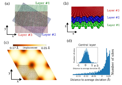
Figure 1: (a,b) Sketch of the structure a twisted graphene trilayer, in which the top and bottom layers are aligned, and twisted with respect the middle one. Panel (c) shows the color map of a DFT-based relaxed 2$\times$2 supercell of twisted trilayer. Colored pattern corresponds to the difference $\Delta=z-z_{av}$ between the z coordinate of an atom in surface layer and the average coordinate $z_{av}$ of all atoms in the same layer. AA stacking regions are colored with darker tones whereas AB/BA stacking regions are colored with lighter tones. Superimposed is the unit cell of the trilayer. Panel (d) shows the histogram shows the number of occurrences of each distance to the average deviation value. Tiny deviations from flatness occur in the central layer. Calculations performed with DFT.

Here, by combining first-principles calculations and low-energy models, we show that twisted graphene trilayersSuárez Morell et al. (2013) host flat bands whose bandwidth can be controlled electrically. We address the impact of an interlayer bias both from first-principles and effective models, showing that van Hove singularities can be merged electrically. We show that associated with the interlayer bias, bulk valley currents emerge, that are impacted by the existence of chemical impurities in the system. We finally address the superconducting states in these doped trilayers, showing that the non-uniform superfluid density has an impact in high-energy bands. Our manuscript is organized as follows, in Sec. II we show the electronic structure of twisted graphene trilayer both from first-principles and low-energy models, in Sec. III we explore in detail the impact of an electric field, in Sec. IV we explore the effect of chemical impurities, and in Sec. V we address the impact of an emergent non-uniform superfluid density. Finally, in Sec. VI we summarize our conclusions.

II Electronic structure of twisted trilayer graphene

The electronic structure of twisted graphene trilayersSuárez Morell et al. (2013); Li et al. (2019); Khalaf et al. (2019); Carr et al. (2019); Mora et al. (2019); Park et al. (2020) shows different features in comparison with twisted graphene bilayers.Suárez Morell et al. (2010); Bistritzer and MacDonald (2011) The electronic structure of small ”magic” angle tBLG features four flat bands lying around the Fermi level, with band splitting at the $\Gamma$ point of the Brillouin zone of the emergent moiré superlattice.Suárez Morell et al. (2010); Bistritzer and MacDonald (2011) Density functional theory (DFT) calculations have shown consistent results with those effective models in twisted graphene multilayers, yet quantitative modifications are observed when including relaxation of the atomic coordinatesNam and Koshino (2017); Angeli et al. (2018); Leconte et al. (2019); Lucignano et al. (2019); Cantele et al. (2020) and crystal-field effectsRickhaus et al. (2019); Haddadi et al. (2020). Therefore, to benchmark the electronic properties of twisted graphene multilayers, it is essential to start from a correct description that takes into account the geometric corrugation and ab-initio electrostatics of the moiré system.

We consider a twisted trilayer structure in which the upper and lower layers are aligned, and the middle one is twisted with an angle $\theta$ with respect to those (Fig. 1ab). In particular, in the following we will consider a twisted trilayer whose middle layer has a twisting angle of 1.9^∘ with respect to the external layers. A twisted multilayer like this can be created with standard tear, rotate and stack techniques.Kim et al. (2016) The system of 5514 atoms is fully relaxed allowing for lateral and vertical displacement of the C atoms in the structure. Figure 1c shows the color map of one of the two equivalent external layer relaxation. The color scheme represents the vertical variation of each C atom at the surface with respect to the average deviation within each layer. The darker areas indicate a displacement of atoms out of the surface which occurs predominantly in the AA stacking region. The histogram of Fig. 1d shows that the number of atoms in the upper layer whose vertical coordinate is above the average is twice as large as the atoms displaced in the opposite direction below the average.

The first-principles electronic band diagram of the fully relaxed structure of $\theta=1.9^{\circ}$ TTG is shown in Fig. 2. In contrast with twisted bilayer graphene, two highly dispersive bands coexist with four low-dispersive bands grouped at the Fermi energy. The Dirac-like crossing above the charge neutrality point leads to a small charge transfer between the flat and dispersive bands even at half filling. Additional flattening of the localized states can be induced by application of an external electric field perpendicular to the TTG surface. A field of 0.03 eV/Å reduces the dispersion of all electronic states in the vicinity of the Fermi energy without inducing any inter-band charge transfer. Increasing the strength up to 0.25 eV/Å a disruption of the linear bands is observed and a hybridization of the flat bands with neighboring state increase their dispersion. It is observed that the application of an interlayer bias generates Dirac crossings above and below charge neutrality, besides a variety of anticrossings (Fig. 2).

The first-principles calculations above show that the electronic structure of twisted trilayer graphene show strong differences with the one of twisted graphene bilayers. In particular, a highly dispersive set of bands coexists with the nearly flat bands at charge neutrality. In order to explore more in detail the physics and twisted trilayers, in the following we will exploit a low-energy model. We find that the tight binding model qualitatively reproduces the important features of the band structure without including relaxations and additional charge transfer effects. Therefore, for the sake of simplicity we now take an unrelaxed structure for our tight binding calculations. We take a single orbital per carbon atom, yielding a tight-binding Hamiltonian of the form

$$\mathcal{H}_{0}=-t\sum_{\langle i,j\rangle,s}c_{i,s}^{\dagger}c_{j,s}-\sum_{i,j,s}\bar{t}_{\perp}({\mathbb{r}}_{i},{\mathbb{r}}_{j})c_{i,s}^{\dagger}c_{j,s},$$ (1)

with $\bar{t}_{\perp}(\mathbb{r}_{i},\mathbb{r}_{j})=t_{\perp}\frac{(z_{i}-z_{j})^{2}}{|\mathbb{r}_{i}-\mathbb{r}_{j}|^{2}}e^{-\beta(|\mathbb{r}_{i}-\mathbb{r}_{j}|-d)}$, where $d$ is the interlayer distance and $\beta$ controls the decay of the interlayer hopping. As a reference, for twisted graphene multialyers $t\approx 3$ eV and $t_{\perp}\approx 0.15t$. Similar real-space models were used to study a variety of twisted graphene multilayers,Suárez Morell et al. (2010, 2013, 2010); Culchac et al. (2019); Morell et al. (2015) providing a simple formalism to study the effect of dopands and impurities.Ramires and Lado (2019); Lopez-Bezanilla and Lado (2019) However, in contrast to continuum models,Lopes dos Santos et al. (2012, 2007); Bistritzer and MacDonald (2011) measuring of valley related quantities with a real-space based formalism is non-trivial.

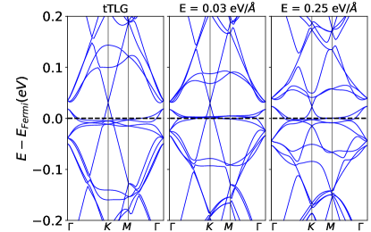
Figure 2: Electronic band diagrams of twisted trilayer graphene. Localized states at the Fermi energy coexist with highly dispersive states bands forming a Dirac cone in the conduction band. Applying a small electric field perpendicular to the TTG a reduction of all bands dispersion is induced. A stronger electric field removes the Dirac cones and induces hybridization between electronic states. Calculations performed with DFT

Twisted graphene multilayers own an approximate symmetry associated to the valley quantum number.Lopes dos Santos et al. (2007) Valley physics in both DFT calculations and tight-binding are emergent symmetries, in the sense that valley are not easily defined in terms of real-space chemical orbitals. This limitation can be overcome by defining the so-called valley operatorColomés and Franz (2018); Ramires and Lado (2018, 2019) in the tight-binding description. With the valley operator the expectation value of the valley can be computed in a real space representation.Wolf et al. (2019b); Manesco et al. (2020) The details of the valley operatorColomés and Franz (2018); Ramires and Lado (2018, 2019) are given in Sec. B, in the following we will take as starting point the valley operator $\mathcal{V}_{z}$ With the previous operator, we can compute the valley flavor of each eigenstate of the twisted trilayer supercell within the real-space formalism as $\langle\mathcal{V}_{z}\rangle=\langle\Psi|\mathcal{V}_{z}|\Psi\rangle|$. It is worth noting that this operator can be easily defined in the tight-binding basis but not in the DFT basis. We finally note that the valley operator $\mathcal{V}_{z}$ in the twisted moire system will show the valley flavor in the original Brillouin zone of graphene, not the mini-Brillouin zone of the twisted system.

With the previous formalism, we now compute the electronic structure of the low-energy model at the same angle $\theta=1.9^{\circ}$ as in the first-principles calculations (Fig. 3). We note that, besides some additional splittings observed in the first-principles calculations (Fig. 2), the band-structure obtained with the low-energy model (Fig. 3ab) gives comparable results. As shown in Fig. 3a, in the absence of an interlayer bias the system shows nearly flat bands coexisting with highly dispersive states. Whereas the nearly flat bands are degenerate in valleys in the path shown, the dispersive states belong to different valleys in different parts of the Brillouin zone. It is also observed that the dispersive Dirac cones are slightly displaced from charge neutrality, as observed in the first principles results.

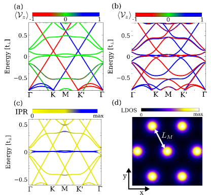
Figure 3: (a) Band structure of a twisted trilayer at angle of 1.9^∘, without (a) and with (b) interlayer bias, showing analogous dispersion to those found by first principles in Fig. 2. Panel (c) shows the band structure at a lower angle of $\theta=1.6^{\circ}$, showing a flattening of the bands. Panel (d) shows the local density of states at the Fermi energy, showing a triangular supercell pattern. Note that part of the k-path is different in comparison with Fig. 2. Calculations performed with tight-binding.

We now move on to considered the effect of the itnerlayer bias. An interlayer bias can be easily included in the low-energy tight-binding model by means of

$$\mathcal{H}_{V}=V/(2d)\sum_{i,s}z_{i}c^{\dagger}_{i,s}c_{i,s}$$ (2)

where $z_{i}$ is the $z$-position of site $i$, $d$ is the interlayer distance and $V$ is the strength of the interlayer bias. The full Hamiltonian in the presence of interlayer bias is thus $\mathcal{H}=\mathcal{H}_{0}+\mathcal{H}_{V}$. When an interlayer bias is turned on (Fig. 3b), the valley degeneracy in the $G-K$ path is lifted, and the dispersive bands show two crossings above and below the nearly flat bands, analogously to the first-principles results. It is also observed that the nearly flat bands are slightly modified by the interlayer bias. As we will show below, such effect becomes stronger for even smaller angles.

A last interesting point is related with the the localization of the different states in the supercell. This can be characterized by means of the inverse participation ratio (IPR), defined as $IPR=\sum_{i}|\Psi_{k}(i)|^{4}$. Large values of the IPR correspond to states localized in the moiré supercell, whereas low values correspond to delocalized in the moiré supercell. Focusing now in a structure with $\theta=1.6^{\circ}$ twisting angle, it is clearly observed that the nearly flat bands show a substantially higher degree of localization than the dispersive bands (Fig. 3c). In particular, the flat band states are associated to an emergent triangular lattice in the supercell, as shown in the local density of states (LDOS) of Fig. 3d. In the following we will see how these flat band states can be electrically controlled, and how the bias creates bulk valley currents associated with the valley splittings.

III Band flattening and valley currents by an interlayer bias

We now move on to systematically analyze the effect of an interlayer bias in the twisted graphene trilayer, and in particular its effect on the low energy density of states. Electric biases in twisted graphene multilayers are known to give rise to valley Hall currents,McCann (2006); Martin et al. (2008); Zhang et al. (2013); Mañes et al. (2007); San-Jose and Prada (2013); Ramires and Lado (2018); Rickhaus et al. (2018) and represent an effective knob to control the low-energy electronic structure.Castro et al. (2007) In the following we focus on the structure at $\theta=1.6^{\circ}$. As shown in Fig. 4a, the application of an interlayer bias merges the original two van Hove singularities of zero bias in a single one, dramatically enhancing the low-energy density of states. Interestingly, this merging of van Hove singularities is similar to the evolution with the twist angle in twisted bilayers,Suárez Morell et al. (2010); Bistritzer and MacDonald (2011); San-Jose et al. (2012) with the key difference that in the present case the merging is electrical, turning the process highly controllable in-situ.

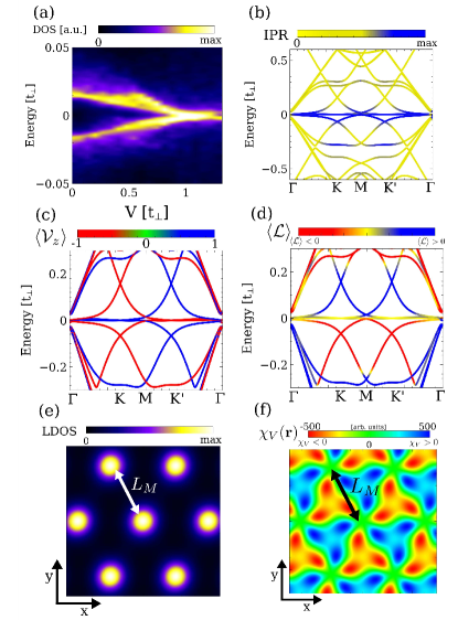
Figure 4: (a) Evolution of the density of states as a function of the interlayer bias for $\theta=1.6^{\circ}$. Panel (b) shows the band structure at a finite electric field depicting the localization of each state of each state. Panel (c) shows the valley polarization of the low-energy states, whereas panel (d) their layer polarization. Panel (e) shows the spatial localization of the nearly flat bands. Panel (f) shows the local valley flux at one electron per unit cell. The spatial maps in (e,f) are summed over the three layers. Calculations performed with tight-binding.

We now focus on the flattest regime with finite bias, when the two van Hove singularities get merged. Fig. 4bcd shows the band structure of that regime . It is observed that almost perfectly flat bands are present at the Fermi energy (Fig. 4bcd), accounting for the van Hove singularity at charge neutrality (Fig. 4a). It is also observed that the states remain highly localized in the unit cell as highlighted by the IPR, whereas at higher energies the dispersive bands are delocalized in the moiré unit cell (Fig. 4b). It is also observed that the bands show perfect valley polarization (Fig. 4c), so that the interlayer bias does create any intervalley scattering in agreement with continuum models. Given that the interlayer bias breaks the symmetry between the top and bottom layers, it is interesting to look at the layer polarization of the states $\langle\mathcal{L}\rangle$, defined by the layer polarization operator $\mathcal{L}=\sum_{i,s}z_{i}c^{\dagger}_{i,s}c_{i,s}$, with $z_{i}$ the $z$-component of the site $i$. As shown in Fig. 4d, the Dirac cones at the $K,K^{\prime}$ points above and below the flat bands have a slightly opposite layer polarization. However, such layer polarization is reversed at the $\Gamma$ point (Fig. 4d), highlighting that the states remain highly entangled between all the layers.

We now explore how the band flattening is accompanied with the emergence of bulk valley currents. The emergence of valley currents associated with interlayer biases is a well known effect in aligned graphene bilayersMcCann (2006); Martin et al. (2008); Zhang et al. (2013); Mañes et al. (2007) and tiny-angle twisted bilayers.San-Jose and Prada (2013); Ramires and Lado (2018); Rickhaus et al. (2018) Such valley currents arise due to the emergence of valley a non-zero local valley Chern numbers,Ren et al. (2016) whose quantization is associated to the emergent valley conservation.Castro Neto et al. (2009) In twisted systems, the local Chern number is expected to change from region to region,San-Jose and Prada (2013) due to the locally modulated Hamiltonian. To address this local topological property, in the following we compute the local valley flux by means of the Berry flux density $\chi_{V}$. The real-space valley flux $\chi_{V}$ defines the valley Chern number as $C_{V}=C_{K}-C_{K^{\prime}}=\int\chi_{V}(\mathbf{r},\omega)d^{2}\mathbf{r}d\omega$. The real-space valley flux $\chi_{V}$ can be computed asChen and Lee (2011); Wolf et al. (2019b); Manesco et al. (2020)

$$\chi_{V}(\mathbf{r},\omega)=\int\frac{d^{2}\mathbf{k}}{(2\pi)^{2}}\frac{\epsilon_{\alpha\beta}}{2}\langle\mathbf{r}|G_{V}(\partial_{k_{\alpha}}G_{V}^{-1})(\partial_{k_{\beta}}G_{V})|\mathbf{r}\rangle$$ (3)

where $\epsilon_{\alpha\beta}$ denotes the Levi-Civita tensor, $G_{V}$ the valley Green’s function $G_{V}=[\omega-\mathcal{H}_{\mathbf{k}}+i0^{+}]^{-1}\mathcal{V}_{z}$, $\mathcal{H}_{k}$ the Bloch Hamiltonian, and $\mathcal{V}_{z}$ the valley polarization operator of Eq. 5.

Fig. 4f shows the spatial profile of the valley flux density at the Fermi energy $\chi_{V}(\mathbf{r})\equiv\chi_{V}(\mathbf{r},\omega=\epsilon_{F})$, for a chemical potential with one hole per unit cell. It can be observed clearly that sizable valley currents appear in regions in the complementary regions to the low-energy states, similarly to other moiré systems.Wolf et al. (2019b); Manesco et al. (2020). Since the emergence of such currents relies on valley conservation, terms in the system creating intervalley mixing are expected to substantially impact them,San-Jose and Prada (2013); Tkachov and Hentschel (2012); Yan et al. (2016); Rodrigues (2016) as we address in the next section.

IV Impact of chemical doping

In this section we address the modification of the electronic structure under both electrical and chemical doping. First, we start with the study of the electric doping from first-principles, and afterwards we move on to consider its effect in the low-energy effective model.

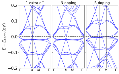
Figure 5: Electronic band diagrams of three doped TTG configurations. Left panel shows electrostatic doping with one extra electron. Central panel shows that doping with a N atom causes a similar effect but removes the Dirac point and converts TTG in a tiny-gap semiconductor. Right panel shows that doping with a B atom empties some bands at the Fermi level including the highly dispersive bands. Calculations performed with DFT.

We first address the impact of doping from first-principles. First-principles DFT calculations are employed to study the modification of the band diagram of TTG upon doping with both an extra charge and one of the layers with foreign species. Uniform doping of the TTG is realized by introducing an extra electron which is compensated with an equally uniform background charge of opposite sign. This can be realized experimentally via field effect. Figure 5 shows that the extra electron fills the flat states and align the Dirac point with the Fermi energy. Small modifications in the electronic band structure as a result of new electrostatic contributions is observed, similarly to other twisted multilayer systems.Cea et al. (2019); Guinea and Walet (2018); Pantaleon et al. (2020); Goodwin et al. (2020)

A similar effect can be induced with chemical doping, namely adding one N atom in substitution of a C atom. The effects of chemical substitution have been extensively studied in graphene,Brun et al. (2016); Wang and Pantelides (2011); Liu et al. (2011); Lopez-Bezanilla et al. (2009a); Agnoli and Favaro (2016); Georgakilas et al. (2012); Si et al. (2012); Pi et al. (2010); Lopez-Bezanilla et al. (2009b); Altland (2006) including twisted bilayers.Lopez-Bezanilla and Lado (2019); Yang et al. (2019) Figure 5 shows the effect on the bands structure of one N atom in one of the surface layers. The extra charge supplied the N atom shifts the chemical potential, increasing the filling of the flat bands. Major difference with respect to the electrostatic doping is the opening of a meV large band gap as a result of the symmetry breaking imposed by the impurity which also induces a mixing of the linear states with the less dispersive states. These new anticrossings are due to the intervalley scattering created by the chemical impurity, and they do not appear in the case of electrostatic doping. A similar hybridization of electronic states is also observed when one electron is removed by means of doping with a B atom, as shown in Fig. 5. The chemical potential shift occurs in the opposite direction and the filling of flat band states decreases.

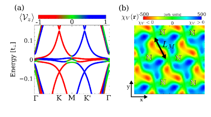
Figure 6: (a) Band structure in the presence of a N impurity, and (b) valley current at charge neutrality. It is observed that, although the presence of a dopand creates a non-zero intervalley scattering, the low-energy bands remain relatively flat. The emergence of intervalley scattering can be seen in the depletion of the bulk valley currents in (b). The valley flux in (b) is summed over the three layers. Calculations performed with tight-binding.

We now consider the effect of a chemical impurity in the tight-binding model. We model the addition of a chemical impurity by adding to the Hamiltonian $\mathcal{H}_{D}=w\sum_{s}c^{\dagger}_{i,s}c_{i,s}$, where $i$ in the site that has been chemically replaced. We take $w=-2t$, which is the typical energy scale expected for a $N$ dopand, and yields results comparable with the first principle calculations. For the sake of concreteness we will focus on the case with interlayer bias, so our full Hamiltonian will be $\mathcal{H}=\mathcal{H}_{0}+\mathcal{H}_{V}+\mathcal{H}_{D}$. With the previous Hamiltonian, we now compute the electronic band structure and project each eigenstate onto the valley operator. The result is shown in Fig. 6a, where we see that small anticrossings appear as in the first-principles calculations. The valley projection clearly shows that such anticrossings are associated with intervalley mixing. The effect of the impurity in terms of intervalley mixing can also be readily seen in the bulk valley currents. In particular, the existence of the impurity is expected to strongly perturb the original valley fluxes in the unit cell, depleting the local value of the valley Chern number. This is verified in Fig. 6b, where we observe that the original valley fluxes are impacted by the presence of the impurity.

Interestingly, despite the effect in terms of intervalley mixing, the low-energy bands remain relatively flat, retaining their associated large density of states. This suggests that correlated states can still appear in chemical doped twisted trilayers. It is worth to emphasize that despite this large density of states, correlated phases relying on valley coherent states will be strongly suppressed due to the impurity-induced intervalley mixing. In particular, valley ferromagnet states, and valley triplet superconducting states will be depleted due to chemical dopands. Nevertheless, conventional spin-singlet valley-singlet states are not affected by the presence of intervalley scattering. Motivated by this, in the next section we address the emergence of spin/valley singlet superconductivity, and show how the superfluid density impacts the high energy dispersive states.

V Superconducting state

The large density of states close to charge neutrality suggests that the twisted graphene trilayer can have superconducting instabilities, similarly to twisted bilayers and tetra-layers. As shown above, both with electrostatic and chemical doping the system shows divergent density of state close to charge neutrality. For the sake of concreteness we will now focus on the electrostatically doped system, yet we have verified that our results remain qualitatively unchanged with chemical doping.

An emergent superconducting state is associated with a Fermi surface instability, yet its effect can give rise to second order perturbations above the Fermi energy. In order to understand the potential impact at high-energies, we first briefly analyze the structure of the low-energy states. This can be done by comparing the spatial distribution of the low-energy states with respect to the Fermi surface states. In particular, we define the projection over the Fermi surface states as $\mathcal{R}=\int d^{2}\mathbf{r}|\Psi(\mathbf{r})|^{2}\rho_{F}(\mathbf{r})$ with $\rho_{F}(\mathbf{r})$ the local density at the Fermi energy $\rho_{F}(\mathbf{r})\sim\int\langle\mathbf{r}|\delta(E_{F}-H)|\mathbf{r}\rangle$. The quantity $\mathcal{R}$ allows to qualitatively distinguish which states are localized in the same region at the Fermi surface states.

By computing the Fermi surface state projector $\mathcal{R}$, it observed that the states of the flat band are localized in similar regions. In contrast, as one departs from the Fermi energy, the states start to delocalize to other regions of the unit cell (Fig. 7a). This highlights the different orbital nature of the nearly flat bands (in purple) and low-energy dispersive bands (in green). Importantly, and in strike contrast with twisted graphene bilayers, the flat bands of this system are not decoupled from the dispersive states, suggesting that the superconducting states of this system will have a genuine multiorbital nature.

Given the unavoidable entanglement between the flat and dispersive bands, an effective model description of this twisted trilayer cannot be easily performed. Therefore, in the following we will study the emergent superconducting state by exploiting the full atomistic model, including all the bands in our calculation. A variety of mechanisms have been suggested to give rise to attractive interactions in these systems, including phonon,Peltonen et al. (2018); Wu et al. (2018); Lian et al. (2019) CoulombGonzález and Stauber (2019) and magnon fluctuations.Xu and Balents (2018); Liu et al. (2018) For the sake of concreteness, we will focus on effective local attractive interactions, as employed in other twisted graphene systems Zhao and Paramekanti (2006); Uchoa and Castro Neto (2007); Kopnin and Sonin (2008); Julku et al. (2020); Heikkilä and Hyart (2019); Peltonen et al. (2018); Wu et al. (2018); Hu et al. (2019)

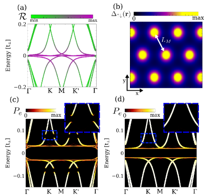
Figure 7: Normal state band structure (a) in the absence of interactions, with the color denoting the projection of the states on the density of states at the Fermi energy. Upon introducing interactions, a non-zero superfluid density appears as shown in panel (b). Panel (c) shows the associated electronic dispersion (c) to the selfconsistent solution of (b), where we have projected the eigenstates over the the electron sector. Panel (d) shows the electronic dispersion projected in the electron sector for a uniform superfluid density, highlighting that the high energy anticrossings stem from the non-uniform pairing. Calculations performed with tight-binding.

$$\mathcal{H}_{I}=-\sum_{i}gc_{i,\uparrow}^{\dagger}c_{i,\uparrow}c_{i,\downarrow}^{\dagger}c_{i,\downarrow}$$ (4)

that we solve at the mean field level $\mathcal{H}_{I}^{MF}=-g\sum_{i}\langle c_{i,\uparrow}^{\dagger}c_{i,\downarrow}^{\dagger}\rangle c_{i,\uparrow}c_{i,\downarrow}+h.c.$ where $\langle c_{i,\uparrow}^{\dagger}c_{i,\downarrow}^{\dagger}\rangle$ is computed self-consistently for the full Hamiltonian $\mathcal{H}=\mathcal{H}_{0}+\mathcal{H}_{V}+\mathcal{H}^{MF}_{I}$, that we solve with the Bogoliubov-de Gennes (BdG) formalism. The local attractive interaction $g$ will give rise to a net superfluid density, with a moiré momentum structure of $s$-wave symmetry. In the following we take $g=t$, and we verified that our results remain qualitatively similar with smaller interaction strengths. We note that although interactions are local, the would lead to a non-trivial multiorbital structural in the moiré orbital space.

By solving the previous selfconsistent problem, we find that the superfluid density is non-uniform in the moiré unit cell (Fig. 7b), stemming from the non-uniformity of the low-energy states. By projecting the BdG eigenstates in the electron sector via the electron projector $P_{e}$, we observe that the net non-uniform superfluid density $\Delta_{\uparrow\downarrow}(\mathbf{r}_{i})\sim\langle c^{\dagger}_{i,\uparrow}c^{\dagger}_{i,\downarrow}\rangle$ gives rise to a full gap in the Brillouin zone in the superconducting state. This phenomenology is similar to the one found in twisted graphene bilayers. More interestingly, besides the gap opening at the chemical potential, anticrossings appear in high energy bands when the selfconsistent pairing is included (Fig. 7c). It is worth to emphasize that, in the presence of a uniform pairing artificially imposed, the high energy anticrossings disappear, leading only to the gap opening at charge neutrality (Fig. 7d). The emergence of gap openings away from charge neutrality is associated to the intrinsically multiorbital nature of the superconducting state, and stems from the non-unitarity of the superconducting matrix in orbital subspace.Lado and Sigrist (2019); Zaki et al. (2019) Interestingly, this shows that signatures of the superconducting state can be obtained by analyzing the system away from the chemical potential, and could provide powerful spectroscopic signaturesAmorim (2018); Lisi et al. (2020) of the superconducting state.

VI Conclusions

By combining first-principles calculation and low-energy effective models, we have shown that twisted graphene trilayers realize tunable electronic systems. In particular, is was shown that nearly perfect flat bands can be electrically controlled, that coexist with highly dispersive states. Interestingly, such electric flattening of the bands is accompanied by the emergence of bulk valley currents. We have found both from first principles and low-energy calculations that chemical doping does not destroy the flat bands, yet it substantially impacts the bulk valley currents. This suggests that chemical doping of twisted graphene trilayers could provide an intrinsic way of providing the necessary electronic doping required for the emergence of a superconducting state. We finally demonstrated that an emergent superconducting state would give rise to spectroscopic changes int he high energy bands, associated to the non-uniform superfluid density. Our results highlight the rich physics of twisted graphene trilayers, and provide a starting point to explore the interplay between flat bands, correlation and dispersive states in twisted graphene multilayers.

Appendix

Appendix A First-principles calculations

Description of the coupling between the graphene layers was conducted through self-consistent calculations with the SIESTA codeSoler et al. (2002) within a localized orbital basis set scheme. Paramagnetic calculations were conducted using a double-$\zeta$ basis set, and the local density approximation (LDA) approachKohn and Sham (1965) for the exchange-correlation functional was used. Atomic positions of systems formed by over 5514 atoms were fully relaxed with a force tolerance of 0.02 eV/Å. The integration over the Brillouin zone (BZ) was performed using a Monkhorst sampling in $\Gamma$ point. The radial extension of the orbitals had a finite range with a kinetic energy cutoff of 50 meV. A vertical separation of 35 Å in the simulation box prevents virtual periodic parallel layers from interacting.

Appendix B The valley operator

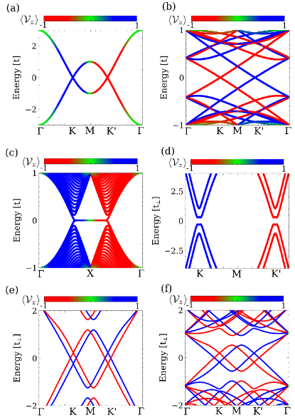
Figure 8: Valley expectation value for the minimal unit cell of a honeycomb lattice (a) and in an 8x8 supercell. Panel (c) shows the projection of the valley operator on the states of a graphene zigzag ribbon, and panel (d) on a biased aligned Bernal stacked graphene bilayer. Panels (e,f) show the projection of the valley operator for a biased twisted graphene bilayer, for a rotation angle of 10^∘ in (e) and 5^∘ in (f). We took $V=0.05t$ for (d,e,f).

Valley is an emergent quantum number in graphene, and as a result, it is not apparent how a valley operator can be described in a real space tight-binding basis. A simple procedure to define the valley expectation value in a tight binding model is by noting that for the z-component of the valley, we are looking for an operator with eigenvalue +1 for states in one valley, and -1 for states in another valley. This would be accomplished by a Hamiltonian that realizes a valley-dependent chemical potential. Let us first focus in a honeycomb lattice, and let us take the following real space operator in a honeycomb latticeColomés and Franz (2018); Ramires and Lado (2018, 2019)

$$\mathcal{V}_{z}=\frac{i}{3\sqrt{3}}\sum_{\langle\langle i,j\rangle\rangle,s}\eta_{ij}\sigma_{z}^{ij}c^{\dagger}_{i,s}c_{j,s},$$ (5)

where $\langle\langle i,j\rangle\rangle$ denotes second neighbor sites, $\eta_{ij}=\pm 1$ for clockwise or anticlockwise hopping, and $\sigma^{ij}_{z}$ is a Pauli matrix associated with the sublattice degree of freedom. The previous operator is diagonal in sublattice, and is proportional to the identity matrix in reciprocal space $\begin{pmatrix}f(\mathbf{k})&0\\ 0&f(\mathbf{k})\\ \end{pmatrix}$ with $f(\mathbf{k})$ the Fourier transform of the real-space hopping. It is easily shown that $f(\mathbf{k})\approx+1$ close to the K-point, and $f(\mathbf{k})\approx-1$ close the K’-point, and as a result such second neighbor hopping allows to compute the expectation value of the valley for a specific state. In particular, by taking the expectation value $\langle\mathcal{V}_{z}\rangle=\langle\Psi|\mathcal{V}_{z}|\Psi\rangle$, we will obtain $\langle\mathcal{V}_{z}\rangle\approx 1$ if $\Psi$ is a state belonging to valley K, and $\langle\mathcal{V}_{z}\rangle\approx-1$ if $\Psi$ is a state belonging to valley K’. This can be clearly seen in Fig. 8a, where we show the valley expectation value for the states of the honeycomb lattice, showing that the states around valley K have eigenvalue +1, and around K’ eigenvalue -K’.

The valley operator allows us to easily track the valley flavor of the electronic states in various situations. Let us now show some of them for the sake of clarity. The simplest case consists of the electronic structure of a supercell of a honeycomb lattice. In particular, we show in Fig. 8b the bandstructure for 8x8 supercell, indicating that the valley operator allows following the original valley flavor of the states in the folded band structure. It is worth to note that such operator can be defined in a graphene structure, without requiring two-dimensional periodicity, for example for graphene nanoribbons. In particular, we show in 8c the band-structure of a zigzag graphene nanoribbon, demonstrating that the valley operator correctly identifies the valley flavor of each state.

The valley operator can be easily extended to graphene multilayers. In particular, by defining the valley operator of layer $\alpha$ as $\mathcal{V}^{\alpha}_{z}$, the total valley operator is defined as $\mathcal{V}_{z}=\sum_{\alpha}\mathcal{V}^{\alpha}_{z}$. Let us first illustrate this with a simple graphene multilayer, an electrically biased Bernal stacked graphene bilayer. In this situation shown in Fig. 8d, we again observe that the multilayer valley operator correctly identifies the states belonging to the different valleys. This very same idea can be used for twisted graphene multilayers. In particular, in Fig. 8ef we show that in a biased twisted graphene bilayer at an angle of 10 degrees (Fig. 8e) and 5 degrees (Fig. 8f), the valley operator correctly identifies the microscopic valley of each state.

Appendix C Origin of the high energy anticrossings in the superconducting state

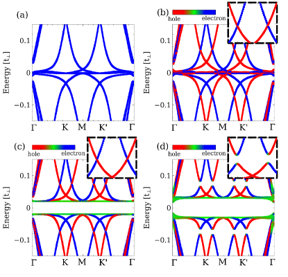
Figure 9: Band structure of the biased twisted trilayer in the normal state, showing only the electron sector (a) and both the BdG electron and hole sectors (b). When a non-zero superfluid weight is included, anticrossings in the high energy bands do not appear for a uniform superfluid matrix $\Delta\sim\mathcal{I}$ (c). In contrast, anticrossings at high energies emerge for a self-consistent non-uniform superfluid weight (d), due to the non-zero matrix element $\Gamma=\langle\Psi_{n,\mathbf{k}}|\hat{\Delta}|\Psi_{l,\mathbf{-k}}\rangle\neq 0$

In the following, we elaborate on the origin of the high energy anticrossings in the superconducting state. Let us start with the band structure of the biased twisted trilayer graphene, as shown in Fig. 9a. By extending the spectra in a Bogoliubov de Gennes formalism, hole replicas of the original states appear. This is shown in Fig. 9b for $\Delta=0$, where the blue bands denote electron-like bands, and red bands denote the hole replicas. It is worth to note that in this situation, electron-like and hole-like bands above the chemical potential cross, and therefore a non-zero superfluid weight can potentially lead to anticrossings, as such terms couples electron and hole sectors. Let us now turn on a spatially uniform superfluid weight, as shown in Fig. 9c. In this situation, it is observed that for the electron and hole-like bands cross above the chemical potential no anticrossings appears. The coupling between the electron and hole states above the chemical potential is proportional to the overlap of the single particle wavefunction $\Psi_{n,\mathbf{k}}$ with the superconducting matrix $\hat{\Delta}$, and takes the form $\Gamma=\langle\Psi_{n,\mathbf{k}}|\hat{\Delta}|\Psi_{l,\mathbf{-k}}\rangle$ with $n\neq l$. For uniform superfluid density $\hat{\Delta}\sim\mathcal{I}$ with $\mathcal{I}$ the identity matrix, we have $\Gamma=0$ from the orthogonality of the wavefunctions, and therefore no anticrossings appear in the high energy bands of Fig. 9c. In stark contrast, when the superfluid weight is non-uniform in space we have $\hat{\Delta}\not\propto\mathcal{I}$, we generically have $\Gamma=\langle\Psi_{n,\mathbf{k}}|\hat{\Delta}|\Psi_{l,\mathbf{-k}}\rangle\neq 0$, leading to an effective anticrossing between the states. As a result, the appearance of anticrossing in the high energy bands is a direct consequence of the non-uniform superfluid weight. We finally note that this argument relies on the original time-reversal symmetry of the twisted trilayer graphene Hamiltonian.

References

- Cao et al. (2018) Y. Cao, V. Fatemi, S. Fang, K. Watanabe, T. Taniguchi, E. Kaxiras, and P. Jarillo-Herrero, Nature 556, 43 (2018).
- Yankowitz et al. (2019) M. Yankowitz, S. Chen, H. Polshyn, Y. Zhang, K. Watanabe, T. Taniguchi, D. Graf, A. F. Young, and C. R. Dean, Science 363, 1059 (2019).
- Liu et al. (2014) K. Liu, L. Zhang, T. Cao, C. Jin, D. Qiu, Q. Zhou, A. Zettl, P. Yang, S. G. Louie, and F. Wang, Nature Communications 5 (2014), 10.1038/ncomms5966.
- Lu et al. (2019) X. Lu, P. Stepanov, W. Yang, M. Xie, M. A. Aamir, I. Das, C. Urgell, K. Watanabe, T. Taniguchi, G. Zhang, A. Bachtold, A. H. MacDonald, and D. K. Efetov, Nature 574, 653 (2019).
- Rickhaus et al. (2018) P. Rickhaus, J. Wallbank, S. Slizovskiy, R. Pisoni, H. Overweg, Y. Lee, M. Eich, M.-H. Liu, K. Watanabe, T. Taniguchi, T. Ihn, and K. Ensslin, Nano Letters 18, 6725 (2018).
- San-Jose and Prada (2013) P. San-Jose and E. Prada, Phys. Rev. B 88, 121408 (2013).
- Liao et al. (2020) M. Liao, Z. Wei, L. Du, Q. Wang, J. Tang, H. Yu, F. Wu, J. Zhao, X. Xu, B. Han, K. Liu, P. Gao, T. Polcar, Z. Sun, D. Shi, R. Yang, and G. Zhang, Nature Communications 11 (2020), 10.1038/s41467-020-16056-4.
- Shimazaki et al. (2020) Y. Shimazaki, I. Schwartz, K. Watanabe, T. Taniguchi, M. Kroner, and A. Imamoğlu, Nature 580, 472 (2020).
- Lopes dos Santos et al. (2007) J. M. B. Lopes dos Santos, N. M. R. Peres, and A. H. Castro Neto, Phys. Rev. Lett. 99, 256802 (2007).
- Suárez Morell et al. (2010) E. Suárez Morell, J. D. Correa, P. Vargas, M. Pacheco, and Z. Barticevic, Phys. Rev. B 82, 121407 (2010).
- Serlin et al. (2019) M. Serlin, C. L. Tschirhart, H. Polshyn, Y. Zhang, J. Zhu, K. Watanabe, T. Taniguchi, L. Balents, and A. F. Young, Science 367, 900 (2019).
- Ahn et al. (2018) S. J. Ahn, P. Moon, T.-H. Kim, H.-W. Kim, H.-C. Shin, E. H. Kim, H. W. Cha, S.-J. Kahng, P. Kim, M. Koshino, Y.-W. Son, C.-W. Yang, and J. R. Ahn, Science 361, 782 (2018).
- Moon et al. (2019) P. Moon, M. Koshino, and Y.-W. Son, Phys. Rev. B 99, 165430 (2019).
- Yu et al. (2019) G. Yu, Z. Wu, Z. Zhan, M. I. Katsnelson, and S. Yuan, npj Computational Materials 5 (2019), 10.1038/s41524-019-0258-0.
- Pezzini et al. (2020) S. Pezzini, V. Miseikis, G. Piccinini, S. Forti, S. Pace, R. Engelke, F. Rossella, K. Watanabe, T. Taniguchi, P. Kim, and C. Coletti, arXiv e-prints , arXiv:2001.10427 (2020), arXiv:2001.10427 [cond-mat.mes-hall] .
- Chen et al. (2020) S. Chen, M. He, Y.-H. Zhang, V. Hsieh, Z. Fei, K. Watanabe, T. Taniguchi, D. H. Cobden, X. Xu, C. R. Dean, and M. Yankowitz, arXiv e-prints , arXiv:2004.11340 (2020), arXiv:2004.11340 [cond-mat.mes-hall] .
- Polshyn et al. (2020) H. Polshyn, J. Zhu, M. A. Kumar, Y. Zhang, F. Yang, C. L. Tschirhart, M. Serlin, K. Watanabe, T. Taniguchi, A. H. MacDonald, and A. F. Young, arXiv e-prints , arXiv:2004.11353 (2020), arXiv:2004.11353 [cond-mat.str-el] .
- Castro et al. (2007) E. V. Castro, K. S. Novoselov, S. V. Morozov, N. M. R. Peres, J. M. B. L. dos Santos, J. Nilsson, F. Guinea, A. K. Geim, and A. H. C. Neto, Phys. Rev. Lett. 99, 216802 (2007).
- Liu et al. (2019) X. Liu, Z. Hao, E. Khalaf, J. Y. Lee, K. Watanabe, T. Taniguchi, A. Vishwanath, and P. Kim, arXiv e-prints , arXiv:1903.08130 (2019), arXiv:1903.08130 [cond-mat.mes-hall] .
- Shen et al. (2020) C. Shen, Y. Chu, Q. Wu, N. Li, S. Wang, Y. Zhao, J. Tang, J. Liu, J. Tian, K. Watanabe, T. Taniguchi, R. Yang, Z. Y. Meng, D. Shi, O. V. Yazyev, and G. Zhang, Nature Physics (2020), 10.1038/s41567-020-0825-9.
- Ramires and Lado (2018) A. Ramires and J. L. Lado, Phys. Rev. Lett. 121, 146801 (2018).
- Wolf et al. (2019a) T. M. R. Wolf, J. L. Lado, G. Blatter, and O. Zilberberg, Phys. Rev. Lett. 123, 096802 (2019a).
- Abouelkomsan et al. (2020) A. Abouelkomsan, Z. Liu, and E. J. Bergholtz, Phys. Rev. Lett. 124, 106803 (2020).
- Liu et al. (2020) Z. Liu, A. Abouelkomsan, and E. J. Bergholtz, arXiv e-prints , arXiv:2004.09522 (2020), arXiv:2004.09522 [cond-mat.mes-hall] .
- Repellin and Senthil (2019) C. Repellin and T. Senthil, arXiv e-prints , arXiv:1912.11469 (2019), arXiv:1912.11469 [cond-mat.str-el] .
- Ledwith et al. (2019) P. J. Ledwith, G. Tarnopolsky, E. Khalaf, and A. Vishwanath, arXiv e-prints , arXiv:1912.09634 (2019), arXiv:1912.09634 [cond-mat.str-el] .
- Carr et al. (2018) S. Carr, D. Massatt, S. B. Torrisi, P. Cazeaux, M. Luskin, and E. Kaxiras, Phys. Rev. B 98, 224102 (2018).
- Lin et al. (2018) X. Lin, D. Liu, and D. Tománek, Phys. Rev. B 98, 195432 (2018).
- Nam and Koshino (2017) N. N. T. Nam and M. Koshino, Phys. Rev. B 96, 075311 (2017).
- Leconte et al. (2019) N. Leconte, S. Javvaji, J. An, and J. Jung, arXiv e-prints , arXiv:1910.12805 (2019), arXiv:1910.12805 [cond-mat.mes-hall] .
- Brihuega and Yndurain (2017) I. Brihuega and F. Yndurain, The Journal of Physical Chemistry B 122, 595 (2017).
- Koshino and Son (2019) M. Koshino and Y.-W. Son, Phys. Rev. B 100, 075416 (2019).
- Angeli et al. (2019) M. Angeli, E. Tosatti, and M. Fabrizio, Phys. Rev. X 9, 041010 (2019).
- Rickhaus et al. (2019) P. Rickhaus, G. Zheng, J. L. Lado, Y. Lee, A. Kurzmann, M. Eich, R. Pisoni, C. Tong, R. Garreis, C. Gold, M. Masseroni, T. Taniguchi, K. Wantanabe, T. Ihn, and K. Ensslin, Nano Letters 19, 8821 (2019).
- Ochoa (2019) H. Ochoa, Phys. Rev. B 100, 155426 (2019).
- Suárez Morell et al. (2013) E. Suárez Morell, M. Pacheco, L. Chico, and L. Brey, Phys. Rev. B 87, 125414 (2013).
- Li et al. (2019) X. Li, F. Wu, and A. H. MacDonald, arXiv e-prints , arXiv:1907.12338 (2019), arXiv:1907.12338 [cond-mat.mtrl-sci] .
- Khalaf et al. (2019) E. Khalaf, A. J. Kruchkov, G. Tarnopolsky, and A. Vishwanath, Phys. Rev. B 100, 085109 (2019).
- Carr et al. (2019) S. Carr, C. Li, Z. Zhu, E. Kaxiras, S. Sachdev, and A. Kruchkov, arXiv e-prints , arXiv:1907.00952 (2019), arXiv:1907.00952 [cond-mat.str-el] .
- Mora et al. (2019) C. Mora, N. Regnault, and B. A. Bernevig, Phys. Rev. Lett. 123, 026402 (2019).
- Park et al. (2020) Y. Park, B. Lingam Chittari, and J. Jung, arXiv e-prints , arXiv:2005.01258 (2020), arXiv:2005.01258 [cond-mat.mes-hall] .
- Bistritzer and MacDonald (2011) R. Bistritzer and A. H. MacDonald, Proceedings of the National Academy of Sciences 108, 12233 (2011).
- Angeli et al. (2018) M. Angeli, D. Mandelli, A. Valli, A. Amaricci, M. Capone, E. Tosatti, and M. Fabrizio, Phys. Rev. B 98, 235137 (2018).
- Lucignano et al. (2019) P. Lucignano, D. Alfè, V. Cataudella, D. Ninno, and G. Cantele, Phys. Rev. B 99, 195419 (2019).
- Cantele et al. (2020) G. Cantele, D. Alfè, F. Conte, V. Cataudella, D. Ninno, and P. Lucignano, arXiv e-prints , arXiv:2004.14323 (2020), arXiv:2004.14323 [cond-mat.mtrl-sci] .
- Haddadi et al. (2020) F. Haddadi, Q. Wu, A. J. Kruchkov, and O. V. Yazyev, Nano Letters 20, 2410 (2020).
- Kim et al. (2016) K. Kim, M. Yankowitz, B. Fallahazad, S. Kang, H. C. P. Movva, S. Huang, S. Larentis, C. M. Corbet, T. Taniguchi, K. Watanabe, S. K. Banerjee, B. J. LeRoy, and E. Tutuc, Nano Letters 16, 1989 (2016).
- Note (1) At low energies the spectra is invariant upon rescaling of the interlayer coupling, which allows to explore effective smaller angles with smaller unit cells.Su and Lin (2018); Gonzalez-Arraga et al. (2017) Our calculations are performed with a resscaled .
- Culchac et al. (2019) F. J. Culchac, R. B. Capaz, L. Chico, and E. Suarez Morell, arXiv e-prints , arXiv:1911.01347 (2019), arXiv:1911.01347 [cond-mat.mes-hall] .
- Morell et al. (2015) E. S. Morell, P. Vargas, P. Häberle, S. A. Hevia, and L. Chico, Phys. Rev. B 91, 035441 (2015).
- Ramires and Lado (2019) A. Ramires and J. L. Lado, Phys. Rev. B 99, 245118 (2019).
- Lopez-Bezanilla and Lado (2019) A. Lopez-Bezanilla and J. L. Lado, Phys. Rev. Materials 3, 084003 (2019).
- Lopes dos Santos et al. (2012) J. M. B. Lopes dos Santos, N. M. R. Peres, and A. H. Castro Neto, Phys. Rev. B 86, 155449 (2012).
- Colomés and Franz (2018) E. Colomés and M. Franz, Phys. Rev. Lett. 120, 086603 (2018).
- Wolf et al. (2019b) T. M. R. Wolf, J. L. Lado, G. Blatter, and O. Zilberberg, Phys. Rev. Lett. 123, 096802 (2019b).
- Manesco et al. (2020) A. L. R. Manesco, J. L. Lado, E. V. Ribeiro, G. Weber, and J. Rodrigues, Durval, arXiv e-prints , arXiv:2003.05163 (2020), arXiv:2003.05163 [cond-mat.mes-hall] .
- McCann (2006) E. McCann, Phys. Rev. B 74, 161403 (2006).
- Martin et al. (2008) I. Martin, Y. M. Blanter, and A. F. Morpurgo, Phys. Rev. Lett. 100, 036804 (2008).
- Zhang et al. (2013) F. Zhang, A. H. MacDonald, and E. J. Mele, Proceedings of the National Academy of Sciences 110, 10546 (2013).
- Mañes et al. (2007) J. L. Mañes, F. Guinea, and M. A. H. Vozmediano, Phys. Rev. B 75, 155424 (2007).
- San-Jose et al. (2012) P. San-Jose, J. González, and F. Guinea, Phys. Rev. Lett. 108, 216802 (2012).
- Ren et al. (2016) Y. Ren, Z. Qiao, and Q. Niu, Reports on Progress in Physics 79, 066501 (2016).
- Castro Neto et al. (2009) A. H. Castro Neto, F. Guinea, N. M. R. Peres, K. S. Novoselov, and A. K. Geim, Rev. Mod. Phys. 81, 109 (2009).
- Chen and Lee (2011) K.-T. Chen and P. A. Lee, Phys. Rev. B 84, 205137 (2011).
- Tkachov and Hentschel (2012) G. Tkachov and M. Hentschel, Phys. Rev. B 86, 205414 (2012).
- Yan et al. (2016) B. Yan, Q. Han, Z. Jia, J. Niu, T. Cai, D. Yu, and X. Wu, Phys. Rev. B 93, 041407 (2016).
- Rodrigues (2016) J. N. B. Rodrigues, Phys. Rev. B 94, 134201 (2016).
- Cea et al. (2019) T. Cea, N. R. Walet, and F. Guinea, Phys. Rev. B 100, 205113 (2019).
- Guinea and Walet (2018) F. Guinea and N. R. Walet, Proceedings of the National Academy of Sciences 115, 13174 (2018).
- Pantaleon et al. (2020) P. A. Pantaleon, T. Cea, R. Brown, N. R. Walet, and F. Guinea, arXiv e-prints , arXiv:2003.05050 (2020), arXiv:2003.05050 [cond-mat.str-el] .
- Goodwin et al. (2020) Z. A. H. Goodwin, V. Vitale, X. Liang, A. A. Mostofi, and J. Lischner, arXiv e-prints , arXiv:2004.14784 (2020), arXiv:2004.14784 [cond-mat.mes-hall] .
- Brun et al. (2016) S. J. Brun, V. M. Pereira, and T. G. Pedersen, Phys. Rev. B 93, 245420 (2016).
- Wang and Pantelides (2011) B. Wang and S. T. Pantelides, Phys. Rev. B 83, 245403 (2011).
- Liu et al. (2011) H. Liu, Y. Liu, and D. Zhu, J. Mater. Chem. 21, 3335 (2011).
- Lopez-Bezanilla et al. (2009a) A. Lopez-Bezanilla, F. Triozon, and S. Roche, Nano Letters 9, 2537 (2009a).
- Agnoli and Favaro (2016) S. Agnoli and M. Favaro, Journal of Materials Chemistry A 4, 5002 (2016).
- Georgakilas et al. (2012) V. Georgakilas, M. Otyepka, A. B. Bourlinos, V. Chandra, N. Kim, K. C. Kemp, P. Hobza, R. Zboril, and K. S. Kim, Chemical Reviews 112, 6156 (2012).
- Si et al. (2012) C. Si, W. Duan, Z. Liu, and F. Liu, Phys. Rev. Lett. 109, 226802 (2012).
- Pi et al. (2010) K. Pi, W. Han, K. M. McCreary, A. G. Swartz, Y. Li, and R. K. Kawakami, Phys. Rev. Lett. 104, 187201 (2010).
- Lopez-Bezanilla et al. (2009b) A. Lopez-Bezanilla, F. Triozon, S. Latil, X. Blase, and S. Roche, Nano Letters 9, 940 (2009b).
- Altland (2006) A. Altland, Phys. Rev. Lett. 97, 236802 (2006).
- Yang et al. (2019) H. Yang, Z.-Q. Gao, and F. Wang, arXiv e-prints , arXiv:1908.09555 (2019), arXiv:1908.09555 [cond-mat.supr-con] .
- Peltonen et al. (2018) T. J. Peltonen, R. Ojajärvi, and T. T. Heikkilä, Phys. Rev. B 98, 220504 (2018).
- Wu et al. (2018) F. Wu, A. H. MacDonald, and I. Martin, Phys. Rev. Lett. 121, 257001 (2018).
- Lian et al. (2019) B. Lian, Z. Wang, and B. A. Bernevig, Phys. Rev. Lett. 122, 257002 (2019).
- González and Stauber (2019) J. González and T. Stauber, Phys. Rev. Lett. 122, 026801 (2019).
- Xu and Balents (2018) C. Xu and L. Balents, Phys. Rev. Lett. 121, 087001 (2018).
- Liu et al. (2018) C.-C. Liu, L.-D. Zhang, W.-Q. Chen, and F. Yang, Phys. Rev. Lett. 121, 217001 (2018).
- Zhao and Paramekanti (2006) E. Zhao and A. Paramekanti, Phys. Rev. Lett. 97, 230404 (2006).
- Uchoa and Castro Neto (2007) B. Uchoa and A. H. Castro Neto, Phys. Rev. Lett. 98, 146801 (2007).
- Kopnin and Sonin (2008) N. B. Kopnin and E. B. Sonin, Phys. Rev. Lett. 100, 246808 (2008).
- Julku et al. (2020) A. Julku, T. J. Peltonen, L. Liang, T. T. Heikkilä, and P. Törmä, Phys. Rev. B 101, 060505 (2020).
- Heikkilä and Hyart (2019) T. T. Heikkilä and T. Hyart, Europhysics News 50, 24 (2019).
- Hu et al. (2019) X. Hu, T. Hyart, D. I. Pikulin, and E. Rossi, Phys. Rev. Lett. 123, 237002 (2019).
- Lado and Sigrist (2019) J. L. Lado and M. Sigrist, Phys. Rev. Research 1, 033107 (2019).
- Zaki et al. (2019) N. Zaki, G. Gu, A. M. Tsvelik, C. Wu, and P. D. Johnson, arXiv e-prints , arXiv:1907.11602 (2019), arXiv:1907.11602 [cond-mat.supr-con] .
- Amorim (2018) B. Amorim, Phys. Rev. B 97, 165414 (2018).
- Lisi et al. (2020) S. Lisi, X. Lu, T. Benschop, T. A. de Jong, P. Stepanov, J. R. Duran, F. Margot, I. Cucchi, E. Cappelli, A. Hunter, A. Tamai, V. Kandyba, A. Giampietri, A. Barinov, J. Jobst, V. Stalman, M. Leeuwenhoek, K. Watanabe, T. Taniguchi, L. Rademaker, S. J. van der Molen, M. Allan, D. K. Efetov, and F. Baumberger, arXiv e-prints , arXiv:2002.02289 (2020), arXiv:2002.02289 [cond-mat.str-el] .
- Soler et al. (2002) J. M. Soler, E. Artacho, J. D. Gale, A. García, J. Junquera, P. Ordejón, and D. Sánchez-Portal, Journal of Physics: Condensed Matter 14, 2745 (2002).
- Kohn and Sham (1965) W. Kohn and L. J. Sham, Phys. Rev. 140, A1133 (1965).
- Su and Lin (2018) Y. Su and S.-Z. Lin, Phys. Rev. B 98, 195101 (2018).
- Gonzalez-Arraga et al. (2017) L. A. Gonzalez-Arraga, J. L. Lado, F. Guinea, and P. San-Jose, Phys. Rev. Lett. 119, 107201 (2017).