An Unsupervised Semantic Sentence Ranking Scheme for Text Documents

Abstract

This paper presents Semantic SentenceRank (SSR), an unsupervised scheme for automatically ranking sentences in a single document according to their relative importance. In particular, SSR extracts essential words and phrases from a text document, and uses semantic measures to construct, respectively, a semantic phrase graph over phrases and words, and a semantic sentence graph over sentences. It applies two variants of article-structure-biased PageRank to score phrases and words on the first graph and sentences on the second graph. It then combines these scores to generate the final score for each sentence. Finally, SSR solves a multi-objective optimization problem for ranking sentences based on their final scores and topic diversity through semantic subtopic clustering. An implementation of SSR that runs in quadratic time is presented, and it outperforms, on the SummBank benchmarks, each individual judge’s ranking and compares favorably with the combined ranking of all judges.

1 Introduction

Ranking sentences in a single document according to their relative importance plays a central role in various applications, including summary extraction from a given document (e.g., see [1]), structured-overview generation over a large corpus of documents [2], and layered reading for fast comprehension of a given document. The last application enables the reader to read a layer of the most important sentences first, then subsequent layers of next important sentences until the entire document is read. This application is aimed to facilitate faster reading for understanding.

There are supervised and unsupervised methods for ranking sentences. Most unsupervised methods use easy-to-compute counting features, such as TF-IDF (term frequency-inverse document frequency) [3] and co-occurrences of words [4]. Such approaches are domain and language independent, and are often preferred over other approaches. Not using semantic information in the context, these methods may only produce suboptimal sentence ranking. Other unsupervised algorithms that use semantic information include Semantic Role Labelling [5], WordNet [6], and Named Entity Recognition [7]. These methods, unfortunately, impose a common limitation of language dependence. In other words, using these algorithms for a given language requires software tools to provide the underlying semantic information for the language, which may not be available.

Supervised methods require labeled data to train models. Modern supervised methods that learn feature representations automatically using a deep neural network model rely on a significant amount of labeled texts (e.g., see [8]). Lacking training data is a major obstacle when developing a supervised sentence-ranking algorithm. The SummBank dataset [9] for evaluating sentence-ranking algorithms, for example, contains only 200 news articles, which is far from sufficient to train a deep neural network model. Other larger datasets sufficient to train neural networks for summarization, such as CNN/DailyMail, are still unsuitable to train models for ranking sentences, because they only provide a few human-written highlights as a summary for each document.

There are no datasets available at this time for other languages that are suitable for training sentence-ranking models. For example, for the Chinese language, the LSCTS [10] dataset consists of news articles and an average of 1 to 2 sentences written by human annotators as a summary for each article; and the NLPCC 2017 dataset also consists of news articles with a summary of upto 45 Chinese characters written by human annotators. These datasets cannot be used to train sentence-ranking models. Lacking training data for a particular language has hindered adaption of a good supervised model for one language to different languages.

These concerns suggest a direction of investigating unsupervised sentence-ranking algorithms using semantic features that can be computed readily for a given language. Word-embedding representations [11] and Word Mover’s Distance (WMD) [12], for example, are semantic features of this kind. A good word embedding representation provides useful semantic and syntactic information. Requiring only a large amount of unlabeled texts, it is straightforward to compute word embedding representations for any language using unlabeled out-of-band data such as Wikipedia dumps of the underlying language. WMD uses word embedding representations to measure semantic distance between two sentences, which can be used to measure their semantic similarity.

This paper presents an unsupervised semantic sentence-ranking scheme called Semantic SentenceRank (SSR) using semantic features at the word, phrase, and sentence levels. SSR uses phrase and word embedding representations and co-occurrences to construct a semantic phrase-word graph, scores words and phrases using a variant of article-structure-biased PageRank, adjusts scores using Solfplus elevation, and computes a normalized score for each sentence. SSR then constructs a semantic sentence graph using WMD, scores sentences using a variant of article-structure-based PageRank, combines these sentence scores to generate the final sentence scores, computes semantic subtopic clustering of sentences, and ranks sentences by solving a multi-objective 0-1 knapsack problem that maximizes the final scores of selected sentences and the diversity of subtopic coverage.

The major contributions of this paper are as follows:

1. Flexibility: SSR is an unsupervised scheme using semantic features that can be computed readily for any language.

2. Efficiency: SSR runs in quadratic time when using AutoPhrase [13] to extract phrases, Affinity Propagation [14] to generate semantic subtopic clusters for sentences, and a greedy algorithm to approximate the multi-objective 0-1 knapsack problem.

3. Accuracy: Running on the DUC-02 dataset [15], the aforementioned implementation of SSR outperforms all previous algorithms under the ROUGE measures. More significantly, on the SummBank dataset [9] , SSR outperforms each individual judge’s ranking and compares favorably with the combined sentence ranking of all judges.

The rest of the paper is organized as follows: Section 2 provides a brief overview of related work. SSR is presented in Section 3. Detail descriptions of the major components of SSR are presented in Sections 4–7. Implementations and evaluation results are presented in Section 8. Conclusions and final remarks are presented in Section 9.

2 Related work

Extractive summarization algorithms that can specify the number of sentences in a summary can be used to rank sentences, and vice versa.

2.1 Supervised methods

Supervised summarization methods can be categorized into two categories: sentence labeling and sentence scoring.

Supervised sentence-labeling methods assign a binary label to each sentence $S$ to indicate whether the summary to be produced should include $S$, where the number of sentences with a “yes” label is determined by the training data. These methods, while being extractive, cannot be used to rank sentences, for they have no control of the number of “yes” labels to be produced. Early sentence-labeling algorithms assign labels to each sentence independently trained on handcrafted features [16] such as thematic words and uppercase words. A sequential Hidden Markov Model [17] was devised to account for local relations between sentences using three handcrafted features. Recently, deep recurrent-neural-network models [18, 8, 19] were used to derive a meaningful representation of a document and carry out sequence labeling based on labels of previous sentences. Trained with cross-entropy loss, however, these models were redundancy-prone and tend to generate verbose summaries [20]. Supervised sentence-labeling methods also have the following two downsides. First, labeled datasets that are large enough to train a model may be hard to come by. Second, labeled datasets required to train a model that exist for one language may not exist for a different language, making it difficult to adapt a model to different languages.

Supervised sentence-scoring methods depend on the underlying similarity measure of a sentence in a document to a benchmark summary. For example, CNN-W2V [21] is a model that computes a ROUGE score for each sentence in a document using the corresponding summaries in a labeled data as references, and uses such scores as the ground truth to train a convolutional-neural-network model to score sentences independently of input documents. This means that the same sentence appearing in different documents always has the same score. This is problematic, for the same sentence in different documents is unlikely to be equally important. A more reasonable approach is to score sentences via global optimization by taking previously scored sentences and their scores into consideration. Refresh [20], for example, is a recent model in this direction. It scores a sentence using previously scored sentences and the summaries of the underlying document in a labeled dataset, where sentence scores are used as a reward function in the model.

No matter what the underlying method is, it is necessary to have a large labeled dataset to train a supervised neural network model. This necessity remains a major obstacle, for such a dataset may not exist for a given language.

2.2 Unsupervised methods

Unsupervised summarization methods exploit relations between words, as related words “promote” each other. For example, TextRank [4] and LexRank [22] each models a document as a sentence graph based on word relations, but they use only syntactic features. PageRank [23] is used to score words.

Other methods incorporate additional information for achieving a higher accuracy. UniformLink [24], for example, constructs a sentence graph on a set of similar documents, where a sentence is scored based on both of the in-document score and cross-document score. URank [25], on the other hand, uses a unified graph-based framework to study both single-document and multi-document summarization.

The quality of a summary may be improved using max-margin methods [26] or integer-linear programming (ILP) [27, parveen2015topical]. Among the previous algorithms, $CP_{3}$ [28] offers the highest ROUGE-1, ROUGE-2, and ROUGE-SU4 scores over DUC-02. It uses a bipartite graph to represent a document, and a different algorithm, Hyperlink-Induced Topic Search (HITS) [29], is used to score sentences. $CP_{3}$ treats the summarization problem as an ILP problem, which maximizes the sentence importance, non-redundancy, and coherence simultaneously. However, since solving ILP is NP-hard, obtaining an exact solution to an ILP problem is intractable.

It is worth noting that a recent unsupervised method [30], while not related to the problem studied in this paper, may provide new ideas. On a collection of consumer reviews on a particular product, the method generates an abstractive sentence as the main review point, and ranks sentences by the number of descendants in a discourse tree rooted on the main review point. It would be interesting to investigate if this method can be modified to rank sentences of a given document according to their relative importance.

Early unsupervised methods have two common downsides:

1. They don’t promote diversity. This is because the importance of sentences are based only on sentence scores, and so sentences of high scores representing the same subtopic may all be included in a summary, leaving no room to include sentences with lower scores but with different subtopics.

2. These methods do not used semantic features.

3 Semantic SentenceRank

To overcome the downsides of the existing methods (supervised or unsupervised), a better sentence-ranking algorithm should incorporate semantic features and topic diversity, and it should be unsupervised.

Let $D$ denote a document consisting of $n$ sentences indexed as $S_{1},S_{2},\ldots,S_{n}$ in the order they appear, each with a length $l_{i}$, along with a maximum length capacity $L$, where $l_{i}$ is the number of characters contained in $S_{i}$. Let $F_{s}(S_{i})$ and $F_{d}(D)$ denote a semantic sentence scoring function and a diversity coverage measure, respectively. Then the semantic sentence-ranking problem is modeled as follows:

maximize $$\sum_{i=1}^{n}F_{s}(S_{i})x_{i}\mbox{ and }F_{d}(D),$$

subject to $$\sum\limits_{i=1}^{n}l_{i}x_{i}\leq L\mbox{ and }x_{i}\in\{0,1\}.$$

where $x_{i}$ is a 0-1 variable such that $x_{i}=1$ if sentence $S_{i}$ is selected, and 0 otherwise. By setting $L$ appropriately from small to large, one can obtain from solving the optimization problem the first sentence, then the second, then the third, and so on until all sentences are ranked. Unfortunately, this problem is NP-hard and so an approximation algorithm is needed.

SSR computes $F_{s}$ by combining salience scores at three levels: words, phrases, and sentences. In particular, it first constructs a semantic phrase-word graph (SPG) on phrases and words, and a semantic sentence graph (SSG) on sentences. It then computes $F_{d}$ using semantic subtopic clustering. Finally, SSR uses an

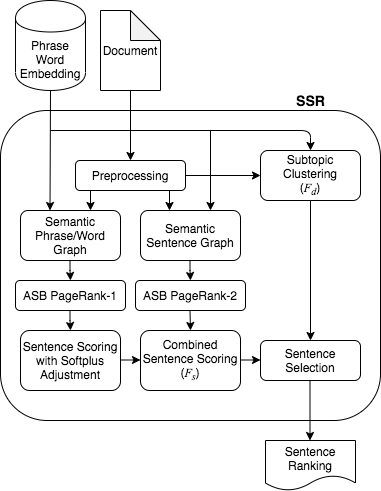
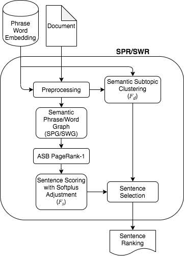
(a) Data flow diagram for SSR	(b) Data flow diagram for SPR/SWR

Figure 1: Major components of (a) SSR and (b) SPR/SWR

approximation algorithm based on $F_{s}$ and $F_{d}$ to rank sentences. Fig. 1(a) depicts the data flow diagram for the major components of SSR.

3.1 Sub-models

SSR contains two sub-models: one at the word level known as Semantic WordRank (SWR) [31], and one at the phrase-word level referred to as Semantic PhraseRank (SPR). In other words, SPR is SSR excluding semantic sentence graph and ABS-biased PageRank-2. Both SWR and SPR follow the same data follow diagram (see Fig. 1(b)), except that SWR does not consider phrase-level similarities. Both are faster than SSR, and perform well on selecting top-ranked sentences, which is sufficient for certain applications.

3.2 Phrase and word embedding

A searchable dataset of phrase and word embedding representations is calculated independently of SSR. Such an embedding dataset may be available for free download for some languages. If unavailable, it is straightforward to compute word and phrase embedding over an unlabeled Wikipedia dump using a standard method. To extract phrases, a linear-time unsupervised algorithm such as AutoPhrase [13] may be used. Recalculations of phrase and word embedding may be carried out once in a while on a larger Wikipedia dump.

3.3 Preprocessing

The preprocessing component computes, on a given document $D$, the phrases contained in $D$ using a phrase extractor, and the set of essential words contained in $D$ that, excluding these phrases, pass a part-of-speech (POS) filter, a stop-word filter, and a stemmer for reducing inflected words to the word stem. It removes all non-essential words. In what follows, unless otherwise stated, when words are mentioned, they are essential words.

Descriptions of the remaining components of SSR are presented in Sections 4–7.

4 Semantic graph representations

4.1 Semantic word graph

In addition to considering co-occurrence between words as in TextRank [4], the semantic word graph (SWG) for the underlying document adds embedding similarity of words to enhance connectivity of the graph. Adding semantic similarity is vital for processing analytic languages, such as Chinese, which seldom use inflections. When stemming is not applicable, semantic similarity serves as an alternative to represent the relations between words with similar meanings, allowing them to share the importance when computing PageRank scores for these nodes.

Let $G=(V,E)$ be a weighted graph of words in document $D$. Two words in $V$ are connected if either they co-occur within a window of $\Delta_{\text{SWG}}$ successive words in the document (e.g, $\Delta_{\text{SWG}}=2$), or the cosine similarity of their embedding representations exceeds a threshold value $\delta_{\text{SWG}}$ (e.g. $\delta_{\text{SWG}}=0.6$).

Let $u$ and $v$ be two adjacent nodes. For each edge $(u,v)$, if only one type of connection exists, then treat the weight of the other type 0. Assign the co-occurrence count of $u$ and $v$ as the initial weight to the co-occurrence connection and the cosine similarity value as the initial weight to the semantic connection. Normalize the initial weights of co-occurrence connections; namely, divide the initial co-occurrence weight by the total initial co-occurrence weight. Normalize the initial weights of semantic connections; namely, divide the initial semantic weight by the total initial semantic weight. Let $w_{c}(u,v)$ and $w_{s}(u,v)$ denote, respectively, the normalized weight for the co-occurrence connection and the semantic connection of $u$ and $v$. Finally, assign

$$w(u,v)=w_{c}(u,v)+w_{s}(u,v)$$

as the weight to the edge $(u,v)$.

4.2 Semantic phrase graph

In a SWG, words in a phrase (e.g., names, scientific terms, and general entity names) would have high co-occurrence counts if the phrase appears multiple times in the document. The meaning of a word inside a phrase may be different from that outside the phrase. For example, in the sentence “There is an apple on top of her Apple computer”, the word “Apple” appears outside and inside the phrase of “Apple computer”, which has different meanings. Thus, a high-quality phrase extractor is desired when building a phrase graph.

Given a document $D$, SSR applies a phrase extractor to segment phrases in $D$. Let $P$ denote the set of phrases and $W$ the set of words in $D$ after phrases are removed. If a phrase $p\in P$ of the given document does not appear in the database of phrases, then remove $p$ from $P$ and add the words $w\in p$ to $W$ (Note that the probability of this to happen is small if the construction of the database of phrase embedding uses the same phrase extractor.

A semantic phrase-word graph (SPG) is a weighted graph $(V,E)$ with $V=P\cup W$ such that two nodes are connected if either they co-occur in a small sliding window of $\Delta_{\text{SPG}}$ consecutive words and phrases or the cosine similarity of their embedding representations is greater than a threshold value $\delta_{\text{SPG}}$.

4.3 Semantic sentence graph

A semantic sentence graph (SSG) of a document $D$ is a weighted graph with sentences in $D$ being its nodes, where two sentences $S_{i}$ and $S_{j}$ are connected if either they contain a common word or phrase, or the WMD of $S_{i}$ and $S_{j}$ is below a certain value, which may be determined by how large a percentage of sentences should be connected. The weight of an edge $(S_{i},S_{j})$ is determined as follows:

1. Let $p_{ij}$ denote the number of phrases contained in both $S_{i}$ and $S_{j}$. After removing common phrases, let $v_{ij}$ denote the number of words contained in both $S_{i}$ and $S_{j}$. Let $|S_{i}|$ and $|S_{j}|$ denote, respectively, the number of words contained in $S_{i}$ and $S_{j}$. Let

   $$w_{c}(i,j)=\frac{p_{ij}+v_{ij}}{\log_{10}|S_{i}|+\log_{10}|S_{j}|}.$$

2. Define a different similarity measure of $S_{i}$ and $S_{j}$ by

   $$\text{sim}_{P}(S_{i},S_{j})=\frac{1}{1+\text{WMD}(S_{i},S_{j})}.$$ (1)

   Sort the similarity scores given by Eq. (1) in descending order. Select a $\Gamma\%$ of the edges with corresponding similarity scores being the top $\Gamma\%$ of the similarity scores (e.g., $\Gamma=30$). Add these semantic edges to the graph with weights being the corresponding similarity scores.

3. Normalize the co-occurrence edge weight $w_{c}(i,j)$; namely, divide $w_{c}(i,j)$ by $\sum_{i\not=j}w_{c}(i,j)$. Normalize the semantic edge weight; namely, divide the similarity given by Eq. (1) by the total similarity weight of all semantic edges. Sum up the two normalized weights to be the final edge weight $w_{ij}$.

5 Sentence scoring

5.1 Article-structure-biased PageRank-1

Article structures define how information is presented. For example, the typical structure of news articles is an inverted pyramid [32], where critical information is presented at the beginning, followed by additional information with less important details. In academic writing, the structure of an article would look like an hourglass, which includes an additional conclusion piece at the end of the article. Thus, sentence locations in an article according to the underlying structure also plays a role in ranking sentences. SWR uses a position-biased PageRank algorithm [33].

Directly applying PageRank, one can compute a score $W(v_{i})$ of a node $v_{i}\in G$ by iterating the following equation until converging:

$$W(v_{i})= d\bigg{(}\sum_{v_{j}\in Adj(v_{i})}\frac{w_{ji}}{\sum\limits_{v_{k}\in Adj(v_{j})}w_{jk}}W(v_{j})\bigg{)}+$$

$$+(1-d),$$ (2)

where $Adj(v_{i})$ denotes the set of nodes adjacent to $v_{i}$, $d\in(0,1)$ is a damping factor, and $w_{ji}$ is the weight of the edge between node $j$ and node $i$. The value of $d$ is set to 0.85 as in the original PageRank paper [34] and the TextRank paper [4]. The intuition behind this equation is that the importance of a node $v_{i}$ is affected by the scores of its adjacent nodes and the probability of $1-d$ for jumping from a random node to node $v_{i}$.

Eq. (2) is an unbiased PageRank, where each word is assumed equally likely to start from. In article-structure-biased (ASB) PageRank, each word $v_{i}$ is biased with a probability $P(v_{i})$ according to the underlying article structure. For example, in the inverted pyramid structure, a higher probability is assigned to a word that appears closer to the beginning of the article.

Rank the importance of sentence locations from the most important to the least important based on the underlying article structure (Note: This is not the sentence ranking to be computed). Let $\text{LS}_{i}(w)$ denote the location score of $w\in S_{i}$, where $S_{i}$ is the $i$-th sentence.

The probability for node $v_{i}$ can now be computed by

$$P(v_{i})=\frac{\sum_{k:v_{i}\in S_{k}}{\text{LS}_{k}(v_{i})}}{\sum_{j,k:v_{j}\in S_{k}}{\text{LS}_{k}(v_{j})}}.$$

Note that the above computation is at the sentence level, which can be easily adapted to the word level by ranking words instead of sentences.

The ASB PageRank score $W^{\prime}(v_{i})$ for node $v_{i}$ is computed as follows:

$$W^{\prime}(v_{i})= d\bigg{(}\sum_{v_{j}\in Adj(v_{i})}\frac{w_{ji}}{\sum_{v_{k}\in Adj(v_{j})}w_{jk}}W^{\prime}(v_{j})\bigg{)}+$$

$$+(1-d)P(v_{i}).$$ (3)

Computation starts with an arbitrary initial value for each node, and iterates the computation of Eq. (3) until it converges.

$W^{\prime}(v_{i})$, referred to as salient score, represents its importance relative to the other words in the document.

5.2 Softplus adjustment

Let $S$ be a sentence. To score $S$, one may simply sum up the salient score of each word contained in $S$ and normalize it by $|S|$ (the number of essential words contained in $S$). Normalization ensures that longer sentences and shorter sentences are comparable (otherwise, larger scores may have larger scores just because they have more words). Namely, let

$$\text{sal}(S)=\frac{1}{|S|}\sum_{v_{i}\in S}W^{\prime}(v_{i}).$$

This way of scoring, however, has a drawback. To see this, suppose that $S_{1}$ and $S_{2}$ are two sentences with similar scores under this method, and contain about the same number of words. If the distribution of word scores for words contained in $S_{1}$ follows the Pareto Principle, namely, a few words have very high scores and the rest have very low scores close to 0, while $S_{2}$ has roughly a uniform word score distribution, where the high scores of a few words in $S_{1}$ are much larger than the (almost uniform) scores of words in $S_{2}$, then the few words in $S_{1}$ with very high scores would make $S_{1}$ appear more important than $S_{2}$. Using direct summation of salient word scores, it is possible to end up with the opposite outcome.

Using the Softplus function $sp(x)=\ln(1+e^{x})$ helps overcome this drawback [35]. Commonly used as an activation function in neural networks, $sp(x)$ offers a significant elevation of $x$ when $x$ is a small positive number. If $x$ is large, then $sp(x)\approx x$.

Apply the Softplus function to each word, and sum up the elevated values to be the salient score of $S$, denoted by $\text{sal}_{sp}(S)$. Namely,

$$\text{sal}_{sp}(S)=\frac{1}{|S|}\sum_{v_{i}\in S}\ln(1+e^{W^{\prime}(v_{i})}).$$ (4)

To illustrate this using a numerical example, assume that $S_{1}$ and $S_{2}$ each consists of 5 words, with original scores ($W^{\prime}$) and Softplus scores ($sp^{\prime}=sp\circ W^{\prime}$) given in the following table (Table 1):

Table 1: Numerical examples with $W^{\prime}$ and $sp^{\prime}$ scores

$S_{1}$	$v_{11}$	$v_{12}$	$v_{13}$	$v_{14}$	$v_{15}$	sal
$W^{\prime}$	2.6	2.2	2.1	0.3	0.2	1.48
$sp^{\prime}$	2.67	2.31	2.22	0.85	0.80	1.768
$S_{2}$	$v_{21}$	$v_{22}$	$v_{23}$	$v_{24}$	$v_{25}$
$W^{\prime}$	1.6	1.5	1.5	1.5	1.4	1.5
$sp^{\prime}$	1.78	1.70	1.70	1.70	1.62	1.702

Sentence $S_{1}$ is more important than $S_{2}$ because it contains three words of much higher $W^{\prime}$-scores than those of $S_{2}$. However, $\text{sal}(S_{1})=1.48<\text{sal}(S_{2})=1.5$ and so $S_{2}$ will be selected. After using Softplus, $\text{sal}_{sp}(S_{1})=1.768>\text{sal}_{sp}(S_{2})=1.702$, and so $S_{1}$ is selected as it should be. Experiments (see Section 8.7) indicate that using the Softplus elevation does improve ranking accuracy in practice.

5.3 Article-structure-biased PageRank-2

For the semantic sentence graph, SSR uses a modified ASB PageRank algorithm to score sentences, as ASB PageRank-1 suitable for words may not be suitable for sentences. To see this, assume that a document has the inverted pyramid structure, then using the reciprocal of the location index of a sentence as its location score will result in putting too much weight on the first few sentences and too little weight on the subsequent sentences. Clearly, this Pareto phenomenon is not practical. Instead, let $\text{LS}(S_{i})$ denote the location score of sentence $S_{i}$ (recall that the subscript $i$ is the location index of the sentence). Normalize $\text{LS}(S_{i})$ to generate $P(S_{i})$ for the modified ASB PageRank algorithm to score $S_{i}$ similar to Eq. (3) as follows:

$$W^{\prime}(S_{i})= d\bigg{(}\sum_{S_{j}\in Adj(S_{i})}\frac{w_{ji}}{\sum_{S_{k}\in Adj(S_{j})}w_{jk}}W^{\prime}(S_{j})\bigg{)}+$$

$$+(1-d)P(S_{i}).$$

5.4 Combined sentence scoring

The sentence scoring function $F_{s}$ is defined as follows: For any given sentence $S$ contained in $D$,

$$F_{s}(S)=\frac{1}{2}\left(\text{sal}_{sp}(S)+W^{\prime}(S)\right).$$ (5)

5.5 A remark on other node centrality measures

PageRank is a node-centrality measure. Other centrality measures may also be used to score nodes on a given SWG, SPG, and SSG, including degree centrality, closeness centrality, eigenvector centrality, and diffusion centrality, among others (see, e.g., [36]). However, adding article-structure-biased information of a node using these methods is not as natural as using PageRank.

6 Semantic subtopic clustering

Selecting a sentence based only on sentence scores would result in a poor diversity of topic coverage, as multiple sentences of the same subtopic could have higher scores than sentences of different subtopics. To avoid this drawback, a sentence subtopic clustering method is needed.

Clustering algorithms depend on a chosen similarity measure for the underlying objects to be clustered. Clustering may be carried out based on thematic similarity measures or semantic similarity measures. Thematic clustering groups sentences of the same context into the same cluster. For example, under thematic similarity measures, sentences that contain the following words may be grouped into the same cluster: frog, pond, green, or tree [37]. TextTiling [38], for example, is a thematic clustering algorithm. First used in text summarization [35], TextTiling groups several consecutive paragraphs into the same cluster by finding thematic shifts between consecutive paragraphs. Unfortunately, it often fails to generate multiple clusters on short articles or when there are no clear thematic shifts between consecutive paragraphs.

Clustering methods based on TF-IDF over the BOW (bag-of-words) representations are in general unsuitable for measuring document distances or similarities due to frequent near-orthogonality [12, greene2006practical].

Semantic clustering, on the other hand, groups sentences that have similar meanings or convey similar information into the same cluster. For example, under semantic similarity measures, sentences about eyes, noses, and ears may be group into the same cluster. Semantic clustering is based on semantic measures between sentences. WMD, in particular, can be used to define semantic measures.

Efficiency, accuracy, and easy implementation are criteria to choose a clustering algorithm. When choosing a clustering algorithm to implement SSR, it is imperative to choose one that can also be easily modified to use semantic measures. Moreover, the complexity of the algorithm should not exceed quadratic time, as higher complexity may cause interactive applications (such as the layered-reading tool at http://www.dooyeed.com) unacceptable in practice. Note that pairwise comparisons of objects alone in a clustering algorithm require a quadratic-time lower bound.

Spectral clustering [39] and affinity propagation [14] are both based on k-means using Euclidean distance as the underlying similarity measure, which can easily be replaced with a semantic measure such as WMD, and they can be carried out in quadratic time. Any clustering method that possesses these properties may also serve as candidates. Other context-aware similarity measures such as the one described in [40] may be explored. The topic diversity function $F_{d}$ can be represented using such a semantic subtopic clustering algorithms.

6.1 Semantic spectral clustering

Spectral clustering [39] uses eigenvalues of a similarity matrix (aka. affinity matrix) to reduce dimension before clustering a given set of data points into $K$ clusters, where $K$ is a preset positive integer. Spectral clustering can handle data points that do not satisfy convexity.

Treat each sentence as a data point. Let $\text{WMD}(S_{i},S_{j})$ denote the Word Mover’s Distance between two sentences $S_{i}$ and $S_{j}$. The similarity matrix is an $n\times n$ matrix, where $n$ is the total number of sentences in a document, and the entry $s_{ij}$ of the matrix corresponds to a similarity measure between two sentences $S_{i}$ and $S_{j}$ defined in Eq. (6). Under the WMD metric, a smaller value between two sentences means that they are more similar, while a larger value means that they are less similar. This can be transformed to a similarity metric using the RBF kernel as follows:

$$\text{sim}_{G}(S_{i},S_{j})=e^{-\gamma\cdot\text{WMD}(S_{i},S_{j})^{2}},$$ (6)

where $\gamma$ may be set to 1. It then uses k-means to generate clusters over eigenvectors corresponding to the $K$ smallest eigenvalues.

The number of clusters $K$ is related to $n$. Empirical studies suggest that 30% of the original text size would be the best size for a summary to contain almost all significant points contained in a single document. In other words, extracting about $0.3n$ sentences appropriately would cover almost all key points in the original document. On the other hand, to avoid having too many clusters that could deteriorate performance, it is necessary to set an upper bound $C$. For typical news articles, for example, an upper bound $C=8$ would be appropriate. Thus, let

$$K=\min\{\lfloor 0.3n\rfloor,C\}.$$

Let $n_{i}$ denote the number of non-repeated essential words contained in sentence $S_{i}$, which is bounded above by a constant $M$ (e.g., $M=30$. If in a rare occasion $n_{i}$ is longer than this bound, one can split the sentence into natural clauses). The time complexity of computing $\text{WMD}(S_{i},S_{j})$ is $O(M^{3})=O(1)$. Hence, $\text{sim}_{G}(S_{i},S_{j})$ defined in Eq. (6) and $\text{sim}_{P}(S_{i},S_{j})$ defined in Eq. (1) can both be computed in $O(1)$ time.

Thus, computing the similarity matrix incurs $O(n^{2})$ time. Using the implicitly restricted Lanczos method [41], finding the $K$ largest eigenvalues and the corresponding eigenvectors over an $n\times n$ symmetric real matrix can be done in $O(Kn^{2})$ time. There are a number of heuristic algorithms to approximate k-means that run in $O(Kn^{2})$ time [42]. Since $K$ is set to be less than a constant $C$, semantic spectral clustering can be carried out in quadratic time.

6.2 Semantic affinity propagation

Recall that spectral clustering must fix a number of clusters before clustering. This could be problematic in practice. Affinity propagation (AP) clustering [14] overcomes this problem. It is an exemplar-based clustering algorithm such as k-means [43] and k-medoids [44] except that AP does not need to preset the number of clusters.

Let $S_{1},S_{2},\ldots,S_{n}$ be the sentences to be clustered under the similarity measure of sim${}_{P}(S_{i},S_{j})$ defined in Eq. (1), which runs in constant time. Each sentence $S_{i}$ is a potential exemplar and let $\text{sim}_{P}(S_{i},S_{i})=m$, where $m$ is the median of $\text{sim}_{P}(S_{i},S_{j})$ for all $i,j\in\{1,2,\ldots,n\}$ with $i\not=j$. AP proceeds by updating two $n\times n$ matrices $\bm{R}=(r_{ij})$ (the responsibility matrix) and $\bm{A}=(a_{ij})$ (the availability matrix) as follows until they converge for all $i$ and $j$:

1. Initially, set $r_{ij}\leftarrow 0$ and $a_{ij}\leftarrow 0$.

2. Set $r_{ij}\leftarrow\text{sim}_{P}(S_{i},S_{j})-b_{ij}$, where

   $$b_{ij}=\max_{j^{\prime}\not=j}\{\text{sim}_{P}(S_{i},S_{j^{\prime}})+a(i,j^{\prime})\}.$$

3. If $i\not=j$, then set

   $$a_{ij}\leftarrow\min\{0,r_{jj}\}+\sum_{i^{\prime}\not\in\{i,j\}}\max\{0,r_{i^{\prime}j}\}.$$

   Otherwise, set

   $$a_{ij}\leftarrow\sum_{i^{\prime}\not=j}\max\{0,r_{i^{\prime}j}\}.$$

If $r_{ii}+a_{ii}>0$, then $S_{i}$ is selected as an exemplar and $S_{j}$ belongs to the cluster of $S_{i}$ if $S_{j}$ has the largest similarity with $S_{i}$ among all other exemplars. Semantic AP runs in $O(n^{2})$ time.

7 Sentence selection and ranking

An approximation algorithm is needed to cope with the NP-hardness of the multi-objective 0-1 knapsack problem. There are various techniques for tackling multi-objective optimization problems such as those described in [45, 46, 47, rostami2017progressive, liu2019convergence, zhang2014optimization]. Other recent optimization techniques on solving integrated computer-aided engineering problems include [48, 49, 50, 51]. A good approximation algorithm should balance between accuracy and efficiency. The following greedy approximation in a round-robin style is used in the current implementation of SSR.

Round-robin selection

Each sentence $S_{i}$ is now associated with four values: (1) sentence index $i$, (2) salient score $F_{s}(S_{i})$ computed by Eq. (5), (3) sentence length $l_{i}$, and (4) cluster index $j$ of the cluster $S_{i}$ belongs to. Select sentences greedily in a round robin fashion and rank them as follows:

1. Let ${\cal S}$ denote the set of selected sentences. Initially, ${\cal S}\leftarrow\emptyset$.

2. For each sentence $S_{i}$, compute the value per unit length to obtain a unit score $s^{\prime}_{i}=s_{i}/l_{i}$.

3. For each cluster $c_{j}$, sort the sentences contained in it in descending order according to their unit scores.

4. While there are still sentences that have not been selected, do the followings:

   1. Sort the remaining clusters in descending order according to the highest unit score contained in a cluster. For example, if the highest unit score in cluster $c_{i}$ is smaller than the highest unit score in cluster $c_{j}$, then $c_{j}$ comes before $c_{i}$ in the sorted clusters.

   2. Select the sentence from the remaining sentences with the highest unit score, one from each cluster in the order of sorted clusters, and add it to $\cal S$. That is,

      $${\cal S}\leftarrow{\cal S}\cup\{S_{i_{1}},S_{i_{2}},\ldots,S_{i_{k}}\},$$

      where $S_{ij}$ are the selected sentences and $k$ is the number of remaining clusters that are nonempty.

   3. Remove the selected sentences from their corresponding clusters.

5. Rank sentences according to the order they are selected.

8 Implementations and evaluations

8.1 Embedding database and parameters

The word-embedding database uses a pre-computed word embedding representations with subword information [52], which can handle out-of-vocabulary words and generate better word embedding for rare words.

The phrase-embedding database uses AutoPhrase [13] on an English Wikipedia dump and the CNN/DailyMail dataset to extract phrases and words. fastText [52] is then used to compute embedding representations for these phrases and words with respect to the same datasets. AutoPhrase is an unsupervised phrase extractor that supports any language as long as a general knowledge base and a pre-trained POS-tagger (recall that POS stands for part-of-speech) in that language are available. Wikipedia is typically used as a general knowledge base and pre-trained POS-taggers are widely available for different languages.

The sliding-window size for computing co-occurrence of words for SWG is set to $\Delta_{\text{SWG}}=2$, and the sliding-window size for computing co-occurrence of words for SPG is set to $\Delta_{\text{SPG}}=3$. As noted in constructing TextRank word graph on co-occurence [4]: “A larger window does not seem to help—on the contrary, the larger the window, the lower the precision, probably explained by the fact that a relation between words that are further apart is not strong enough to define a connection in the text graph.” Setting a window size of 2 to capture co-occurrence for words was recommended. Because most phrases consist of two words, the window size to capture co-occurrence of phrases and words should be just larger than 2, hence setting the window-size to 3 for SPG is reasonable. Note that setting window sizes slightly larger may slightly degrade the precision.

A cosine similarity value of word or phrase embedding that is larger than 0.6 is deemed sufficient to indicate two words are semantically similar, which ensures that the underlying semantic graph has sufficient connectivity, but not too dense. Because there are more words than phrases, setting the threshold value of semantic similarity for words to 0.65 and for phrases to be 0.6 is reasonable. Note that setting the threshold values slightly larger will only slightly affect the precision.

For the semantic sentence graph, setting the percentage $\Gamma\%=30\%$ provides sufficient connectivity.

8.2 Implementations and complexity analysis

The implementation of SPG uses AutoPhrase to extract phrases. A straightforward table lookup of the embedding database provides the embedding representations of words and phrases needed to construct SPG.

Since the datasets to be used to evaluate sentence-ranking algorithms are news articles and news articles in general have the inverted pyramid structure, to implement ABS-biased PageRank-1, the following location score for word $w$ in the $i$-th sentence $S_{i}$ is used:

$$\text{LS}(w|S_{i})=\frac{1}{i}.$$

Likewise, to implement ABS-biased PageRank-2, the following location score for sentence $S_{i}$ is used:

$$\text{LS}(S_{i})=\frac{1}{\log_{10}(1+i)}.$$

Note that location scores may be defined using different functions. For example, the structure of an academic research paper may in general have the hourglass structure.

Finally, semantic special clustering is used to implement SWR and SPR, while semantic affinity propagation is used to implement SSR.

Under the said implementations, SWR, SPR, and SSR on a given document $D$ all run in $O(|D|^{2})$ time, where $|D|$ is the number of essential words contained in $D$. This can be shown as follows:

1. The preprocessing of extracting phrases using AutoPhrase can be done in $O(|D|)$ time, so does extracting words.

2. The embedding database may be implemented as a dictionary, and so looking-up a word $w$ takes $O(1)$ time. Looking-up a phrase is similar. Thus, retrieving embedding representations of all $m$ different words and phrases contained in $D$ takes $O(m)$ time. Constructing a SPG takes $O(m^{2})$ time (constructing a SWG is similar), and constructing SSG takes $O(n^{2})$ time, where $n$ is the number of sentences. Both $m$ and $n$ are less than $|D|$.

3. The running time of both ABS-biased PageRank algorithms is $O(\ell|D|^{2})$, where $\ell$ is the number of iterations, which tends to be small in practice, and so can be considered as a constant. (One may also fix a reasonable number of iterations and use whatever the values returned at the end of the last iteration. This is sufficient in practice.)

4. The Softplus adjustment can be done in $O(|D|)$ time.

5. Semantic spectral clustering runs in $O(|D|^{2})$ time (see Section 6.1).

6. Semantic affinity propagation runs in $O(n^{2})<O(|D|^{2})$ time (see Section 6.2).

To shortern the running time, a linear-time relaxed version of Word Mover’s Distance [53] is used in the experiments and evaluations.

8.3 Datasets for evaluation

Most datasets for evaluating summarization algorithms consist of one or more human-written summaries for each text document. These summaries either have a fixed number of words or a fixed number of sentences. For example, each summary in DUC-02 consists of about 100 words or less. Some datasets, such as CNN/Daily Mail, may only contain summaries of one to three human-written sentences.

To evaluate a sentence-ranking algorithm using such datasets, one may use an appropriate number of sentences of the highest rank it produces to match the size of the underlying summary and compare their ROUGE scores. This approach, however, cannot be used to establish the accuracy of sentence ranking for all sentences in a document.

It is customary to use the DUC-02 benchmarks to evaluate the effect of summarization algorithms, including extractive summarization, even though DUC-02 benchmarks are abstractive summaries. In particular, DUC-02 contains a total of 567 news articles with an average of 25 sentences per document. Each article has at least two abstractive summaries written by human annotators, and each summary consists of at most 100 words.

The SummBank dataset [9] is the best dataset there is at this time for evaluating sentence-ranking algorithms. It provides benchmarks produced by three human judges. The judges annotated 200 news articles written in English with an average of 20 sentences per document, resulting in, for each article, three sets of sentence rankings, one by each judge. Ranking scores of sentences can be derived from their rankings. In addition, SummBank also provides, for each article, a set of combined sentence ranking of all judges, where the combined ranking of each sentence is the average ranking scores of all three judges.

8.4 The ROUGE measures

ROUGE [54] is a widely used metric to evaluate accuracy of summaries. ROUGE-n is an n-gram recall between the automatic summary and a set of references, where ROUGE-SU4 evaluates an algorithm-generated summary using skip-bigram and unigram co-occurrence statistics, allowing at most four intervening unigrams when forming skip-bigrams.

An ultimate objective for any machine ranking method would be to achieve the highest possible ROUGE measures against rankings of all judges, which are served as references. In particular, in the SummBank dataset, if the corresponding mean ROUGE scores of a machine ranking and the combined ranking of all judges against the three reference rankings are comparable, then the machine ranking is deemed as good as the combined wisdom of all three human judges.

8.5 Comparisons on DUC-02

On the DUC-02 dataset, SWR, SPR, and SSR extract, respectively, sentences of the highest ranks with a total length bounded by 100 words. The results under ROUGE-1 (R-1), ROUGE-2 (R-2), and ROUGE-SU4 (R-SU4) against the DUC-02 benchmarks are shown in Table 2. The corresponding scores published in $CP_{3}$ [28] and a number of major algorithms before it are also presented. In the table, the highest scores are shown in boldface, where UA means that the value is unavailable in the corresponding publications. Note that $CP_{3}$ outperforms all algorithms before it under these ROUGE measures.

Table 2: Comparison results (%) on DUC-02

Methods	R-1	R-2	R-SU4
SSR	49.3	25.1	26.5
SPR	49.2	25.0	26.3
SWR	49.2	24.7	26.1
$CP_{3}$	49.0	24.7	25.8
CNN-W2V	48.6	22.0	UA
$E_{Coh.}$	48.5	23.0	25.3
URank	48.5	21.5	UA
$T_{Coh.}$	48.1	24.3	24.2
TextRank	47.1	19.5	21.7
ULink ($k$=10)	47.1	20.1	UA

The following results can be seen against the DUC-02 benchmarks:

1. SSR outperforms SPR under every measure.

2. SPR outperforms SWR under ROUGE-2 and ROUGE-SU4, and has the same ROUGE-1 score as SWR.

3. SWR outperforms $CP_{3}$ under ROUGE-1 and ROUGE-SU4, and has the same ROUGE-2 score as $CP_{3}$.

8.6 Comparisons on SummBank

Comparisons are made with each individual judge’s ranking and the combined ranking of sentences of all judges. The combined ranking of sentences on a given document is obtained as follows: First derive individual judges’ ranking scores for each sentence contained in the document, then average individual ranking scores as the combined ranking score of the sentence.

• To compare with each judge’s ranking of sentences, for Judge $i$ ($i=1,2,3$), the evaluation uses the other two judges’ rankings of sentences as references.

• To compare with the combined ranking of sentences by all judges, the sentence rankings of all individual judges are used as references.

Table 3 depicts the ROUGE-1, ROUGE-2, and ROUGE-SU4 scores of different methods on selections of top 5% of sentences.

Table 3: ROUGE (%) comparisons results on SummBank with the 5% constraint on sentence selections

Methods	R-1	R-2	R-SU4
Judge 1	38.42	28.20	26.61
SSR	61.34	51.61	50.54
SPR	60.51	51.20	50.12
SWR	59.42	50.69	49.89
TextRank	49.52	38.58	37.76
Judge 2	30.79	19.95	19.38
SSR	50.03	39.52	38.31
SPR	48.81	38.09	37.62
SWR	47.51	37.68	36.18
TextRank	43.10	32.66	31.42
Judge 3	35.74	25.86	24.66
SSR	54.22	44.39	43.91
SPR	53.83	43.44	42.87
SWR	53.01	43.38	42.11
TextRank	45.81	34.32	33.08
Combined	51.60	43.50	41.50
SSR	51.66	43.32	41.32
SPR	51.14	42.36	40.53
SWR	50.92	41.6	40.31
TextRank	44.66	33.63	32.56

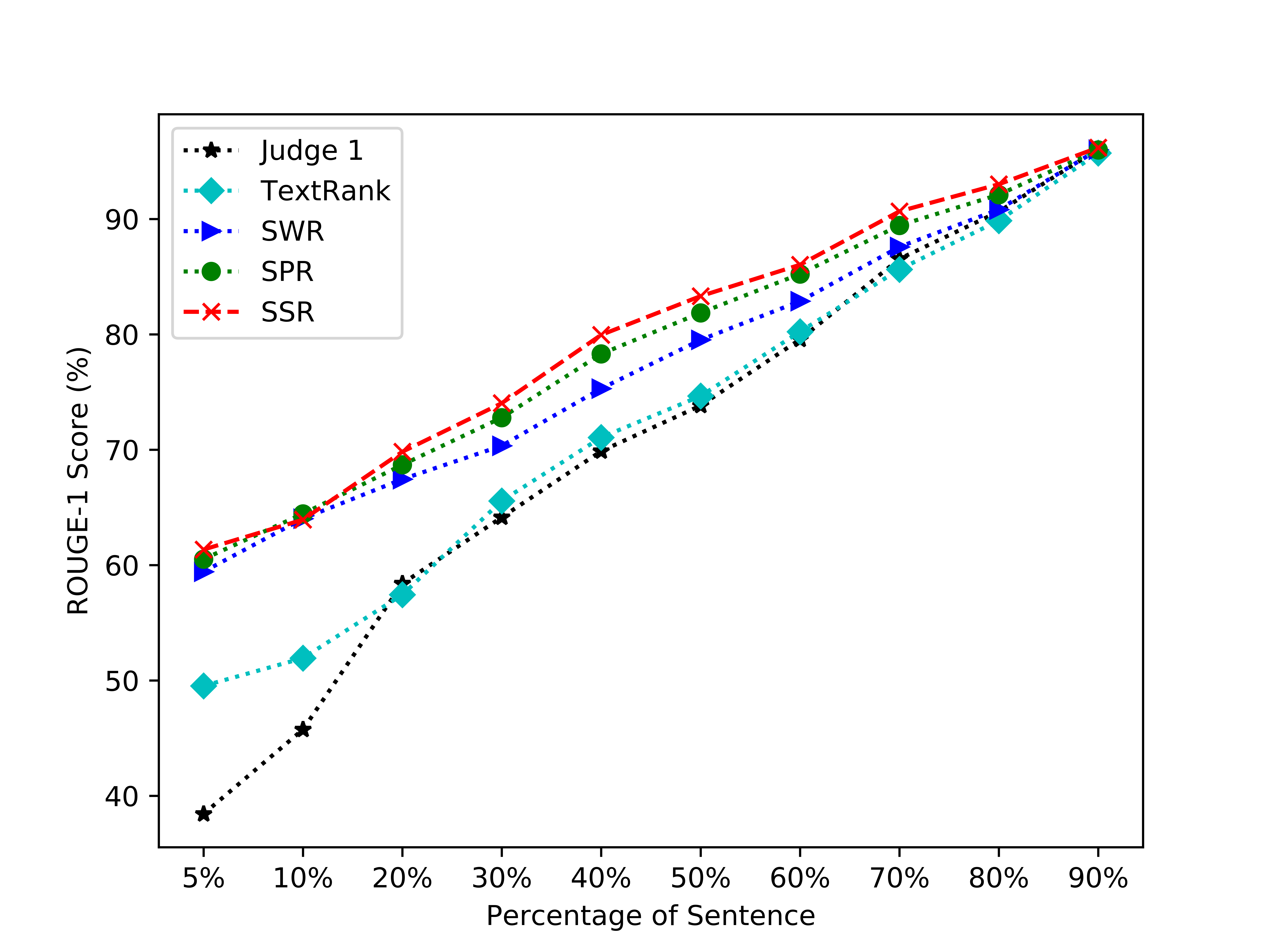
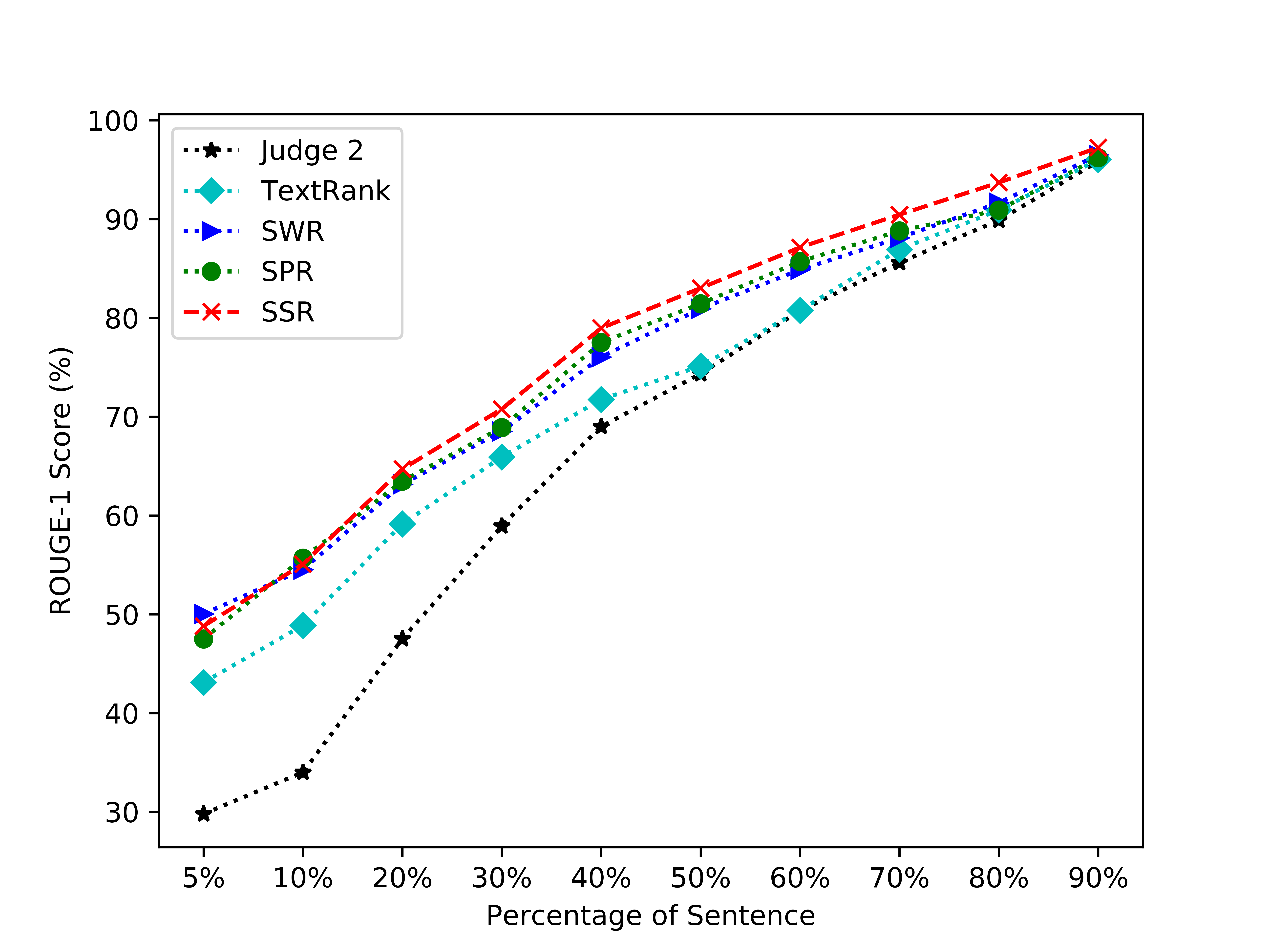
(a) Judge 1	(b) Judge 2
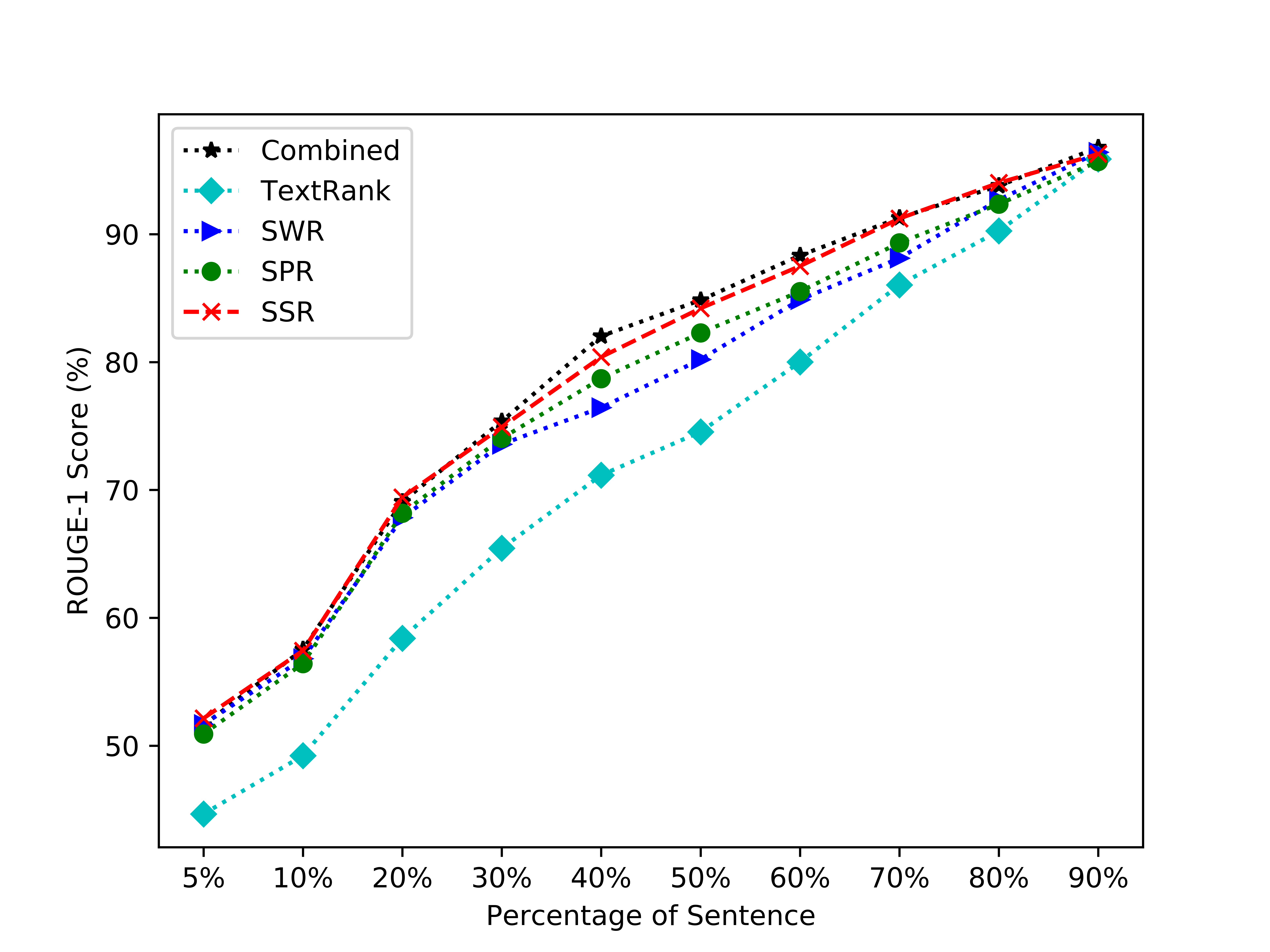
(a) Judge 3	(b) Combined ranking of all judges

Figure 2: ROUGE-1 (%) comparisons of individual judges and combined ranking with TextRank, SWR, SPR, and SSR over the SummBank benchmarks: (a) Judge 1 against Judges 2 and 3; (b) Judge 2 against Judges 1 and 3; (c) Judge 3 against Judges 1 and 3; (d) Combined ranking against all judges

The following results are evident:

1. Under all categories, SSR outperforms each judge by a significant margin and also outperforms SPR, which outperforms SWR, and SWR significantly outperforms TextRank.

2. SSR slightly outperforms the combined ranking of all judges under ROUGE-1, and is slightly below but very close to the combined ranking under ROUGE-2 and ROUGE-SU4, with the percentage differences being, respectively, 0.029%, 0.104%, and 0.109%. Moreover, SPR is slightly below SSR, SWR is slightly below SPR, and TextRank is substantially below SWR.

A full range of comparisons under ROUGE-1 with individual judges and the combined ranking of all judges are given at Fig. 2, where the percentage indicates that a portion of sentences are selected according to their ranks by the underlying methods. Thus, when 90% or more sentences are selected, all methods are comparable.

To demonstrate the robustness of an algorithm, it is customary to also compare ROUGE-2 and ROUGE-SU4 scores against the corresponding

Table 4: Full-range comparisons of SSR, SPR, SWR, and TextRank with individual judges and the combined ranking of all judges over the SummBank benchmarks, where shaded numbers in a group of comparisons for an individual judge are the highest scores under the corresponding measures, while in the group of comparisons for combined ranking, the shaded numbers are the highest and the second highest scores

references. An algorithm is robust if it compares consistently against the references under different ROUGE measures. Full-range comparisons under the ROUGE-2 and ROUGE-SU4 measures (see Table 4) show similar trends to those under ROUGE-1, indicating that SSR, SPR, and SWR are robust. Table 4 shows the comparison results from 10% top-ranked sentences to 90%, with an increment of 10% each time.

It follows from Table 4 that, under the ROUGE-1, ROUGE-2, and ROUGE-SU4 measures, comparison results similar to those on the 5% top-ranked sentences discussed on Table 3 hold true on the entire spectrum. More specifically,

1. SSR is better than SPR and is comparable with the combined ranking of all judges at all percentage levels with slightly smaller scores.

2. SPR is better than SWR and narrows the gap between SWR and the combined ranking.

3. SWR is significantly better than TextRank.

   1. SWR is substantially better than each individual judge’s ranking.

   2. SWR is compatible on top ranked sentences (up to 30%), but incurs a moderate gap on lower ranked sentences between 30% and 90%.

4. TextRank is substantially worse than the combined ranking of all judges. On the other hand, TextRank is better than individual judges on sentences of higher ranks but worse on sentences of lower ranks.

   1. Comparison with Judge 1: TextRank is better on top ranked sentences (up to 20%) and worse on the rest of the sentences.

   2. Comparison with Judge 2: TextRank is much better on top ranked sentences (up to 30%) and slightly better on the rest of the sentences.

   3. Comparison with Judge 3: TextRank is better or comparable on top ranked sentences (up to 30%), worse on lower ranked sentences from 30% to 70%, and comparable on the rest of the sentences.

TextRank is based only on co-occurrences of words for computing sentence scores, considering neither semantic information, nor subtopic diversity, nor structure of the underlying document. Incorporating these three features is expected to significantly improve the accuracy of sentence ranking, and the experiment results confirm that it is true. While incorporating semantics of words is better than without them, incorporating semantics of phrases and words is better than just using semantics of words, and adding semantics of sentences is even better.

It will be shown next how word semantics, article structure, Softplus function adjustment, and subtopic clustering each contribute to the improvement of sentence ranking.

8.7 Significance of each feature

It is interesting to understand how each of the features of semantic edges, Softplus function adjustment, ASB PageRank, and subtopic clustering actually contributes to the improvement of sentence rankings. To answer this question it suffices to evaluate the basic model SWR by removing a feature from it one at a time. Let SWR_NSE, SWR_NAS, SWR_NSC, and SWR_NSP denote, respectively, the variant of SWR without semantic edges, article-structure information, subtopic clustering, and Softplus adjustment.

Table 5 is the results obtained from evaluations over SummBank on selections of 10%, 40%, and 70% of sentences. TextRank is included as a baseline. The numbers in bold are the most severe drops, indicating that the corresponding features are the most critical.

Table 5: ROUGE (%) comparison with different features removed

Methods	R-1	R-2	R-SU4	R-1	R-2	R-SU4	R-1	R-2	R-SU4
	10%			40%			70%
SWR	56.82	48.18	47.03	76.48	71.74	70.39	88.21	86.17	85.19
SWR_NSE	55.02	46.08	45.15	71.98	66.76	65.42	85.94	83.18	81.83
SWR_NAS	51.74	40.87	40.13	73.52	68.26	67.12	87.82	84.95	84.12
SWR_NSC	56.36	47.34	46.44	75.68	70.35	69.03	87.54	84.49	83.54
SWR_NSP	56.77	48.12	46.97	76.39	71.59	70.25	88.14	86.04	85.07
TextRank	49.22	36.07	35.29	71.16	65.47	63.94	86.04	83.52	82.29

The following results are drawn:

1. With each of the features removed, the corresponding ROUGE scores drop, indicating that each feature has contributed to the improvement.

2. when the percentage of selecting sentences is smaller, removing article structure results in much larger drops, indicating that article structures are more significant on top-ranked sentences.

3. When the percentage becomes larger, semantic edges would become increasingly more critical.

4. While the Softplus function adjustment does improve ROUGE scores, it is not as significant as the other features.

5. Each SWR variant outperforms TextRank under all ROUGE measures, except that at the 70% level, when semantic edges are removed, SWR_NSE is lightly below TextRank.

Note that it is difficult to capture the underlying meanings of polysemous words using word-embedding representations, for one word-embedding representation cannot reflect different meanings. To train different word-embedding representations for a polysemous word so that each representation corresponds to only one meaning, it needs a corpus of documents containing the word only in one meaning. This is a formidable task because a document may contain multiple polysemous words, and each of these words may actually appear with one meaning here and a different meaning there in the same document. Even if multiple word-embedding representations could be trained for a polysemous word, it would still be challenging to determine which embedding representation should be used for a particular occurrence of the word. Using co-occurrences of words and phrases can help recoup the underlying meaning of a polysemous word lost in its word-embedding representation.

9 Conclusions and final remarks

SSR is an efficient and accurate scheme for ranking sentences of a given document. In particular, an implementation of SSR presented in this paper runs in quadratic time, and outperforms, on the SummBank benchmarks, each individual human judge’s ranking under standard ROUGE measures and compares well with the combined ranking of all judges. Moreover, extracting sentences of the highest ranks with an appropriate number of sentences as an extractive summary achieves the state-of-the-art results over the DUC-02 benchmarks under standard ROUGE measures.

SSR is an unsupervised scheme that does not rely on language-specific features or deep linguistic computations, and so it is readily adaptable across languages. What it needs is a reasonable corpus of digital documents available in the adapted language (such as Wikipedia dumps) for extracting phrases and training word and phrase embedding representations. However, the similarity threshold values presented in this paper for constructing a semantic word graph and a semantic phrase graph for a given document, while appropriate for the English language and not sensitive to a small change, may need to be adjusted for other languages. Better threshold values can be determined using a small amount of labeled data. When no labeled data is available, an expected number of synonyms may be used to determine appropriate thresholds [55].

It would be interesting to figure out how much weight should be given to the word-embedding similarity in a semantic-word graph and a semantic-phrase graph to better reflect the underlying meaning of a polysemous word. It would also be interesting to seek if there are more effective, unsupervised methods, incorporating nearby monosemous words in the context, to help bring out the underlying meaning of a polysemous word. The accuracy of the word-embedding-based WMD semantic measure of two sentences used in a semantic-sentence graph also suffers from polysemous words contained in them. A better way to handle polysemous words would be needed for improvement.

Not reported in this paper, location-score functions for sentences can be further improved to better reflect the structure of the underlying article in the following four categories: narration, argumentation, research, and news. Improved location-score functions have been implemented at http://dooyeed.com.

The following directions may be explored for further improvement of accuracy, in addition to what has been mentioned in the earlier sections:

1. Investigate other embedding methods such as ELMo [56], LEAR [57], Poincaré embeddings [58], hierarchical embedding [59], and spherical embedding [60].

2. Investigate unsupervised sentence representations such as skip-thought vectors [61] and BERT [62].

3. Fine-tune location scoring for better representing article structures.

4. Explore new approximation algorithm for the NP-hard multi-objective knapsack problem. For example, instead of using round-robin approximation that treats each cluster equally likely, a weighted round-robin strategy that treats each cluster according to the subtopic distribution in the given document may help improve accuracy.

Finally, readers should keep in mind that employing new methods, while possibly improving accuracy, may also degrade efficiency. Whether a trade-off is acceptable depends on the underlying applications.

References

- [1] Das D, Martins AF. A survey on automatic text summarization. Literature Survey for the Language and Statistics II Course at CMU. 2007;4(57):192–195.
- [2] Wang J, Zhang H, Zhang C, Yang W, Shao L, Wang J. An effective scheme for generating an overview report over a very large corpus of documents. In: Proceedings of the 19th ACM Symposium on Document Engineering (DocEng 2019); 2019. .
- [3] Neto JL, Santos AD, Kaestner CA, Alexandre N, Santos D, et al. Document clustering and text summarization. 2000;.
- [4] Mihalcea R, Tarau P. Textrank: Bringing order into text. In: Proceedings of the 2004 Conference on Empirical Methods in Natural Language Processing; 2004. .
- [5] Bhartiya D, Singh A. A Semantic Approach to Summarization. arXiv preprint arXiv:14061203. 2014;.
- [6] Bellare K, Sarma AD, Sarma AD, Loiwal N, Mehta V, Ramakrishnan G, et al. Generic text summarization using WordNet. In: Proceedings of Internationational Conference on Language Resources and Evaluation; 2004. .
- [7] Li W, Wu M, Lu Q, Xu W, Yuan C. Extractive summarization using inter-and intra-event relevance. In: Proceedings of the 21st International Conference on Computational Linguistics and the 44th annual meeting of the Association for Computational Linguistics. Association for Computational Linguistics; 2006. p. 369–376.
- [8] Nallapati R, Zhai F, Zhou B. SummaRuNNer: a recurrent neural network based sequence model for extractive summarization of documents. In: Proceedings of the 31st AAAI Conference on Artificial Intelligence; 2017. p. 3075–3081.
- [9] Radev D, et al.. SummBank 1.0 LDC2003T16. Web Download; 2003. Philadelphia: Linguistic Data Consortium.
- [10] Hu B, Chen Q, Zhu F. Lcsts: A large scale chinese short text summarization dataset. arXiv preprint arXiv:150605865. 2015;.
- [11] Mikolov T, Yih Wt, Zweig G. Linguistic regularities in continuous space word representations. In: Proceedings of the 2013 Conference of the North American Chapter of the Association for Computational Linguistics: Human Language Technologies; 2013. p. 746–751.
- [12] Kusner M, Sun Y, Kolkin N, Weinberger K. From word embeddings to document distances. In: Proceedings of the 32nd International Conference on Machine Learning; 2015. p. 957–966.
- [13] Shang J, Liu J, Jiang M, Ren X, Voss CR, Han J. Automated phrase mining from massive text corpora. IEEE Transactions on Knowledge and Data Engineering. 2018;30(10):1825–1837.
- [14] Dueck D. Affinity propagation: clustering data by passing messages. University of Toronto; 2009.
- [15] DUC. Document Understanding Conference; 2014. https://www-nlpir.nist.gov/projects/duc/intro.html.
- [16] Kupiec J, Pedersen J, Chen F. A trainable document summarizer. In: Proceedings of the 18th annual international ACM SIGIR conference on Research and development in information retrieval; 1995. p. 68–73.
- [17] Conroy JM, O’eary DP. Text summarization via hidden markov models. In: Proceedings of the 24th annual international ACM SIGIR Conference on Research and development in information retrieval; 2001. p. 406–407.
- [18] Cheng J, Lapata M. Neural summarization by extracting sentences and words. arXiv preprint arXiv:160307252. 2016;.
- [19] Narayan S, Papasarantopoulos N, Cohen SB, Lapata M. Neural extractive summarization with side information. arXiv preprint arXiv:170404530. 2017;.
- [20] Narayan S, Cohen SB, Lapata M. Ranking sentences for extractive summarization with reinforcement learning. arXiv preprint arXiv:180208636. 2018;.
- [21] Zhang Y, Er MJ, Pratama M. Extractive document summarization based on convolutional neural networks. In: Proceedings of the 42nd Annual Conference of the IEEE Industrial Electronics Society. IEEE; 2016. p. 918–922.
- [22] Erkan G, Radev DR. Lexrank: Graph-based lexical centrality as salience in text summarization. Journal of Artificial Intelligence Research. 2004;22:457–479.
- [23] Brin S, Page L. The anatomy of a large-scale hypertextual Web search engine. Computer Networks and ISDN Systems. 1998;30(1–7):107–117.
- [24] Wan X, Xiao J. Exploiting neighborhood knowledge for single document summarization and keyphrase extraction. ACM Transactions on Information Systems. 2010;28(2).
- [25] Wan X. Towards a unified approach to simultaneous single-document and multi-document summarizations. In: Proceedings of the 23rd International Conference on Computational Linguistics. Association for Computational Linguistics; 2010. p. 1137–1145.
- [26] Li L, Zhou K, Xue GR, Zha H, Yu Y. Enhancing diversity, coverage and balance for summarization through structure learning. In: Proceedings of the 18th international conference on World wide web; 2009. p. 71–80.
- [27] Parveen D, Strube M. Integrating importance, non-redundancy and coherence in graph-based extractive summarization. In: Proceedings of the 24th International Joint Conference on Artificial Intelligence; 2015. p. 1298–1304.
- [28] Parveen D, Mesgar M, Strube M. Generating coherent summaries of scientific articles using coherence patterns. In: Proceedings of the 2016 Conference on Empirical Methods in Natural Language Processing; 2016. p. 772–783.
- [29] Kleinberg JM. Authoritative sources in a hyperlinked environment. In: Proceedings of the 9th ACM-SIAM Symposium on Discrete Algorithms. ACM and SIAM; 1998. p. 668–677.
- [30] Isonuma M, Mori J, Sakata I. Unsupervised neural single-document summarization of reviews via learning latent discourse structure and its ranking. In: Proceedings of the 57th Annual Meeting of the Association for Computational Linguistics. ACL; 2019. p. 2142–2152.
- [31] Zhang H, Wang J. Semantic WordRank: generating finer single-document summarizations. In: Lecture Notes in Computer Sciences, Proceedings of the 19th International Conference on Intelligent Data Engineering and Automated Learning (IDEAL 2018). Springer; 2018. p. 398–409.
- [32] Po¨ttker H. News and its communicative quality: the inverted pyramid—when and why did it appear? Journalism Studies. 2003;4(4):501–511.
- [33] Florescu C, Caragea C. A position-biased PageRank algorithm for keyphrase extraction. In: Proceedings of the 31st AAAI Conference on Artifical Intelligence; 2017. p. 4923–4924.
- [34] Brin S, Page L. The anatomy of a large-scale hypertextual web search engine. Computer Networks and ISDN Systems. 1998;30(1-7):107–117.
- [35] Shao L, Zhang H, Jia M, Wang J. Efficient and effective single-document summarizations and a word-embedding measurement of quality. In: Proceedings of the 9th International Joint Conference on Knowledge Discovery, Knowledge Engineering and Knowledge Management - (Volume 1), Funchal, Madeira, Portugal, November 1-3, 2017.; 2017. p. 114–122.
- [36] Bloch F, Jackson MO, Tebaldi P. Centrality Measures in Networks; 2016.
- [37] Tinkham T. The effects of semantic and thematic clustering on the learning of second language vocabulary. Second Language Research. 1997;13(2):138–163.
- [38] Hearst MA. TextTiling: Segmenting text into multi-paragraph subtopic passages. Computational linguistics. 1997;23(1):33–64.
- [39] Von Luxburg U. A tutorial on spectral clustering. Statistics and Computing. 2007;17(4):395–416.
- [40] Besbes G, Zghal H. Personalized and context-aware retrieval based on fuzzy ontology profiling. Integrated Computer Aided Engineering. 2016 01;24.
- [41] Lehoucq R, Sorensen D. Implicitly restarted Lanczos method. In: Templates for the Solution of Algebraic Eigenvalue Problems: a Practical Guide (Zhaojun Bai et al eds.). SIAM;. .
- [42] Fränti P, Sieranoja S. How much can k-means be improved by using better initialization and repeats? Pattern Recognition. 2019;93:95–112.
- [43] Hartigan JA, Wong MA. Algorithm AS 136: A k-means clustering algorithm. Journal of the Royal Statistical Society Series C (Applied Statistics). 1979;28(1):100–108.
- [44] Kaufman L, Rousseeuw PJ. Finding groups in data: an introduction to cluster analysis. vol. 344. John Wiley & Sons; 2009.
- [45] Miettinen K. Nonlinear Multiobjective Optimization. Kluwer Academic Publishers; 1999.
- [46] Branke J, Deb K, Miettinen K, Slowiński R. Multiobjective Optimization: Interactive and Evolutionary Approaches. Springer; 2008.
- [47] Cheng J, Zhang G, Caraffini F, Neri F. Multicriteria adaptive differential evolution for global numerical optimization. Integrated Computer Aided Engineering. 2015 01;22:103–117.
- [48] Rostami S, Neri F. Covariance matrix adaptation Pareto archived evolution strategy with hypervolume-sorted adaptive grid algorithm. Integrated Computer-Aided Engineering. 2016;23(4):313–329.
- [49] Pan L, He C, Tian Y, Su Y, Zhang X. A region division based diversity maintaining approach for many-objective optimization. Integrated Computer-Aided Engineering. 2017;24(3):279–296.
- [50] Liu H, Wang Y, Liu L, Li X. A two phase hybrid algorithm with a new decomposition method for large scale optimization. Integrated Computer-Aided Engineering. 2018;25(4):349–367.
- [51] Yan X, He F, Zhang Y, Xie X. An optimizer ensemble algorithm and its application to image registration. Integrated Computer-Aided Engineering. 2019;26(4):311–327.
- [52] Bojanowski P, Grave E, Joulin A, Mikolov T. Enriching word vectors with subword information. arXiv preprint arXiv:160704606. 2016;.
- [53] Atasu K, Parnell T, Dünner C, Sifalakis M, Pozidis H, Vasileiadis V, et al. Linear-complexity relaxed word Mover’s distance with GPU acceleration. In: Proceedings of 2017 IEEE International Conference on Big Data. IEEE; 2017. p. 889–896.
- [54] Lin CY. ROUGE: a package for automatic evaluation of summaries. In: Proceedings of the Workshop on Text Summarization Branches Out, Post-Conference Workshop of ACL 2004; 2004. .
- [55] Rekabsaz N, Lupu M, Hanbury A. Exploration of a threshold for similarity based on uncertainty in word embedding. In: European Conference on Information Retrieval. Springer; 2017. p. 396–409.
- [56] Peters ME, Neumann M, Iyyer M, Gardner M, Clark C, Lee K, et al. Deep contextualized word representations. arXiv preprint arXiv:180205365. 2018;.
- [57] Vulić I, Mrkšić N. Specialising word vectors for lexical entailment. arXiv preprint arXiv:171006371. 2017;.
- [58] Nickel M, Kiela D. Poincaré embeddings for learning hierarchical representations. In: Proceedings of the 31 Annual Conference on Advances in Neural Information Processing Systems; 2017. p. 6338–6347.
- [59] Ai Q, Zhang Y, Bi K, Chen X, Croft WB. Learning a hierarchical embedding model for personalized product search. In: Proceedings of the 40th International ACM SIGIR Conference on Research and Development in Information Retrieval. ACM; 2017. p. 645–654.
- [60] Batmanghelich K, Saeedi A, Narasimhan K, Gershman S. Nonparametric spherical topic modeling with word embeddings. In: Proceedings of the 54th Annual Meeting of the Association for Computational Linguistics. vol. 2016. NIH Public Access; 2016. p. 537.
- [61] Kiros R, Zhu Y, Salakhutdinov RR, Zemel R, Urtasun R, Torralba A, et al. Skip-thought vectors. In: Proceedings of the 29th Annual Conference on Advances in Neural Information Processing Systems; 2015. p. 3294–3302.
- [62] Devlin J, Chang MW, Lee K, Toutanova K. Bert: Pre-training of deep bidirectional transformers for language understanding. arXiv preprint arXiv:181004805. 2018;.