Spectroscopic Studies of 30 Short-period Cataclysmic Variable Stars,
and Remarks on the Evolution and Population of Similar Objects

Abstract

We present spectroscopy and orbital periods $P_{\rm orb}$ for 30 apparently non-magnetic cataclysmic binaries with periods below $\sim 3$ hours, nearly all of which are dwarf novae, mostly of the SU Ursae Majoris subclass. We then turn to the evidence supporting the prediction that short-period dwarf novae evolve toward longer periods after passing through a minimum period – the ‘period bounce’ phenomenon. Plotting data from the literature reveals that for superhump period excess $\epsilon=(P_{\rm sh}-P_{\rm orb})/P_{\rm orb}$ below $\sim 0.015$, the period appears to increase with decreasing $\epsilon$, agreeing at least qualitatively with the predicted behavior. Next, motivated by the long ($\sim$ decadal) outburst intervals of the WZ Sagittae subclass of short-period dwarf novae, we ask whether there could be a sizable population of ‘lurkers’ – systems that resemble dwarf novae at minimum light, but which do not outburst over accessible timescales (or at all), and therefore do not draw attention to themselves. By examining the outburst history of the Sloan Digital Sky Survey sample of CVs, which were selected by color and not by outburst, we find that a large majority of the color-selected dwarf-nova-like objects have been observed to outburst, and conclude that ‘lurkers’, if they exist, are a relatively minor part of the CV population.

1 Introduction

Cataclysmic variable stars (CVs) are close binary systems consisting of a degenerate dwarf primary and a more extended star that transfers mass onto the degenerate component through Roche lobe overflow. Most CVs appear as dwarf novae, which undergo outbursts of 2-10 magnitudes from a quiescent state. The outburst interval varies widely, from nearly continuous to many years. The cause of the outburst is thought to be an accretion disk instability that occurs when material accumulating in the disk reaches a critical optical depth (Meyer & Meyer-Hofmeister, 1981; Smak, 1984).

The SU Ursae Majoris stars (Patterson, 1979; Vogt, 1980) are a subclass of dwarf novae that show superoutbursts. These are distinguished from normal outbursts by their higher amplitudes and longer duration. Within (typically) several days after the onset of a superoutburst, superhumps develop. Superhumps are photometric oscillations at a nearly constant period, $P_{\rm sh}$ that is almost always slightly longer than the orbital period $P_{\rm orb}$. Nearly all SU UMa stars have $P_{\rm orb}$ shortward of the $\sim 2$-3 hr ‘gap’ in the $P_{\rm orb}$ distribution. The generally accepted explanation for superhumps (see, e.g., Whitehurst, & King (1991)) begins with the fact that in these short-period systems, the mass ratio $q=M_{2}/M_{\rm WD}$ is low, which is a consequence of the condition that the secondary fills its Roche critical lobe (Faulkner et al., 1972; Patterson, 1984; Knigge, 2006). This makes the (mostly empty) Roche lobe around the white dwarf relatively large, making it possible for the outbursting disk to expand enough that the disk’s edge reaches a 3:1 resonance with the orbit. After the disk expands to the resonant radius, it becomes elongated and precesses slowly in the inertial frame. The tidal stresses raised by the secondary in the disk are greatest when the secondary aligns with the disk’s long axis. Because of the precession, the disk brightens at a frequency slightly lower than the orbital frequency, since each successive passage of the secondary through the disk’s long axis occurs a little later in orbital phase.

Some authors define a WZ Sagittae subclass of the SU UMa stars, which (1) undergo only superoutbursts, with no ‘normal’ ones, and (2) typically outburst at intervals of a decade or more. WZ Sge stars tend to have very short $P_{\rm orb}$s, typically near 75-85 min.

The fractional superhump period excess,

$$\epsilon={P_{\rm sh}-P_{\rm orb}\over P_{\rm orb}},$$ (1)

is thought to be related to the mass ratio $q$. This is physically plausible since the secondary’s gravity drives the disk precession. Patterson et al. (2005) used known mass ratios (derived largely from eclipse studies) to calibrate the relationship between $q$ and $\epsilon$. As noted earlier, the mass ratio of a CV is strongly correlated with $P_{\rm orb}$, because the secondaries of longer-period CVs must fill correspondingly larger Roche lobes. Consequently, the underlying $q(\epsilon)$ relation creates the observed relationship between $\epsilon$ and $P_{\rm orb}$. In non-eclipsing systems, $P_{\rm orb}$ can be difficult to establish; by contrast, superoutbursting stars are bright enough, and the superhumps distinct enough, that skilled amateur astronomers with small telescopes and CCD photometers routinely measure superhump periods. Assuming that $\epsilon$ is typical, one can infer $P_{\rm orb}$ from $P_{\rm sh}$ to within about one percent.

The mass ratio, for which $\epsilon$ serves as a proxy, is a key parameter in CV evolution. In nearly all CVs, $q<1$, and the mass transfer is stable in the sense that, when mass is lost from the secondary, its radius should decrease more quickly than the size of its Roche lobe, shutting off mass transfer. The evolution of CVs is therefore thought to be driven by the loss of orbital angular momentum, probably through magnetic braking of the co-rotating secondary at long periods, with gravitational radiation dominating at the shortest periods. There is one startling prediction – around $P_{\rm orb}\sim 70$ min, the secondary becomes degenerate and its radius begins to increase with decreasing mass. This leads to a gradual outspiral of the orbit following the period minimum. CVs in this stage are referred to as post-bounce CVs, though the reversal of the period evolution should be much more gradual than the phrase suggests. If post-bounce systems exist, they should be distinguished by very low mass ratios, and hence anomalously small $\epsilon$ for their $P_{\rm orb}$. Patterson (2011) presents a lucid and wide-ranging discussion of this phenomenon.

Dwarf nova outbursts are not the only channel through which CVs are discovered. Others are found from their X-ray emission (see Halpern & Thorstensen 2015 for a recent example), peculiar colors (typically ultraviolet excesses; see, e.g., the series of Sloan Digital Sky Survey (SDSS) CV papers ending with Szkody et al. 2011), or in spectral surveys (e.g., Aungwerojwit et al. 2006, Witham et al. 2007, 2008). Many of the objects found through channels other than outburst searches are ‘novalike variables’, a catchall class that has come to mean ‘CVs that are not dwarf novae’. Some appear to be in extended outburst states, as if their disks are in a stable high state; these include the UX UMa stars and the SW Sex stars. Many others have highly magnetized white dwarfs, and appear as AM Her stars (also called polars) or DQ Her stars (intermediate polars).

The space density of CVs constrains evolutionary and population-synthesis models. However, because of the large variety of discovery channels, it is difficult to estimate the completeness of the known sample of CVs. The majority of CVs were found because they are outbursting dwarf novae. However, the outburst interval introduces a ‘wild card’ into the completeness estimate; the outburst intervals of WZ Sge stars can exceed a decade, and there is no obvious reason why they could not be much longer. The WZ Sge stars all have orbital periods near the $\sim$75 minute minimum; if there is a substantial population of “lurkers” – dwarf novae with extremely long recurrence intervals – we expect them to be found among the shortest orbital periods, which we focus on here. We will return to this question in Section 4.2.

Here we present spectroscopic periods for 30 CVs that prove to have periods shortward of, or near, the 2-3 hr gap. One motivation is to refine and strengthen the $\epsilon$-$P_{\rm orb}$ relation. Many CVs in outburst are quickly found to be superhumping, and $P_{\rm sh}$ is used to estimate $P_{\rm orb}$ (see e.g. Gänsicke et al. 2009); this practice depends on the $\epsilon$-$P_{\rm orb}$ relation, but and obviously cannot be used to improve that relation without an independent determination of $P_{\rm orb}$. An independent $P_{\rm orb}$ is also needed to reveal post-bounce systems, if they exist. Leaving aside the $\epsilon$-$P_{\rm orb}$ relation, orbital periods of non-outbursting systems are needed to see if they be “lurking” WZ Sge stars. Finally, the good signal-to-noise resulting from the long cumulative exposures required for spectroscopic periods sometimes reveals spectral anomalies.

2 Observations and Reductions

All the observations reported are from the MDM Observatory on Kitt Peak, Arizona, and nearly all are spectra.

Most are from the ‘modspec’ spectrograph, mounted either on the Hiltner 2.4m telescope or the McGraw-Hill 1.3m telescope. For nearly all modspec observations, the detector was a SITe 2048² CCD giving 2 Å per 24 $\mu$m pixel. and a useful range from 4310 to 7500 Å, with severe vignetting toward the ends of the range. A few observations were taken with a 1024² SITe chip with the same pixel spacing, set up to cover from 4600 to 6800 Å. For wavelength calibration we used spectra of Hg, Ne, and Xe comparison lamps taken in twilight to establish the shape of the pixel-wavelength relation, and then adjusted for instrument flexure during the night using the strong $\lambda$5577 night-sky line. We also observed flux standard stars, but our average fluxes suffer from estimated uncertainties of at least 20 per cent due to cloudy intervals and uncalibrated losses at the slit, which had a projected width of $1.^{\prime\prime}1$ at the 2.4 m and $2.^{\prime\prime}0$ at the 1.3 m. Spectra taken with the modspec often show unphysical variations in the continuum shapes, which we do not understand, but these do tend to average out over large numbers of exposures.

Our most recent observations are from the Ohio State Multi-Object Spectrometer (OSMOS; Martini et al. 2011), mounted on the 2.4m and configured to give a spectrum from 3975 to 6870 Å, with a dispersion of 0.7 Å pixel^-1 and a FWHM resolution of $\sim 4$ Å. The wavelength calibration of the OSMOS is not as stable as that of the modspec, so we maintained an accurate wavelength scale by taking comparison lamps before and/or after our object spectra, and using these to both shift and ‘stretch’ calibrations derived from lamp spectra taken at the zenith. Target acquisition with OSMOS requires at least one direct image. We took those (generally 20 s exposures) with a Sloan $g$ filter, and used the PAN-STARRS PSF magnitudes of many stars in the field to derive the magnitude zero point and hence the target’s $g$ magnitude just before we took our spectra. As with the modspec data, we derived a spectrophotometric calibation from standard stars; the flux-calibrated continua with OSMOS were usually more physically plausible than with modspec.

The short-period CVs studied here undergo ten or more orbital cycles per day. Our observations – from a single site, at night – are necessarily taken on a roughly 24-hour cycle. This creates aliasing in the period determination – if the sampling were strictly periodic, the number of cycles occurring during the day would be unconstrained. To ameliorate this, we break the 24-hour sampling periodicity by observing at large hour angles, where atmospheric dispersion (Filippenko, 1982) can be problematic. By default, the spectrograph slit is oriented north-south, which is on the parallactic angle at the meridian. For observations away from the meridian, we compute $|\tan Z\sin x|$, where $Z$ is the zenith distance and $x$ is the angle between the position angle of the slit and the parallactic angle; any dispersion effect will be proportional to this cross-slit refraction factor. For our spectral coverage, slit width, and typical seeing, we reckon that dispersion losses should be acceptable when the cross-slit factor is substantially less than 1. The observation planning software JSkyCalc (written by the author) includes a tool for computing this factor as a function of time; when it shows the cross-slit refraction factor growing too large, we rotate the instrument to an appropriate angle, except for at the 1.3 m, where rotation is less convenient and the wider projected slit ameliorates the problem.

We reduced the data mostly with python-language scripts calling IRAF tasks through Pyraf. For extracting 1-dimensional spectra from the two-dimensional images, we mostly used a C-language implementation of the algorithm described by Horne (1986), while for the most recent OSMOS data we used a python implementation of Horne’s algorithm. The H$\alpha$ emission line invariably gave the most useful radial velocities; to measure these, we used a convolution algorithm described by Schneider & Young (1980). For broader lines, we used dual-gaussian convolution functions that emphasized the steep sides of the line profile, and for narrow lines we used the derivative of a gaussian optimized for the line’s width. To estimate velocity uncertainties, we took the uncertainty in each pixel (computed from the gain, read noise, and background), and propagated them forward to compute the error in location of the convolution zero-crossing. This is a lower limit, since it ignores systematic offsets caused by line profile variations and other effects.

To search the velocity time series for periods, we used a ‘residual-gram’ algorithm that fits least-squares sinusoids at each of a dense grid of fixed frequencies; the figure of merit is $1/\chi^{2}$, where $\chi^{2}$ is the mean of the squared residuals scaled to their estimated errors. Well-sampled data from multiple nights show alias frequencies separated from the best frequency by 1 cycle d^-1 because of the cycle count issue discussed earlier. To assess the reliability of the alias choice, we used the Monte Carlo test described by Thorstensen & Freed (1985).

Once a period was determined, we fit the time series with sinusoids

$$v(t)=\gamma+K\sin[2\pi(t-T_{0})/P],$$ (2)

where the epoch $T_{0}$ was chosen to be near the mean epoch of the observations (to minimize the correlation between $T_{0}$ and $P$), but within one cycle of an observation. To estimate parameter uncertainties, we used the prescription of Cash (1979), which in practice amounts to perturbing each parameter until $\chi^{2}$ is roughly $1+1/N$ of its minimum value, where $N$ is the number of data points. The Monte Carlo tests (Thorstensen & Freed, 1985) generate parameter uncertainties as a byproduct; these agree well with those calculated from the other procedure.

In many cases we have observations from two or more widely separated observing runs, which are fit well by large numbers of possible precise periods corresponding to integer numbers of cycles between runs. If rough periods could be estimated from the isolated data of more than one run, we estimated the period by fitting each run’s velocities individually and taking a weighted average.

3 Results

Below, we discuss the stars individually in order of right ascension; Table 1 gives names and accurate coordinates. Table 2 lists radial velocities derived from the individual exposures, and serves as a record of when the stars were observed. Figures 1 – 3 and 5 – 9 show mean spectra, periodograms, and folded velocity data for each star. Table 3 gives parameters of sinusoidal fits to the velocities.

Table 1: List of Objects

Name	$\alpha_{\rm ICRS}$	$\delta_{\rm ICRS}$	$G$	$1/\pi_{\rm DR2}$
	[h:m:s]	[d:m:s]		[pc]
FL Psc	00:25:11.038	+12:17:11.81	17.53	153.5(+3.3,$-$3.1)
1RXS J012750.5+380830 J0127+3808	01:27:50.595	+38:08:11.83	17.24	366(+34,$-29$)
CRTS CSS121120 J020633+205707	02:06:33.463	+20:57:07.19	18.25	490(+60,$-50$)
WY Tri	02:25:00.476	+32:59:55.55	17.63	490(+35,$-$30)
BB Ari	02:44:57.797	+27:31:09.14	18.45	353(+25,$-$22)
SDSS J032015.29+441059.2	03:20:15.287	+44:10:59.20	18.87	473(+62,$-$49)
MASTER OT J034045.31+471632.2	03:40:45.292	+47:16:31.56	18.71	680(+182,$-$119)
V1024 Per	04:02:39.048	+42:50:45.82	17.06	251.0(+4.7,$-$4.5)
V1389 Tau	04:06:59.822	+00:52:43.81	18.40	561(+71,$-$57)
Gaia 19emm	04:34:36.596	+18:02:44.79	17.40	439(+32,$-28$)
V1208 Tau	04:59:44.043	+19:26:22.72	18.62	555(+137,$-$92)
ASAS-SN 15pq	05:21:15.867	+25:13:32.15	16.94	$254\pm 8$
1RXS J05573+685	05:57:18.463	+68:32:26.78	18.29	678(+82,$-$66)
SDSS J0751+10	07:51:16.993	+10:00:16.26	18.43	480(+50,$-$40)
SBS 0755+600	07:59:26.372	+59:53:51.06	18.31	435(+43,$-$36)
TT Boo	14:57:44.746	+40:43:40.50	18.95	679(+105,$-$80)
QZ Lib	15:36:16.018	$-$08:39:08.60	18.88	187(+12,$-$11)
CSS170517:155156+1453334	15:51:55.625	+14:53:33.08	18.43	1400(+1200,$-$450)
SDSS J155720.75+180720.2	15:57:20.764	+18:07:20.19	18.76	847(+258,$-$166)
IX Dra	18:12:31.451	+67:04:45.61	17.40	790(+39,$-$36)
ASAS-SN 13at	18:21:22.503	+61:48:55.16	19.40	870(+280,$-$170)
KIC 11390659	18:58:30.923	+49:14:32.65	16.37	$259\pm 3$
RX J1946.2-0444	19:46:16.357	$-$04:44:56.86	17.44	365(+14,$-$13)
V1316 Cyg	20:12:13.648	+42:45:50.95	18.07	661(+65,$-$55)
ASAS-SN 14ds	20:44:55.871	$-$11:51:52.55	16.82	393(+15,$-$14)
V444 Peg	21:37:01.839	+07:14:45.69	18.64	405(+43,$-$35)
ASAS-SN 14cl	21:54:57.695	+26:41:12.95	18.19	261(+14,$-$12)
V368 Peg	22:58:43.478	+11:09:11.92	19.06	537(+138,$-$91)
IPHAS 2305	23:05:38.375	+65:21:58.63	18.79	617(+103,$-$77)
NSV14652	23:38:48.669	+28:19:54.82	18.38	627(+102,$-$77)

Note. — Positions, mean $G$ magnitudes, and distances from the GAIA Data Release 2 (DR2; Gaia Collaboration et al. 2016a, b). Positions are referred to the ICRS (essentially the reference frame for J2000), and the catalog epoch (for proper motion corrections) is 2015. The distances and their error bars are the inverse of the DR2 parallax $\pi_{\rm DR2}$, and do not include any corrections for possible systematic errors.

3.1 FL Psc (= ASAS 002511+1217.2)

This object was object was discovered in superoutburst by the All Sky Automated Survey (ASAS; Pojmanski 1997) on 2004 Sep. 11 UT, at $V=10.49$ (Price et al., 2004). Templeton et al. (2006) present a study of the superoutburst, and find superhumps with a period of 0.05687(1) day during the interval from 5 to 18 days after the discovery. Kato et al. (2009), find a significantly larger value, $0.057093(12)$, from an analysis of a more complete data set and by restricting their analysis to the ‘plateau’ stage of the outburst. After this, the source faded to magnitude $\sim 15$ for a few days before undergoing a single brief ‘echo’ outburst around day 25; during this fainter interval a photometric period near 0.05666(3) day was detected, which Templeton et al. (2006) suggested was probably not orbital because it was too close to the superhump period. A brief series of spectra during the decline showed strong, double-peaked Balmer lines, modulated in velocity at about 82 minutes; the shortness of the time series precluded a precise determination of $P_{\rm orb}$.

FL Psc has apparently remained quiescent since its 2004 outburst, though an outburst could have been missed due to its low ecliptic latitude. Its CRTS DR2 light curve covers from 2004 to 2014, and shows it near $\sim 17.3$, with variations of typically a few tenths of a magnitude.

Most of our spectra were taken 2004 Nov 18 – 21 UT, starting 68 days after the initial detection, after the source had returned to quiesence (Templeton et al., 2006). The mean spectrum (Fig. 1) shows a blue continuum with double-peaked Balmer emission. At the suggestion of T. Kato, we obtained more spectra in 2018 November with a 6-day time span to improve the precision of $P_{\rm orb}$ to 0.05604(9) d. The number of cycles that elapsed in the 14-year interval between observing runs is unknown. Kato et al. (2009) found a candidate $P_{\rm orb}=0.056540(3)$ d from photometry taken late in the superoutburst. This is significantly longer than the spectroscopic period we find here, 0.05604(9) d; our spectroscopic period gives a significantly larger superhump period excess than the photometric period.

3.2 1RXS J012750.5+380830

Hu et al. (1998) discovered this CV (hereafter referred to as RX J0127+38) as the optical counterpart of a ROSAT X-ray source; it is listed in the Downes et al. (2001) catalog. The CRTS2 light curve includes 291 points between 2005 and 2014, and shows irregular variations by a few tenths of a magnitude around a typical magnitude of 16.9, but no outbursts. An outburst to $V=14.8$ is reported in vsnet-alert 19909 .

Our mean spectrum (Fig. 1) has good signal-to-noise and shows relatively weak features such as the iron feature near $\lambda 5169$ and He II $\lambda 4686$. The Balmer lines are strong and just barely double-peaked.

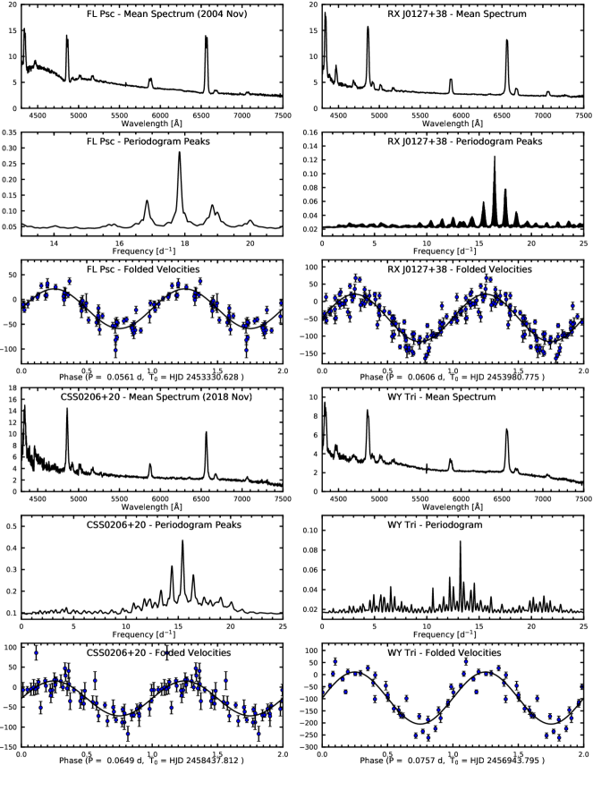
Figure 1: Caption on next page.

Figure 1: Average spectra, periodograms, and folded velocity curves for FL Psc, RX J0127, CSS 0206+20, and WY Tri. The vertical scales, unlabeled to save space, are (1) for the spectra, $f_{\lambda}$ in units of $10^{-16}$ erg s^-1 cm^-2 Å^-1; (2) for the periodograms, $1/\chi^{2}$ (dimensionless); and (3) for the radial velocity curves, barycentric radial velocity in km s^-1. In cases where velocities are from more than one observing run, the periodogram is labeled with the word “peaks”, because the curve shown is formed by joining local maxima in the full periodogram with straight lines. This suppresses fine-scale ringing due to the unknown number of cycle counts between runs. The folded velocity curves all show the same data plotted through two cycles for continuity, and the best-fit sinusoid (see Table 3) is also plotted. The velocities shown are H$\alpha$ emission velocities.

3.3 CRTS CSS121120 J020633+205707

This object, hereafter referred to as CSS 0206+20, is one of many dwarf novae discovered in the Catalina Real Time Transient Survey (CRTS; Drake et al. 2009; Breedt et al. 2014; Drake et al. 2014b). A possible superoutburst was noted by Kato in vsnet-alert 20577, but superhumps have apparently not been detected. (See Fig. 1.)

3.4 WY Tri

WY Tri was discovered by Meinunger (1986). Liu & Hu (2000) obtained a spectrum showing the broad emission lines typical of a CV at minimum light, and Vanmunster (2001) found superhumps with a period of 0.07847(2) d, establishing the object as an SU UMa star. (See Fig. 1.)

3.5 BB Ari

BB Ari was discovered by Ross (1927). Its CRTS2 light curve has 268 detections between 2005 and 2014, and shows variation mostly between 17.8 and 18.8 mag in quiescence, with only a single eruption to 14.3 in late 2012. ASAS-SN (Shappee et al., 2014) detected the object at 13.9 in 2013 August – a brightening missed by CRTS2 – and a superoutburst followed. Kato et al. (2014b) analyzed data from this; they give superhump periods $P_{1}=0.072544(97)$ and $P_{2}=0.072135(46)$ day.

Our spectra (Fig. 2) were taken on four observing runs. The entire velocity time series is fit best by $P=0.0702472(1)$ d, but this level of precision assumes that the cycle count between observing runs is unambiguous. Monte Carlo tests suggest that the cycle-count choice can be made with $\sim 90$ per cent confidence. The next two, less-likely candidate periods are 0.0701099 and 0.0699820 d; the first of these differs from the best period by one cycle per 36 days.

3.6 SDSSJ032015.29+441059.2

This object (SDSS J0320+44 herafter), was identified as a CV by Wils et al. (2010), who searched for dwarf novae by data mining and cross-comparing several catalogs. It has $g=18.77$ in the SDSS, and they found outbursts to 14.7 mag on two occasions in archival catalogs. Its sky position is not covered in the CRTS2. Several outbursts have been reported on vsnet-alert since its discovery, but superhumps have apparently not been seen. (See Fig. 2.)

3.7 MASTER OTJ034045.31+471632.2

This object (Fig. 2) was discovered by the MASTER survey at 15.6 mag on 2013 December 26 (Denisenko et al., 2013b); we will refer to it as OT J0340+47. The authors note a previous outburst on a 1993 Sky Survey plate, and that the object’s location is not covered by CRTS. Photometric monitoring by Hardy et al. (2017) did not find an eclipse. A superoutburst occurred in early 2019, and Vanmunster reported superhumps with an amplitude of 0.21 mag and a period $P_{\rm sh}=0.0803(6)$ d (vsnet-alert 22925). Our radial velocities, from 2015 October and 2018 November, could not disambiguate candidate frequencies near 13.0 and 14.0 cycle d^-1. The Vanmunster superhump period breaks the ambiguity in favor of $1/P_{\rm orb}=13.0$ cycle d^-1.

3.8 V1024 Per = NSV1436

Kato et al. (2015) give background information on this object (Fig. 2), which was known as NSV 1436 before it was named V1024 Per. They analyzed data from a 2014 September outburst and derived superhump periods $P_{1}=0.072843(14)$ and $P_{2}=0.072403(43)$ d. The object has a companion about 3 arcsec to its south, which is not known to be associated except along the line of sight. It lies outside the CRTS2 coverage area.

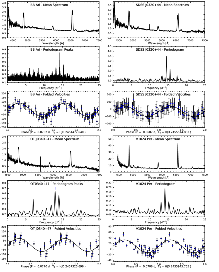
Figure 2: Similar to Fig. 1, but for BB Ari, SDSS J0320+44, OT J0340+47, and V1024 Per. The odd continuum shape for OT J0340+47 is likely to be an artifact. In the periodogram for that object, the tick mark in the periodigram shows the frequency selected by the superhump period.

3.9 V1389 Tau = OT J040659.8+005244

This object (Fig. 3) was first reported by Yamaoka et al. (2008a). Kato et al. (2009) analyzed data from its 2008 superoutburst and found a nearly constant superhump period of 0.07992(2) day; they suggested the source had been caught relatively late in the outburst, leading to a nearly constant period.

We have only 24 spectra, 16 from an observing run in 2009 October and the rest from 2010 November. The combined H$\alpha$ radial velocities define $P_{\rm orb}=0.0780(2)$ d. The number of cycles that elapsed between the runs is unknown, so we estimate the uncertainty in $P_{\rm orb}$ from fits to the individual observing runs. Our velocities do not independently establish the daily cycle count, but our best period is slightly shorter than $P_{\rm sh}$, as expected, so the alias choice is secure.

3.10 Gaia 19emm

The Gaia Alerts Index notes a brightening of this object by $\sim$ 1.5 mag on 2019 Oct. 6, and lists it as a candidate CV. The object lies 6.3 arcsec from the Einstein X-ray source 2E 0431.7+1756, and 13 arcsec from RX J0434.5+1802, and may be the optical counterpart.

The Gaia light curve shows multiple detections from 2015 onward, between G = 17 and 18, with one brightening in 2019 October that triggered the alert, while CRTS DR2 has it mostly between $V$ = 16.5 and 17.5, with a single brightening to $V$ = 15.8 on 2005 Sept. 28. Spectra obtained on the McGraw-Hill 1.3 m in 2019 Oct. 30 and 31, only a few weeks after discovery, showed the broad Balmer and He I emission typical of a dwarf nova at minimum light, at a signal-to-noise inadequate for a radial velocity study. Better and more extensive data obtained in 2020 January with the 2.4 m and OSMOS yielded an unambiguous radial velocity period of $123.55\pm 0.09$ min. The spectrum (Fig. 3) shows the strong, broad emission lines typical of dwarf novae at minimum light; the FWHM of H$\alpha$ is 1600 km s^-1 and its EW is 88 Å. The spectrum and orbital period are both typical for dwarf nova, but the outbursts so far recorded are rather weak.

3.11 V1208 Tau = Tau3

Motch et al. (1996) discovered this CV as the optical counterpart of a ROSAT X-ray source. It was listed in the Downes et al. (2001) catalog with the temporarily designation “Tau3”.

The CRTS2 light curve shows it typically near 18th magnitude, but with substantial scatter, going fainter than 19th on occasion, and a few points near 21st. There are at least nine outbursts, to 14.9 mag near maximum brightness. Kato et al. (2009) gives superhump periods $P_{1}=$ 0.070501(32) and 0.070537(27) day for two different outbursts; Kato et al. (2013) find $P_{2}=0.070481(66)$ day for a third, and suggest that all three determinations are actually for Stage C superhumps. Combining these yields $P_{\rm sh}=101.5(3)$ min.

The mean spectrum (Fig. 3) shows single-peaked emission lines on a flat continuum. The radial velocities do not constrain the daily cycle count independently, but the well-determined superhump period selects our best-fitting radial velocity period, which is 98.1(2) min.

3.12 ASAS-SN 15pq

This was discovered by ASAS-SN on 2015 Sept. 12, and reached $V\sim 16.3$. The CRTS DR2 has observations at 64 epochs that vary from 18.0 to 19.0, with one excursion to 17.5, so observations so far establish a rather modest outburst amplitude of $\sim 3$ mag. We have velocities from five observing runs. The first four yielded two possible periods 115.5(3) or 108.9(3) min. The 2020 January data resolved the ambiguity in favor of the longer period, giving 115.2(3) min for the 2020 January data alone. Superoutbursts and superhumps have apparently not been reported.

The sinusoidal fit parameters in Table 3 and the periodogram in Fig. 3 are derived from the 2020 January data. The phase-folded velocity plot (also Fig. 3) also includes points from the other runs.

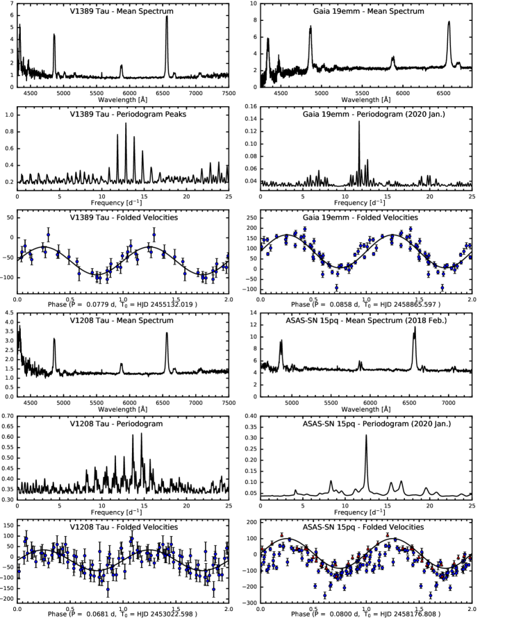
Figure 3: Similar to Fig. 1, but for V1389 Tau, Gaia 19emm, V1208 Tau, and ASAS-SN 15 pq. In the folded velocity plot for ASAS-SN 15pg, the red triangles are the 2020 January data used to compute the periodogram, and the amplitude and zero point of the solid curve are fitted to those points, which are systematically high compared to the velocities from the other observing runs.

3.13 Var Cam 06 = 1RXS J055722.9+683219

Uemura & Arai (2006) reported the first known outburst of this object, and attribute the discovery to W. Kloehr; they also found apparent superhumps. The object lies 25 arcsec from a ROSAT X-ray source (1RXS J055722.9+683219) and is the likely optical counterpart. We will refer to it as 1RXS J0557+685. Uemura et al. (2010) gave details of this superoutburst and another some 480 d later; they found $P_{\rm sh}$ to be relatively short at 0.05324(2) day, or 76.66 min, indicating that the orbital period is also short. The 480-d interval between superoubursts suggest that they are relatively frequent compared to many short-period SU UMa stars. Uemura et al. (2010) reviewed data on dwarf novae with similarly short periods, and suggested that this object belongs to a natural grouping that combines very short period, relatively short outburst recurrence times, and supherhump period excesses that are larger than expected for the orbital period. On this basis they suggested that $P_{\rm orb}$ should be 0.05209(1) d, or roughly 75.01(2) min.

The spectrum (Fig. 5) is somewhat unusual. The He I lines are atypically strong; He I $\lambda$5876 in particular is a bit less than half the flux of H$\alpha$. Although the signal-to-noise degrades badly toward the blue, He II $\lambda$4686, is also clearly detected. There is no evidence for a secondary star spectrum, but the object is relatively faint, with a synthesized $V$ magnitude near 19.3, limiting the signal-to-noise ratio to $\sim 20$ per 2 Å pixel in the best-exposed parts of the spectrum. The spectrum is reminiscent of, but less extreme than, that of the dwarf nova SBS 1108+574 (Carter et al., 2013), which has $P_{\rm orb}=55.3$ min, and a ratio of He I $\lambda 5876$ to H$\alpha$ of 0.81. In addition, both that object and the present one show weak emission centered on 6356 Å, which Carter et al. (2013) attribute to a blend of Si II $\lambda\lambda$ 6347 and 6371. SBS 1108+574 shows broad absorption wings in the higher Balmer lines that are attributed to the white dwarf in the system, but these are not evident here.

The measured orbital period, 75.34(38) min, agrees within the mutual uncertainty with the period predicted by Uemura et al. (2010).

3.14 SDSSJ075117.00+100016.2

Wils et al. (2010) identified this object (hereafter SDSS J0751+10) as a CV. Spectra from five observing runs in 2010 and 2011 did not reveal an unambiguous period, but a more concerted effort in 2020 Jan. showed the period to be 85.28(7) min, which also fits the earlier velocities acceptably well. As with ASAS-SN 15pq, the parameters in Table 3 and the periodogram (Fig. 5) are from the 2020 January data alone, but the folded velocity plot includes all the data.

3.15 SBSS 0755+600

Stepanian et al. (1999) took spectra of a sample of objects from the Second Byurkan Survey and classified this as a CV. It appears in outburst on the POSS-I images (obtained through the Digital Sky Survey at STScI), which were taken 1954 January 5. The outburst images show the CV slightly brighter than a field star near $\alpha=7^{\rm h}59^{\rm m}24^{\rm s}.00,\delta=+59^{\circ}52^{\prime}31^{\prime\prime}.0$, about 80 arcsec south and somewhat west of the CV; the APASS catalog lists $V=15.7$ for this star. The finding chart in the Downes et al. (2001) catalog is incorrect – the CV is slightly northwest of the object they mark. Fig. 4 shows the correct star. The CRTS light curve has 120 points, but no outbursts; the magnitude reaches 17.39 and sometimes fades to fainter than 19th, reaching 20.51 on a single occasion. (See Fig. 5.)

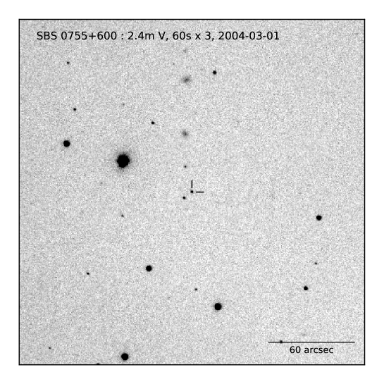
Figure 4: Finding chart for SBSS 0755+60, from the median of three 60 s $V$-band exposures taken with the MDM 2.4m telescope on 2004 March 1 UT. North is at the top and east is to the left, and the scale is indicated.

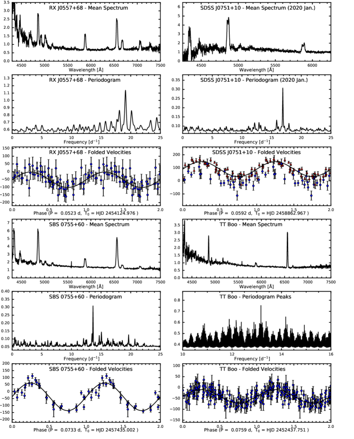
Figure 5: Similar to Fig. 1, but for 1 RXS J05573+865, SDSS J0751+10, SBSS 0755+600, and TT Boo. The downturn at the blue end of the spectrum of SDSS J0751+10 is unlikely to be real. For the same star, the 2020 January velocities are shown with red triangles, and again appear to be systematically high compared to the velocities from other runs. A 3-point boxcar smoothing has been applied to the (oversampled) spectrum.

3.16 TT Boo

This is among the longer-known objects considered here (Chernova, 1951). It is an SU UMa star with numerous well-observed superoutbursts (Kato et al., 2009, 2012, 2013) giving $P_{\rm sh1}$ near 0.0780 d, or 12.82 c d^-1. The CRTS2 has 228 points covering about 9 years, and shows the star mostly near 19th magnitude, with three outbursts, one of which reaches 13.34.

We have 127 velocities taken on many runs over a span of 5552 days. The daily cycle count is not definitive, but strongly favors a value near 13.168 c d^-1, as expected from the superhump period. We nearly have a nearly unambiguous run-to-run cycle count, the only remaining ambiguity being a splitting at one cycle per 5000 days. The small period uncertainty quoted in Table 3 reflects this. (See Fig. 5.)

3.17 QZ Lib = ASAS J153616-0839.1

This object was discovered in outburst in 2004 by ASAS. It showed superhumps at $P_{1}=0.064602(24)$ day (Kato et al., 2009). Apparently no outbursts have been observed since then, suggesting a WZ Sge classification. Our mean spectrum (Fig. 6) shows strong, relatively narrow Balmer emission lines and apparent broad absorption wings at H$\beta$, apparently from an underlying white dwarf contribution.

Our radial velocities do not span enough hour angle range to independently determine a period. However, only one of our daily cycle-count aliases – the second-best one – is consistent with the well-determined $P_{\rm sh}$, so we adopt this, and find $P_{\rm orb}=0.06411(7)$ d. Taking $P_{1}$ from Kato et al. (2009) as $P_{\rm sh}$ gives $\epsilon=0.0071\pm 0.0013$, suggesting a very low mass ratio.

After our data were collected, Pala et al. (2018) published a detailed study of QZ Lib. They independently determined $P_{\rm orb}=0.06436(20)$, consistent with our determination but with a slightly larger formal uncertainty. They calculate a mass ratio $q=M_{2}/M_{\rm WD}=0.040(9)$, find $T_{\rm WD}=10500\pm 1500$K, and conclude that QZ Lib is likely to have passed through its period minimum, making it a period “bouncer”.

3.18 CSS170517:155156+1453334

This object (hereafter CSS 1551+14) was discovered at magnitude 15.64 on 2017 May 17. The CRTS DR2 has 302 epochs over a span of 3000 days, and shows variation between 17.2 and 19.0 at minimum light, and two outbursts to around 15.5, that escaped notice at the time.

Our velocities (Fig. 6) are from 2017 June, not long after the discovery. The observations are a bit sparse; the velocities strongly favor a period of 100.3(3) min, but aliases are not entirely excluded.

3.19 SDSS J155720.75+180720.2

Szkody et al. (2009) discovered this object (hereafter SDSS 1557+18) in the SDSS; it lies 8 arcseconds from the ROSAT X-ray source 1RXS J155720.3+180715 and is the likely optical counterpart. Szkody et al. (2009) derived a preliminary period near 2 hours from a short run of radial velocity data. In its CRTS2 light curve it appears consistently near 18th magnitude, but at 14.8 mag in 2007 June 13 and 16.2 on 2008 June 9. A further outburst was reported by Jeremy Shears on 2015 July 30 (vsnet-alert 18914), and another was found by CRTS in 2016 March (vsnet-alert 19602); during this last outburst J. Hambsch established $P_{\rm sh}$ = 0.08538(6) d. (See Fig. 6.)

3.20 IX Dra

This dwarf nova outbursts frequently; Olech et al. (2004) give 3.1(1) and 54(1) d for the mean cycle and supercycle lengths, respectively. Olech et al. (2004) obtained time-series photometry during a 2003 September superoutbust and established $P_{\rm sh}=0.066968(17)$ day, or 96.43(2) min. Intriguingly, their photometry showed a second periodicity at 0.06646(6) day, or 95.70(8) min, only 0.76 per cent shorter than the superhump. They pointed out that identifying this second period with $P_{\rm orb}$ implies a very small mass ratio. If confirmed, this would make the system an excellent candidate for a post-bounce CV (see the Introduction).

The very short outburst cycle made it difficult to obtain a usable velocity time series; on multiple visits over the years, we found it either in full outburst with absorption lines, or well above minimum light with relatively weak emission. In 2014 June we finally found the star in a fairly low state with tractable emission lines (Fig. 6). We obtained 29 radial velocities on three successive nights, after which the source returned to outburst. From the velocities we find $P_{\rm orb}=0.06480(16)$ d, or 93.31(23) min, 3.3 per cent shorter than $P_{\rm sh}$. This is consistent with the $\epsilon$ - $P_{\rm orb}$ relation, so the system is (perhaps disappointingly) apparently not post-bounce.

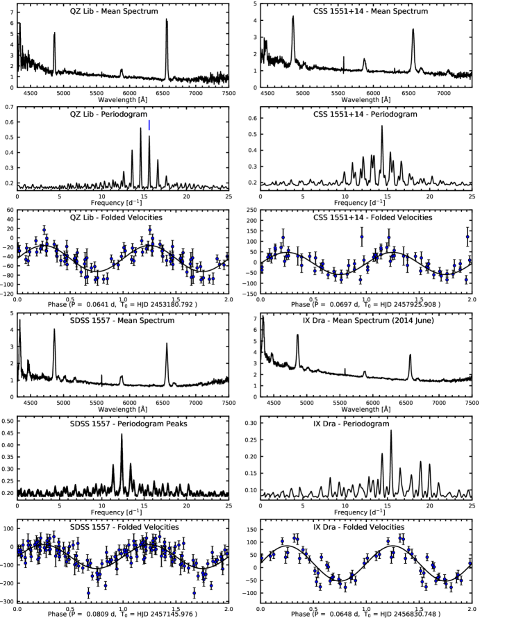
Figure 6: Similar to Fig. 1, but for QZ Lib, CSS 1551, SDSSS 1757, and IX Dra. In the periodogram for QZ Lib, the tick mark indicates the adopted orbital period (based on $P_{\rm sh}$). In SDSS 1557+18, the upturn in the continuum longward of H$\alpha$ is probably an artifact.

3.21 ASAS-SN 13at = MASTER OT J182122.59+614854

This object was discovered independently by the ASAS-SN and MASTER surveys (Stanek et al., 2013; Denisenko et al., 2013a). Our observations are from 2013 Sept., 2014 June, and 2018 June, and define $P_{\rm orb}=0.0790(2)$ d without ambiguity in the daily cycle count, although the number of cycles elapsed between observing runs is unknown. (See Fig. 7)

3.22 KIC 11390659

Howell et al. (2013) obtained spectra of this Kepler object showing strong double-peaked emission lines typical of a dwarf nova at minimum light. A short radial-velocity time series indicated a period of 106-109 min. We observed the source on three successive nights in 2018 May with the McGraw-Hill 1.3m telescope, and found an unambiguous period of 110.80 $\pm 0.17$ min, apparently consistent with that found by Howell et al. (2013) (see Fig. 7). The Kepler light curve showed only irregular variations, but the ASAS-SN survey found an outburst on 2013 July 3. Photometry during that outburst did not reveal any superhumps (Pavol A. Dubovsky, Tamas Tordai and Tonny Vanmunster, vsnet-alert 18729). A subsequent outburst was observed in 2017 May by Tadashi Kojima (vsnet-alert 20982), again without any superhump detection.

3.23 RX J1946.2-0444

This object was discovered by Motch et al. (1998) in the Rosat Galactic Plane Survey, and catalogued by Downes et al. (2001). Its position is not covered in CRTS DR2, and apparently nothing about its variability has appeared in the literature.

We observed this on three observing runs in the 2007. Although outbursts have not been observed, the mean spectrum (Fig. 7) appears entirely typical of dwarf novae at minimum light. Our observations were sufficient to establish an unambiguous cycle count for the data set, allowing us to establish a relatively precise $P_{\rm orb}=107.46(1)$ min.

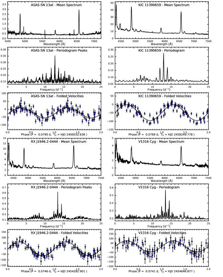
Figure 7: Similar to Fig. 1, but for ASAS-SN 13at, KIC 11390659, RX J1946.7-0444, and V1316 Cyg. The velocities do not determine the period of ASAS-SN 14cl unambiguously; the adopted period, chosen for consistency with the superhump period, is indicated in the periodogram.

3.24 V1316 Cyg

Romano (1967) discovered this variable star (first designated GR 141) and later classified it as a dwarf nova (Romano, 1969). Boyd et al. (2008) detected superhumps at 0.07685(3) d, which transitioned to 0.07654(2) d later in the outburst. Fig. 7 summarizes our data.

3.25 ASAS-SN 14ds

ASAS-SN detected an outburst from this source 2014 July 08 (Holoien et al., 2014), designated it ASAS-SN 14ds, and identified it with the X-ray source 1RXS J204455.9$-$115151. Denisenko (vsnet-alert 17478) drew attention to at least one previous outburst, and noted that the source varies by about 1 mag in quiescence. However, Hardy et al. (2017) obtained a $\sim 5$ hr light curve during outburst and found no eclipse. We obtained an exploratory spectrum with the Hiltner telescope and OSMOS in 2016 August, which appeared typical of a dwarf nova, and much more extensive modspec data 2018 August and September with the McGraw-Hill 1.3m and Hiltner 2.4m respectively that unambiguously indicated a period near 2.53 hr, squarely in the period gap (Fig. 8). The weighted average of the periods from separate fits to the August and September data is 0.1058(3) d. The two runs are close enough together that there are relatively few viable choices of cycle count over the inter-run gap; the resulting periods can summarized as

$$P_{\rm orb}={25.553\pm 0.007\ {\rm d}\over N},$$ (3)

where $N=242\pm 2$ is an integer.

3.26 V444 Peg = OT J213701.8+071456

This variable star was discovered on 2008 Nov. 6 by Yamaoka et al. (2008b). The 441 points in its CRTS2 light curve show it mostly fluctuating from 18th to 19th magnitude, with an outburst to 12.8 mag in 2012 September. there are also three points taken 2008 Nov. 21 near 16.6 mag, apparently near the end of the discovery outburst. Kato et al. (2009) gives $P_{1}=0.099451$ for the 2008 outburst (with no error estimated), and $P_{1}=0.097645(52)$ for the 2012 outburst.

The spectrum (Fig. 8) is unusual in that it shows a contribution from an M-dwarf secondary star; the signal-to-noise ratio does not permit an accurate classification of the secondary, but we estimate it to be M3 $\pm$ 1.5 subclasses from comparison with library spectra.

We find $P_{\rm orb}$ = 2.222(4) hr, at the lower edge of the period gap; the superhump period excess $\epsilon$ is then 0.073 using the value from the 2008 outburst, and 0.054 for the shorter $P_{\rm sh}$ in the 2012 outburst.

3.27 ASAS-SN 14cl

Stanek et al. (2014) announced the discovery of this transient, which reached $V=10.66$. Kato et al. (2015) give details of the outburst, and find superhump periods $P_{1}=0.060008(13)$ and $P_{2}=0.059738(14)$ d. The object was caught early enough that so-called ‘early superhumps’ – a photometric modulation that is apparently at the orbital period – were detected, yielding an estimated $P_{\rm orb}=0.05838$ d.

Our spectrum (Fig. 8) shows a relatively steep blue continuum and deep, broad $H\beta$ absorption flanking the emission line, both of which indicate a strong contribution from the white dwarf photosphere. The $H\alpha$ emission line had a low velocity amplitude, and we cannot independently determine an unambiguous $P_{\rm orb}$. However, one or our candidate periods, 0.05859(4) d, is apparently consistent with the early-superhump period, for which no uncertainty is quoted.

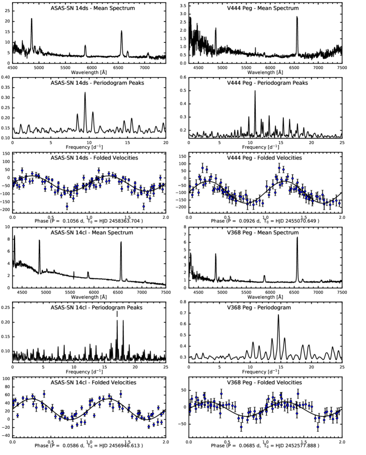
Figure 8: Similar to Fig. 1, but for ASAS-SN 14ds, V444 Peg, ASAS-SN 14cl, and V368 Peg.

3.28 V368 Peg = Antipin V63

Antipin (1999) discovered this star on archival plates, which showed 7 outbursts reaching as bright as 13.3 mag. Kato et al. (2009) and Kato et al. (2010) describe the superhump behavior in several different outbursts and found superhump periods near 0.07039 d. We find the amplitude of the H$\alpha$ emission velocity modulation to be quite low ($K=22\pm 5$ km s^-1), but were still able to determine $P_{\rm orb}=0.0685(3)$ d from data taken mostly on two successive nights in 2002 October (Fig. 8).

3.29 IPHAS 2305

This source was originally discovered as an H$\alpha$ emission source by the INT/WFC Photometric H$\alpha$ Survey (IPHAS), described by Witham et al. (2008). It is a possible optical counterpart of the ROSAT X-ray source 1RXS J230538.2+652155. A superoutburst in 2015 was analyzed by Kato et al. (2016), who found $P_{\rm sh}=0.0727$ d. We cannot independently find an unambiguous period from our radial velocities, which date from three nights in 2008 September, but the period that fits our data best – 0.0702(3) d – is nicely consistent with the superhump period, and we are confident that it represents $P_{\rm orb}$. It is marked in the periodogram (Fig. 9)

3.30 NSV14652 = CRTS J233848.7+281955

Kato et al. (2009) found $P_{\rm sh}=0.081513(16)$ d for a 2004 outburst of this SU UMa star, which SIMBAD lists by its CRTS designation given above. The Catalina Sky Survey detected an outburst on 2009 June 27. The CRTS DR2 light curve shows it mostly around 18th magnitude, with only a few outbursts, the brightest reaching 15th. Szkody et al. (2014) published a spectrum of the source in decline, showing Balmer emission lines. Our spectra (Fig. 9) appear similar.

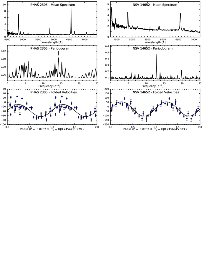
Figure 9: Similar to Fig. 1, but for IPHAS 2305 and NSV14652. The period adopted for IPHAS 2305, based on the superhump period, is indicated in the periodogram.

4 Discussion

Dwarf novae in this period range often show superoutbursts and superhumps. We measure $P_{\rm orb}$ independently of $P_{\rm sh}$ here, so we can compute empirical values of the superhump period excess $\epsilon$ for those stars that also have $P_{\rm sh}$.

4.1 The $\epsilon$-$P_{\rm orb}$ relation.

The superhump period excess $\epsilon=(P_{\rm sh}-P_{\rm orb})/P_{\rm orb}$ should be a good proxy for the mass ratio $q=M_{2}/M_{\rm WD}$; Patterson et al. (2005) calibrates this relationship empirically and approximates it as

$$\epsilon=0.18q+0.29q^{2},$$ (4)

which we adopt here.

Short-period CVs are thought to evolve to shorter periods until they reach a period minimum, after which they should evolve toward longer periods. On the $\epsilon$-$P_{\rm orb}$ diagram, one expects the ‘post-bounce’ systems to be objects with $P_{\rm orb}$ somewhat longer than the minimum period, and with $\epsilon$ (and hence $q$) smaller than expected, indicating a very low-mass secondary. Patterson (2011) lists 22 candidate post-bouncers, based on a variety of criteria. Since then, more have been proposed (e.g. Kimura et al. 2018; Nakata et al. 2014; McAllister et al. 2017; Pala et al. 2018).

In a remarkable series of papers (Kato et al., 2009, 2010, 2012, 2013, 2014a, 2014b, 2015, 2016, 2017, 2020), T. Kato and collaborators present extraordinarily extensive time series photometry of outbursting SU UMa stars. The papers also tabulate orbital periods, where known. The shorter-period objects in the sample, which tend to be seldom-outbursting WZ Sge stars, often show so-called early superhumps, which appear early in the outburst before the development of normal superhumps. These appear to be reliable indicators of the orbital period itself. Therefore, many of the shorter-period objects included in these papers have reasonably reliable $P_{\rm orb}$ from photometry alone; others have spectroscopic periods.

Fig. 10 shows the mass ratios $q$ inferred from the superhump period excesses $\epsilon$ (using, specifically, the average ‘Stage A’ superhump period, or $P_{1}$ in their notation) plotted against $P_{\rm orb}$. The curve shown is a polynomial for $P_{\rm orb}$ as a function of $q$, constructed by fitting the points from the Kato papers, rejecting points that missed the curve by more than 0.005 d ($\sim 7$ min), and iterating twice, in order to represent the apparent ‘ridgeline’ of the distribution. Its analytic form is

$$P_{\rm orb}=0.07276688-0.49012845\,q+3.89878883\,q^{2}-5.65565187\,q^{3},$$ (5)

where $P_{\rm orb}$ is in days, and the range of validity is as shown in Fig. 10. The curve reaches a minimum $P_{\rm orb}$ near 80 min, with $q\sim 0.075$, but individual systems reach significantly shorter periods. Fig. 11 is a magnified version of the turnaround region. Objects in the shaded region are evidently strong period-bounce candidates; Table 4 gives more detail on these objects.

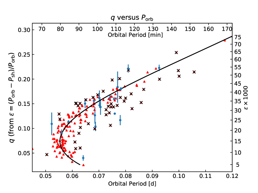
Figure 10: Mass ratios $q$ inferred from superhump period excesses, plotted against $P_{\rm orb}$. Small red triangles are from the series of papers by Kato et al.; blue dots with error bars are from the present work. The black curve is an iterative fit to the red points (see text). Points that were excluded by the iterative fit are marked with a black x-cross. The scale on the right axis gives the superhump period excesses corresponding to $q$.

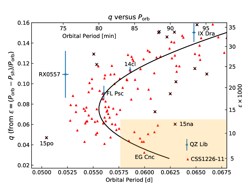
Figure 11: Magnified view of the turnaround portion of Fig. 10, with selected stars labeled. Names are abbreviated where necessary; 14cl, 15po, and 15na are from the ASAS-SN survey. The shaded portion shows strong bounce candidates.

The new orbital periods presented here contribute relatively little to this analysis. The most notable are QZ Lib, for which the uncertainties are reduced, and RX J0557+68, which has a short period and yet a fairly large $q$, though with substantial uncertainty. Uemura et al. (2010) noted the unusual nature of this object already (see Section 3.13). The newly-determined period of IX Dra is nicely consistent with the upper (pre-bounce) part of the evolutionary trajectory (Section 3.20).

4.2 Do all ‘dwarf novae’ undergo outbursts?

As noted in the Introduction, there are several discovery channels for CVs. Most CVs were historically discovered as dwarf novae in outburst, and this has remained the case, especially as the cadence and depth of all-sky surveys has dramatically improved. However, one object discussed here, RX J1946.2$-$0444, is not known to outburst, yet appears otherwise similar to the rest of the sample. Since short-period CVs tend to have low luminosities, they are relatively easy to overlook, which leads to the the question as to how many more non-outbursting objects remain undiscovered.

One way to attack this question compares the rate of new discoveries versus re-discoveries in a survey such as CRTS. From an analysis of discovery rate versus time, Breedt et al. (2014) suggest that the Catalina surveys had found most of the high-accretion-rate dwarf novae within their footprint and magnitude limits, but point out that low-accretion rate systems would still remain undiscovered. ASAS-SN is still discovering new dwarf novae, in part because it covers low Galactic latitudes that CRTS did not.

It is possible that these surveys could still be missing a population of systems that physically resemble dwarf novae at minimum light, but undergo outbursts on extremely long time scales (or possibly never). There is no obvious reason why such objects – which we will call lurkers – could not exist. Lurkers would necessarily have low mass transfer rates $\dot{M}$; if low enough, this could stretch the outburst interval to be arbitrarily long. Alternatively, some residual form of disk viscosity might be sufficient to maintain a steady state, again at sufficiently low $\dot{M}$.

To search for lurkers, we examined the sample of 284 CVs from SDSS, published in a series of annual papers by Szkody and others (Szkody et al., 2002, 2003, 2004, 2005, 2006, 2007, 2009, 2011). Importantly, these were not selected because of their variability, but rather by color and confirmed with follow-up spectroscopy,

To begin, we examined the SDSS spectra and selected those that appeared consistent with dwarf novae at minimum light. The classification criteria were (a) emission lines with relatively high equivalent width; (b) continua that did not slope up too steeply into the blue, unless white-dwarf absorption wings were visible around H$\beta$; (c) relatively broad emission lines; and (d) weak or absent He II emission. These criteria largely eliminate novalike variables, so-called ‘polars’ or AM Herculis stars, and systems for which the CV classification is questionable. This left 179 of the original 284 objects.

We divided our candidate dwarf nova spectra into three non-overlapping types. Objects with apparent late-type secondary contributions – which usually have orbital periods above $\sim 5$ hr – were classified as DN-2. Objects showing a white dwarf contribution – which must have low disk luminosities, and often have orbital periods below 3 hours – were designated DN-W. All others were simply DN.

Thirty-seven of the sample were rediscoveries of known outbursting dwarf novae. Eliminating these left 142 objects.

Our task was to find how many of these 142 have been found to outburst. This called for a complicated search, because individual outbursts are seldom written up as papers. We proceeded as follows.

As noted earlier, the archived vsnet-alert emails are a rich source of information on these stars, especially announcements of outbursts. To make these more accessible we scanned the email subject lines with a regular expression-based program that found variable star names, coordinate-based names, and names derived from, e.g., the ASAS-SN survey, and used the results to match the subject lines to a master list of CVs. We then checked the 142 remaining candidates for vsnet-alert messages, and found outburst notices for 81 of them, leaving 61 candidates remaining. The texts of the vsnet messages most often credited the Catalina surveys for the outburst trigger.

We next downloaded the CRTS-DR2 light curves for the remaining 61 candidates, and examined them for outbursts of greater than $\sim 1$ magnitude. This test was intentionally not stringent, because we were trying to isolate true non-outbursters. This yielded outbursts, or candidate outbursts, for another 26 objects from the sample. Four more were found outbursting in the Palomar Transient factory database, hosted at the NASA/IPAC Infrared Science Archive. We then turned to the DASCH interface (Digital Access to a Sky Century @ Harvard) which revealed outbursts of three more. We examined the entries in the American Association of Variable Star Observers (AAVSO) VSX database of variable stars, which eliminated one, and finally examined light curves for the locations from the ASAS-SN archive hosted at Ohio State, eliminating a single object. Finally, we examined the PAN-STARRS light curves and found no outbursts, which is not surprising given the relatively sparse time sampling.

After this, 22 objects remained. They are listed in Table 5, and broken down by type in Table 6. We draw the following conclusions.

First, the number of non-outbursting objects is remarkably small, and not compatible with a large population of lurkers. While some of the events we called ‘outbursts’ may have been questionable, it is also possible that some outbursts were missed. If we take the fraction of lurker candidates to known outbursters – 22/179, or about 12 per cent – to be representative of the CV population as a whole, it is likely that only 10 or 20 per cent of the DN-like objects within a few hundred parsecs outburst so infrequently as to remain undiscovered. Pala et al. (2019) reach broadly similar conclusions using different methods.

It should be noted that this limit applies only to objects that appear similar to quiescent dwarf novae, that is, that have $\dot{M}$ high enough to generate the broad emission lines that are the signature of a DN near minimum. Mass transfer might turn off for an extended period, as in the disrupted magnetic braking scenario invoked to explain the period gap. Also, the SDSS CV sample was selected by their blue colors; very old and slow-accreting systems might have white dwarfs that were too red to be included.

Table 5 also demonstrates a strong over-representation of systems with significant white-dwarf contributions in their spectra (DN-W systems) among the lurker candidates. These appear to be WZ Sge stars, which often have outburst intervals of a decade or more. It would not be surprising if all of DN-W systems in Table 5 were to outburst within the next couple of decades, but it remains possible that their outburst intervals could stretch still longer.

5 Acknowledgments

The National Science Foundation supported portions of this work through grants AST-0307413, AST-0708810, and AST-1008217.

We thank Taichi Kato for useful discussions, and for his tireless efforts compiling reliable superhump parameters, and we are grateful to the operators of the vsnet-alert system at Kyoto University. This work made extensive use of the online archive of the vsnet-alert messages, which retain their value long after the outbursts are over, and we are especially grateful to those who maintain it. We also thank Elmé Breedt for communicating the periods of two of the SDSS non-outbursters, and Tom Maccarone for pointing out that SDSS might have missed some CVs harboring cooler white dwarfs.

This research made use of the Digital Access to a Sky Century @ Harvard (DASCH), AAVSO, and Catalina Real-time Transient Survey databases. We acknowledge ESA Gaia, DPAC and the Photometric Science Alerts Team (http://gsaweb.ast.cam.ac.uk/alerts). This research made use of the NASA/IPAC Infrared Science Archive, which is funded by NASA and operated by the California Institute of Technology. The DASCH project at Harvard is grateful for partial support from NSF grants AST-0407380, AST-0909073, and AST-1313370.

Facilities: Hiltner, McGraw-Hill

FL Psc (catalog ) CRTS CSS121120 J020633+205707 (catalog ) WY Tri (catalog ) BB Ari (catalog ) SDSSJ032015.29+441059.2 (catalog ) MASTER OT J034045.31+471632.2 (catalog ) V1024 Per (catalog ) V1389 Tau (catalog ) 2E 0431.7+1756 (catalog ) V1208 Tau (catalog ) (catalog ASAS-SN 15pq) NAME Var Cam 06 (catalog ) SDSSJ075117.00+100016.2 (catalog ) SBSS 0755+600 (catalog ) TT Boo (catalog ) QZ Lib (catalog ) (catalog CSS170517:155156+145333) 1RXS J155720.3+180715 (catalog ) IX Dra (catalog ) ASASSN -13at (catalog ) V368 Peg (catalog ) 2MASS J18583091+4914326 (catalog ) RX J1946.2-0444 (catalog ) V1316 Cyg (catalog ) 1RXS J204455.9-115151 (catalog ) V444 Peg (catalog ) ASASSN -14cl (catalog ) V368 Peg (catalog ) 1RXS J230538.2+652155 (catalog ) CRTS J233848.7+281955 (catalog )

Table 2: Radial Velocities

Star	Time	$v_{\rm emn}$	$\sigma$
		[km s-1]	[km s-1]
FL Psc	53327.7397	$-$7	19
FL Psc	53327.7607	$-$62	7
FL Psc	53327.7708	$-$9	8
FL Psc	53327.7783	8	9
FL Psc	53328.5730	9	6

Note. — Table 2 is published in its entirety in the electronic edition of The Astronomical Journal, A portion is shown here for guidance regarding its form and content.

Table 3: Fits to Radial Velocities

Data set	$T_{0}$	$P$	$K$	$\gamma$	$N$	$\sigma$
		(d)	(km s-1)	(km s-1)		(km s-1)
FL Psc	53329.6182(10)	0.05604(9)	36(4)	$-17(3)$	36	13
1RXS J0127+3808	53980.7751(10)	0.06071(5)	69(7)	$-48(5)$	95	23
CSS 0206+20	58437.8125(16)	0.06489(18)	44(6)	$-28(5)$	53	18
WY Tri	56943.7952(17)	0.07569(7)	108(15)	$-97(11)$	32	40
BB Ari	54477.6396(12)	0.07024722(11)	79(9)	$9(6)$	62	29
SDSS J0320+44	55514.883(2)	0.06870(12)	72(14)	$-28(10)$	58	32
OT J0340+47	57320.696(3)	0.0770(4)	72(14)	$3(10)$	22	35
V1024 Per	55945.755(3)	0.0706(3)	23(6)	$10(4)$	41	14
V1389 Tau	55132.0190(18)	0.0780(2)	35(5)	$-58(4)$	24	13
Gaia 19emm	58865.5972(15)	0.08580(6)	81(10)	$87(7)$	46	31
V1208 Tau	53022.598(4)	0.06813(15)	50(17)	$-15(12)$	57	39
ASAS-SN 15pq	58867.6052(12)	0.0800(2)	92(10)	$8(6)$	20	23
1RXS J05573+685	54124.976(4)	0.0523(3)	50(23)	$-52(16)$	56	37
SDSS J0751+10	58865.6883(11)	0.05922(5)	58(7)	$90(5)$	45	22
SBSS 0755+600	57435.0023(16)	0.07334(7)	99(14)	$-37(10)$	30	33
TT Boo	52437.751(3)	0.07593962(7)	31(7)	$-40(5)$	127	21
QZ Lib	53180.7919(15)	0.06411(7)	28(4)	$-44(3)$	48	14
CSS 1551+14	57925.908(2)	0.06966(16)	53(12)	$-6(8)$	35	28
SDSS J1557+18	57145.976(2)	0.0810(2)	66(12)	$-55(9)$	75	39
IX Dra	56830.7477(20)	0.06480(16)	69(13)	$17(9)$	29	32
ASAS-SN 13at	57558.943(2)	0.0792(2)	33(6)	$-22(4)$	63	19
KIC 11390659	58249.7782(15)	0.07694(12)	47(6)	$-48(4)$	57	18
RX J1946.2-0444	54282.9008(13)	0.074624(6)	64(6)	$-1(5)$	62	22
V1316 Cyg	54646.877(3)	0.07412(13)	60(14)	$17(10)$	53	33
ASAS-SN 14ds	58363.704(3)	0.1058(3)	48(8)	$-35(5)$	55	25
V444 Peg	55070.649(3)	0.09260(18)	76(15)	$-96(10)$	47	34
ASAS-SN 14cl	56946.613(2)	0.05859(4)	26(5)	$25(4)$	36	13
V368 Peg	52577.888(3)	0.0685(3)	22(5)	$-5(4)$	45	13
IPHAS 2305	54711.979(4)	0.0702(3)	27(8)	$-37(6)$	37	20
NSV14652	56945.6030(14)	0.07824(8)	81(11)	$-24(7)$	26	25

Note. — Parameters of least-squares sinusoid fits to the radial velocities, of the form $v(t)=\gamma+K\sin(2\pi(t-T_{0})/P$.

Table 4: Candidate Period Bouncers

Name	$\alpha$	$\delta$	$\epsilon$	$q$	$P_{\rm orb}$	$P_{\rm orb}$
Ref.	[h:m:s]	[d:′:′′]			[d]	[min]
OT J111218-353837	11:12:17.40	$-$35:38:29.0	0.0085	0.0439	0.05847	84.2	1
EZ Lyn	08:04:34.20	+51:03:49.2	0.0103	0.0526	0.05901	85.0	1,3
PNV 17144255-2943481	17:14:42.60	$-$29:43:45.0	0.0090	0.0464	0.05956	85.8	7
MASTER 211258.65+242145.4	21:12:58.65	+24:21:45.4	0.0083	0.0431	0.05973	86.0	5
ASASSN-14cv	17:43:48.58	+52:03:46.8	0.0083	0.0430	0.05992	86.3	7
EG Cnc	08:43:04.04	+27:51:49.9	0.0061	0.0323	0.05997	86.4	1
ASASSN-16js	00:51:19.07	$-$65:57:16.9	0.0098	0.0506	0.06034	86.9	9
ASASSN-17fn	10:35:28.34	+54:19:07.5	0.0102	0.0524	0.06096	87.8	10
OT J220559.40-341434.9	22:05:59.40	$-$34:14:34.9	0.0116	0.0590	0.06129	88.3	9
ASASSN-15na	19:19:08.84	$-$49:45:41.0	0.0119	0.0603	0.06297	90.7	8
QZ Lib	15:36:16.02	$-$08:39:08.6	0.0188	0.0401	0.06411	92.3	T
CSS160414:122625-113303	12:26:25.43	$-$11:33:03.3	0.0048	0.0258	0.06420	92.4	9

Table 5: SDSS CVs Without Known Outbursts

Object	Ref.	Type	$P_{\rm orb}$	ref.	$g$	$G$	$\pi$	$\pi$ error	PM
SDSS			[min]		[mag.]	[mas]	[mas]	[mas]	[mas yr-1]
SDSS J003941.06+005427.5	4	DN-W	91	1	20.57	20.89	$-$1.3322	1.9534	21.35
SDSS J004335.14$-$003729.8	3	DN-W	82	2	19.84	19.88	2.9876	0.5716	29.45
SDSS J023003.79+260440.3	7	DN-2	$\cdots$	$\cdots$	19.91	19.05	1.6944	0.3488	6.80
SDSS J080534.49+072029.1	6	DN-2	330	3	18.52	17.90	0.5133	0.1708	6.04
SDSS J083754.64+564506.7	6	DN	$\cdots$	$\cdots$	18.97	$\cdots$	$\cdots$	$\cdots$	$\cdots$
SDSS J085623.00+310834.1	4	DN-W	$\cdots$	$\cdots$	19.99	20.21	1.4812	0.9352	11.30
SDSS J090403.48+035501.2	3	DN-W	86	4	19.24	19.32	3.7443	0.6808	4.61
SDSS J090452.09+440255.4	3	DN-W	$\cdots$	$\cdots$	19.38	19.46	2.7236	0.4266	16.76
SDSS J101037.05+024915.0	2	DN	138	5	20.76	$\cdots$	$\cdots$	$\cdots$	$\cdots$
SDSS J110706.76+340526.8	6	DN	$\cdots$	$\cdots$	19.48	18.44	0.6122	0.2722	5.30
SDSS J121607.03+052013.9	3	DN	99	6	20.12	20.20	2.6277	0.9565	67.91
SDSS J121913.04+204938.3	8	DN-W	$\cdots$	$\cdots$	19.17	19.24	3.5769	0.3884	71.86
SDSS J125641.29$-$015852.0	1	DN-W	103/111	5	20.12	20.59	4.0089	1.0855	16.19
SDSS J125834.77+663551.6	2	DN	$\cdots$	$\cdots$	20.20	19.82	0.3555	0.3570	5.96
SDSS J143317.78+101123.3	6	DN-W	78	7	18.55	18.59	4.4539	0.2027	54.94
SDSS J145003.12+584501.9	2	DN	$\cdots$	$\cdots$	20.64	$\cdots$	$\cdots$	$\cdots$	$\cdots$
SDSS J151413.72+454911.9	4	DN-W	$\cdots$	$\cdots$	19.68	19.71	3.2272	0.3326	78.88
SDSS J155531.99$-$001055.0	1	DN	114	8	19.36	18.99	1.5963	0.2991	10.21
SDSS J171145.08+301320.0	3	DN-W	80	9	20.25	20.21	2.8630	0.5112	15.26
SDSS J171247.71+604603.3	1	DN-2	$\cdots$	$\cdots$	19.95	18.80	1.2925	0.1694	11.20
SDSS J172601.96+543230.7	1	DN	$\cdots$	$\cdots$	20.52	$\cdots$	$\cdots$	$\cdots$	$\cdots$
SDSS J202520.13+762222.4	5	DN-2	$\cdots$	$\cdots$	21.83	20.56	$-$0.3667	1.2581	6.01

Table 6: SDSS CVs with Dwarf Nova Spectra

	DN	DN_2	DW_W	Totals
Prev. known:	29	5	3	37
O/B found:	81	13	26	120
O/B not found:	8	4	10	22
Totals:	118	22	39	179

References

- Antipin (1999) Antipin, S. V. 1999, Information Bulletin on Variable Stars, 4673, 1
- Aungwerojwit et al. (2006) Aungwerojwit, A., Gänsicke, B. T., Rodríguez-Gil, P., et al. 2006, A&A, 455, 659
- Boyd et al. (2008) Boyd, D., Lloyd, C., Koff, R., et al. 2008, Journal of the British Astronomical Association, 118, 149
- Breedt et al. (2014) Breedt, E., Gänsicke, B. T., Drake, A. J., et al. 2014, MNRAS, 443, 3174
- Campbell et al. (2015) Campbell, H., Wevers, T., Fraser, M., et al. 2015, The Astronomer’s Telegram, 7641,
- Carter et al. (2013) Carter, P. J., Steeghs, D., de Miguel, E., et al. 2013, MNRAS, 431, 372
- Cash (1979) Cash, W. 1979, ApJ, 228, 939
- Chernova (1951) Chernova, T. S. 1951, Peremennye Zvezdy, 8, 21
- Denisenko et al. (2013a) Denisenko, D., Voroshilov, N., Lazareva, A., et al. 2013, The Astronomer’s Telegram, 5182, 1.
- Denisenko et al. (2013b) Denisenko, D., Yecheistov, V., Balanutsa, P., et al. 2013, The Astronomer’s Telegram 5698, 1
- Dillon et al. (2008) Dillon, M., Gänsicke, B. T., Aungwerojwit, A., et al. 2008, MNRAS, 386, 1568
- Downes et al. (2001) Downes, R. A., Webbink, R. F., Shara, M. M., et al. 2001, PASP, 113, 764
- Drake et al. (2009) Drake, A. J., Djorgovski, S. G., Mahabal, A., et al. 2009, ApJ, 696, 870
- Drake et al. (2014b) Drake, A. J., Gänsicke, B. T., Djorgovski, S. G., et al. 2014, MNRAS, 441, 1186
- Faulkner et al. (1972) Faulkner, J., Flannery, B. P., & Warner, B. 1972, ApJ, 175, L79
- Filippenko (1982) Filippenko, A. V. 1982, PASP, 94, 715
- Gaia Collaboration et al. (2016a) Gaia Collaboration, Prusti, T., de Bruijne, J. H. J., et al. 2016, A&A, 595, A1
- Gaia Collaboration et al. (2016b) Gaia Collaboration, Brown, A. G. A., Vallenari, A., et al. 2016, A&A, 595, A2
- Gänsicke et al. (2009) Gänsicke, B. T., et al. 2009, MNRAS, 397, 2170
- Halpern & Thorstensen (2015) Halpern, J. P., & Thorstensen, J. R. 2015, AJ, 150, 170
- Hardy et al. (2017) Hardy, L. K., McAllister, M. J., Dhillon, V. S., et al. 2017, MNRAS, 465, 4968.
- Holoien et al. (2014) Holoien, T. W.-S., Stanek, K. Z., Shappee, B. J., et al. 2014, The Astronomer’s Telegram, 6306,
- Horne (1986) Horne, K. 1986, PASP, 98, 609
- Howell et al. (2013) Howell, S. B., Everett, M. E., Seebode, S. A., et al. 2013, AJ, 145, 109.
- Hu et al. (1998) Hu, J., Wei, J., Xu, D., Li, C., & Dong, X. 1998, Shanghai Observatory Annals, 19, 235
- Kato et al. (2009) Kato, T., Imada, A., Uemura, M., et al. 2009, PASJ, 61, S395
- Kato et al. (2010) Kato, T., Maehara, H., Uemura, M., et al. 2010, Publications of the Astronomical Society of Japan, 62, 1525.
- Kato et al. (2012) Kato, T., Maehara, H., Miller, I., et al. 2012, PASJ, 64, 21
- Kato et al. (2013) Kato, T., Hambsch, F.-J., Maehara, H., et al. 2013, PASJ, 65, 23
- Kato et al. (2014a) Kato, T., Hambsch, F.-J., Maehara, H., et al. 2014, PASJ, 66, 30
- Kato et al. (2014b) Kato, T., Dubovsky, P. A., Kudzej, I., et al. 2014, PASJ, 66, 90
- Kato et al. (2015) Kato, T., Hambsch, F.-J., Dubovsky, P. A., et al. 2015, PASJ, 67, 105
- Kato et al. (2016) Kato, T., Hambsch, F.-J., Monard, B., et al. 2016, PASJ, 68, 65.
- Kato et al. (2017) Kato, T., Isogai, K., Hambsch, F.-J., et al. 2017, PASJ, 69, 75
- Kato et al. (2020) Kato, T., Isogai, K., Wakamatsu, Y., et al. 2020, PASJ, 72, 14
- Kimura et al. (2018) Kimura, M., Isogai, K., Kato, T., et al. 2018, PASJ, 70, 47
- Knigge (2006) Knigge, C. 2006, MNRAS, 373, 484
- Littlefair et al. (2008) Littlefair, S. P., Dhillon, V. S., Marsh, T. R., et al. 2008, MNRAS, 388, 1582
- Liu & Hu (2000) Liu, W., & Hu, J. Y. 2000, ApJS, 128, 387
- Martini et al. (2011) Martini, P., Stoll, R., Derwent, M. A., et al. 2011, PASP, 123, 187
- McAllister et al. (2017) McAllister, M. J., Littlefair, S. P., Dhillon, V. S., et al. 2017, MNRAS, 467, 1024
- Meinunger (1986) Meinunger, L. 1986, Zentralinstitut fuer Astrophysik Sternwarte Sonneberg Mitteilungen ueber Veraenderliche Sterne, 11, 1
- Meyer & Meyer-Hofmeister (1981) Meyer, F., & Meyer-Hofmeister, E. 1981, A&A, 104, L10
- Motch et al. (1996) Motch, C., Haberl, F., Guillout, P., et al. 1996, A&A, 307, 459
- Motch et al. (1998) Motch, C., Guillout, P., Haberl, F., et al. 1998, A&AS, 132, 341
- Nakata et al. (2014) Nakata, C., Kato, T., Nogami, D., et al. 2014, PASJ, 66, 116
- Olech et al. (2004) Olech, A., Zloczewski, K., Mularczyk, K., et al. 2004, Acta Astron., 54, 57
- Pala et al. (2019) Pala, A. F., Gänsicke, B. T., Breedt, E., et al. 2019, arXiv e-prints, arXiv:1907.13152
- Pala et al. (2018) Pala, A. F., Schmidtobreick, L., Tappert, C., et al. 2018, MNRAS, 481, 2523
- Patterson (1979) Patterson, J. 1979, AJ, 84, 804.
- Patterson (1984) Patterson, J. 1984, ApJS, 54, 443
- Patterson et al. (2005) Patterson, J., Kemp, J., Harvey, D. A., et al. 2005, PASP, 117, 1204
- Patterson (2011) Patterson, J. 2011, MNRAS, 411, 2695
- Pojmanski (1997) Pojmanski, G. 1997, Acta Astron., 47, 467
- Price et al. (2004) Price, A., Pojmanski, G., Henden, A., et al. 2004, IAU Circ., 8410, 1
- Romano (1967) Romano, G. 1967, Information Bulletin on Variable Stars, 229, 1
- Romano (1969) Romano, G. 1969, Mem. Soc. Astron. Italiana, 40, 375
- Ross (1927) Ross, F. E. 1927, AJ, 37, 155
- Schneider & Young (1980) Schneider, D. and Young, P. 1980, ApJ, 238, 946
- Shappee et al. (2014) Shappee, B. J., Prieto, J. L., Grupe, D., et al. 2014b, ApJ, 788, 48
- Smak (1984) Smak, J. 1984, Acta Astron., 34, 161
- Southworth et al. (2006) Southworth, J., Gänsicke, B. T., Marsh, T. R., et al. 2006, MNRAS, 373, 687
- Southworth et al. (2008) Southworth, J., Gänsicke, B. T., Marsh, T. R., et al. 2008, MNRAS, 391, 591
- Southworth et al. (2007) Southworth, J., Marsh, T. R., Gänsicke, B. T., et al. 2007, MNRAS, 382, 1145
- Southworth et al. (2010) Southworth, J., Marsh, T. R., Gänsicke, B. T., et al. 2010, A&A, 524, A86
- Stanek et al. (2013) Stanek, K. Z., Shappee, B. J., Kochanek, C. S., et al. 2013, The Astronomer’s Telegram, 5168, 1.
- Stanek et al. (2014) Stanek, K. Z., Davis, A. B., Holoien, T. W.-S., et al. 2014, The Astronomer’s Telegram, 6233, 1.
- Stepanian et al. (1999) Stepanian, J. A., Chavushyan, V. H., Carrasco, L., Tovmassian, H. M., & Erastova, L. K. 1999, PASP, 111, 1099
- Szkody et al. (2002) Szkody, P., et al. 2002, AJ, 123, 430
- Szkody et al. (2003) Szkody, P., et al. 2003, AJ, 126, 1499
- Szkody et al. (2004) Szkody, P., et al. 2004, AJ, 128, 1882
- Szkody et al. (2005) Szkody, P., et al. 2005, AJ, 129, 2386
- Szkody et al. (2006) Szkody, P., et al. 2006, AJ, 131, 973
- Szkody et al. (2007) Szkody, P., et al. 2007, AJ, 134, 185
- Szkody et al. (2009) Szkody, P., et al. 2009, AJ, 137, 4011
- Szkody et al. (2011) Szkody, P., Anderson, S. F., Brooks, K., et al. 2011, AJ, 142, 181
- Szkody et al. (2014) Szkody, P., Everett, M. E., Howell, S. B., et al. 2014, AJ, 148, 63
- Templeton et al. (2006) Templeton, M. R., Leaman, R., Szkody, P., et al. 2006, PASP, 118, 236
- Thorstensen & Freed (1985) Thorstensen, J. R., & Freed, I. W. 1985, AJ, 90, 2082
- Thorstensen et al. (2015) Thorstensen, J. R., Taylor, C. J., Peters, C. S., et al. 2015, AJ, 149, 128
- Uemura & Arai (2006) Uemura, M., & Arai, A. 2006, Central Bureau Electronic Telegrams, 777, 2
- Uemura et al. (2010) Uemura, M., Arai, A., Kato, T., et al. 2010, PASJ, 62, 187
- Vanmunster (2001) Vanmunster, T. 2001, Information Bulletin on Variable Stars, 5031, 1
- Vogt (1980) Vogt, N. 1980, A&A, 88, 66.
- Whitehurst, & King (1991) Whitehurst, R., & King, A. 1991, MNRAS, 249, 25.
- Wils et al. (2010) Wils, P., Gänsicke, B. T., Drake, A. J., & Southworth, J. 2010, MNRAS, 402, 436
- Witham et al. (2007) Witham, A. R., Knigge, C., Aungwerojwit, A., et al. 2007, MNRAS, 382, 1158
- Witham et al. (2008) Witham, A. R., Knigge, C., Drew, J. E., et al. 2008, MNRAS, 384, 1277.
- Woudt et al. (2012) Woudt, P. A., Warner, B., de Budé, D., et al. 2012, MNRAS, 421, 2414
- Yamaoka et al. (2008a) Yamaoka, H., Itagaki, K., Kaneda, H., et al. 2008, Central Bureau Electronic Telegrams, 1463, 1
- Yamaoka et al. (2008b) Yamaoka, H., Itagaki, K., Henden, A., & Miyashita, A. 2008, Central Bureau Electronic Telegrams, 1562, 1