Comparison between mirror Langmuir probe and gas puff imaging measurements of intermittent fluctuations in the Alcator C-Mod scrape-off layer

Abstract

Statistical properties of the scrape-off layer (SOL) plasma fluctuations are studied in ohmically heated plasmas in the Alcator C-Mod tokamak. For the first time, plasma fluctuations as well as parameters that describe the fluctuations are compared across measurements from a mirror Langmuir probe (MLP) and from gas-puff imaging (GPI) that sample the same plasma discharge. This comparison is complemented by an analysis of line emission time-series data, synthesized from the MLP electron density and temperature measurements. The fluctuations observed by the MLP and GPI typically display relative fluctuation amplitudes of order unity together with positively skewed and flattened probability density functions. Such data time series are well described by an established stochastic framework which model the data as a superposition of uncorrelated, two-sided exponential pulses. The most important parameter of the process is the intermittency parameter, $\gamma=\tau_{\mathrm{d}}/\tau_{\mathrm{w}}$ where $\tau_{\mathrm{d}}$ denotes the duration time of a single pulse and $\tau_{\mathrm{w}}$ gives the average waiting time between consecutive pulses. Here we show, using a new deconvolution method, that these parameters can be consistently estimated from different statistics of the data. We also show that the statistical properties of the data sampled by the MLP and GPI diagnostic are very similar. Finally, a comparison of the GPI signal to the synthetic line-emission time series suggests that the measured emission intensity can not be explained solely by a simplified model which neglects neutral particle dynamics.

I Introduction

The scrape-off layer (SOL) region of magnetically confined plasmas, as used in experiments on fusion energy, is the interface between the hot fusion plasma and material walls. This region interfaces the confined fusion plasma and the material walls of the machine vessel. It functions to direct hot plasma that is exhausted from the closed flux surface volume onto remote targets. In order to develop predictive modeling capability for the expected particle and heat fluxes on plasma facing components of the machine vessel, it is important to develop appropriate methods to characterize the plasma transport processes in the scrape-off layer.

In the outboard SOL, blob-like plasma filaments transport plasma and heat from the confined plasma column radially outward toward the main chamber wall. These filaments are elongated along the magnetic field lines and are spatially localized in the radial-poloidal plane. They typically present order unity relative fluctuations in the plasma pressure. As they present the dominant mode of cross-field transport in the scrape-off layer, one needs to understand their collective effect on the time-averaged plasma profiles and on the fluctuation statistics of the scrape-off layer plasma in order to develop predictive modeling capabilities for the particle and heat fluxes impinging on the plasma facing components.

Measuring the SOL plasma pressure at a fixed point in space, the foot-print of a traversing plasma filament registers as a single pulse. Neglecting the interaction between filaments, a series of traversing blobs results in a time series that is given by the superposition of pulses. Analysis of single-point time-series data, measured in several tokamaks, reveals that they feature several universal statistical properties. First, histograms of single-point time-series data are well described by a Gamma distribution (Graves et al., 2005; J. Horacek, 2005; Garcia et al., 2013b, a, 2015; Kube et al., 2016; Theodorsen et al., 2016; Garcia et al., 2017; Garcia & Theodorsen, 2017; Kube et al., 2018a; Theodorsen et al., 2018; Kuang et al., 2019). Second, conditionally averaged pulse shapes are well described by a two-sided exponential function (Rudakov et al., 2002; Boedo et al., 2003; Kirnev et al., 2004; Garcia et al., 2007; D’Ippolito et al., 2011; Banerjee et al., 2012; Garcia et al., 2013b, a; Boedo et al., 2014; Carralero et al., 2014; Kube et al., 2016; Theodorsen et al., 2016; Garcia et al., 2017; Kube et al., 2018a). Third, waiting times between consecutive pulses are well described by an exponential distribution. (Garcia et al., 2013b, b, a, 2015; Kube et al., 2016; Garcia et al., 2017; Adámek et al., 2004; Kube et al., 2018a; Theodorsen et al., 2018; Walkden et al., 2017). Fourth, frequency power spectral densities of single point data time series have a Lorentzian shape. They are flat for low frequencies and decay as a power law for high frequencies. (Garcia et al., 2015, 2016, 2017; Garcia & Theodorsen, 2017; Theodorsen et al., 2016, 2017a, 2018; Kube et al., 2018a) These statistical properties are robust against changes in plasma parameters and confinement modes.

These universal statistical properties provide a motivation to model the single-point time-series data as a super-position of uncorrelated pulses, arriving according to a Poisson process, using a stochastic model framework. (Garcia, 2012; Militello & Omotani, 2016; Garcia et al., 2016; Theodorsen & Garcia, 2016; Theodorsen et al., 2017a). In this framework, each pulse corresponds to the foot-print of a single plasma filament. Using a two-sided exponential pulse shape, the stochastic model predicts the fluctuations to be Gamma distributed. The analytical expression for the frequency power spectral density of this process has a Lorenzian shape (Theodorsen et al., 2017b). The framework furthermore links the average pulse duration time $\tau_{\mathrm{d}}$ and the average waiting time between consecutive pulses $\langle\tau_{\mathrm{w}}\rangle$ to the so-called intermittency parameter $\gamma=\tau_{\mathrm{d}}/\langle\tau_{\mathrm{w}}\rangle$. This intermittency parameter gives the shape parameter of the gamma distribution that describes the histogram of data time series and also determines the lowest order statistical moments of the data time series (Garcia, 2012). Recently, it has been shown that using either $\gamma$, or $\tau_{\mathrm{d}}$ together with $\langle\tau_{\mathrm{w}}\rangle$, each obtained by a different time series analysis method, allow for a consistent parameterization of single point data time series (Theodorsen et al., 2018). In order to corroborate the ability of the stochastic model framework to parameterize correctly the relevant dynamics of single-point time-series data measured in SOL plasmas, and in order to establish the validity of using different diagnostics to provide the relevant fluctuation statistics, it is important to compare parameter estimates obtained using a given method and applied to data sampled by different diagnostics measuring the same plasma discharge.

Langmuir probes and gas-puff imaging diagnostics are routinely used to diagnose scrape-off layer plasmas. Both diagnostics typically sample the plasma with a few MHz sampling rate and are therefore suitable to study the relevant transport dynamics. Langmuir probes measure the electric current and voltage on an electrode immersed into the plasma. The fluctuating plasma parameters are commonly calculated assuming a constant electron temperature, while in reality the electron temperature also features intermittent large-amplitude fluctuations, similar to the electron density (Labombard & Lyons, 2007; Kube et al., 2018b; Kuang et al., 2019). The rapid biasing that was recently on a scanning probe on Alcator C-Mod (Labombard & Lyons, 2007; LaBombard et al., 2014), the so-called “mirror” Langmuir Probe (MLP), allows measurements the electron density, electron temperature, and the plasma potential on a sub-microsecond time scale. Moreover, gas-puff imaging (GPI) diagnostics provide two-dimensional images of emission fluctuations with high time resolution. GPI typically consists of two essential parts. A gas nozzle puffs a contrast gas into the boundary plasma. The puffed gas atoms are excited by local plasma electrons and emit characteristic line radiation modulated by fluctuations in the local electron density and temperature. This emission is sampled by an optical receiver, such as a fast-framing camera or arrays of avalanche photo diodes (APDs) (Terry et al., 2001; Cziegler et al., 2010; Fuchert et al., 2014; Zweben et al., 2017). These receivers are commonly arranged in a two-dimensional field of view and encode the plasma fluctuations in a time-series of fluctuating emission data. A single channel of the receiver optics is approximated as data from a single spatial point and can be compared with electric probe measurements.

Several comparisons between measurements from GPI and Langmuir probes are found in the literature. Frequency spectra of the SOL plasma in ASDEX (Endler et al., 1995) and Alcator C-Mod (Zweben et al., 2002; Terry et al., 2003) calculated from GPI and Langmuir probe measurements are found to agree qualitatively. In other experiments at Alcator C-Mod it was shown that the fluctuations of the plasma within the same flux tube, measured at different poloidal positions by GPI and a Langmuir probe show a cross-correlation coefficient of more than $60\%$ Grulke et al. (2014). A comprehensive overview of GPI diagnostics and comparison to Langmuir probe measurements is given in (Zweben et al., 2017).

II Methods

In this contribution we analyze measurements from the GPI and the MLP diagnostics that were made in three ohmically heated plasma discharges in Alcator C-Mod, confined in a lower single-null diverted magnetic field geometry. The GPI was puffing He and imaging the $\mathrm{HeI}\,587\,\mathrm{nm}$ line in these discharges. Additionally, we also construct a synthetic signal for the $587\,\mathrm{nm}$ emission line using the $n_{\mathrm{e}}$ and $T_{\mathrm{e}}$ time-series data reported by the MLP. All plasma discharges had an an on-axis magnetic field strength of $B_{\mathrm{T}}=5.4\,\mathrm{T}$ and a plasma current of $I_{\mathrm{p}}=0.55\,\mathrm{MA}$. The MLPs were connected to the four electrodes of a Mach probe head, installed on the horizontal scanning probe (Brunner et al., 2017). In the analyzed discharges, the scanning probe either performs three scans through the SOL per discharge or dwells approximately at the limiter radius for the entire discharge in order to obtain exceptionally long fluctuation data time series. Tab. 1 lists the line-averaged core plasma density normalized by the Greenwald density (Greenwald, 2002) and the configuration of the horizontal scanning probe for the three analyzed discharges. It also lists the average electron density and temperature approximately $8$ mm from the last closed flux surface, as measured by the MLP and mapped to the outboard mid-plane. These values are representative for the SOL plasma. There is no such data available for discharge 3 since the MLP is dwelled in this case. Since discharges 2 and 3 feature almost identical plasma parameters, $\langle n_{\mathrm{e}}\rangle$ and $\langle T_{\mathrm{e}}\rangle$ are likely to be similar in these two discharges.

Discharge	$\overline{n}_{\mathrm{e}}/n_{\mathrm{G}}$	$\langle n_{\mathrm{e}}\rangle/10^{19}\,\mathrm{m}^{-3}$	$\langle T_{\mathrm{e}}\rangle/\mathrm{eV}$	Probe
1 (1160616009)	$0.22$	$0.19$	$20$	scan
2 (1160616016)	$0.45$	$0.51$	$15$	scan
3 (1160616018)	$0.45$	–	–	dwell

Table 1: List of the line-averaged core plasma density normalized to the Greenwald density, the average electron density and temperature at $\rho\approx 8\mathrm{mm}$, and the operational mode of the horizontal scanning probe.

Figure 1 shows a cut-out of the cross-section of the Alcator C-Mod tokamak. Overlaid are the views of the GPI diodes, the trajectory of the scanning probe head, as well as the position of the last closed flux surface, obtained from magnetic equilibrium reconstruction (Lao et al., 1985). The position of the scanning probe in the dwelling position as well as the position of the GPI views used in this study are highlighted.

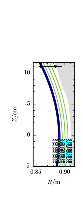
Figure 1: A poloidal cross-section of Alcator C-Mod’s outboard mid-plane section showing the last closed flux surface (LCFS) (purple line), magnetic flux surfaces in the SOL (green lines), the views of the APDs (cyan dots, red dots show the diode views used in this study), the trajectory of the MLP when scanning (black arrow) and the position where the MLP dwells during discharge 3 (green dot).

II.1 Calculation of synthetic gas-puff imaging data

Gas puff imaging diagnostics are routinely used to measure and visualize fluctuations of the boundary plasma. As realized on Alcator C-Mod, GPI utilizes a vertical stack of 4 “barrels“, located approximately $1.5\,\mathrm{cm}$ beyond the outermost column of views, see fig. 1, to puff a contrast gas into the boundary plasma. The line emission arising from the interaction between the gas atoms and the plasma are captured by a telescope whose optical axis is approximately toroidal and views the puff with sight lines that are approximately normal to the $(R,Z)$-plane at the toroidal angle of the nozzle. A fiber optic carries the light imaged by the telescope to a $9$ by $10$ array of avalanche photo diodes which sample it at $2\,\mathrm{MHz}$ (Cziegler et al., 2010).

The line emission intensity is related to the electron density $n_{\mathrm{e}}$ and temperature $T_{\mathrm{e}}$ as

$$I =n_{0}f(n_{\mathrm{e}},T_{\mathrm{e}}).$$ (1)

Here, $n_{0}$ is the puffed neutral gas density, $n_{\mathrm{e}}$ is the electron density and $T_{\mathrm{e}}$ is the electron temperature. The function $f$ parameterizes the ratio of the density of particles in the upper level of the radiative emission to the ground state density times the rate of decay of the upper level. As discussed in a review by Zweben et al. (2017), $f$ has been characterized by a power law dependence on the electron density and temperature for perturbations around values of $\langle n_{\mathrm{e}}\rangle$ and $\langle T_{\mathrm{e}}\rangle$ as

$$f(n_{\mathrm{e}},T_{\mathrm{e}})=n_{\mathrm{e}}^{\alpha}T_{\mathrm{e}}^{\beta}.$$ (2)

The exponents $\alpha$ and $\beta$ also depend on the gas species. Typical values of the fluctuating plasma parameters in the Alcator C-Mod SOL are given by $5\times 10^{18}\,\mathrm{m}^{-3}\lesssim n_{\mathrm{e}}\lesssim 5\times 10^{19}\,\mathrm{m}^{-3}$ and $10\,\mathrm{eV}\lesssim T_{\mathrm{e}}\lesssim 100\,\mathrm{eV}$ (Labombard et al., 1997; LaBombard et al., 2001, 2004; Kube et al., 2018b, 2019).

For this parameter range the exponents for HeI are within the range $0.2\lesssim\alpha\lesssim 0.8$ and $-0.4\lesssim\beta\lesssim 1.0$. Referring to Figure $7$ in Zweben et al. (2017) we note that in this parameter range $\alpha$ decreases monotonously with $n_{\mathrm{e}}$ while it varies little with $T_{\mathrm{e}}$ and that $\beta$ decreases monotonically with $T_{\mathrm{e}}$ while it varies little with $n_{\mathrm{e}}$. Most importantly, $f$ is approximately linear in $n_{\mathrm{e}}$ and $T_{\mathrm{e}}$ for small $n_{\mathrm{e}}$ and $T_{\mathrm{e}}$ while $f$ becomes less sensitive to $n_{\mathrm{e}}$ and $T_{\mathrm{e}}$ as they increase.

Equation 1 relates the measured line emission intensity to the plasma parameters and is subject to several assumptions. First, the radiative decay rate needs to be faster than characteristic time scales of the plasma fluctuations, neutral particle transport, and other atomic physics processes. For the He I $587\,\mathrm{nm}$ line, the radiative decay rate is given by the Einstein coefficient $A\approx 2\times 10^{7}\,\mathrm{s}^{-1}$, while the turbulence time scale is approximately $10\,\mu\mathrm{s}$. Second, $n_{0}$ is assumed to be slowly varying in time so that all fluctuations in $I$ can be ascribed to fluctuations in $n_{\mathrm{e}}$ and $T_{\mathrm{e}}$.

A synthetic line emission intensity signal is constructed using the emission rate $f$ for the $587\,\mathrm{nm}$ line of HeI, as calculated in the DEGAS2 code (Stotler & Karney, 1994), and using the $n_{\mathrm{e}}$ and $T_{\mathrm{e}}$ data time-series, as reported by the MLP:

$$I_{\mathrm{syn}}=f(n_{\mathrm{e}},T_{\mathrm{e}}).$$ (3)

Comparing this expression to Eq. 1, we note that the puffed-gas density $n_{0}$ is assumed to be constant and absorbed into $I_{\mathrm{syn}}$. This method for constructing synthetic GPI emissions is also used in Stotler et al. (2003); Halpern et al. (2015).

II.2 Calculation of profiles

The fluctuations of the plasma parameters can be characterized by their lower order statistical moments, that is, the mean, standard deviation, skewness and excess kurtosis. Scanning the Langmuir probe through the scrape-off layer yields a set of $I_{\mathrm{s}}$, $n_{\mathrm{e}}$, and $T_{\mathrm{e}}$ samples within a given radial interval along the scan-path. Here $I_{\mathrm{s}}$ is the ion saturation current. The center of the sampled interval is then mapped to the outboard mid-plane and assigned a $\rho_{\mathrm{mid}}$ value, corresponding to the distance from the last-closed flux surface. The number of samples within a given interval depends on the velocity with which the probe moves through the scrape-off layer as well as the width chosen for the sampling interval. Here, we use only data from the last two probe scans of discharge $1$ and $2$, as to sample data when the plasma SOL was stable in space and time.

The $n_{\mathrm{e}}$ and $T_{\mathrm{e}}$ data reported by the MLP are partitioned into separate sets for each instance, where the probe is within $\rho_{\mathrm{mid}}\pm\triangle_{\rho}$, that is, individually for the inward and outward part motion and individually for each probe plunge. Thus, for two probe plunges there are four datasets for $n_{\mathrm{e}}$ and $T_{\mathrm{e}}$ respectively. The lowest order statistical moments are calculated from the union of these data sets. To estimate the probability distribution function, the data time series are normalized by subtracting their sample mean and scaling with their respective root-mean-square value. This procedure was chosen to account for variations in the SOL plasma on a time scale comparable to the probe reciprocation time scale and the delay between consecutive probe plunges. Radial profiles of the lowest order statistical moments of the GPI data can be calculated using the time series of signals from the individual views.

Skewness $S$ and excess kurtosis $F$ of a data sample are invariant under linear transformations. In order to remove low-frequency trends in the data time series, for example due to shifts in the position of the last closed flux surface, $S$ and $F$ are calculated after normalizing the data samples according to

$$\widetilde{\Phi}=\frac{\Phi-\langle\Phi\rangle}{\Phi_{\mathrm{rms}}}.$$ (4)

Here $\langle\Phi\rangle$ denotes a running average and $\Phi_{\mathrm{rms}}$ the running root mean square value. This common normalization allows to compare the statistical properties of the fluctuations around the mean for different data time series using different diagnostic techniques. In the remainder of this article, all data time series are normalized according to Eq. 4.

II.3 Parameter estimation

It has been shown previously that measurement time series of the scrape-off layer plasma can be modeled accurately as the super-position of uncorrelated, two-sided exponential pulses. In the following we discuss how the intermittency parameter $\gamma$, the pulse duration time $\tau_{\mathrm{d}}$, the pulse asymmetry parameter $\lambda$, and the average waiting time between two consecutive pulses $\langle\tau_{\mathrm{w}}\rangle$ are reliably estimated.

The intermittency parameter $\gamma$ is obtained by fitting Equation (A9) in Theodorsen et al. (2017b) on the histogram of the measured time-series data, minimizing the logarithm of the squared residuals. The power spectral density (PSD) for a time series that results from the superposition of uncorrelated exponential pulses is given by Garcia & Theodorsen (2017),

$$\Omega_{\widetilde{\Phi}}(\omega) =\frac{2\tau_{\mathrm{d}}}{\left[1+\left(1-\lambda\right)^{2}\left(\tau_{\mathrm{d}}\omega\right)^{2}\right]\left[1+\lambda^{2}\left(\omega\tau_{\mathrm{d}}\right)^{2}\right]}.$$ (5)

Here $\tau_{\mathrm{d}}$ denotes the pulse duration time and $\lambda$ denotes the pulse asymmetry. The e-folding time of the pulse rise is then given by $\lambda\tau_{\mathrm{d}}$ and the e-folding time of the pulse decay is given by $\left(1-\lambda\right)\tau_{\mathrm{d}}$. We note that the PSD of the entire signal is the same as the PSD of a single pulse. The PSD has a Lorentzian shape, featuring a flat part for low frequencies and a power-law decay for high frequencies. The point of transition between these two regions is parameterized by $\tau_{\mathrm{d}}$ and the width of the transition region is given by $\lambda$. Note that for very small values of $\lambda$ the power law scaling can be further divided into a region where the PSD decays quadratically and into a region where the PSD decays as $\left(\tau_{\mathrm{d}}\omega\right)^{-4}$ (Garcia & Theodorsen, 2017). For the data at hand, power spectral densities are calculated using Welch’s method. This requires long data time series, which excludes data from scanning MLP operation.

Data from the MLP are pre-processed by applying a 12-point boxcar window to the data (Labombard & Lyons, 2007). Assuming that the pulse shapes in the time series of plasma parameters are well described by a two-sided exponential function, the MLP registers such pulses as just this pulse shape filtered with a boxcar window. Since the power spectral density of a superposition of uncorrelated pulses, i.e. the time series of the plasma parameters, is given by the power spectral density of an individual pulse (Garcia & Theodorsen, 2017), the expected power spectrum of MLP data time series is given by the product of Eq. 5 and the Fourier transformation of a boxcar window:

$$\Omega_{\widetilde{\Phi},\mathrm{MLP}}(\omega)=\Omega_{\widetilde{\Phi}}(\omega)\times\left[\frac{1}{6\triangle_{\text{t}}\omega}\sin\left(6\triangle_{\text{t}}\omega\right)\right]^{2}$$ (6)

To estimate the duration time $\tau_{\mathrm{d}}$ and pulse asymmetry parameter $\lambda$, Eq. 5 is used to fit the GPI data and Eq. 6 is used to fit the MLP data.

In order to get precise waiting time statistics and the a best estimate of $\tau_{\mathrm{w}}$, a method based on Richardson-Lucy (RL) deconvolution is used (Richardson, 1972; Lucy, 1974). This method was previously used for a comparison of GPI data from several different confinement modes in Alcator C-Mod. The method is described in more detail in Theodorsen et al. (2018), here we briefly describe the deconvolution.

By assuming that the dwell MLP and single-diode GPI signals are comprised by a series of uncorrelated pulses with a common pulse shape $\phi$ and a fixed duration $\tau_{\mathrm{d}}$, the signals can be written as a convolution between the pulse shape and a train of delta pulses,

$$\Phi(t)=\left[\phi*f\right]\left(\frac{t}{\tau_{\mathrm{d}}}\right),$$ (7)

where

$$f(t)=\sum_{k=1}^{K(T)}A_{k}\delta\left(\frac{t-t_{k}}{\tau_{\mathrm{d}}}\right).$$ (8)

The signal $\Phi$ can be seen as a train of delta pulses arriving according to a Poisson process $f$, passed through a filter $\phi$. It is therefore called a filtered Poisson process (FPP). For a prescribed pulse shape $\phi$ and a time series measurement of $\Phi$, the RL-deconvolution can be used to estimate $f$, that is, the pulse amplitudes $A_{\mathrm{k}}$ and arrival times $t_{\mathrm{k}}$. From the estimated forcing $f$, the waiting time statistics can be extracted. The RL-deconvolution is a point-wise iterative procedure which is known to converge to the least-squares solution (Dell’Acqua et al., 2007). For measurements with normally distributed measurement noise, the $n+1$’th iteration is given by (Daube-Witherspoon & Muehllehner, 1986; Pruksch & Fleischmann, 1998; Dell’Acqua et al., 2007; Tai et al., 2011)

$$f^{(n+1)}(t)=f^{(n)}(t)\frac{\left[\Phi*\widehat{\phi}\right](t)}{\left[f^{(n)}*\phi*\widehat{\phi}\right](t)},$$ (9)

where $\widehat{\phi}(t)=\phi(-t)$. For non-negative $\Phi$ and $f^{(0)}$, each following iteration will be non-negative as well. The initial choice $f^{(0)}$ is otherwise unimportant, and has here been set at constant unity. For consistency with PSD estimates of $\tau_{\mathrm{d}}$ and $\lambda$ (see Sec. III), we use a two-sided exponential pulse function with $\tau_{\mathrm{d}}=20\,\mu\text{s}$ and $\lambda=1/10$ for the GPI data, and a two-sided exponential pulse function with $\tau_{\mathrm{d}}=10\,\mu\text{s}$ and $\lambda=1/25$ convolved with the 12-point window for the MLP data. The deconvolution procedure is robust to small deviations in the pulse shape.

The deconvolution algorithm was run for $10^{5}$ iterations, after which the L²-difference between the measured time series and the reconstructed time series was considered sufficiently small. The result of the deconvolution resembles a series of sharply localized, Gaussian pulses, so a peak-finding algorithm is employed in order to extract pulse arrival times and amplitudes from the deconvolved signal. The window size of the peak finding algorithm is chosen to give the best fit to the expected number of events in the time series, resulting in window sizes of $7.5\,\mu\mathrm{s}$ ($I_{\mathrm{s}}$), $0.9\,\mu\text{s}$ ($n_{\mathrm{e}}$), $6.3\,\mu\text{s}$ ($T_{\mathrm{e}}$), $4.5\,\mu\text{s}$ (GPI, for the view at $90.7\,\text{cm}$) and $7.5\,\mu\text{s}$ (GPI, for the view at $91\,\text{cm}$). The deconvolution procedure finds $85001$, $200332$, $101815$, $30574$ and $17343$ pulses in these time series, respectively.

In order to test the fidelity of the process, a synthetic time series consisting of a pure FPP has been subjected to the deconvolution procedure as well. This time series has the same sampling time, $\tau_{\mathrm{d}}$ and $\lambda$ as the GPI time series, with $\gamma=2$. In this case, a window of $5.5\,\mu\text{s}$ gives the best fit to the expected number of events and the procedure finds 48011 events (the true number of events in the synthetic time series is 50000).

Example excerpts of the reconstructed time series are presented in Figs. 2 and 3. In both figures, the blue lines give the original time series, normalized according to Eq. 4. The green dots indicate the pulse arrival times and amplitudes which are the output of the deconvolution procedure described above. The amplitudes have been normalized by their own mean value and standard deviation. By convolving the estimated train of delta pulses with the pulse shape, the full time series is reconstructed. The result of this reconstruction is given by the orange lines. Overall, the reconstruction is excellent.

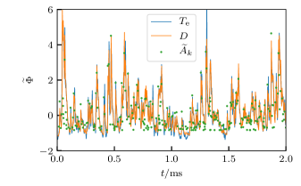
Figure 2: Excerpt of original (as measured by the MLP) and reconstructed $T_{\mathrm{e}}$ signals. The blue curve gives the original signal $T_{\mathrm{e}}$, the green dots indicate arrival times $t_{\mathrm{k}}$ and normalized amplitudes for the pulses $A_{\mathrm{k}}$ and the orange curve gives the reconstructed signal $D$. All signals are normalized such as to have zero mean and unit standard deviation.

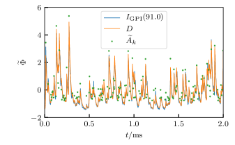
Figure 3: Excerpt of original and reconstructed GPI signals at $R=91\,\text{cm}$. The blue curve gives the original signal $I_{\mathrm{GPI}}$, the green dots indicate arrival times $t_{\mathrm{k}}$ and normalized amplitudes $A_{\mathrm{k}}$ for the pulses and the orange curve gives the reconstructed signal $D$. All signals are normalized such as to have zero mean and unit standard deviation.

III Results

III.1 Statistical properties of synthetic GPI intensity

Synthetic GPI emission rates are calculated according to Eq. 3, using data reported from the MLP in discharges 1 and 2. Figure 4 color codes the emission intensity given by Eq. 2 with data reported by the MLP overlaid. Discharge 1 features a scrape-off layer that is colder and less dense than the SOL plasma in discharge 2. Furthermore, the gradient scale-lengths of the $\langle n_{\mathrm{e}}\rangle$ and $\langle T_{\mathrm{e}}\rangle$ profiles are shorter in discharge 1 (Kube et al., 2019). Thus, the range of reported $n_{\mathrm{e}}$ and $T_{\mathrm{e}}$ values in discharge 1 (black markers) is larger than the range reported in discharge 2 (white markers). The contour lines suggest that both $\partial I_{\mathrm{syn}}/\partial T_{\mathrm{e}}$ and $\partial I_{\mathrm{syn}}/\partial n_{\mathrm{e}}$ are larger over the parameter range relevant for discharge 1 than they are for discharge 2. Consequently, variations in the amplitude of the plasma parameters $n_{\mathrm{e}}$ and $T_{\mathrm{e}}$ are mapped in a non-linear way to variations in the amplitude of $I_{\mathrm{syn}}$ and the local fluctuation exponents $\alpha$ and $\beta$ can not be used. Appendix A gives a more detailed discussion regarding the local exponent approximation.

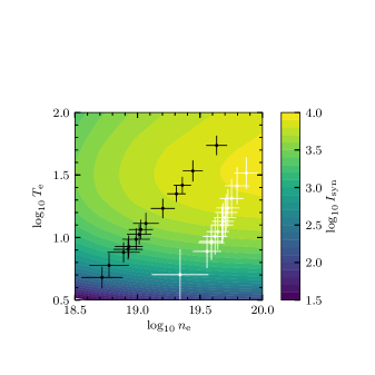
Figure 4: Synthetic emission rate for the HeI $587\,\mathrm{nm}$ line as a function of the electron density and temperature. Overplotted are the average $n_{\mathrm{e}}$ and $T_{\mathrm{e}}$ values reported by the MLP at different $\rho$ positions in discharge 1 (black markers) and 2 (white markers). The error bars are given by the respective root-mean-square values.

We now compare the lowest-order statistical moments of the different signals. Figure 10 shows radial profiles of the mean, the relative fluctuation level, skewness and intermittency parameter for the relevant MLP data ($n_{\mathrm{e}}$, $T_{\mathrm{e}}$, and $I_{\mathrm{s}}$), the GPI data, as well as the synthetic GPI data ($I_{\mathrm{syn}}$). Looking at the profile of the average values of $n_{\mathrm{e}}$ and $T_{\mathrm{e}}$, shown in 10 we note that the scale lengths of both quantities is almost identical. Both $n_{\mathrm{e}}$ and $T_{\mathrm{e}}$ decay sharply for $\rho\lesssim 1\,\mathrm{cm}$. With larger distance from the LCFS their profiles feature a larger scale length. Both MLP and GPI data feature a fluctuation level of up to $0.5$ times their respective mean. This relative fluctuation level increases with distance from the LCFS. The relative fluctuation level of the $I_{\mathrm{syn}}$ data also increases with $\rho$ but is less than the fluctuation level of the GPI data (by factors of $\sim 0.85$ and $\sim 0.3$) over the profile. Coefficients of sample skewness for the MLP and the GPI data are positive, comparable in magnitude and increase with $\rho$. The synthetic data features negative sample skewness for $\rho\lesssim 1\,\mathrm{cm}$ but are positive and increasing for $\rho\gtrsim 1\,\mathrm{cm}$. For both, MLP and GPI data, $F$ increases from approximately $0$ at $\rho\approx 0.5\,\mathrm{cm}$ to larger positive values for $\rho\approx 1.5\mathrm{cm}$. $F$ calculated using $I_{\mathrm{syn}}$ data is approximately zero over the entire range of $\rho$. The lowest panel of Fig. 10 shows the intermittency parameter $\gamma$, obtained by a fit on the histogram of data sampled in a given $\rho$ bin. Both, MLP and GPI data feature a large value of $\gamma\gtrsim 10$ for $\rho\lesssim 1\mathrm{cm}$. This implies that the PDFs closely follow a normal distribution, which is consistent with small values of $S$ and $F$. For larger $\rho$ values the data features positively skewed and flattened histograms, a feature captured by the smaller $\gamma$ value and compatible with the larger estimates of $S$ and $F$. For the synthetic data, $\gamma$ is estimated to be larger than $10$ over the entire range of $\rho$. This implies that these samples closely follow a normal distribution, which is compatible with nearly vanishing skewness and excess kurtosis of this data.

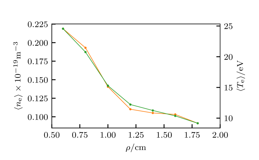
Figure 5: Average

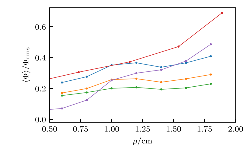
Figure 6: Relative fluctuation level

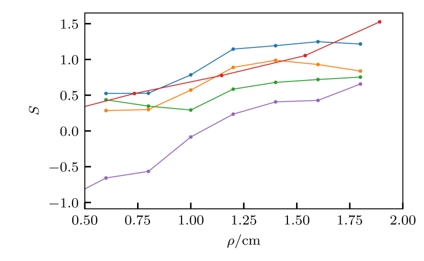
Figure 7: Skewness

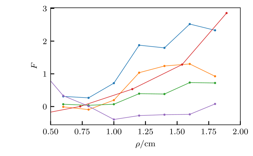
Figure 8: Relative fluctuation level

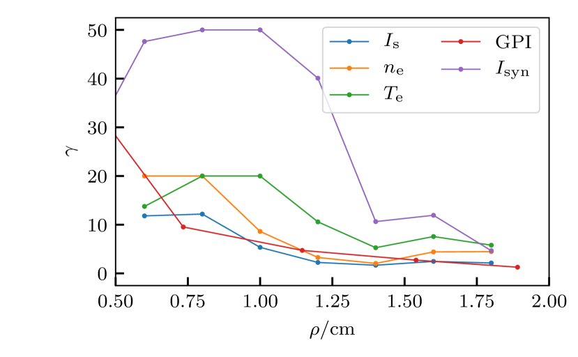
Figure 9: Intermittency parameter

Figure 10: Radial profiles of various quantities sampled in discharge 1. The color legend in subplot 10 applies to all subplots.

While the radial profiles of the lowest order statistical moments calculated using MLP and GPI data agree qualitatively the profiles of the $I_{\mathrm{syn}}$ data show large discrepancies. The relative fluctuation level of the $I_{\mathrm{syn}}$ data is comparable to the relative fluctuation level of the $I_{\mathrm{s}}$, $n_{\mathrm{e}}$, $T_{\mathrm{e}}$ and the GPI data, while $S$, $F$, and $\gamma$ calculated using $I_{\mathrm{syn}}$ data correspond to a near-gaussian process. Fig. 11 shows $n_{\mathrm{e}}$, $T_{\mathrm{e}}$ and $I_{\mathrm{syn}}$ time series. The waveforms of the $n_{\mathrm{e}}$ and $T_{\mathrm{e}}$ data present intermittent and asymmetric large-amplitude bursts for both discharge 1 and 2. Peaks in the $I_{\mathrm{syn}}$ on the other hand appear with a somewhat smaller amplitude relative to the quiet time between bursts and with a more symmetric shape. Histograms of the corresponding data, shown in Fig. 12, corroborate this interpretation. For the data sampled in discharge 1 (full lines in Fig. 11 and the left panel in Fig. 12), histograms of the $n_{\mathrm{e}}$ and $T_{\mathrm{e}}$ data are asymmetric with elevated tails for large-amplitude events. The histogram of the $I_{\mathrm{syn}}$ data on the other hand features no elevated tail for large amplitude events. For $\widetilde{I}_{\mathrm{syn}}\gtrsim 2.5$ the histogram is approximately zero. For discharge 2 (dashed lines in Fig. 11 and the right panel in Fig. 12), the histogram of the $I_{\mathrm{syn}}$ data appears symmetric and features a plateau around $\widetilde{I}_{\mathrm{syn}}=0$ without a pronounced peak.

The different fluctuation statistics can be understood by referring to Fig. 4. For one, $I_{\mathrm{syn}}$ is more sensitive to $T_{\mathrm{e}}$ fluctuations than to $n_{\mathrm{e}}$ fluctuations, that is, $\partial I_{\mathrm{syn}}/\partial T_{\mathrm{e}}>\partial I_{\mathrm{syn}}/\partial n_{\mathrm{e}}$ within relevant ranges of $n_{\mathrm{e}}$ and $T_{\mathrm{e}}$. Furthermore, both scaling exponents $\alpha$ and $\beta$ may vary significantly over the range of a single large-amplitude burst, as indicated by the error bars. Since $n_{\mathrm{e}}$ and $T_{\mathrm{e}}$ fluctuations are strongly correlated and feature similar pulse shapes (Kube et al., 2018b), Eq. 3 does not result in a perfectly scaled pulse shape of the input signals. For example, when assuming a two-sided exponential pulse for $n_{\mathrm{e}}$ and $T_{\mathrm{e}}$ as input for Eq. 3, the resulting pulse shape is not a two-sided exponential pulse, but rather a boxcar-like pulse as the saturation levels of $n_{\mathrm{e}}$ and $T_{\mathrm{e}}$ are reached.

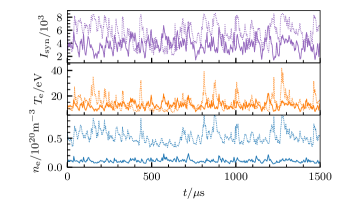
Figure 11: Time series of $n_{\mathrm{e}}$ (lowest panel), $T_{\mathrm{e}}$ (middle panel), and synthetic GPI data (top panel) for discharge 1 (full line) and 2 (dashed line). Data are taken in the first interval where the probe scans from $\rho=1.3$ to $1.2\,\mathrm{cm}$.

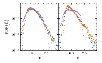
Figure 12: Histogram of $\widetilde{n}_{\mathrm{e}}$ (blue dots), $\widetilde{T}_{\mathrm{e}}$ (orange dots), and $\widetilde{I}_{\mathrm{syn}}$ (purple dots) for discharge 1 (left) and 2 (right). Data are taken in all intervals where the probe scans from $\rho=1.2$ to $1.3\,\mathrm{cm}$.

III.2 Statistical properties of MLP and GPI data

Figure 13 shows the frequency power spectral densities calculated from MLP and GPI data sampled in discharge 3. The PSDs of the GPI data from the different radial positions, shown in the left panel, are almost identical. They are flat for low frequencies, $f\lesssim 5\,\mathrm{kHz}$, before transitioning into a broken power law decay for high frequencies. A least squares fit of Eq. 5 on the data (black line) yields $\tau_{\mathrm{d}}=20\,\mu\mathrm{s}$ and $\lambda\approx 0.1$ and describes the PSDs of the signals perfectly over more than 4 decades.

PSDs of the MLP data ($I_{\mathrm{s}}$, $n_{\mathrm{e}}$, and $T_{\mathrm{e}}$) appear similar in shape to the PSD of the GPI data, except that for high frequencies, $f\gtrsim 0.2\,\mathrm{MHz}$, a “ringing” effect can be observed. This is due to internal data processing of the MLP, which smooths data with a 12-point uniform filter as discussed above (Kube et al., 2018b). Fitting Eq. 6 on the data yields $\tau_{\mathrm{d}}=10\,\mu\mathrm{s}$ and $\lambda=0.04$. The red and black line in the right-hand panel show Eq. 6 and Eq. 5 respectively with these parameters. While Eq. 6 describes the Lorentzian-like decay of the experimental data as well as the ”ringing” effect at high frequencies, it underestimates the low frequency part of the spectrum, $f\lesssim 10^{-2}\,\mathrm{MHz}$. This is addressed by the deconvolution procedure.

Summarizing the parameters found by fitting the GPI and MLP data, we find $\tau_{\mathrm{d}}=20\,\mu\mathrm{s}$ and $\lambda=1/10$ for GPI data and $\tau_{\mathrm{d}}=10\,\mu\mathrm{s}$ and $\lambda=1/25$ for MLP data. In other words, the MLP observes shorter pulses that are more asymmetric than the GPI. Since the GPI measures light emissions from a finite volume (that is at least the 4 mm diameter spot-size times the toroidal extent of the gas cloud) and pulses in the signal are due to radially- or poloidally- propagating blob structures, it can be expected that the registered pulses in the signal appear more smeared out, compared to those from the Langmuir probes, which measure plasma parameters at the probe tips. No such “pulse smearing” pollutes the MLP signals. This may be the reason for the difference found for the $\tau_{\mathrm{d}}$ and $\lambda$ parameters.

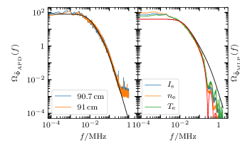
Figure 13: The left panel shows the PSD of the GPI data from discharge 3 and Eq. 5 using parameters from a least-squares fit. The right panel shows PSDs of the MLP signals and both, Eq. 6 (red line) and Eq. 5 (black line) evaluated using parameters found from a least-squares fit.

Figs. 14 - Fig. 16 show the results of the deconvolution procedure, starting with the PDF of the waiting times. The brown triangles give the estimated waiting times of the synthetically generated signal, while the black dotted line indicates an exponential decay. The GPI waiting time distribution conforms very well to the exponential decay of the synthetic time series for the entire distribution. The MLP waiting time distributions decay exponentially over at least two decades in probability. All waiting time distributions have lower probability of small waiting times ($\tau_{\mathrm{w}}/\langle\tau_{\mathrm{w}}\rangle\lesssim 0.8$) compared to an exponential distribution, an artifact of the non-zero $\tau_{\mathrm{d}}$ and the peak finding algorithm. This is also true for the synthetic time series.

Fig. 15 shows the PDF of the pulse amplitudes obtained by applying the deconvolution procedure. The pulse amplitudes are approximately exponentially distributed for all analyzed signals. The $n_{\mathrm{e}}$ data and the synthetic GPI data both appear sub-exponential. On the other hand, the distribution of pulse amplitudes both GPI data time series appears to be identical to the distribution reconstructed from the $I_{\mathrm{s}}$ and $T_{\mathrm{e}}$ data. For small and large amplitudes, the plotted PDFs show deviations from an exponential function. The deviation for large amplitudes is due to the finite size of the data time series. Deviations for small amplitudes are also observed in other measurement data (Theodorsen et al., 2018).

In Fig. 16, the autocorrelation function of the consecutive waiting times is presented. Here, $R_{\widetilde{\tau}_{\text{w}}}[n]=R_{\widetilde{\tau}_{\text{w}}}[k,k+n]=\langle\widetilde{\tau}_{\text{w},k}\,\widetilde{\tau}_{\text{w},k+n}\rangle$, and $\tau_{\text{w}}$ is normalized by subtracting its mean value and dividing by its standard deviation. This function is very close to a delta function, indicating that consecutive pulses are uncorrelated and thus supporting the assumptions of pulses arriving according to a Poisson process.

Together, these results indicate that the waiting times derived from the GPI and MLP data follow the same distribution and are consistent with exponentially distributed and independent waiting times. This further justifies using the stochastic model framework. The estimated average waiting times are presented in Tab. 2, and give $\gamma$-values consistent with those obtained from fits to the histograms of the time series.

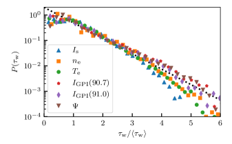
Figure 14: Probability density functions of waiting times obtained from deconvolving the GPI and MLP time series. The synthetically generated time series is indicated by $\Psi$. The black dotted line indicates exponential decay.

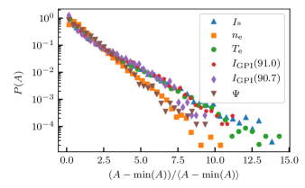
Figure 15: Probability density functions of the pulse amplitudes obtained from deconvolving the GPI and MLP time series. The synthetically generated time series is indicated by $\Psi$.

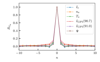
Figure 16: Auto-correlation functions of the waiting times obtained from the deconvolution procedure. Here, $n$ gives the number of waiting times away from the reference waiting time. The synthetically generated time series is indicated by $\Psi$.

The discrepancy between the low-frequency prediction of Eq. 5 and the PSD of the MLP data is resolved by the deconvolution procedure. In Fig. 17, the power spectral densities of the MLP data time series are presented together with the power spectral densities of the reconstructed time series and the analytic prediction. The reconstructed time series give the same behavior for low frequencies as the MLP data, showing that this discrepancy is explainable by the synthetic time series.

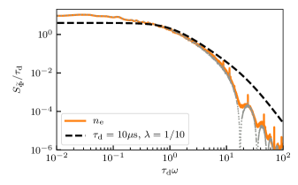
Figure 17: Full line: Power spectral densities of MLP time series. Dotted line: Reconstructed time series from the RL-deconvolution. The black dashed line gives the power spectral density predicted by Eq. 5 for the two-sided exponential pulse.

parameter	method	$I_{\mathrm{s}}$	$n_{\mathrm{e}}$	$T_{\mathrm{e}}$	GPI $90\,cm$	GPI $91\,cm$
$\gamma$	PDF fit	1.01	3.22	1.33	3.54	2.01
$\langle\tau_{\mathrm{w}}\rangle/\mu\mathrm{s}$	RL deconv	8.6	3.3	7.1	4.7	9.0
$\tau_{\mathrm{d}}/\mu\mathrm{s}$	PSD fit	9.2	9.7	9.8	19.7	19.1
$\gamma$	$\tau_{\mathrm{{d}}}/\langle\tau_{\mathrm{{w}}}\rangle$	${1.1}$	${2.96}$	${1.39}$	${4.20}$	${2.12}$

Table 2: Process and pulse parameters estimated using MLP and GPI data sampled in discharge 3.

Table 2 summarizes the parameter estimation. The first three rows list the parameters estimated using the methods described above. For the $I_{\mathrm{s}}$ and $T_{\mathrm{e}}$ data, we find $\gamma\approx 1$. This describes a strongly intermittent time series with significant quiet time in between pulses. For the $n_{\mathrm{e}}$ time series we find $\gamma\approx 3.2$, comparable to the estimates for the GPI data. The average waiting time between pulses is $\langle\tau_{\mathrm{w}}\rangle\approx 8\,\mu\mathrm{s}$. The best estimate for $\langle\tau_{\mathrm{w}}\rangle$ from the $n_{\mathrm{e}}$ time series is given by $\langle\tau_{\mathrm{w}}\rangle\approx 3.3\,\mu\mathrm{s}$, estimates from the GPI data are larger by a factor of $2-3$, depending on the radial position of the view. The pulse duration time for the MLP data is $\tau_{\mathrm{d}}\approx 10\,\mu\mathrm{s}$, smaller by a factor of two than for the GPI data, probably for the reasons discussed above.

The bottom row lists the intermittency parameter calculated using the estimated pulse duration time and average waiting time, $\gamma=\tau_{\mathrm{d}}/\langle\tau_{\mathrm{w}}\rangle$. The deconvolution algorithm uses $\tau_{\mathrm{d}}$ from the power spectrum as an input parameter and $\gamma$ from the PDF fit as a constraint. Therefore, the fact that $\tau_{\mathrm{d}}/\langle\tau_{\mathrm{w}}\rangle$ is comparable to $\gamma$ estimated from the PDF fit is a good consistency check.

IV Conclusions and summary

Fluctuations of the scrape-off layer plasma have been studied for a series of ohmically heated discharges in Alcator C-Mod. It is found that the radial variations of the lowest order statistical moments, calculated from MLP and GPI measurements, are quantitatively similar. Time series data from both MLP and GPI diagnostics, feature intermittent, large-amplitude bursts. As shown in numerous previous publications, the time series are well described as a superposition of uncorrelated pulses with a two-sided exponential pulse shape and a pulse amplitude that closely follows an exponential distribution. In this contribution we demonstrate that the parameters which describe the various parameters of the stochastic process agree across MLP and GPI diagnostics. In particular, the same statistical properties apply to the ion saturation current, electron density and temperature, and the line emission intensity.

Radial profiles of the relative fluctuation level, skewness, and excess kurtosis, as estimated from both MLP and GPI data, are of similar magnitude and are monotonically increasing with distance from the LCFS. This holds regardless of using $I_{\mathrm{s}}$, $n_{\mathrm{e}}$ or $T_{\mathrm{e}}$ from the MLP. For the GPI data the time series feature an intermittency parameter $\gamma\approx 2-3$, when estimated from a fit on the PDF. Estimating the intermittency parameter by a fit on the PDF of the different MLP data time series yields $\gamma\approx 3$ for the $n_{\mathrm{e}}$ data and $\gamma\approx 1$ for both the $I_{\mathrm{s}}$ and $T_{\mathrm{e}}$ data. Pulse duration times, estimated from fits on the time series frequency power spectral density, are $\tau_{\mathrm{d}}\approx 10\,\mu\mathrm{s}$ for all MLP data time series while we find $\tau_{\mathrm{d}}\approx 20\,\mu\mathrm{s}$ for the GPI data time series. This deviation by a factor of 2 is likely due to the relatively large in-focus spot size of the individual GPI views. Reconstructing the distributions of waiting times between consecutive pulses from a Richardson-Lucy deconvolution, yields average waiting times between pulses of $\langle\tau_{\mathrm{w}}\rangle\approx(3,7,9)\,\mu\mathrm{s}$ for the $(n_{\mathrm{e}},T_{\mathrm{e}},I_{\mathrm{s}})$ data. Using GPI data time series, we find $\langle\tau_{\mathrm{w}}\rangle\approx 5$ and $10\,\mu\mathrm{s}$ for the views at $R=90.7$ and $91.0\,\mathrm{cm}$ respectively. We note that the GPI view at $R=91.0\,\mathrm{cm}$ is close to the limiter shadow. Finally, estimating the intermittency parameter as $\tau_{\mathrm{d}}/\langle\tau_{\mathrm{w}}\rangle$ from the deconvolution of the time series gives almost the same values as estimating $\gamma$ by a fit on the PDF. These findings show that the model parameters of the stochastic model, $\gamma$, $\tau_{\mathrm{d}}$ and $\langle\tau_{\mathrm{w}}\rangle$, are indeed a good parameterization of the plasma fluctuations, independent of the diagnostic used to measure them. Reconstructing the arrival times and amplitude of the individual pulses using Richardson-Lucy deconvolution is an invaluable tool for obtaining the distribution of waiting times between consecutive pulses.

Our analysis also suggests that calculating a synthetic line emission signal using the instantaneous plasma parameters reported by the MLP results in a signal with different fluctuation statistics than the time series actually measured by the GPI. The synthetic data time series present intermittent pulses, but with a different shape than observed by the GPI. The PDF of these signals furthermore are close to a normal distribution, with low moments of skewness, excess kurtosis and no elevated tails. We hypothesize argued that ionization, where hot plasma filaments locally decrease the puffed gas density, is the main cause of this phenomenon and therefore should be accounted for in such an attempt to reproduce the emission from measurements of $n_{\mathrm{e}}$ and $T_{\mathrm{e}}$.

Having established $\gamma$, $\tau_{\mathrm{d}}$, and $\langle\tau_{\mathrm{w}}\rangle$ as consistent estimators for fluctuations in the scrape-off layer, future work will focus on describing their variations with plasma parameters.

V Acknowledgements

This work was supported with financial subvention from the Research Council of Norway under Grant No. 240510/F20 and the from the U.S. DoE under Cooperative Agreement No. DE-FC02-99ER54512 40 using the Alcator C-Mod tokamak, a DoE Office of Science user facility. A.T. and O.E.G. were supported by the UiT Aurora Centre for Nonlinear Dynamics and Complex Systems Modelling. R.K., O. E. G., and A. T.  acknowledge the generous hospitality of the MIT Plasma Science and Fusion Center during a research stay where part of this work was performed. J.L.T acknowledges the generous hospitality of UiT The Arctic University of Norway and its scientific staff during his stay there.

Appendix A Local and global fluctuations

The emission intensity, measured by GPI, is often parameterized as

$$I =n_{0}\times F\left(n_{\mathrm{e}},T_{\mathrm{e}}\right),$$ (10)

where $n_{0}$ is a constant neutral background density. Thus, the differential of $I$ can be written as

$$\frac{\mathrm{d}I}{I} =\frac{\partial\ln f}{\partial\ln n_{\mathrm{e}}}\frac{\mathrm{d}n_{\mathrm{e}}}{n_{\mathrm{e}}}+\frac{\partial\ln f}{\partial\ln T_{\mathrm{e}}}\frac{\mathrm{d}T_{\mathrm{e}}}{T_{\mathrm{e}}},$$ (11)

where we use the notation $\partial\ln f(x)/\partial\ln x=\left(x/f(x)\right)\partial f(x)/\partial x$. Assuming small fluctuation amplitudes, the differential of a function $u$ can be approximated as

$$\frac{\mathrm{d}u}{u}\approx\frac{\triangle u}{u}=\frac{u-\langle u\rangle}{\langle u\rangle+\triangle u}\approx\frac{u-\langle u\rangle}{\langle u\rangle}.$$ (12)

Here, $\triangle u$ is a small, but non-infinitesimal change in $u$ and $\langle u\rangle$ denotes an average. That is, the relative, infinitesimal change in a function $u$ is approximately the deviation of $u$ to an average $\langle u\rangle$ relative to this average. This approximation gives the local density and temperature exponents $\beta_{n}$ and $\alpha_{T}$:

$$\frac{I-\langle I\rangle}{\langle I\rangle}\approx\beta_{n}\frac{n_{\mathrm{e}}-\langle n_{\mathrm{e}}\rangle}{\langle n_{\mathrm{e}}\rangle}+\alpha_{T}\frac{T_{\mathrm{e}}-\langle T_{\mathrm{e}}\rangle}{\langle T_{\mathrm{e}}\rangle},$$ (13)

where $\beta_{n}=\partial\ln f/\partial\ln n_{\mathrm{e}}$ and $\alpha_{T}=\partial\ln f/\partial\ln T_{\mathrm{e}}$ at a given (fixed) $\langle n_{\mathrm{e}}\rangle$ and $\langle T_{\mathrm{e}}\rangle$.

For large deviations relative to the mean values, this local approximation breaks down for two reasons. First, the infinitesimal change $\text{d}u$ can no longer be approximated as a variation relative to a mean value. Second, the partial derivatives in Eq. 11, which are evaluated at a fixed point, are not necessarily constant when using non-infinitesimal values for the $\mathrm{d}n_{\mathrm{e}}$ or $\mathrm{d}T_{\mathrm{e}}$. The local exponents are therefore not constant, and the full, global Eq. 10 must be used.

References

- Adámek et al. (2004) Adámek, J., Stöckel, J., Hron, M., Ryszawy, J., Tichý, M., Schrittwieser, R., Ionită, C., Balan, P., Martines, E. & Oost, G. V. 2004 A novel approach to direct measurement of the plasma potential. Czechoslovak Journal of Physics 54 (3), C95.
- Banerjee et al. (2012) Banerjee, S., Zushi, H., Nishino, N., Hanada, K., Sharma, S., Honma, H., Tashima, S., Inoue, T., Nakamura, K., Idei, H., Hasegawa, M. & Fujisawa, A. 2012 Statistical features of coherent structures at increasing magnetic field pitch investigated using fast imaging in quest. Nuclear Fusion 52 (12), 123016.
- Boedo et al. (2014) Boedo, J. A., Myra, J. R., Zweben, S., Maingi, R., Maqueda, R. J., Soukhanovskii, V. A., Ahn, J. W., Canik, J., Crocker, N., D’Ippolito, D. A., Bell, R., Kugel, H., Leblanc, B., Roquemore, L. A., Rudakov, D. L. & Team, N. 2014 Edge transport studies in the edge and scrape-off layer of the national spherical torus experiment with langmuir probes. Physics of Plasmas (1994-present) 21 (4).
- Boedo et al. (2003) Boedo, J. A., Rudakov, D. L., Moyer, R. A., McKee, G. R., Colchin, R. J., Schaffer, M. J., Stangeby, P. G., West, W. P., Allen, S. L., Evans, T. E., Fonck, R. J., Hollmann, E. M., Krasheninnikov, S., Leonard, A. W., Nevins, W., Mahdavi, M. A., Porter, G. D., Tynan, G. R., Whyte, D. G. & Xu, X. 2003 Transport by intermittency in the boundary of the diii-d tokamak. Physics of Plasmas 10 (5), 1670–1677.
- Brunner et al. (2017) Brunner, D., Kuang, A. Q., LaBombard, B. & Burke, W. 2017 Linear servomotor probe drive system with real-time self-adaptive position control for the alcator c-mod tokamak. Review of Scientific Instruments 88 (7), 073501, arXiv: https://doi.org/10.1063/1.4990043.
- Carralero et al. (2014) Carralero, D., Birkenmeier, G., Müller, H., Manz, P., deMarne, P., Müller, S., Reimold, F., Stroth, U., Wischmeier, M., Wolfrum, E. & Team, T. A. U. 2014 An experimental investigation of the high density transition of the scrape-off layer transport in asdex upgrade. Nuclear Fusion 54 (12), 123005.
- Cziegler et al. (2010) Cziegler, I., Terry, J. L., Hughes, J. W. & LaBombard, B. 2010 Experimental studies of edge turbulence and confinement in alcator c-mod. Physics of Plasmas 17 (5), 056120.
- Daube-Witherspoon & Muehllehner (1986) Daube-Witherspoon, M. E. & Muehllehner, G. 1986 An Iterative Image Space Reconstruction Algorthm Suitable for Volume ECT. IEEE Trans. Med. Imaging 5 (2), 61–66.
- Dell’Acqua et al. (2007) Dell’Acqua, F., Rizzo, G., Scifo, P., Clarke, R. A., Scotti, G. & Fazio, F. 2007 A Model-Based Deconvolution Approach to Solve Fiber Crossing in Diffusion-Weighted MR Imaging. IEEE Trans. Biomed. Eng. 54 (3), 462–472.
- D’Ippolito et al. (2011) D’Ippolito, D. A., Myra, J. R. & Zweben, S. J. 2011 Convective transport by intermittent blob-filaments: Comparison of theory and experiment. Physics of Plasmas 18 (6), 060501.
- Endler et al. (1995) Endler, M., Niedermeyer, H., Giannone, L., Kolzhauer, E., Rudyj, A., Theimer, G. & Tsois, N. 1995 Measurements and modelling of electrostatic fluctuations in the scrape-off layer of asdex. Nuclear Fusion 35 (11), 1307.
- Fuchert et al. (2014) Fuchert, G., Birkenmeier, G., Carralero, D., Lunt, T., Manz, P., Müller, H. W., Nold, B., Ramisch, M., Rohde, V. & Stroth, U. 2014 Blob properties in l- and h-mode from gas-puff imaging in ASDEX upgrade. Plasma Physics and Controlled Fusion 56 (12), 125001.
- Garcia et al. (2017) Garcia, O., Kube, R., Theodorsen, A., Bak, J.-G., Hong, S.-H., Kim, H.-S., the KSTAR Project Team & Pitts, R. 2017 Sol width and intermittent fluctuations in kstar. Nuclear Materials and Energy 12, 36 – 43, proceedings of the 22nd International Conference on Plasma Surface Interactions 2016, 22nd PSI.
- Garcia (2012) Garcia, O. E. 2012 Stochastic modeling of intermittent scrape-off layer plasma fluctuations. Phys. Rev. Lett. 108, 265001.
- Garcia et al. (2013a) Garcia, O. E., Cziegler, I., Kube, R., LaBombard, B. & Terry, J. L. 2013a Burst statistics in alcator c-mod sol turbulence. Journal of Nuclear Materials 438, S180 – S183.
- Garcia et al. (2013b) Garcia, O. E., Fritzner, S. M., Kube, R., Cziegler, I., LaBombard, B. & Terry, J. L. 2013b Intermittent fluctuations in the alcator c-mod scrape-off layer. Phys. Plasmas 20, 055901.
- Garcia et al. (2015) Garcia, O. E., Horacek, J. & Pitts, R. A. 2015 Intermittent fluctuations in the tcv scrape-off layer. Nuclear Fusion 55 (6), 062002.
- Garcia et al. (2007) Garcia, O. E., Horacek, J., Pitts, R. A., Nielsen, A. H., Fundamenski, W., Naulin, V. & Rasmussen, J. J. 2007 Fluctuations and transport in the tcv scrape-off layer. Nuclear Fusion 47 (7), 667.
- Garcia et al. (2016) Garcia, O. E., Kube, R., Theodorsen, A. & Pécseli, H. L. 2016 Stochastic modelling of intermittent fluctuations in the scrape-off layer: Correlations, distributions, level crossings, and moment estimation. Physics of Plasmas 23 (5), 052308.
- Garcia & Theodorsen (2017) Garcia, O. E. & Theodorsen, A. 2017 Auto-correlation function and frequency spectrum due to a super-position of uncorrelated exponential pulses. Physics of Plasmas 24 (3), 032309.
- Graves et al. (2005) Graves, J. P., Horacek, J., Pitts, R. A. & Hopcraft, K. I. 2005 Self-similar density turbulence in the tcv tokamak scrape-off layer. Plasma Physics and Controlled Fusion 47 (3), L1.
- Greenwald (2002) Greenwald, M. 2002 Density limits in toroidal plasmas. Plasma Physics and Controlled Fusion 44 (8), R27.
- Grulke et al. (2014) Grulke, O., Terry, J. L., Cziegler, I., LaBombard, B. & Garcia, O. E. 2014 Experimental investigation of the parallel structure of fluctuations in the scrape-off layer of alcator c-mod. Nuclear Fusion 54 (4), 043012.
- Halpern et al. (2015) Halpern, F. D., Terry, J. L., Zweben, S. J., LaBombard, B., Podesta, M. & Ricci, P. 2015 Comparison of 3d flux-driven scrape-off layer turbulence simulations with gas-puff imaging of alcator c-mod inner-wall limited discharges. Plasma Physics and Controlled Fusion 57 (5), 054005.
- J. Horacek (2005) J. Horacek, R. A. Pitts, J. G. 2005 Overview of edge electrostatic turbulence experiments on tcv. Czechoslovak Journal of Physics 55 (3), 271–283.
- Kirnev et al. (2004) Kirnev, G. S., Budaev, V. P., Grashin, S. A., Gerasimov, E. V. & Khimchenko, L. N. 2004 Intermittent transport in the plasma periphery of the t-10 tokamak. Plasma Physics and Controlled Fusion 46 (4), 621.
- Kuang et al. (2019) Kuang, A. Q., LaBombard, B., Brunner, D., Garcia, O., Kube, R. & Theodorsen, A. 2019 Plasma fluctuations in the scrape-off layer and at the divertor target in alcator c-mod and their relationship to divertor collisionality and density shoulder formation. Nuclear Materials and Energy 19, 295 – 299.
- Kube et al. (2018a) Kube, R., Garcia, O. E., Theodorsen, A., Brunner, D., Kuang, A. Q., LaBombard, B. & Terry, J. L. 2018a Intermittent electron density and temperature fluctuations and associated fluxes in the alcator c-mod scrape-off layer. Plasma Physics and Controlled Fusion 60 (6), 065002.
- Kube et al. (2018b) Kube, R., Garcia, O. E., Theodorsen, A., Brunner, D., Kuang, A. Q., LaBombard, B. & Terry, J. L. 2018b Intermittent electron density and temperature fluctuations and associated fluxes in the alcator c-mod scrape-off layer. Plasma Physics and Controlled Fusion 60 (6), 065002.
- Kube et al. (2019) Kube, R., Garcia, O. E., Theodorsen, A., Kuang, A. Q., LaBombard, B., Terry, J. L. & Brunner, D. 2019 Statistical properties of the plasma fluctuations and turbulent cross-field fluxes in the outboard mid-plane scrape-off layer of alcator c-mod. Nuclear Materials and Energy 18, 193 – 200.
- Kube et al. (2016) Kube, R., Theodorsen, A., Garcia, O. E., LaBombard, B. & Terry, J. L. 2016 Fluctuation statistics in the scrape-off layer of alcator c-mod. Plasma Physics and Controlled Fusion 58 (5), 054001.
- LaBombard et al. (2001) LaBombard, B., Boivin, R. L., Greenwald, M., Hughes, J., Lipschultz, B., Mossessian, D., Pitcher, C. S., Terry, J. L., Zweben, S. J. & the Alcator C-Mod Group 2001 Particle transport in the scrape-off layer and its relationship to discharge density limit in alcator c-mod. Physics of Plasmas 8 (5), 2107–2117.
- Labombard et al. (1997) Labombard, B., Goetz, J., Hutchinson, I., Jablonski, D., Kesner, J., Kurz, C., Lipschultz, B., McCracken, G., Niemczewski, A., Terry, J., Allen, A., Boivin, R., Bombarda, F., Bonoli, P., Christensen, C., Fiore, C., Garnier, D., Golovato, S., Granetz, R., Greenwald, M., Horne, S., Hubbard, A., Irby, J., Lo, D., Lumma, D., Marmar, E., May, M., Mazurenko, A., Nachtrieb, R., Ohkawa, H., O’Shea, P., Porkolab, M., Reardon, J., Rice, J., Rost, J., Schachter, J., Snipes, J., Sorci, J., Stek, P., Takase, Y., Wang, Y., Watterson, R., Weaver, J., Welch, B. & Wolfe, S. 1997 Experimental investigation of transport phenomena in the scrape-off layer and divertor. Journal of Nuclear Materials 241–243 (0), 149 – 166.
- LaBombard et al. (2014) LaBombard, B., Golfinopoulos, T., Terry, J. L., Brunner, D., Davis, E., Greenwald, M. & Hughes, J. W. 2014 New insights on boundary plasma turbulence and the quasi-coherent mode in alcator c-mod using a mirror langmuir probe. Physics of Plasmas 21 (5), 056108.
- Labombard & Lyons (2007) Labombard, B. & Lyons, L. 2007 Mirror langmuir probe: A technique for real-time measurement of magnetized plasma conditions using a single langmuir electrode. Review of Scientific Instruments 78 (7), 073501–073501–9.
- LaBombard et al. (2004) LaBombard, B., Rice, J., Hubbard, A., Hughes, J., Greenwald, M., Irby, J., Lin, Y., Lipschultz, B., Marmar, E., Pitcher, C., Smick, N., Wolfe, S., Wukitch, S. & the Alcator Group 2004 Transport-driven scrape-off-layer flows and the boundary conditions imposed at the magnetic separatrix in a tokamak plasma. Nuclear Fusion 44 (10), 1047.
- Lao et al. (1985) Lao, L., John, H. S., Stambaugh, R., Kellman, A. & Pfeiffer, W. 1985 Reconstruction of current profile parameters and plasma shapes in tokamaks. Nuclear Fusion 25 (11), 1611.
- Lucy (1974) Lucy, L. B. 1974 An iterative technique for the rectification of observed distributions. Astron. J. 79, 745.
- Militello & Omotani (2016) Militello, F. & Omotani, J. 2016 Scrape off layer profiles interpreted with filament dynamics. Nuclear Fusion 56 (10), 104004.
- Pruksch & Fleischmann (1998) Pruksch, M. & Fleischmann, F. 1998 Positive Iterative Deconvolution in Comparison to Richardson-Lucy Like Algorithms. In Astron. Data Anal. Softw. Syst. VII (ed. Rudolf Albrecht, Richard N. Hook & Howard A. Bushouse), pp. 496–499. Astronomical Society of the Pacific Conference Series.
- Richardson (1972) Richardson, W. H. 1972 Bayesian-Based Iterative Method of Image Restoration*. J. Opt. Soc. Am. 62 (1), 55.
- Rudakov et al. (2002) Rudakov, D. L., Boedo, J. A., Moyer, R. A., Krasheninnikov, S., Leonard, A. W., Mahdavi, M. A., McKee, G. R., Porter, G. D., Stangeby, P. C., Watkins, J. G., West, W. P., Whyte, D. G. & Antar, G. 2002 Fluctuation-driven transport in the diii-d boundary. Plasma Physics and Controlled Fusion 44 (6), 717.
- Stotler & Karney (1994) Stotler, D. & Karney, C. 1994 Neutral gas transport modeling with degas 2. Contributions to Plasma Physics 34 (2‐3), 392–397, arXiv: https://onlinelibrary.wiley.com/doi/pdf/10.1002/ctpp.2150340246.
- Stotler et al. (2003) Stotler, D. P., LaBombard, B., Terry, J. L. & Zweben, S. J. 2003 Neutral transport simulations of gas puff imaging experiments. Journal of Nuclear Materials 313–316, 1066 – 1070.
- Tai et al. (2011) Tai, Y.-W., Tan, P. & Brown, M. S. 2011 Richardson-Lucy Deblurring for Scenes under a Projective Motion Path. IEEE Trans. Pattern Anal. Mach. Intell. 33 (8), 1603–1618.
- Terry et al. (2001) Terry, J., Maqueda, R., Pitcher, C., Zweben, S., LaBombard, B., Marmar, E., Pigarov, A. & Wurden, G. 2001 Visible imaging of turbulence in the {SOL} of the alcator c-mod tokamak. Journal of Nuclear Materials 290–293, 757 – 762.
- Terry et al. (2003) Terry, J. L., Zweben, S. J., Hallatschek, K., LaBombard, B., Maqueda, R. J., Bai, B., Boswell, C. J., Greenwald, M., Kopon, D., Nevins, W. M., Pitcher, C. S., Rogers, B. N., Stotler, D. P. & Xu, X. Q. 2003 Observations of the turbulence in the scrape-off-layer of alcator c-mod and comparisons with simulation. Physics of Plasmas 10 (5), 1739–1747.
- Theodorsen & Garcia (2016) Theodorsen, A. & Garcia, O. E. 2016 Level crossings, excess times, and transient plasma–wall interactions in fusion plasmas. Physics of Plasmas 23 (4), 040702.
- Theodorsen et al. (2016) Theodorsen, A., Garcia, O. E., Horacek, J., Kube, R. & Pitts, R. A. 2016 Scrape-off layer turbulence in tcv: evidence in support of stochastic modelling. Plasma Physics and Controlled Fusion 58 (4), 044006.
- Theodorsen et al. (2017a) Theodorsen, A., Garcia, O. E., Kube, R., LaBombard, B. & Terry, J. 2017a Relationship between frequency power spectra and intermittent, large-amplitude bursts in the alcator c-mod scrape-off layer. Nuclear Fusion 57 (11), 114004.
- Theodorsen et al. (2018) Theodorsen, A., Garcia, O. E., Kube, R., LaBombard, B. & Terry, J. L. 2018 Universality of poisson-driven plasma fluctuations in the alcator c-mod scrape-off layer. Physics of Plasmas 25 (12), 122309, arXiv: https://doi.org/10.1063/1.5064744.
- Theodorsen et al. (2017b) Theodorsen, A., Garcia, O. E. & Rypdal, M. 2017b Statistical properties of a filtered poisson process with additive random noise: distributions, correlations and moment estimation. Physica Scripta 92 (5), 054002.
- Walkden et al. (2017) Walkden, N., Wynn, A., Militello, F., Lipschultz, B., Matthews, G., Guillemaut, C., Harrison, J., Moulton, D. & Contributors, J. 2017 Statistical analysis of the ion flux to the jet outer wall. Nuclear Fusion 57 (3), 036016.
- Zweben et al. (2002) Zweben, S. J., Stotler, D. P., Terry, J. L., LaBombard, B., Greenwald, M., Muterspaugh, M., Pitcher, C. S., Hallatschek, K., Maqueda, R. J., Rogers, B., Lowrance, J. L., Mastrocola, V. J. & Renda, G. F. 2002 Edge turbulence imaging in the alcator c-mod tokamak. Physics of Plasmas 9 (5), 1981–1989.
- Zweben et al. (2017) Zweben, S. J., Terry, J. L., Stotler, D. P. & Maqueda, R. J. 2017 Invited review article: Gas puff imaging diagnostics of edge plasma turbulence in magnetic fusion devices. Review of Scientific Instruments 88 (4), 041101, arXiv: https://doi.org/10.1063/1.4981873.