Solving holographic defects
Abstract:
Defect conformal field theories (dCFTs) have been attracting increased attention recently, mainly because they enable us to bridge the gap between idealistic, highly symmetric models of our world (such as the particle/string duality) and real-world systems. This talk is about the AdS/defect CFT correspondence, an exciting new proposal that joins the forces of holography, integrability, supersymmetric localization111Though the solution of defects via supersymmetric localization is only too recent to be discussed here. and the conformal bootstrap program in a framework that is appropriate for the study of defects in real-world systems. After introducing dCFTs and some of their holographic realizations, we will present some recent results for the one-point functions of the integrable dCFTs that are the holographic duals of the D3-probe-D5 and the D3-probe-D7 systems of intersecting branes.
1 Conformal field theories with a boundary
1.1 Conformal field theories
A well-known result in conformal field theory (CFT) is that the form of two and three-point correlators of quasi-primary scalar fields222Quasi-primary scalar fields (of scaling dimension ) transform under the full -dimensional conformal group as . The definition of quasi-primary fields with spin is analogous. is completely determined by conformal symmetry [1]:
while one-point functions vanish (except for possibly constant fields, for which )
where is the scaling dimension of the scalar and , are the structure constants of the corresponding correlators. If we have points we may construct independent conformally invariant cross (or anharmonic) ratios, e.g. in the case of four points,
so that the corresponding -point function () has an arbitrary dependence on them, for example
Generally, quantum field theories (QFTs) can be defined even without a Lagrangian. As shown by Wightman in the 50’s [2], any QFT can be reconstructed from the knowledge of its local operators and their -point correlation functions:
The latter can be determined in CFTs by means of a convergent operator product expansion (OPE) [3, 4]. E.g. for scalar quasi-primary fields
where is a differential operator and the sum is over all the quasi-primary operators of the CFT (with or without spin, the index contractions in (1.1) are implicit). The -point correlation function can be computed recursively from the OPE (1.1)
and so can in principle all the correlators (1.1). It follows that CFTs are fully specified by their conformal data: , i.e. their spectrum of scaling dimensions (plus some more data such as spins, flavors, etc) and their two and three-point function structure constants. Solving and constraining CFTs (by computing or severely constraining their conformal data) is the main objective of the conformal bootstrap program [3, 4].
1.2 Boundary and defect conformal field theories
![[Uncaptioned image]](/html/2005.02117/assets/Boundary.png)
Now let us consider a CFTd and introduce a plane boundary at , where . The subgroup of the -dimensional (Euclidean) conformal group that leaves the plane invariant includes:
-
•
dimensional translations:
-
•
dimensional rotations of x (symmetric under the group )
-
•
dimensional rescalings and inversions ,
where a is a vector of the plane and is a constant. This is just the (Euclidean) conformal group in dimensions, [5, 6]. The resulting setup contains a CFTd bisected by a codimension-1 boundary/interface/domain wall/defect upon which a CFTd-1 lives; it is known as a boundary/defect conformal field theory (bCFT/dCFT).333Technically, there is a distinction between the terms boundary, interface, domain wall and defect depending on whether they accommodate extra degrees of freedom and/or boundary conditions for the bulk fields, etc. These differences need not concern us here; for all practical purposes we will be dealing with defect CFTs in the present work.
Due to the presence of the boundary we may form cross-ratios out of only two bulk points:
which implies that -point bulk correlation functions are fully determined by symmetry only for (i.e. one-point functions). The (bulk) one-point functions are nonzero only in the case of quasi-primary scalars:
where is the corresponding structure constant and is the scaling dimension of the scalar field . On the other hand, -point bulk correlation functions () contain an arbitrary dependence on the cross-ratio . E.g. the two-point bulk correlation function of two scalars is
i.e. it does not vanish for . The fusion of two quasi-primary scalars in the bulk () is obviously unaffected by the presence of the defect so that the conformal OPE (1.1) can be used to determine the function in (1.2). Using the formula [7],
it follows from (1.2)–(1.2) that is given by
where and .
Since the conformal symmetry is intact on the defect, the correlation functions of boundary quasi-primary scalars satisfy the usual relations of CFT(d-1),
while all higher correlators have an explicit dependence on the boundary cross-ratios. Yet another set of dCFT data is provided by the structure constants of the bulk-boundary 2-point functions [7]:
The fusion of the bulk fields with the defect () is also possible. It is described by the bulk-to-defect OPE or boundary operator expansion (BOE):
where the sum is over all the quasi-primary operators of the CFT(d-1) on the boundary. Plugging (1.2) into (1.2) leads to a second expression for the function [7]:
In principle, all the correlation functions (1.1) of the defect CFT can be determined recursively from the dCFT data by using the conformal OPE (1.1) and the BOE (1.2). However these data are not all independent, e.g. by comparing the bulk channel expression (1.2) for to the one in the defect channel (1.2), we obtain a number of constrains for the data. Solving defect CFTs by determining the minimal set of independent dCFT data is one of the main goals of the bootstrap program for bCFTs and dCFTs [8].
2 Holographic defect CFTs
Superconformal field theories (SCFTs) are often holographic. The most celebrated example of a holographic SCFT is super Yang-Mills (SYM) theory. According to the AdS/CFT correspondence [9], SYM is equivalent to type IIB superstring theory on AdSS5:
Holographic defect CFTs emerge on the field theory side of (2) when probe branes are inserted on the string theory side. They were introduced by Karch and Randall in an attempt to provide an explicit realization of gravity localization on an AdS4 brane [10].
2.1 The D3-brane system
Before going on to show how a holographic defect CFT can be obtained from the AdS5/CFT4 correspondence (2), let us briefly revisit an argument (originally due to Maldacena [9]) that suggests its validity. The argument examines two equivalent descriptions of a system of coincident D3-branes, namely the open and the closed string description. For more details the reader is referred to the early review [11].
Open string description
Consider a system of coincident D3-branes inside the 10-dimensional Minkowski spacetime as described by type IIB string theory. The low-energy limit of this system is obtained by integrating out its massive modes. It consists of open strings that end on the D3-branes, closed strings that propagate in the 10-dimensional bulk and open-closed string interactions:
| (20) |
turns out to be , super Yang-Mills theory in dimensions (plus corrections), is the action of type IIB supergravity in 10 dimensions (plus corrections) and describes the interactions between open and closed strings. To lowest order in , open-closed and closed-closed string interactions are switched off and we get two decoupled systems of open and free closed strings. Schematically,
Closed string description
Alternatively, the system of coincident D3-branes can be seen as a source for the fields of type IIB supergravity—the low-energy limit of type IIB string theory. The solution for the graviton field reads
| (22) |
where is the string coupling constant. Far from the horizon (), the above metric reduces to the 10-dimensional Minkowski metric. The near-horizon limit () of (22) is just AdS in Poincaré coordinates:
where . At low energies, the excitations that live far from the horizon decouple from those in the near-horizon region and the system can again be written as the sum of two decoupled systems:
The AdS/CFT correspondence
The AdS/CFT correspondence (2) follows from the observation that the left-hand sides of (2.1) and (2.1) coincide; they both describe the low-energy limit of a system of coincident D3-branes. Therefore the right-hand sides of (2.1) and (2.1) should be equal; they are both expressed as a sum of two decoupled systems, one of which is free type IIB supergravity. Hence the remaining components of (2.1) and (2.1), i.e. SYM and type IIB string theory on AdS must be equivalent as in (2). The rigorous formulation of (2) has the form of an equality between the corresponding partition functions:
where are the sources of all the gauge-invariant operators of SYM and are their dual fields. According to (2), (2.1), the hologram of the 10-dimensional string theory on AdS is SYM, a 4-dimensional non-abelian gauge theory that lives on the boundary of AdS5 (bulk). Further, (2.1) implies that every boundary observable (spectra, correlation functions, scattering amplitudes, Wilson loops, etc.) possesses a dual and equal observable in the bulk.
The AdS/CFT correspondence (2) is a weak/strong coupling duality. Perturbative (weak-coupling) calculations of observables on one side of the correspondence are mapped to the strongly-coupled values of their dual observables. Although this property seems to hinder the attempts to check the validity of (2.1), it allows to probe the strongly coupled regimes of both theories in (2), an otherwise impossible task by means of perturbation theory.
The discovery of integrability on both sides of the AdS/CFT correspondence in the limit of large (planar limit) boosted our ability to compute observables beyond perturbation theory (for more see the reviews [12, 13]). This enables us to solve the planar SYM by computing all of its observables for any value of the coupling constant , a huge enterprise that is still underway. The computed observables match perfectly the perturbative calculations from the (weakly-coupled) gauge theory side and the (strongly-coupled) string theory side in every case considered to date. This provides a powerful consistency check of (2.1) and (2).
Gauge theories such as SYM often form the backbone of models of non-gravitational interactions. Among them, the Standard Model of elementary particles successfully unifies all of nature’s forces except gravity. On the other hand, string theories have long been known to possess massless spin-2 excitations—gravitons in their spectra, while their low-energy limits are given by supergravity theories like the ones we saw above. Superstring theories are widely regarded as the ideal candidates for the description of quantum gravity. Arguably, the AdS/CFT correspondence (2) is a particle/string and a gauge/gravity duality that provides an indirect way of unifying all the fundamental interactions.
The catch however is that both sides of (2) are highly idealized versions of real-world theories with exact conformal symmetry () and the maximum possible amount of supersymmetry. Real-world systems are generally characterized by finite sizes; impurities, domain walls, defects and boundaries separate regions with different properties and break many of the underlying symmetries. The introduction of a boundary/defect on both sides of the AdS/CFT correspondence (2), not only moves us closer to real-world systems while preserving all the remarkable characteristics of AdS/CFT (e.g. holography and integrability), but it also leads to even more physical applications that include holographic models for quantum Hall systems, topological insulators and graphene.
2.2 The D3-probe-D5 brane system
As we have just seen, IIB string theory on AdS is encountered very close to the system of coincident D3-branes. Now suppose that the D3-branes extend along the directions , , of (2.1) and insert a single (probe) D5-brane at ,
| D3 | ||||||||||
|---|---|---|---|---|---|---|---|---|---|---|
| D5 |
There is a simple way to anticipate the worldvolume geometry of the probe D5-brane. Referring to the Poincaré metric (2.1) of AdS we set
so that (2.1) becomes
For , or equivalently , (2.2) becomes the metric of AdS,
a result which is confirmed by the corresponding DBI calculation [14]. It can also be shown that the probe D5-brane is stable, as the potential tachyonic mode does not violate the Breitenlohner-Freedman (BF) bound.
2.3 The D3-probe-D7 brane system
If instead of a D5-brane we place a single (probe) D7-brane at as
| D3 | ||||||||||
|---|---|---|---|---|---|---|---|---|---|---|
| D7 |
the probe brane will either wrap AdS or AdS. The former geometry (the derivation of AdS is similar) follows by setting in (2.1),
so that reduces (2.3) to the line element of AdS :
The same result is obtained from the DBI calculation [15, 16]. This time however there is a tachyonic mode that violates the BF bound so that a flux term will be required to stabilize the system.
The AdS/dCFT correspondence
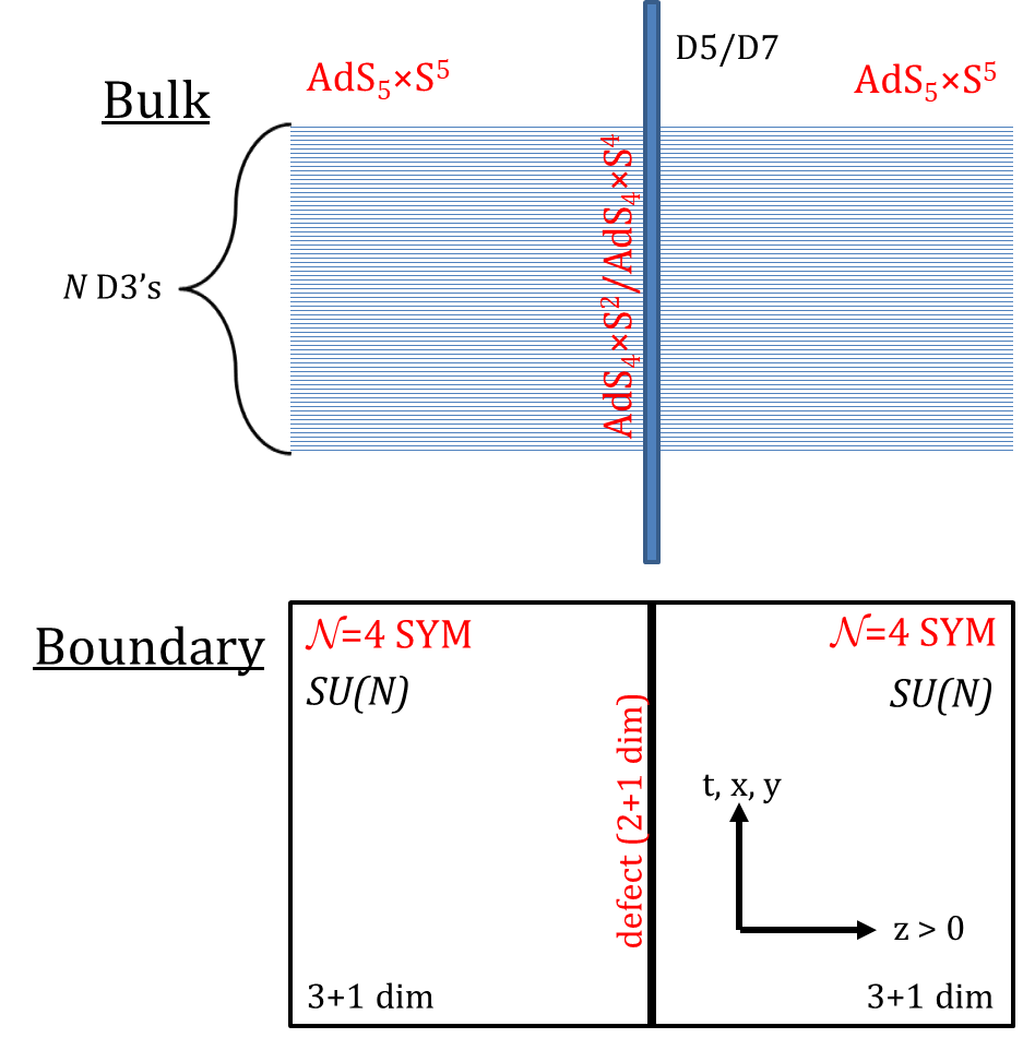
The insertion of the probe D5/D7-brane on the string theory side of the AdS/CFT correspondence (2) modifies it as follows (see figure 1, left). The bulk is still described by IIB string theory on AdS which is now bisected by a probe D5/D7-brane with worldvolume geometry AdS (probe D5-brane) or AdS (probe D7-brane). The dual field theory becomes a defect CFT that consists of two interacting parts. An SCFT4 ( SYM), coupled to a CFT that lives on a flat dimensional defect [17, 18]:
Due to the presence of the defect, the total bosonic symmetry of the system is reduced from to in the case of the probe D5-brane and in the case of the probe D7-brane. In the former case (probe D5-brane) the corresponding supersymmetry is halved, i.e. the 32-supercharge superconformal algebra of SYM becomes which has 16 supercharges, while in the latter case (probe D7-brane) the supersymmetry is broken completely.
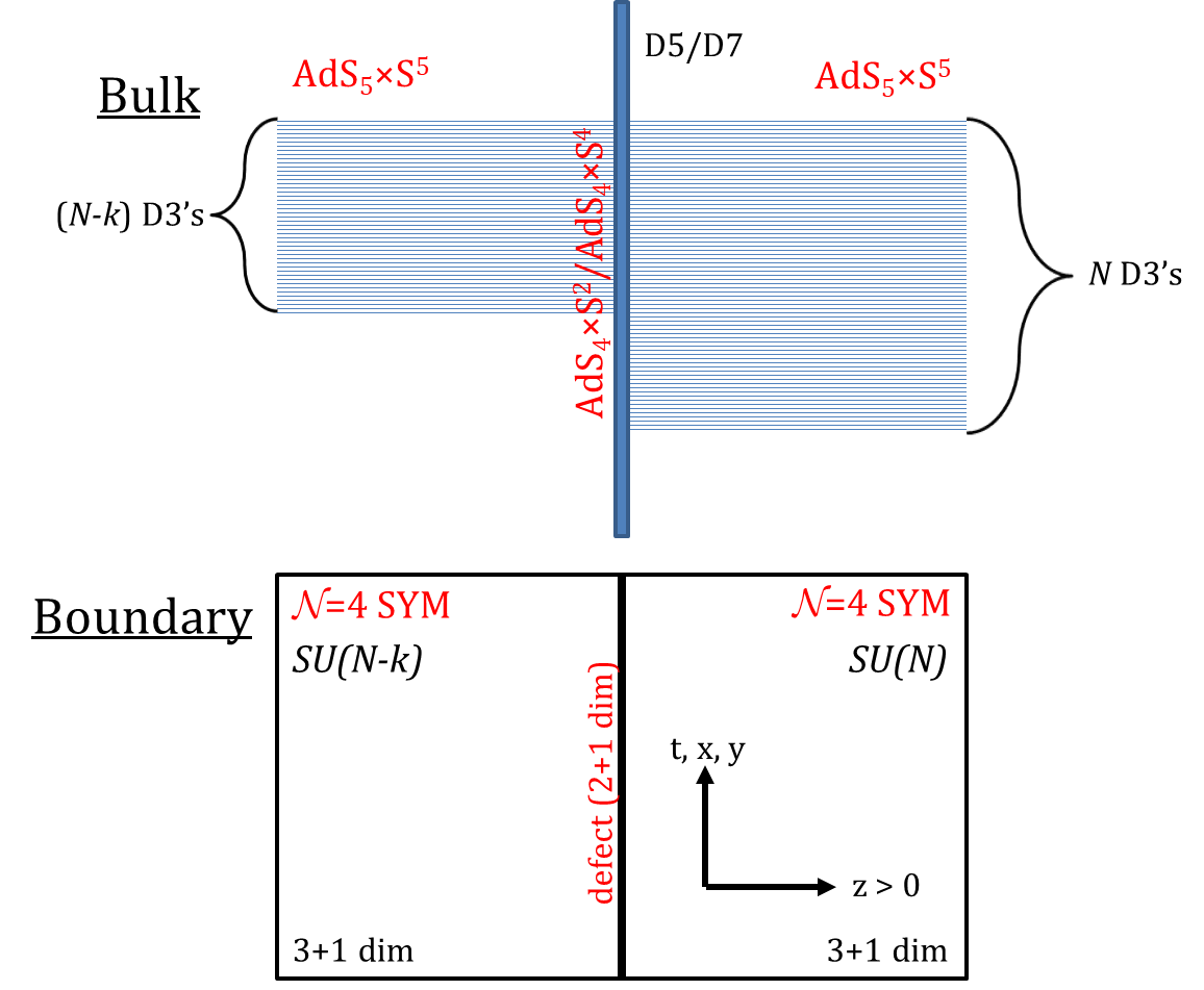
An interesting generalization of the D3-probe-D5 brane system (table 1) is obtained by supporting the worldvolume geometry of the probe D5-brane with units of magnetic flux through the S2 [14]. The D5-brane is again stable and wraps an AdS inside AdS. Its AdS coordinates satisfy
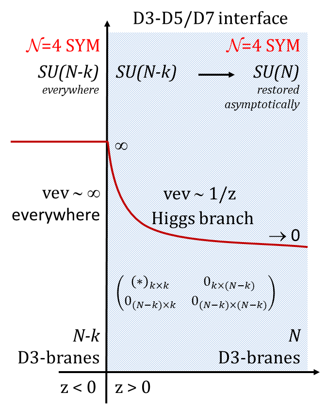
where is the ’t Hooft coupling. The flux forces exactly of the D3-branes () to terminate on the D5-brane (see figure 1, right). On the dual SCFT side the gauge group is different on each side of the defect, as gets broken to . Equivalently, the fields of SYM develop nonzero vevs. Note that the zero-flux case is smoothly recovered in the limit.
Both probe-brane geometries of the D3-D7 system (table 2) are unstable. For example, the S4 component of the D7-brane that is wrapped around the equator of S5 slips off towards either side of the equator after a small perturbation. One possible way to stabilize this system is by adding a homogeneous instanton on S4 with an instanton number given by [19]
The instanton is obtained from the BPST solution by replacing the 2-dimensional irreducible representation of by an dimensional one [20]. The flux again forces exactly of the D3-branes to end on the D7-brane (figure 1, right) and the gauge group of the dual gauge theory breaks from to . The D7-brane is stabilized when
We note that there exist more ways to stabilize the D3-D7 system of intersecting branes (oriented as in table 2). One comes about when the D7-brane is embedded in the full D3-brane geometry (22) instead of AdS (2.1) in the near-horizon limit [16]. Another way to lift the violation of the BF bound is by imposing an AdS cut-off [21, 22]. For the stabilization of the AdS geometry see the paper [23].
3 One-point functions
Once the rudiments of the AdS/dCFT correspondence have been laid down for the D3-probe-D5 and the D3-probe-D7 brane systems (brane orientation in tables 1–2), we need to set up a framework that will allow us to perform calculations on the defect CFT side. For this purpose we introduce the notion of the interface. Generally, an interface can be thought of as a (domain) wall that separates two different QFTs or even two copies of the same QFT. Interfaces are described by means of classical solutions of the QFT equations of motion that are known as ”fuzzy-funnel” solutions [24, 20].
In the present case of the dCFTs that are dual to the D3-probe-D5 and the D3-probe-D7 brane system (tables 1–2), we need an interface that separates the two copies of SYM with gauge groups (left) and (right) that lie on each side of the dimensional defect (see figure 2). To be a valid description, the corresponding fuzzy funnel solution must preserve the global symmetry of the dCFT, i.e. and its bosonic subgroup in the D3-D5 case and in the D3-D7 case.
For no vector and fermion fields, we want a solution of the equations of motion for the six real scalar fields of SYM ():
A manifestly symmetric solution of (3) for , is [25, 26, 24]:
where the matrices furnish a -dimensional representation of ,
The fuzzy-funnel solution (3) that describes the D3-probe-D5 brane interface also satisfies the Nahm equations:
and therefore induces a set of boundary conditions for the scalars that preserves one-half of the original supersymmetry [27], as it should. The D3-probe-D7 brane interface is described by the following symmetric solution of (3) [20]:
where are the -dimensional fuzzy S4 matrices [28, 20] and is the instanton number (2.3). The commutators of the -matrices furnish a -dimensional (anti-hermitian) irreducible representation of ,
3.1 Overlaps of matrix product states
As it has already been explained in §1.2, the insertion of a plane codimension-1 boundary in the bulk of a -dimensional CFT fixes the form of one-point functions of local scalar operators. Only the one-point functions of quasi-primary scalars are non-zero in the bulk and are given by (1.2):
where is the scaling dimension of the operator and its one-point function structure constant. Following Nagasaki and Yamaguchi [29], the tree-level one-point functions of single-trace scalar operators of a dCFT can be calculated in the planar limit () from the corresponding fuzzy-funnel solution. E.g. for the dCFT that is dual to the D3-probe-D5 brane system,
and similarly for the dCFT that is dual to the D3-probe-D7 brane system. Generally, is an symmetric tensor, invariant under cyclic permutations. The one-point function structure constant of (3.1) is then given by
where is the overlap of the matrix product state (MPS) with the state . For the two cases of interest (3), (3)
where the index refers to the auxiliary space of the color indices of the matrices and on which the trace operation applies. At tree-level, (3.1) implies
The overall normalization factor of the structure constant (3.1) originates from the normalization of single-trace operators as , which ensures that their two-point functions (1.1) will be normalized to unity:
within SYM, i.e. without the defect [30].
Chiral primary operators
The one-point functions of the chiral primary operators (CPOs)
where are symmetric traceless tensors that are associated to the S5 spherical harmonics,
have been calculated at tree-level for the matrix product states (3.1), in the planar limit [29, 31]. In the D3-D5 case [29], the spherical harmonics (3.1) are invariant under the global symmetry of the interface (3), so that the coordinates are given by (2.2)–(2.2):
and correspond to the metric (2.2). For small values of the ’t Hooft coupling constant (weak coupling), the one-point functions read
The one-point functions of the CPO’s (3.1) can also be computed at strong coupling () for the D3-D5 system (table 1). The supergravity calculation gives
To lowest-order in , (3.1) agrees with the weak-coupling result (3.1) in the double-scaling limit , const.
For the D3-D7 interface (3), the computation of the tree-level one-point functions of the CPOs (3.1) is similar [31]. If is the spherical harmonic (), then
gives the tree-level one-point functions of (3.1) for the D3-D7 MPS. At strong coupling (),
which again agrees with the weak-coupling result (3.1) in the limit , const.
Highest-weight states
Single-trace scalar operators like (3.1) have definite scaling dimensions and so they are eigenstates of a dilatation operator. To lowest order in , this dilatation operator coincides with the integrable closed (i.e. with periodic boundary conditions) spin chain:
that describes the mixing of single-trace scalar operators up to one loop in SYM [32]. The identity, permutation and trace operators that appear in (3.1) are respectively given by:
In what follows, we will only consider the 1-point functions of bulk operators that correspond to highest-weight eigenstates of the periodic spin chain (3.1), i.e. the ’s in (3.1) are constructed with the Bethe ansatz. For a study of 1-point functions of D3-D5 descendant operators, see [33].
3.2 Coordinate Bethe ansatz
The eigenstates of the spin chain (3.1) are constructed by means of the coordinate nested Bethe ansatz (cNBA).444For pedagogical introductions to the nested coordinate Bethe ansatz, the reader is referred to the theses [34, 35]. Nested Bethe states have the form:
where are three sets of rapidities for the spin chain excitations at positions ,
and are the momenta of the level-1 excitations ().
Nesting kets
The three sets or levels of spin chain excitations in (3.2) are associated with the nodes of the Dynkin diagram:
The nesting procedure for an spin chain of length , involves exciting the middle (momentum-carrying) node of the Dynkin diagram by inserting (level-1) excitations at the positions of the spin chain. Then the other two nodes of the Dynkin diagram are excited by placing (level-2) and (level-3) excitations at the positions and of the reduced chain (i.e. the spin chain that is formed by the level-1 excitations) respectively. We are led to the following nesting ket:
where
The total weight of the representation is
where are the corresponding Cartan charges. In (3.2), is the highest weight of and , , its simple roots so that the Cartan matrix is given by:
where the indices run from 1 to 3. The Dynkin indices of the representation (3.2) are
The next step is to replace each nesting ket that shows up in (3.2) by a single-trace scalar operator like (3.1). To this end, the spin chain excitations of the nesting kets (3.2) must be mapped to the scalar fields of the dCFT. It is customary to combine the six real scalar fields () into three complex scalars as follows:
Now the field content of the representation (3.2) is determined from the following associations:
where obviously the complex scalar field corresponds to the vacuum state of the spin chain, the field to the excitations of level-1 , to level-2, while the excitations of the third level are the three anti-holomorphic fields , , .
Nested Bethe wavefunction
The other basic ingredient of the Bethe eigenstates in (3.2) is the nested Bethe wavefunction . Omitting certain subtleties concerning the contribution of the anti-holomorphic excitations and ,555Details can be found in appendix E.5 of [36]. the wavefunction is given by:
where is the rapidity of the level- excitation at and denotes the permutations of the set for . The coefficients are determined from the following formula,
where and is the S-matrix for the Dynkin node ,
Bethe roots
The Bethe wavefunction must be periodic at each nesting level. Imposing its invariance under shifts of leads to the following set of Bethe equations:
which are satisfied by the rapidities of the excitations or Bethe roots. The cyclicity of the trace in single-trace operators such as (3.1) also implies that the total momentum of level-1 excitations (or momentum-carrying Bethe roots) is always zero:
It can be proven that the Bethe states constructed via (3.2) and mapped to a single-trace operator via (3.2)–(3.2), are indeed eigenstates of the spin chain (3.1) if the rapidities solve the Bethe equations (3.2)–(3.2) and obey (3.2). The corresponding eigenvalues/operator scaling dimensions are given by:
The Bethe wavefunction in (3.2)–(3.2) simplifies significantly if one instead of the full sector which includes all the fields (3.2)–(3.2), considers its two subsectors and .
The sector
The subsector contains only the two holomorphic scalars and . The trace operator (3.1) acts only on anti-holomorphic fields and so it does not contribute to the mixing matrix (3.1) which reduces to the Hamiltonian of the Heisenberg XXX1/2 spin chain:
The Bethe eigenstate becomes:
where denotes the number of magnons and
The vacuum state and the raising and lowering operators have been defined as
while the matrix and the normalization constant are given by:
where we have omitted the level subscripts from the Bethe roots. is not present in (3.2)–(3.2); it has been chosen in such a way that the coefficient of the term in (3.2) is equal to one.
The sector
The subsector contains the three holomorphic fields , and . Once more the trace operator does not contribute and the mixing matrix is the Heisenberg Hamiltonian (3.2). The wavefunction in (3.2) takes the following form:
where and give the total number of level-1 and level-2 excitations of the spin chain. In (3.2) we have also set and .
4 Solving the D3-D5 defect
All the necessary tools are now available for the computation of the tree-level one-point function structure constants (3.1), (3.1) for highest-weight eigenstates (Bethe states) of the spin chain (3.1) and the matrix product states (3.1), in the planar limit (). For the dCFT that is dual to the D3-probe-D5 brane system, the form of the corresponding interface (3) implies that the three holomorphic fields () are identical to the anti-holomorphic ones ().
4.1 One-point functions in the sector
The overlap of the D3-D5 matrix product state in (3.1) with an -magnon Bethe state (3.2) is the basic ingredient of the one-point function structure constant (3.1). It is given by
where is a permutation of letters and are the magnon momenta.
Selection rules
There exists a number of nifty selection rules for one-point functions in the sector [37]. In particular, has been found to vanish for all values of the bond dimension unless:
-
•
The length of the operator and the number of magnons/excitations is even.
-
•
The magnon total momentum is zero, .
-
•
The Bethe roots are fully balanced: .
The first of the above properties is proven by means of certain similarity transformations that furnish an automorphism of the algebra, while the second follows from trace cyclicity. The third selection rule is a consequence of the fact that the third conserved charge in the integrable hierarchy of conserved mutually commuting charges of the spin chain (3.2) annihilates the matrix product state, i.e. . More about this property will be said in §7 below. Fully balanced Bethe roots always appear in equal and opposite pairs.
Vacuum overlap
The vacuum overlap and one-point function () has the following form for any value of the bond dimension [37]:
where is the Hurwitz zeta function. The vacuum overlap is nonzero only when the length of the operator is even, in full accordance with the above selection rules.
Determinant formula
4.2 One-point functions in the sector
As we have explained, the sector contains the three holomorphic fields (3.2) of the theory. The Bethe eigenstates are constructed with the nested Bethe ansatz (3.2), (3.2) so that there are two types of excitations (, ) and two levels of Bethe roots, u and v. Let us first define the Baxter functions and :
The one-point functions in the sector (modulo ) are given by [39]:
As before these are only nonzero when the Bethe roots are fully balanced; also, and . The full set of selection rules can be found below. For the definitions of the matrices see (4.3)–(4.3). Also,
The validity of (4.2) has been checked numerically for a plethora of states that were obtained from the cNBA (3.2), (3.2). For , (4.2) reduces to the determinant formula of [40]. In the absence of excitations (), the determinant formula (4.1) is retrieved. A recent attempt to prove (4.2) using the representation theory of twisted Yangians can be found in [41].
4.3 One-point functions in the sector
The sector contains all the holomorphic and anti-holomorphic fields (3.2)-(3.2). There are three types of excitations and three sets of Bethe roots which must be fully balanced for the one-point function to be nonzero. Writing () and the 1-point functions in the sector are given, for all values of the bond dimension , by [39]:
where again we have omitted the overall factor . The definition of the Baxter functions and has been given in (4.2). The matrices and are defined as [42]:666There is a subtlety in the following formula, namely must be multiplied with whenever .
where is the Cartan matrix and the highest-weight of defined in (3.2). The indices of in (4.3)–(4.3) run from 1 to while those of run from 1 to . (4.3)–(4.3) equally apply to the and algebras, reducing to (4.1) in the former case. An equivalent definition of the norm matrices is given in appendix A. The prefactor in (4.3) can be related to the transfer matrix of the spin chain. More will be said in §6 below. Explicitly,
The determinant formula (4.3) has been verified numerically for a large number of states that were constructed from the cNBA (3.2), (3.2)–(3.2). The and formulas (4.1) and (4.2) are trivially recovered when the corresponding excitations are absent ( or ).
Selection rules
Once more, the one-point functions in the sector have been found to vanish for all values of the bond dimension unless:
-
•
The quantities or are both even.
-
•
The magnon total momentum is zero, .
-
•
All the levels of Bethe roots are fully balanced, i.e. they show up in equal and opposite pairs when the corresponding number of roots (, ) is even and the extra unpaired root vanishes, when the corresponding wing root number () is odd:
The selection rules trivially reduce to the ones when . They are also fully valid in the sector, i.e. when .
5 Solving the D3-D7 defect
The dCFT that is dual to the D3-probe-D7 brane system is an example of a non-supersymmetric defect for which a determinant formula for all its scalar tree-level one-point functions of Bethe states has been found. This dCFT is drastically different from the supersymmetric D3-D5 dCFT that we examined in the previous section. Not only the closed-form expression for its one-point functions is more involved, but also the corresponding selection rules and the overall structure of its scalar subsectors are different.
The D3-D7 interface is described by the MPS in (3.1) which is parameterized in terms of the -matrices. The corresponding bond dimension in (2.3) is a function of the parameter . As before, we also set , and for the excitation mode numbers.
Vacuum overlap
Selection rules
As it turns out, the overlaps of all the highest-weight eigenstates vanish unless the number of holomorphic excitations and in is respectively equal to the number of the anti-holomorphic fields and . (3.2)–(3.2) then directly imply that one-point functions vanish for all values of the parameter in the and subsectors and only the vacuum state and the sector can be nontrivial.
Moreover, the one-point functions have been found to vanish for all the values of the parameter unless:
-
•
The excitation mode numbers satisfy and is even.
-
•
The magnon total momentum is zero, .
- •
-
•
is odd and the wing rapidities are not identical, .
Determinant formula
Using the Baxter functions and that have been defined in (4.2), setting and also , , for the balanced Bethe roots, we find the following expression for one-point functions in the sector [41]:
omitting as usual the factor . The definition of the matrices has been given above in (4.3)–(4.3). See also (A). The prefactor is given by
however this expression is valid only for even values of . When is odd, one auxiliary Bethe root vanishes at each level and a indeterminate form arises. In this case becomes
where are given by
The determinant formulas (5)–(5) have been checked numerically for many states constructed by means of the nested Bethe ansatz (3.2), (3.2)–(3.2). For (5)–(5) trivially reduce to the corresponding formula of [43].
Here are some interesting special cases in which the formulae (5)–(5) simplify. For , (5) reads
whereas for , (5)–(5) take the following form
The prefactors that show up in the one-point function determinant formulas (4.3), (5) can again be related to the eigenvalues of the transfer matrix of the spin chain. We briefly explore this connection in the next section.
6 Fusion hierarchies
Every irreducible representation of that is parameterized by a semistandard Young tableau777Semistandard means that the entries of the YT increase weakly along each row and strictly along each column. with rows and columns gives rise to a transfer matrix (TM) of the spin chain. It can be shown that the eigenvalue of this TM satisfies the Hirota equation or T-system:
a difference equation that describes the fusion of transfer matrices ( is known as the spectral parameter). An equivalent representation of (6) can be obtained by the transformation
which leads to the so-called Y-system:
Nothing much changes in the above for spin chains obeying periodic or open boundary conditions (and the TM is single-row or double-row respectively). The T-system (6) affords a solution that can be expressed by the following tableau sum formula [44]
where the indices and correspond to the rows and the columns of the semistandard Young tableau that parameterize the irreducible representation of . The prefactors in (4.3), (5) are related to the transfer matrices. For the tableau sum formula (6) becomes
where the sum runs over all the semistandard Young tableaux of size .
6.1 D3-D5 system
6.2 D3-D7 system
7 Integrable defects
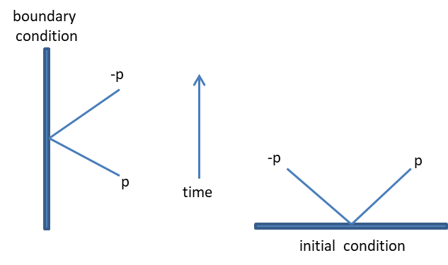
There is an interesting argument that allows to view defects as quantum quenches and vice-versa. According to Ghoshal and Zamolodchikov [45], there are two equivalent ways to describe an (integrable) QFT in the presence of a boundary/defect, one in which the defect operates as a wall or boundary condition which scatters off particles, and another (in the Wick-rotated frame of the first) where the defect operates as an initial condition for the pair-creation/annihilation of particles (see figure 3 below).
Quantum quenches
To further illustrate this point, let us first explain the notion of (global) quantum quench. Consider an isolated quantum many-particle system that is described in terms of a translationally-invariant, time-independent Hamiltonian with short-range interactions ( is a tunable parameter of the Hamiltonian, e.g. a coupling constant). At time the system is prepared to the ground state of . Then suddenly at the parameter is ”quenched” (i.e. changed) to a new value without affecting the initial state (”sudden approximation”). For the system evolves unitarily according to the Schrödinger equation
and may or may not equilibrate to a stationary state as . The restriction to short-range interactions (e.g. spin chains) is important given that systems with infinitely-ranged interactions have a different equilibration behavior. On the other hand there exist more quench protocols, e.g. when the initial state is not pure, or when translation invariance is limited to only a few sites of the system. The study of quantum quenches has exploded in recent years with a series of fascinating experiments involving ultra-cold trapped atoms (see e.g. [46] and references therein).
The evolution of the quenched system from small to large time scales is best studied through the time-dependent expectation values of various operators. These can often be related to overlaps of matrix product states and spin chain eigenstates like the ones we computed in the previous sections. To see this let us write the initial state in (7) as a matrix product state . The initial states are prepared as ground states of some Hamiltonian that is afterwards quenched to a periodic spin chain like (3.1), (3.2). The quenched Hamiltonian can be diagonalized as
while the evolution equation (7) takes the form
The post-quench expectation values of generic physical operators then become
where is the overlap of the initial state with the eigenstates of the quenched Hamiltonian .
Now it is known that in the absence of other conserved quantities, isolated Hamiltonian systems always relax to a thermal equilibrium, i.e. they thermalize. The stationary state is described by the Gibbs ensemble. In the presence of more conserved quantities, systems are known to relax to a generalized Gibbs ensemble (GGE). Integrable models demonstrate an unusual equilibration dynamics: they do not thermalize.888More about this interesting topic can be found in the collection of articles [47].
Considerable effort has therefore been devoted to the study of relaxation dynamics of integrable models. In order to overcome a number of difficulties that arise when applying the GGE, [48] proposed the study of quenches that arise from certain initial states that have been dubbed integrable initial states.
Note on integrability
Before proceeding to the definition of an integrable quench, let us briefly revisit the concept of integrability. Intuitively, integrability implies exact solvability. This follows from Liouville’s theorem which states that the equations of motion of a Hamiltonian system having degrees of freedom and an equal number of Poisson-commuting conserved quantities
is solvable by quadratures; is the total momentum, the Hamiltonian of the system and the Poisson bracket. In other words the solution can in principle be obtained by solving a finite number of algebraic equations and performing a finite number of integrations. Practically, there are very few integrable systems for which closed-form solutions can be found though.
The direct generalization of (7) to quantum systems seems to be (1):
i.e. the classical charges are promoted to operators and Poisson brackets to commutators. This definition however turns out to be neither sufficiently rigorous nor practical. Other definitions such as (2) solvability by the Bethe ansatz (diagonalizability), (3) multi-particle scattering that is factorizable in two-particle scatterings (non-diffractive scattering), etc. are also not completely consistent as sufficient conditions, despite being for the most part accurate as necessary conditions for quantum integrability. To day there is no general consensus as to the proper rigorous necessary and sufficient conditions of quantum integrability.
Integrable quenches
To formulate the definition of an integrable quench we consider an integrable Hamiltonian system with infinitely many mutually commuting conserved local charges
These charges can always be chosen to have a definite parity with respect to space reflections, i.e.
so that they can be divided into two classes according to their space parity, the even charges and the odd charges . In (7), stands for the space parity operator
An initial state that is represented by a matrix product state is integrable if it is annihilated by all the parity-odd conserved charges of the integrable hierarchy (7) [48]:
In fact there is a stronger version of (7) that involves the transfer matrix of the system:
The definitions (7)–(7) of integrable quenches have a number of immediate consequences for the form of matrix product state overlaps with the (Bethe) eigenstates of the Hamiltonian . For one, the overlaps vanish unless the rapidities of the excitations (Bethe roots) come in pairs of opposite signs as e.g. in (• ‣ 4.3)–(• ‣ 4.3). Moreover, the overlaps can be described by closed-form expressions (as e.g. in (4.3), (5)) with simple factorized descriptions.
Integrable defects
We can now go full circle by formulating the lattice version of the Ghoshal-Zamolodchikov rotation that was presented at the beginning of the section (see figure 3). Following [48] the initial states of closed spin chains are mapped to boundary states of open spin chains. The latter are determined in terms of a reflection matrix which provides the absorption amplitude of particle pairs scattering off the boundary. Integrable quenches satisfying (7)–(7) correspond to integrable boundaries whose reflection matrices satisfy the boundary Yang-Baxter (or reflection) equation [48, 49, 50, 51].
The integrable boundary state/reflection matrix controls the set of integrable boundary conditions that are obeyed by the open spin chains. Besides single-trace operators that are composed exclusively of bulk scalars , defect CFTs with boundary degrees of freedom like (2.3), also have operators that contain defect fields, e.g. , where is a defect scalar. The set of integrable spin chains with open boundary conditions that give the corresponding one-loop dilatation operator of the D3-D5 interface has been studied in [52, 53].
Here is a summary of the main properties of integrable quenches/defects:
-
•
The parity-odd conserved charges annihilate the MPS, (7).
-
•
The transfer matrix obeys (7).
-
•
Boundary states corresponding to open spin chain boundary conditions are integrable.
-
•
Bethe roots are fully balanced, i.e. they appear in pairs of opposite signs.
-
•
Closed-form expressions are possible for overlaps of Bethe eigenstates with MPSs.
It has been proven in [39] that the matrix product states (3.1) that are relevant to the D3-D5 and the D3-D7 interfaces are integrable, namely they satisfy the criteria (7)–(7). Both interfaces afford closed-form expressions for all the tree-level one-point functions of their bulk single-trace scalar operators that are highest-weight states of the corresponding dilatation operators, cf. (4.3), (5). The other main consequence of integrability, the pairing of Bethe roots (• ‣ 4.3)–(• ‣ 4.3), has also been checked for a large number of nontrivial operators for both interfaces in (3.1).
8 Summary and outlook
Following the recent works [39, 41], we have presented closed-form expressions (4.3), (5) for all the tree-level one-point functions of the defect CFTs that are dual to the symmetric D3-probe-D5 brane system with units of magnetic flux and the symmetric D3-probe-D7 brane system with units of instanton flux. Working in the planar limit () and at weak ’t Hooft coupling (), we concentrated on bulk single-trace scalar operators that are highest-weight (Bethe) states of the integrable spin chain (3.1).
Checking the validity of the determinant formulas (4.2), (4.3), (5) and the corresponding selection rules involves solving the Bethe equations (3.2)–(3.2). The Bethe roots are used both in numerically obtaining the one-point functions from the overlaps of the nested Bethe states (3.2), (3.2)–(3.2) and in computing their values from the aforementioned determinant formulas. For all the checks that are mentioned in the present talk we have used an algorithm (fast Bethe solver) that was developed in [54, 55, 56]. This program quickly solves the Bethe equations by demanding the solutions of the QQ-relation to be polynomials.
In order to come closer to solving the defects (in the sense explained in §1), more input is needed such as the data from the pure CFT ( SYM), the boundary and the bulk-boundary data. As we mentioned in §1.2 these data are not all independent; the boundary CFT bootstrap program aims to determine their precise relationship. This is certainly not the end of the story as there are more sectors in the theory and far more operators such as descendants and multiple-trace operators. Furthermore, integrability may be used to go beyond the tree-level approximation and the large- limit, as well as computing the values of more and more interesting observables.
Naturally, there are a lot of topics in this rapidly expanding field that we didn’t touch upon. Below we collect a list of references for further reading. One could also consult the excellent reviews [57, 58] as well as the theses [59, 60].
An important open question concerns the extension of the results herein presented to strong coupling. A preliminary computation from string theory has been carried out in [38], while one-loop corrections to the one-point functions of the supersymmetric D3-D5 system have been computed in [61, 62, 63] (see also the master’s thesis [64]) and in [65] for the non-supersymmetric D3-D7 system. Recently the paper [66] appeared together with an approach via supersymmetric localization [67, 68] (see also its precursors [69, 70]). Also quite recently the paper [42] set up the computation of one-point functions in sections that contain gluon and fermion fields. See also [71] for a study of the properties of spinning strings in the context of the AdS/dCFT correspondence.
For applications to Wilson loops and lines see [72, 73, 74, 75, 76, 77].999Note also the relation of Wilson loop calculations to holographic entanglement entropy (cf. [78]). The calculation of two-point functions and various applications to the conformal bootstrap program was taken up in [33, 79]. The non-supersymmetric non-integrable symmetric dCFT that is dual to the D3-probe-D7 system was examined at tree and one-loop order in [80, 81], while the beta-deformed D3-probe-D5 system is discussed in [82]. Many more holographic defect CFTs that are based on probe-brane systems and could possibly be studied by similar methods are known, see for example [83, 84, 85]. The S-dual of the D3-D5 system is the D3-NS5 brane system,101010The author is thankful to C. Bachas for an interesting discussion about this system. the integrability of which has been studied in [86]. An interesting future direction is the formulation of a defect version for the ABJM theory,111111The author thanks S. Penati for drawing his attention to this subject. see [87] for a relevant preliminary investigation.
The relation of matrix product states to the Néel state was first explored in [37] and soon after in [88]. More recently, the 3-point structure constants of certain determinant operators and a non-protected operator of SYM were expressed in terms of determinant formulas similar to the ones we have been presenting in this talk [89, 90, 91]. The structure constants are interpreted as -functions or boundary entropies which are measures of the boundary degrees of freedom in a QFT. The -function is obtained from the overlap of boundary states with the ground state of the system; see [92] for a study relative to the purposes of the present work.
The subject of boundary and defect CFTs (holographic or not) is currently at the focus of intense research activity, see e.g. the recent review [93] and the events [94, 95, 96, 97]. In terms of physical applications that are relevant to the present approach, we single out the proposal of the D3-D7 system as a holographic model of graphene [15] and topological insulators [98]. The connection with quantum quenches that was analyzed in §7 has sparked a fruitful exchange of ideas between the two communities, further references on this subject include [99, 100, 101, 102, 103].
9 Acknowledgements
The author is grateful to George Zoupanos and the organizers of the 2019 Corfu Summer Institute for the invitation to participate to the Conference on Recent Developments in Strings and Gravity. The author is thankful to M. Axenides, M. de Leeuw, E. Floratos, C. Kristjansen and K. Zarembo. Special thanks to M. Axenides for his feedback after reading various parts of the manuscript. The author would also like to thank H. B. Nielsen for illuminating discussions during the conference.
The author also thanks C. Papadopoulos and C. Markou for granting him access to the computing facilities of the Institute of Nuclear and Particle Physics at NCSR ”Demokritos” and J. Ambjørn for the access to his computer system at the Niels Bohr Institute .
The author’s research has received funding from the Hellenic Foundation for Research and Innovation (HFRI) and the General Secretariat for Research and Technology (GSRT), in the framework of the first post-doctoral researchers support, under grant agreement No. 2595.
Appendix A Norm of Bethe states
We define three functions as the logarithm of the Bethe equations (3.2)–(3.2):
where () and consider the following Jacobian, that is known as the norm matrix:
with
Supposing that the Bethe roots are paired as in (• ‣ 4.3)–(• ‣ 4.3) it can be shown that the norm matrix (A) takes the form
where the submatrices correspond to the norm matrices of the and subsectors, cf. [40]. It can be proven that the determinant of the norm matrix (A), (A) factorizes as follows
where (and so on for , , , , ) and
(A) agrees with the corresponding formulas in the and sectors, cf. [40]. We have checked the equivalence of the definition (4.3)–(4.3) with (A) for a large number of states. According to the thesis [35] the norm of the Bethe states (3.2), (3.2)–(3.2) is given by the formula:
which also has the factorization property as a consequence of (A).
References
- [1] A. M. Polyakov, Conformal symmetry of critical fluctuations, JETP Lett. 12 (1970) 381. [Pisma Zh. Eksp. Teor. Fiz. 12 (1970) 538].
- [2] A. S. Wightman, Quantum field theory in terms of vacuum expectation values, Phys. Rev. 101 (1956) 860.
- [3] S. Ferrara, A. F. Grillo, and R. Gatto, Tensor representations of conformal algebra and conformally covariant operator product expansion, Annals Phys. 76 (1973) 161.
- [4] A. M. Polyakov, Nonhamiltonian approach to conformal quantum field theory, Zh. Eksp. Teor. Fiz. 66 (1974) 23. [Sov. Phys. JETP, 39 (1974) 9].
- [5] J. L. Cardy, Conformal invariance and surface critical behavior, Nucl. Phys. B240 (1984) 514.
- [6] J. L. Cardy, Conformal invariance, in Phase transitions and critical phenomena (C. Domb and J. L. Lebowitz, eds.), vol. 11, p. 55, Academic press, London, 1987.
- [7] D. M. McAvity and H. Osborn, Conformal field theories near a boundary in general dimensions, Nucl. Phys. B455 (1995) 522, [cond-mat/9505127].
- [8] P. Liendo, L. Rastelli, and B. C. van Rees, The bootstrap program for boundary CFTd, JHEP 07 (2013) 113, [arXiv:1210.4258].
- [9] J. M. Maldacena, The large-N limit of superconformal field theories and supergravity, Adv. Theor. Math. Phys. 2 (1998) 231, [hep-th/9711200].
- [10] A. Karch and L. Randall, Localized gravity in string theory, Phys. Rev. Lett. 87 (2001) 061601, [hep-th/0105108].
- [11] O. Aharony, S. S. Gubser, J. Maldacena, H. Ooguri, and Y. Oz, Large-N field theories, string theory and gravity, Phys. Rep. 323 (2000) 183, [hep-th/9905111].
- [12] C. Kristjansen, M. Staudacher, and A. Tseytlin, Gauge-string duality and integrability: Progress and outlook, J. Phys. A42 (2009) 250301.
- [13] N. Beisert et al., Review of AdS/CFT integrability: An overview, Lett. Math. Phys. 99 (2012) 3, [arXiv:1012.3982].
- [14] A. Karch and L. Randall, Open and closed string interpretation of susy CFT’s on branes with boundaries, JHEP 06 (2001) 063, [hep-th/0105132].
- [15] S.-J. Rey, String theory on thin semiconductors: Holographic realization of Fermi points and surfaces, Prog. Theor. Phys. Suppl. 177 (2009) 128, [arXiv:0911.5295].
- [16] J. L. Davis, P. Kraus, and A. Shah, Gravity dual of a quantum Hall plateau transition, JHEP 11 (2008) 020, [arXiv:0809.1876].
- [17] O. DeWolfe, D. Freedman, and H. Ooguri, Holography and defect conformal field theories, Phys. Rev. D66 (2002) 025009, [hep-th/0111135].
- [18] J. Erdmenger, Z. Guralnik, and I. Kirsch, Four-dimensional superconformal theories with interacting boundaries or defects, Phys. Rev. D66 (2002) 025020, [hep-th/0203020].
- [19] R. C. Myers and M. C. Wapler, Transport properties of holographic defects, JHEP 12 (2008) 115, [arXiv:0811.0480].
- [20] N. R. Constable, R. C. Myers, and O. Tafjord, Non-abelian brane intersections, JHEP 06 (2001) 023, [hep-th/0102080].
- [21] D. Kutasov, J. Lin, and A. Parnachev, Conformal phase transitions at weak and strong coupling, Nucl. Phys. B858 (2012) 155, [arXiv:1107.2324].
- [22] A. Mezzalira and A. Parnachev, A holographic model of quantum Hall transition, Nucl. Phys. B904 (2016) 448, [arXiv:1512.06052].
- [23] O. Bergman, N. Jokela, G. Lifschytz, and M. Lippert, Quantum Hall effect in a holographic model, JHEP 10 (2010) 063, [arXiv:1003.4965].
- [24] N. R. Constable, R. C. Myers, and O. Tafjord, The noncommutative bion core, Phys. Rev. D61 (2000) 106009, [hep-th/9911136].
- [25] D.-E. Diaconescu, D-branes, monopoles and Nahm equations, Nucl. Phys. B503 (1997) 220, [hep-th/9608163].
- [26] A. Giveon and D. Kutasov, Brane dynamics and gauge theory, Rev. Mod. Phys. 71 (1999) 983, [hep-th/9802067].
- [27] D. Gaiotto and E. Witten, Supersymmetric boundary conditions in super Yang-Mills theory, J. Stat. Phys. 135 (2009) 789, [arXiv:0804.2902].
- [28] J. Castelino, S. Lee, and W. Taylor, Longitudinal 5-branes as 4-spheres in matrix theory, Nucl. Phys. B526 (1998) 334, [hep-th/9712105].
- [29] K. Nagasaki and S. Yamaguchi, Expectation values of chiral primary operators in holographic interface CFT, Phys. Rev. D86 (2012) 086004, [arXiv:1205.1674].
- [30] S. Lee, S. Minwalla, M. Rangamani, and N. Seiberg, Three point functions of chiral operators in , SYM at large , Adv. Theor. Math. Phys. 2 (1998) 697, [hep-th/9806074].
- [31] C. Kristjansen, G. W. Semenoff, and D. Young, Chiral primary one-point functions in the D3-D7 defect conformal field theory, JHEP 01 (2013) 117, [arXiv:1210.7015].
- [32] J. A. Minahan and K. Zarembo, The Bethe ansatz for super Yang-Mills, JHEP 03 (2003) 013, [hep-th/0212208].
- [33] M. de Leeuw, A. C. Ipsen, C. Kristjansen, K. E. Vardinghus, and M. Wilhelm, Two-point functions in AdS/dCFT and the boundary conformal bootstrap equations, JHEP 08 (2017) 020, [arXiv:1705.03898].
- [34] K. Okamura, Aspects of integrability in AdS/CFT duality. PhD thesis, Tokyo U., 2007. arXiv:0803.3999.
- [35] J. Escobedo, Integrability in AdS/CFT: Exact results for correlation functions. PhD thesis, Waterloo U., 2012.
- [36] B. Basso, F. Coronado, S. Komatsu, H. Lam, P. Vieira, and D. Zhong, Asymptotic four point functions, JHEP 07 (2019) 082, [arXiv:1701.04462].
- [37] M. de Leeuw, C. Kristjansen, and K. Zarembo, One-point functions in defect CFT and integrability, JHEP 08 (2015) 098, [arXiv:1506.06958].
- [38] I. Buhl-Mortensen, M. de Leeuw, C. Kristjansen, and K. Zarembo, One-point functions in AdS/dCFT from matrix product states, JHEP 02 (2016) 052, [arXiv:1512.02532].
- [39] M. de Leeuw, C. Kristjansen, and G. Linardopoulos, Scalar one-point functions and matrix product states of AdS/dCFT, Phys. Lett. B781 (2018) 238, [arXiv:1802.01598].
- [40] M. de Leeuw, C. Kristjansen, and S. Mori, AdS/dCFT one-point functions of the sector, Phys. Lett. B763 (2016) 197, [arXiv:1607.03123].
- [41] M. de Leeuw, T. Gombor, C. Kristjansen, G. Linardopoulos, and B. Pozsgay, Spin chain overlaps and the twisted Yangian, JHEP 01 (2020) 176, [arXiv:1912.09338].
- [42] C. Kristjansen, D. Müller, and K. Zarembo, Integrable boundary states in D3-D5 dCFT: beyond scalars, arXiv:2005.01392.
- [43] M. de Leeuw, C. Kristjansen, and G. Linardopoulos, One-point functions of non-protected operators in the symmetric D3-D7 dCFT, J. Phys. A50 (2017) 254001, [arXiv:1612.06236].
- [44] A. Kuniba, T. Nakanishi, and J. Suzuki, T-systems and Y-systems in integrable systems, J. Phys. A44 (2011) 103001, [arXiv:1010.1344].
- [45] S. Ghoshal and A. B. Zamolodchikov, Boundary S-matrix and boundary state in two-dimensional integrable quantum field theory, Int. J. Mod. Phys. A9 (1994) 3841, [hep-th/9306002]. [Erratum: Int. J. Mod. Phys. A9 (1994) 4353].
- [46] T. Langen, T. Gasenzer, and J. Schmiedmayer, Prethermalization and universal dynamics in near-integrable quantum systems, J. Stat. Mech. 1606 (2016) 064009, [arXiv:1603.09385].
- [47] P. Calabrese, F. H. L. Essler, G. Mussardo, et al., Introduction to quantum integrability in out of equilibrium systems, J. Stat. Mech. (2016) 064001–064011.
- [48] L. Piroli, B. Pozsgay, and E. Vernier, What is an integrable quench?, Nucl. Phys. B925 (2017) 362, [arXiv:1709.04796].
- [49] L. Piroli, E. Vernier, P. Calabrese, and B. Pozsgay, Integrable quenches in nested spin chains I: The exact steady states, J. Stat. Mech. 1906 (2019) 063103, [arXiv:1811.00432].
- [50] L. Piroli, E. Vernier, P. Calabrese, and B. Pozsgay, Integrable quenches in nested spin chains II: Fusion of boundary transfer matrices, J. Stat. Mech. 1906 (2019) 063104, [arXiv:1812.05330].
- [51] B. Pozsgay, L. Piroli, and E. Vernier, Integrable matrix product states from boundary integrability, SciPost Phys. 6 (2019) 062, [arXiv:1812.11094].
- [52] O. DeWolfe and N. Mann, Integrable open spin chains in defect conformal field theory, JHEP 04 (2004) 035, [hep-th/0401041].
- [53] A. C. Ipsen and K. E. Vardinghus, The dilatation operator for defect conformal SYM, arXiv:1909.12181.
- [54] C. Marboe and D. Volin, Quantum spectral curve as a tool for a perturbative quantum field theory, Nucl. Phys. B899 (2015) 810, [arXiv:1411.4758].
- [55] C. Marboe and D. Volin, The full spectrum of AdS5/CFT4 I: Representation theory and one-loop Q-system, J. Phys. A51 (2018) 165401, [arXiv:1701.03704].
- [56] C. Marboe, The AdS/CFT spectrum via integrability-based algorithms. PhD thesis, Trinity College Dublin, 2017.
- [57] M. de Leeuw, A. C. Ipsen, C. Kristjansen, and M. Wilhelm, Introduction to integrability and one-point functions in SYM and its defect cousin, Les Houches Lect. Notes 106 (2019) [arXiv:1708.02525].
- [58] M. de Leeuw, One-point functions in AdS/dCFT, J. Phys. A (2019) to appear, [arXiv:1908.03444].
- [59] E. Widen, Exact results in supersymmetric field theories: A dissertation on the defect and deformed. PhD thesis, Uppsala U., 2019.
- [60] K. E. Vardinghus, Boundaries of integrability in AdS/dCFT. PhD thesis, Copenhagen U., 2019.
- [61] I. Buhl-Mortensen, M. de Leeuw, A. C. Ipsen, C. Kristjansen, and M. Wilhelm, One-loop one-point functions in gauge-gravity dualities with defects, Phys. Rev. Lett. 117 (2016) 231603, [arXiv:1606.01886].
- [62] I. Buhl-Mortensen, M. de Leeuw, A. C. Ipsen, C. Kristjansen, and M. Wilhelm, A quantum check of AdS/dCFT, JHEP 01 (2017) 098, [arXiv:1611.04603].
- [63] I. Buhl-Mortensen, M. de Leeuw, A. Ipsen, C. Kristjansen, and M. Wilhelm, Asymptotic one-point functions in gauge-string duality with defects, Phys. Rev. Lett. 119 (2017) 261604, [arXiv:1704.07386].
- [64] B. Guo, Lollipop diagrams in defect super Yang-Mills theory, Master’s thesis, British Columbia U., 2017.
- [65] A. Gimenez-Grau, C. Kristjansen, M. Volk, and M. Wilhelm, A quantum framework for AdS/dCFT through fuzzy spherical harmonics on S4, JHEP 04 (2020) 132, [arXiv:1912.02468].
- [66] T. Gombor and Z. Bajnok, Boundary states, overlaps, nesting and bootstrapping AdS/dCFT, arXiv:2004.11329.
- [67] Y. Wang, Taming defects in super Yang-Mills, arXiv:2003.11016.
- [68] S. Komatsu and Y. Wang, Non-perturbative defect one-point functions in planar super-Yang-Mills, arXiv:2004.09514.
- [69] B. Robinson and C. F. Uhlemann, Supersymmetric D3/D5 for massive defects on curved space, JHEP 12 (2017) 143, [arXiv:1709.08650].
- [70] B. Robinson, Supersymmetric localization and probe branes in the AdS/CFT correspondence. PhD thesis, Washington U., Seattle, 2017.
- [71] K. Okamura, Y. Takayama, and K. Yoshida, Open spinning strings and AdS/dCFT duality, JHEP 01 (2006) 112, [hep-th/0511139].
- [72] K. Nagasaki, H. Tanida, and S. Yamaguchi, Holographic interface-particle potential, JHEP 01 (2012) 139, [arXiv:1109.1927].
- [73] M. de Leeuw, A. C. Ipsen, C. Kristjansen, and M. Wilhelm, One-loop Wilson loops and the particle-interface potential in AdS/dCFT, Phys. Lett. B768 (2017) 192, [arXiv:1608.04754].
- [74] J. Aguilera-Damia, D. H. Correa, and V. I. Giraldo-Rivera, Circular Wilson loops in defect conformal field theory, JHEP 03 (2017) 023, [arXiv:1612.07991].
- [75] M. Preti, D. Trancanelli, and E. Vescovi, Quark-antiquark potential in defect conformal field theory, JHEP 10 (2017) 079, [arXiv:1708.04884].
- [76] S. Bonansea, S. Davoli, L. Griguolo, and D. Seminara, Circular Wilson loops in defect SYM: phase transitions, double-scaling limits and OPE expansions, JHEP 03 (2020) 084, [arXiv:1911.07792].
- [77] S. Bonansea, K. Idiab, C. Kristjansen, and M. Volk, Wilson lines in AdS/dCFT, arXiv:2004.01693.
- [78] D. Seminara, J. Sisti, and E. Tonni, Holographic entanglement entropy in AdS4/BCFT3 and the Willmore functional, JHEP 08 (2018) 164, [arXiv:1805.11551].
- [79] E. Widen, Two-point functions of -subsector and length-two operators in dCFT, Phys. Lett. B773 (2017) 435, [arXiv:1705.08679].
- [80] A. Gimenez-Grau, C. Kristjansen, M. Volk, and M. Wilhelm, A quantum check of non-supersymmetric AdS/dCFT, JHEP 01 (2019) 007, [arXiv:1810.11463].
- [81] M. de Leeuw, C. Kristjansen, and K. E. Vardinghus, A non-integrable quench from AdS/dCFT, Phys. Lett. B798 (2019) 134940, [arXiv:1906.10714].
- [82] E. Widen, One-point functions in -deformed SYM with defect, JHEP 11 (2018) 114, [arXiv:1804.09514].
- [83] N. R. Constable, J. Erdmenger, Z. Guralnik, and I. Kirsch, Intersecting D3-branes and holography, Phys. Rev. D68 (2003) 106007, [hep-th/0211222].
- [84] M. Ammon, J. Erdmenger, R. Meyer, A. O’Bannon, and T. Wrase, Adding flavor to AdS(4)/CFT(3), JHEP 11 (2009) 125, [arXiv:0909.3845].
- [85] J. Erdmenger, C. M. Melby-Thompson, and C. Northe, Holographic RG flows for Kondo-like impurities, arXiv:2001.04991.
- [86] M. Rapc̆ák, Nonintegrability of NS5-like interface in supersymmetric Yang-Mills, arXiv:1511.02243.
- [87] K. Sakai and S. Terashima, Integrability of BPS equations in ABJM theory, JHEP 11 (2013) 002, [arXiv:1308.3583].
- [88] O. Foda and K. Zarembo, Overlaps of partial Néel states and Bethe states, J. Stat. Mech. 1602 (2016) 023107, [arXiv:1512.02533].
- [89] Y. Jiang, S. Komatsu, and E. Vescovi, Structure constants in SYM at finite coupling as worldsheet -function, arXiv:1906.07733.
- [90] Y. Jiang, S. Komatsu, and E. Vescovi, Exact three-point functions of determinant operators in planar supersymmetric Yang-Mills theory, Phys. Rev. Lett. 123 (2019) 191601, [arXiv:1907.11242].
- [91] Y. Jiang and B. Pozsgay, On exact overlaps in integrable spin chains, arXiv:2002.12065.
- [92] I. Kostov, D. Serban, and D.-L. Vu, Boundary TBA, trees and loops, Nucl. Phys. B949 (2019) 114817, [arXiv:1809.05705].
- [93] N. Andrei et al., Boundary and defect CFT: Open problems and applications, 2018. arXiv:1810.05697.
- [94] Boundary and defect conformal field theory: Open problems and applications, workshop, Royal Society, Chicheley Hall, 7–8 September 2017.
- [95] Defects in topological and conformal field theory, workshop, King’s College London, 27–28 June 2019.
- [96] Boundaries and defects in quantum field theory, meeting, Perimeter Institute for Theoretical Physics, 6–9 August 2019.
- [97] Quantum field theory at the boundary, program, Mainz Institute for Theoretical Physics, Johannes Gutenberg University, 14 September–2 October 2020.
- [98] C. Kristjansen and G. W. Semenoff, The D3-probe-D7 brane holographic fractional topological insulator, JHEP 10 (2016) 079, [arXiv:1604.08548].
- [99] B. Bertini, E. Tartaglia, and P. Calabrese, Entanglement and diagonal entropies after a quench with no pair structure, J. Stat. Mech. 1806 (2018) 063104, [arXiv:1802.10589].
- [100] L. Piroli, Nonequilibrium quantum states of matter. PhD thesis, SISSA, 2018.
- [101] G. Perfetto, L. Piroli, and A. Gambassi, Quench action and large deviations: Work statistics in the one-dimensional Bose gas, Phys. Rev. E100 (2019) 032114, [arXiv:1904.06259].
- [102] R. Modak, L. Piroli, and P. Calabrese, Correlation and entanglement spreading in nested spin chains, J. Stat. Mech. 1909 (2019) 093106, [arXiv:1906.09238].
- [103] N. J. Robinson, A. J. J. M. de Klerk, and J.-S. Caux, On computing non-equilibrium dynamics following a quench, arXiv:1911.11101.