Leveraging large-deviation statistics to decipher the stochastic properties of measured trajectories

Abstract

Extensive time-series encoding the position of particles such as viruses, vesicles, or individual proteins are routinely garnered in single-particle tracking experiments or supercomputing studies. They contain vital clues on how viruses spread or drugs may be delivered in biological cells. Similar time-series are being recorded of stock values in financial markets and of climate data. Such time-series are most typically evaluated in terms of time-average mean-squared displacements, which remain random variables for finite measurement times. Their statistical properties are different for different physical stochastic processes, thus allowing us to extract valuable information on the stochastic process itself. To exploit the full potential of the statistical information encoded in measured time-series we here propose an easy-to-implement and computationally inexpensive new methodology, based on deviations of the time-averaged mean-squared displacement from its ensemble average counterpart. Specifically, we use the upper bound of these deviations for Brownian motion to check the applicability of this approach to simulated and real data sets. By comparing the probability of deviations for different data sets, we demonstrate how the theoretical bound for Brownian motion reveals additional information about observed stochastic processes. We apply the large-deviation method to data sets of tracer beads tracked in aqueous solution, tracer beads measured in mucin hydrogels, and of geographic surface temperature anomalies. Our analysis shows how the large-deviation properties can be efficiently used as a simple yet effective routine test to reject the Brownian motion hypothesis and unveil crucial information on statistical properties such as ergodicity breaking and short-time correlations.

I Introduction

Brownian Motion (BM) is characterized by the linear scaling with time of the mean squared displacement (MSD), $\langle\mathbf{r}^{2}(t)\rangle=2dDt$ in $d$ dimensions, where $D$ is the diffusion coefficient and angular brackets denote the ensemble average over a large number of particles. In many biological and soft-matter systems, this linear scaling has been reported to be violated hoff13 ; lenerev ; krapf11 ; tabei . Instead, anomalous diffusion with the power-law scaling $\langle\mathbf{r}^{2}(t)\rangle\simeq t^{\alpha}$ of the MSD is observed. The anomalous diffusion exponent $\alpha$ characterizes subdiffusion when $0<\alpha<1$ and superdiffusion when $\alpha>1$ metz12 ; igorsoft ; metz14 .

Passive and actively-driven diffusive motion are key to the spreading of viruses, vesicles, or proteins in living biological cells seisenhuber ; christine ; gratton . Pinpointing the precise details of their dynamics will ultimately pave the way for improved strategies in drug delivery, or lead to better understanding of molecular signaling used in gene silencing techniques. Similarly, improved analyses of the stochastic dynamics of financial or climate time series will allow us to find better comprehension of economic markets or climate impact.

The most-used observable in the analysis of time-series $\mathbf{r}(t)$ garnered for the position of viruses or vesicles by modern single-particle tracking setups in biological cells or for the key quantities in financial or climate dynamics, such as price or temperature, is the time-averaged MSD (TAMSD) metz12 ; metz14

$$\overline{\delta^{2}(\Delta)}=\frac{1}{T-\Delta}\int_{0}^{T-\Delta}\Big{[}\mathbf{r}(t+\Delta)-\mathbf{r}(t)\Big{]}^{2}dt,$$ (1)

expressed as function of the lag time $\Delta$. For BM at sufficiently long $T$, the TAMSD (1) converges to the MSD, formally $\lim_{T\to\infty}\overline{\delta^{2}(\Delta)}=\langle\mathbf{r}^{2}(\Delta)\rangle=2dD\Delta$, reflecting the ergodicity of this process in the Boltzmann-Khinchin sense stas . Anomalous diffusion processes may be MSD-ergodic, with a TAMSD of the form $\overline{\delta^{2}(\Delta)}\simeq\Delta^{\beta}$ with $\beta=\alpha$, e.g., fractional Brownian motion (FBM), or they may be "weakly non-ergodic", e.g., $\beta=1$ for continuous time random walks (CTRWs) with scale-free waiting times metz12 ; metz14 ; stas .

Due to the random nature of the process, the TAMSD is inherently irreproducible from one trajectory to another, even for BM. The emerging amplitude spread is quantified in terms of the dimensionless variable $\xi=\overline{\delta^{2}(\Delta)}/\left<\overline{\delta^{2}(\Delta)}\right>$, where $\left<\overline{\delta^{2}(\Delta)}\right>$ is the average of the TAMSD over many trajectories stas ; metz14 . The variance of $\xi$ is the ergodicity breaking parameter $\mathrm{EB}(\Delta)=\left<\xi^{2}\right>-1$. Together with the full distribution $\phi(\xi)$, EB provides valuable information on the underlying stochastic process metz14 . For BM, in the limit of large $T$, each realization leads to the same result, $\phi(\xi)=\delta(\xi-1)$ and $\mathrm{EB}=0$. For scale-free CTRWs, even in the limit $T\to\infty$ EB retains a finite value and the TAMSD remains a random variable, albeit with a known distribution $\phi(\xi)$ metz12 ; metz14 ; stas .

The MSD and TAMSD or, alternatively, the power spectrum and its single trajectory analog dieg18 ; dieg19 , are insufficient to fully characterize a measured stochastic process. A TAMSD of the form $\overline{\delta^{2}(\Delta)}\simeq\Delta$, e.g., may represent BM or weakly non-ergodic anomalous diffusion. Similarly, the linearity of the MSD, $\langle\mathbf{r}^{2}(t)\rangle\simeq t$ is the same for BM and for random-diffusivity models with non-Gaussian distribution (see below). For the identification of a random process from data, additional observables need to be considered which may then be used to build a decision tree igor . Recent work targeted at objective ranking of the most likely process behind the data is based on Bayesian-maximum likelihood approaches or on machine learning applications samu18 ; gorka19 ; bayes ; bayes1 . The disadvantage of these methods is that they are often technically involved and thus require particular skills, plus computationally expensive. Here we provide an easy-to-implement reliable method based on large-deviation properties encoded in the TAMSD. As we will see, this method is very delicate and able to identify important properties of the physical process underlying the measured data. Moreover, it detects correlations in the data and has significantly sharper bounds than the well known Chebyshev inequality cheby0 ; savage widely used in different applications cheby ; cheby1 ; cheby2 . In the following we report analytical results for the large-deviation statistic of the TAMSD and demonstrate the efficacy of this approach for various data sets ranging from microscopic tracer motion to climate statistics.

II Large deviations of the TAMSD

Large-deviation theory is concerned with the asymptotic behavior of large fluctuations of random variables Cra38 ; Don1 ; Don4 ; feng . It finds applications in a wide range of fields such as information theory dembo , risk management novak , or the development of sampling algorithms for rare events bouchet18 . In thermodynamics and statistical mechanics, large-deviation theory finds prominent applications as described in touc09 . More recently large-deviations for a variety of random variables have been analyzed for different stochastic processes sp1 ; spa2 ; spa3 ; sp5 ; spa1 ; eli . In fact large-deviation theory is closely related to extreme value statistics extreme ; extreme1 ; extreme2 (see also Appendix E).

An intuitive definition of the large-deviation principle can be given as follows. Let $A_{N}$ be a random variable indexed by the integer $N$, and let $P(A_{N}\in B$) be the probability that $A_{N}$ takes a value from the set $B$. We say that $A_{N}$ satisfies a large-deviation principle with rate function $I_{B}$ if $P(A_{N}\in B)\approx e^{-NI_{B}}$ touc09 . The exact definition operates with supremum and infimum of the above probability and the rate function feng . However, sometimes it is difficult or even impossible to find explicit formulas for the rate function or the large-deviation principle. Still, in such cases one may be able to find an upper bound for the probability $P(A_{N}\in B)$, i.e., the function $I_{B}(N)$ which satisfies $P(A_{N}\in B)\leq e^{-I_{B}(N)}$. This is exactly the case we consider here.

When the TAMSD is a random variable and we have expressions for $I_{B}$ corresponding to specific processes, we arrive at upper bounds on the probability, $P((\xi-1)>\varepsilon)$ that a given realization of the TAMSD deviates from the expected mean by a preset amount $\varepsilon$: $P\left((\xi-1)>\varepsilon\right)\leq e^{-I(\varepsilon,\Delta,N)}$. Here, $I$ is a function of the deviation $\varepsilon$, the lag time $\Delta$, and the number $N$ of points in the trajectory.

Theoretical bounds on the deviations of TAMSD

BM is characterized by the overdamped Langevin equation $dX(t)/dt=\sqrt{2D}\eta(t)$, driven by white Gaussian noise $\eta(t)$ with zero mean and autocorrelation function $\langle\eta(t_{1})\eta(t_{2})\rangle=\delta(t_{1}-t_{2})$. In the following we consider discretized trajectories of BM, $\mathbb{X}=(X(1),X(2),\ldots,X(N))$. For BM the following statements can be shown to hold.

II.0.1 Chebyshev’s inequality

Before we come to large-deviations, we recall the (one-sided) Chebyshev inequality for any random variable $X$ with mean $\mu$ and finite variance.For BM, Chebyshev’s inequality for the TAMSD reads (see Appendix B for details)

$$P\left((\xi-1)\geq\varepsilon\right)\leq 4\Delta/(4\Delta+3N\varepsilon^{2}).$$ (2)

While this inequality is useful for a first analysis and will serve as a reference below, we will show that the large-deviation result presented here has significantly sharper bounds.

II.0.2 Large deviations of TAMSD for BM

From large-deviation theory for BM, the following result can be derived gadj18

$$P\left((\xi-1)>\varepsilon\right)\leq\exp\left(-a\mathcal{H}\left(b\right)\right),$$ (3)

where $a=[4(N-\Delta)D^{2}\Delta(\Delta+1)(2\Delta+1)]/[3\bar{\lambda}(\Delta)^{2}]$ and $b=[3\bar{\lambda}(\Delta)\varepsilon]/[2D(\Delta+1)(2\Delta+1)]$. Moreover, $\mathcal{H}(u)=1+u-\sqrt{1+2u}$ and $\bar{\lambda}(\Delta)=2\max\{\lambda_{j}(\Delta)\}$, where $\lambda_{j}(\Delta)$ ($j=1,2,\ldots,N-\Delta$) are the eigenvalues of the $(N-\Delta)\times(N-\Delta)$ positive-definite covariance matrix ${\Sigma}(\Delta)$ for the increment vector $\mathbb{Y}=(X(1+\Delta)-X(1),X(2+\Delta)-X(2),\ldots,X(N)-X(N-\Delta))$. Note that although the diffusion coefficient $D$ explicitly appears in (3) it cancels out both in the function $\mathcal{H}(\cdot)$ and its prefactor, as $\bar{\lambda}$ contributes the factor $D$. It is noteworthy that $I$ is independent of the diffusion coefficient $D$. This can be understood intuitively, as different values of $D$ in the log-log plot of the TAMSD merely shift the amplitude but leave the amplitude spread unchanged metz14 ; stas .

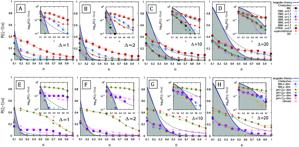
Figure 1: Variation of the estimates of $P\left((\xi-1)>\varepsilon\right)$ as function of the deviation $\varepsilon$. (A)-(D) show results for simulated processes with $M=100$ trajectories of $N=300$ points each, and for lag times $\Delta=1$, 2, 10, and 20, respectively. The insets show the results on semi-log scale. The statistical uncertainty is of the order of $0.01$. The parameters of the simulated stochastic processes are: $D=0.5$ for BM, $D_{H}=0.5$ for FBM, $D_{0}=0.5$ for SBM, $\tau_{0}=1$ for CTRW, $D_{0}=10$ for the superstatistical process, $\tau_{c}=10$ and $D_{\star}=0.2$ for DD. (E)-(H) show results for different experimental datasets for lag times $\Delta=1$, 2, 10, and 20, respectively. The insets again show the results on log-lin scale. The statistical uncertainty is of the order of $0.01$. For more details Appendix F.

For the special choices $\Delta=1$ and $\Delta=2$ the eigenvalues of $\Sigma(\Delta)$ can be calculated explicitly. This is relevant because for such low values of $\Delta$, the conclusions drawn from the TAMSD analysis of sufficiently long $T$ are statistically significant. For $\Delta=1$, the eigenvalues $\lambda_{j}(\Delta=1)=2D$ and therefore $\bar{\lambda}=4D$. Using this in (3) we get

$$P\left((\xi-1)>\varepsilon\right)\leq\exp\{-(N-1)\mathcal{H}(\varepsilon)/2\}.$$ (4)

For $\Delta=2$ the eigenvalues are given as (see Appendix C) $\lambda_{j}(\Delta=2)=D[4+4\cos(j\pi/[N-1])]$. This expression can then be used to obtain $\bar{\lambda}$ and thus $P\left((\xi-1)>\varepsilon\right)$ for $\Delta=2$. For other values of $\Delta$, the eigenvalues are obtained numerically eigen .

III Data sets for large-deviation analysis

We here describe the data used in our analysis below. These contain both BM and non-Brownian processes.

III.1 Simulated data

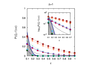
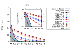
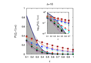
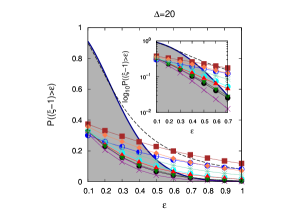
Figure 3: Variation of the estimates of $P\left((\xi-1)>\epsilon\right)$ with respect to $\epsilon$, for different simulated datasets with $N=300$, $M=10000$ and different values of $\Delta$.

Simulated data serve as benchmarks for the experimental data below. We simulate 100 trajectories each for different processes (Fig. 1 A-D). This number of trajectories is of the same order as in the experimental data sets. A larger set of 10,000 analyzed trajectories is presented in Fig. 3. In addition to BM, we simulate FBM, scaled Brownian motion (SBM), CTRW, superstatistical process, and diffusing-diffusivity (DD) process, see Appendix F for their exact definition. FBM mand68 is governed by the Langevin equation, driven by power-law correlated fractional Gaussian noise (FGN) $\eta_{\mathrm{H}}(t)$ with Hurst index $H$ ($0<H<1$), related to the anomalous diffusion exponent by $\alpha=2H$. SBM is characterized by the standard Langevin equation but with time-dependent diffusivity $D(t)\propto t^{\alpha-1}$ metz14 ; lim . CTRW is a renewal process with Gaussian jump lengths and long-tailed distribution $\psi(\tau)\simeq\tau^{(-1-\alpha)}$ ($0<\alpha<1$) of sojourn times between jumps scher75 ; montroll69 . For the simulated superstatistical process beck03 ; beck06 the diffusivity for each trajectory is drawn from a Rayleigh distribution. Finally, the DD process is governed by the Langevin equation with white Gaussian noise, but with a time-dependent, stochastic diffusivity, evolving as the square of an Ornstein-Uhlenbeck process with correlation time $\tau_{c}$ seno17 .

III.2 Beads tracked in aqueous solution

This data set (labeled "BM, x-dim" and "BM, y-dim" for the two directions) consists of 150 two-dimensional trajectories from single particle tracking of 1.2 $\mu$m-sized polystyrene beads in aqueous solution dieg18 . The time resolution of the data is 0.01 sec.

III.3 Beads tracked in mucin hydrogels

These data are from micron-sized tracer beads tracked in mucin hydrogels (MUC5AC with 1 wt% mucin) at pH=2 (labeled "pH=2, x-dim" and "pH=2, y-dim") and pH=7 (labeled "pH=7, x-dim" and "pH=7, y-dim") rubi17 . The imaging was performed at a rate of 30.3 frames per second. The pH=2 data set consists of 131 two-dimensional trajectories of 300 points each while the pH=7 data set consists of 50 trajectories of 300 points each.

III.4 Climate data

We also use daily temperature records over a 100 year period, after removing the annual cycle (these "anomalies" represent deviations from the corresponding mean daily temperature) mess16 . This data set consists of uninterrupted daily temperature recordings starting 1 January 1893 and are validated by the German Weather Service [Deutscher Wetterdienst (DWD), 2016]. The records were taken at the meteorological station at Potsdam Telegraphenberg (52.3813 latitude, 13.0622 longitude, 81 m above sea level).

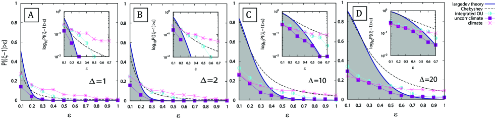
Figure 2: Variation of the estimates of $P\left((\xi-1)>\varepsilon\right)$ as function of $\varepsilon$ for the climate data, in comparison with the integrated OU process with correlation time of 5 steps. (A)-(D), respectively, show the results for $\Delta=1$, 2, 10, and 20. The insets show the results in semi-log scale. We observe that random shuffling of the temperature anomalies, before taking the cumulative sum to create the trajectories, removes the correlations in the data, and $P((\xi-1)>\varepsilon)$ behaves very similarly to BM ("uncorr climate").

IV Results

IV.1 Large deviations in simulated data sets

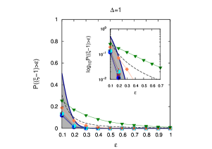
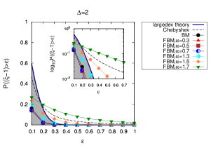
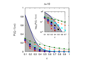
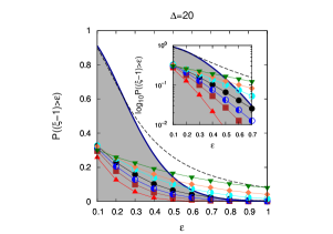
Figure 4: Variation of the estimates of $P\left((\xi-1)>\epsilon\right)$ with respect to $\epsilon$, for simulated FBM datasets of different anomalous diffusion exponent, with $N=300$, $M=10000$ and different values of $\Delta$. Superdiffusive FBM with large values of the anomalous diffusion exponent $\alpha$ fall out of the Brownian domain (gray-shaded region in the plot) for large values of the deviation parameter $\epsilon$.

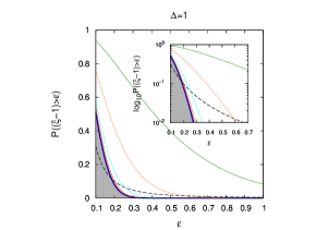
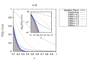
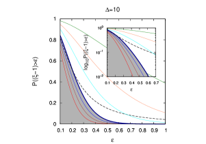
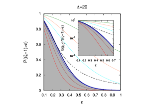
Figure 5: Comparison of the theoretical curves for the variation of $P\left((\xi-1)>\epsilon\right)$ with respect to $\epsilon$, for BM (labeled "largedev theory") and FBM with different anomalous diffusion exponent. The curve labeled "Chebyshev" is the theoretical curve of the Chebyshev inequality for BM. The different sub-figures are for $N=300$ and different values of the lag time, $\Delta$. Super-diffusive FBM with large values of the anomalous diffusion exponent $\alpha$ fall out of the Brownian domain (gray-shaded region in the plot), i.e. the theoretical bounds on the deviations of the normalized TAMSD for superdiffusive FBM are increasingly larger for larger values of $\alpha$. This supports the simulation results in Fig.4. No clear trend is observed for subdiffusive FBM at short lag times, although a trend similar to superdiffusive FBM appears at long lag times. This is, however, consistent with Fig. 4, where a clear trend for subdiffusive FBM is observed for the simulated datasets only at long lag times.

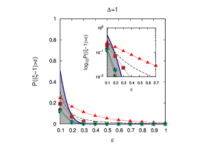
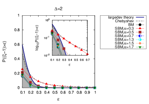
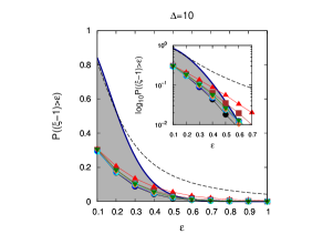
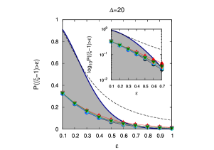
Figure 6: Variation of the estimates of $P\left((\xi-1)>\epsilon\right)$ with respect to $\epsilon$, for simulated SBM datasets of different anomalous diffusion exponent, with $N=300$, $M=10000$ and different values of $\Delta$. Subdiffusive SBM with small values of the anomalous diffusion exponent $\alpha$ fall out of the Brownian domain (gray-shaded region in the plot) for large values of the deviation parameter $\epsilon$, significantly at short lag times $\Delta$. This is in agreement with the behavior of the EB parameter reported for SBM in Ref. hadiseh , namely that for subdiffusive SBM the EB parameter (or equivalently the variance of the TAMSD) is larger for smaller values of the anomalous diffusion exponent. Moreover, for subdiffusive SBM, it was also reported in Ref. hadiseh that the EB parameter is larger for short lag times at fixed values of the anomalous diffusion exponent. This explains why subdiffusive SBM can be better distinguished from BM at small values of the lag time.

Fig. 1 A-D shows the comparison of the simulated data with the theoretical upper bounds (2) and (3) for BM, as function of the deviation $\varepsilon\in[0.1,1]$. Here each of the $M=100$ simulated trajectories was of length $N=300$. We see that, particularly at short $\Delta$, the theoretical bound (3) from large-deviation theory clearly distinguishes model classes and/or diffusive regimes. BM, subdiffusive FBM, and superdiffusive SBM clearly lie below the bound (3). In contrast, superdiffusive FBM with a large $H$ exponent, subdiffusive SBM with a small $\alpha$, CTRW, and random-diffusivity models (superstatistical and DD) clearly exceed the bound (3). Thus, non-Gaussianity (as realized for CTRW and the random-diffusivity processes) is not a unique criterion for the violation of the large-deviation bound. But according to these results the large-deviation method, for a given value of the scaling exponent $\alpha$, allows to distinguish FBM and SBM that both have a Gaussian PDF. At longer $\Delta$, in general, the theoretical bound (3) increases and thus $P\left((\xi-1)>\varepsilon\right)$ is below this bound for a larger range of $\varepsilon$. The large deviation method is surprisingly robust with respect to the number of analyzed trajectories, as can be seen from the marginal improvement of the results based on 10,000 trajectories in Fig. 3. Figs. 4 and 5 further analyze FBM and demonstrate the validity of the theoretical bound (14) derived for FBM. For further analysis of SBM see Fig. 6.

Chebyshev’s inequality (2) essentially provides the same bound as the one from large-deviation theory for short $\Delta$. However, at longer $\Delta$ it provides a much higher estimate than large-deviation theory, and it is unable to distinguish subdiffusive SBM with $\alpha=0.3$ from BM, as both lie below this bound. Moreover, for long $\Delta$ the probability $P\left((\xi-1)>\varepsilon\right)$ for all simulated processes lie either below or very close to the bound of Chebyshev’s inequality, rendering it ineffective in discerning different processes. Chebyshev’s inequality (2) lies above the large deviation bound (3), except for the cases $\Delta=1$ and 2 with small $\varepsilon$, when it is slightly below but still quite close to the bound set by (3).

IV.2 Large deviations in experimental data sets

IV.2.1 Beads tracked in aqueous solution

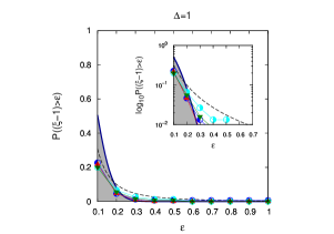
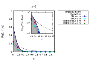
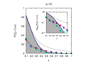
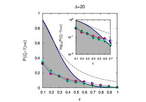
Figure 11: Variation of the estimates of $P\left((\xi-1)>\epsilon\right)$ with respect to $\epsilon$, for the datasets of polystyrene beads tracked in aqueous solution. The figure shows the results from the set of trajectories filtered using the JB test (labeled "BM,filtered,x-dim" and "BM,filtered,y-dim"), as compared to the full set of trajectories (labeled "BM,x-dim" and "BM,y-dim"). The parameters $N=300$ for all the datasets while $M=150$, $129$, and $125$ for the unfiltered sets, dataset labeled "BM,filtered,x-dim" and the dataset labeled "BM,filtered,y-dim" respectively.

Polysterene beads tracked in aqueous solution were analyzed in dieg18 using single-trajectory power spectral analysis, concluding that the data are consistent with BM. From Fig. 1 E-H it can be seen that the estimated probability $P\left((\xi-1)>\varepsilon\right)$ somewhat exceeds the theoretical bound (3) for BM. To understand this non-BM-like behavior shown in the large-deviation analysis we closely examined the motion of individual beads. Indeed, the displacement distributions of some beads showed non-Gaussian behavior, that we could attribute to bead-bead collisions as well as to imprecise localization of the bead center when the recorded tracks suffered from non-localized brightness. We removed the non-Gaussian trajectories using the JB test component-wise (see Appendix G). From the filtered data set ($M=129$ in $x$-direction and $M=125$ in $y$-direction) we see that the large-deviation analysis within the error bars is now consistent with BM (especially for $\Delta=1$, see Fig. 11). The large-deviation analysis is thus more sensitive to non-BM-like behavior than other methods dieg18 . We also note that the analysis based on Chebyshev’s inequality could not distinguish these features.

IV.2.2 Beads tracked in mucin hydrogels

The data sets ($M=131$ at pH=2 and $M=50$ at pH=7) consisting of beads tracked in mucin hydrogels show different trends of $P\left((\xi-1)>\varepsilon\right)$ depending on the pH values, as seen for $N=300$ in Fig. 1 E-H. Notably, for the beads tracked at pH=2 $P\left((\xi-1)>\varepsilon\right)$ remains significantly above the bound set by (3), particularly at short $\Delta$. This implies that the spread of the TAMSD is inconsistent with BM and hence the dynamics cannot be explained solely by BM. The data sets at pH=7 show significantly different behavior. We observe a clear distinction in the trend of $P\left((\xi-1)>\varepsilon\right)$ along the two directions of motion. Along the direction (labeled "x-dim") $P\left((\xi-1)>\varepsilon\right)$ remains slightly above the theoretical bound for BM from large-deviation theory for most of the range of $\varepsilon$ at $\Delta=1$ and $\Delta=2$, while it remains below the theoretical bound for the motion along the $y$-direction. As for the beads in aqueous solution, Chebyshev’s inequality provides a looser bound.

The mucin data sets were analyzed extensively in terms of Bayesian and other standard data analysis methods in mucin19 . The MSD and TAMSD exponents for the data at $\mathrm{pH}=2$ and 7 correspond to $\alpha=0.46$ and 0.36 and $\left<\beta\right>=1.09$ and 0.94, respectively. The angular bracket for $\beta$ denotes that these exponents were determined from the ensemble-averaged TAMSD. The discrepancy between the $\alpha$ and $\beta$ values suggest ergodicity breaking and hence a contribution from a model such as CTRW. For CTRW, the ensemble-averaged TAMSD scales with the total measurement time $T$ as a power-law metz14 . However, as shown in mucin19 , the ensemble-averaged TAMSD for the data sets at $pH=7$ showed no dependence on $T$, while the data sets at $pH=2$ showed a very weak dependence, ruling out CTRW as a model of diffusion. Moreover in the Bayesian analysis carried out in mucin19 BM, FBM and DD models were compared and relative probabilities were assigned to each of them, based on the likelihood for each trajectory to be consistent with a given process. It was observed that for both pH=2 and pH=7, and for most of the trajectories, both BM and FBM had high probabilities. On comparing the estimated Hurst index $H$ for the FBM, it was seen that for pH=7, $H\approx 0.5$ with a very small spread from trajectory to trajectory. In this sense, the pH=7 data seemed to be very close to BM. This was also confirmed independently by looking at $\beta$ extracted from the TAMSD. In contrast, the estimated $H$ for the pH=2 data showed a large spread in the range $0.3\leq H\leq 0.7$. These observations are now clearly supported by the results for $P\left((\xi-1)>\varepsilon\right)$, demonstrating that the data sets at $\mathrm{pH}=7$ are close to BM while the data sets at $\mathrm{pH}=2$ cannot be explained (solely) by BM. Thus, for this data set the large-deviation analysis again demonstrates its effectiveness in unveiling the physical origin of the stochastic time series.

IV.2.3 Climate data

The climate data were successfully modeled by an autoregressive fractionally integrated moving average model, more specifically, ARFIMA(1,d,0) with $d\approx 0.15$ mess16 ; kantz19 . ARFIMA(0,d,0) corresponds to FGN with $H=d+0.5$. It was found that the data, in addition to long-range correlations characteristic of FGN, exhibited short range correlations due to which ARFIMA(1,d,0) fitted the data better than ARFIMA(0, d,0). These short-range correlations could be explained by the average atmospheric circulation period of 4-5 days mess16 . For our tests of deviations of the TAMSD from the ensemble-averaged TAMSD, we construct FBM trajectories ($M=100$) of length $N=300$ by taking a cumulative sum of FGN. If the temperature anomalies could be described by ARFIMA(0,d,0), or, equivalently, by FGN, the cumulative sum would be FBM and hence should show a similar trend of $P\left((\xi-1)>\varepsilon\right)$, as seen for the simulated FBM processes in Fig. 1 A-D. That means that it remains below the theoretical upper bounds (2) and (3) for FBM, as long as the scaling exponent does not become too large. Alternatively, deviations of $P\left((\xi-1)>\varepsilon\right)$ from the trend exhibited by simulated FBM, particularly at $\alpha=1.3$ corresponding to $d=0.15$ reported in mess16 , would support the result in mess16 that ARFIMA(0,d,0) does not completely explain the data of surface temperature anomalies. This indeed turns out to be the case for $N=300$ in Fig. 1 E-H where we observe that $P\left((\xi-1)>\varepsilon\right)$ remains above the theoretical upper bound for BM from large-deviation theory, especially at short $\Delta$. Moreover, comparing with Fig. 1 A-D we clearly observe that $P\left((\xi-1)>\varepsilon\right)$ remains well above the theoretical upper bound (3) for BM for the climate data at sufficiently large values of $\varepsilon$, while it always remains below the bound for simulated FBM with $\alpha=1.3$ for all lag times. This corroborates the finding in mess16 that ARFIMA(0,d,0) (or equivalently FBM for the data constructed by taking the cumulative sum) cannot completely explain the climate data. In comparison, Chebyshev’s inequality (2) provides the same information for short lag times but fails to distinguish the climate data from corresponding simulated FBM for long $\Delta$, as this bound lies above the empirical probability $P\left((\xi-1)>\varepsilon\right)$ for both corresponding simulated FBM and climate data. In order to check whether the short-term correlations are indeed relevant, we create an artificially correlated process in the form of an integrated Ornstein-Uhlenbeck (OU) process, the results of which are shown in Fig. 2. With a correlation length of five steps the result of this OU process indeed leads to an $\varepsilon$ dependence of $P\left((\xi-1)>\varepsilon\right)$ that is very similar to the climate data’s. Conversely, as soon as we remove the correlations in the climate data by random reshuffling of the temperature anomalies, the large-deviation behavior becomes BM-like.

V Discussion and Conclusion

It is the purpose of time series analysis to detect the underlying physical process encoded in a measured trajectory, and thus to unveil the mechanisms governing the spreading of, e.g., viruses, vesicles, or signaling proteins in living cells or tissues. Recently considerable work has been directed to the characterization of stochastic trajectories using Bayesian analysis lomh18 ; lomh17 ; samu18 ; bayes ; bayes1 and machine learning gorka19 ; eich19 ; yael19 . Most of these methods are technically involved and expensive computationally. Moreover, the associated algorithms often heavily rely on data pre-processing gorka19 . To avoid overly expensive computations, it is highly advantageous to first go through a decision tree, to narrow down the possible families of physical stochastic mechanisms. For instance, one can eliminate ergodic versus non-ergodic or Gaussian versus non-Gaussian processes, etc. Here we analyze a new method based on large-deviation theory, concluding that it is a highly efficient and easy-to-use tool for such a characterization. We show how we can straightforwardly infer relevant information on the underlying physical process based on the theoretical bounds of the deviations of the TAMSD—routinely measured in single-particle-tracking experiments and supercomputing studies and easy to construct for any time-series such as daily temperature data—from the corresponding trajectory-average. Specifically, we demonstrate that this tool is able to detect the short-time correlations which effect non-FBM behavior in daily temperature anomalies, as well as the crossover from BM-like behavior at pH=7 to non-ergodic, non-BM-like at pH=2 for the mucin data, and the delicate sensitivity to non-Gaussian trajectories for beads in aqueous solution. We conclude from our analyses here that the large-deviation method would be an excellent basis for a first efficient screening of measured trajectories, before, if necessary, more refined methods are applied.

There are two seeming limitations to the large-deviation tool. First, it is easy to formulate this tool for one-dimensional trajectories, while the generalization to higher dimensions is not straightforward. However, as we demonstrated it can be used component-wise and, remarkably, can be used to probe the degree of isotropy of the data. In fact, from Fig. 1 E and F we concluded that the tracer bead motion in mucin at pH=7 was non-isotropic. In this sense, the one-dimensional definition of the large deviation tool is in fact an advantage. Second, it is not trivial to derive similar expressions as (3) for other stochastic processes. Here, numerical evaluations can be used instead. Moreover, in this case we can also use Chebyshev’s inequality, with the caveat that it works best at short lag times $\Delta$. Generally, the bound provided by the large-deviation theory is considerably more stringent than Chebyshev’s inequality, as demonstrated here.

We demonstrated that superdiffusive FBM with large $H$ values is outside the large-deviation bound. Superdiffusive FBM applied in mathematical finance are indeed in this range of $H$ values fin ; fin1 ; fin2 , and our large-deviation tool is therefore well suited for the analysis of such processes. We also showed that the large-deviation tool is able to uncover subtle correlations in the data, similarly to ARFIMA analyses applied mainly in mathematical finance and time series analysis. This similarity between the two methods strengthens the connections to physical models recently worked out between random coefficient autoregressive models and random-diffusivity models jakub .

The large-deviation test investigated here is a highly useful tool serving as an easy-to-implement and to-apply initial test in the decision tree for the classification of the physical mechanisms underlying measured time series from single particle trajectories.

Appendix A Description of the test algorithm

We take $M$ discretized trajectories of length $N$ of a given process (simulated or experimental). For the fixed time lag $\Delta$ we proceed as follows:

1. Calculate TAMSD for each trajectory according to the discrete equation, $\overline{\delta^{2}(\Delta)}=\sum_{j=1}^{N-\Delta}\left(X(j+\Delta)-X(j)\right)^{2}$.

2. Calculate the ensemble-averaged TAMSD $\left<\overline{\delta^{2}(\Delta)}\right>$.

3. For each trajectory calculate $\xi=\frac{\overline{\delta^{2}(\Delta)}}{\left<\overline{\delta^{2}(\Delta)}\right>}$.

4. Calculate the number of trajectories $M_{\epsilon}$ that satisfy the condition $\xi-1>\epsilon$ for a given $\epsilon$.

5. The empirical probability $P\left((\xi-1)>\epsilon\right)$ is calculated as $M_{\epsilon}/M$.

For a fixed value of $\epsilon$ and $\Delta$ we compare the empirical probability $P\left((\xi-1)>\epsilon\right)$ with the theoretical bounds given by the large-deviation theory and Chebyshev’s inequality. In our analysis we consider $\epsilon$ in the range $[0.1,1]$, and $\Delta\ll N$, namely $\Delta=1,2,10$ and $20$ points.

Appendix B Derivation of Chebyshev’s inequality for TAMSD of BM

Using the Markov Inequality, one can also show that for any random variable with mean $\mu$ and variance $\sigma^{2}$, and any positive number $k>0$, the following Chebyshev inequality (one-sided) holds savage

$$P\left(X-\mu\geq k\right)\leq\frac{\sigma^{2}}{\sigma^{2}+k^{2}}.$$ (5)

Here we derive Chebyshev’s inequality for the TAMSD statistic for BM. For the TAMSD it takes the following form

$$P\left((\xi-1)\geq k/\left<\overline{\delta^{2}(\Delta)}\right>\right)\leq\frac{\sigma^{2}}{\sigma^{2}+k^{2}},$$ (6)

where $\sigma^{2}=\mathrm{Var}\left(\overline{\delta^{2}(\Delta)}\right)=4\left<\overline{\delta^{2}(\Delta)}\right>^{2}\Delta/3N$, deng09 . Taking the notation $\varepsilon=k/\left<\overline{\delta^{2}(\Delta)}\right>$ one obtains the following

$$P\left((\xi-1)\geq\varepsilon\right) \leq \frac{4\left<\overline{\delta^{2}(\Delta)}\right>^{2}\Delta/3N}{4\left<\overline{\delta^{2}(\Delta)}\right>^{2}\Delta/3N+\epsilon^{2}\left<\overline{\delta^{2}(\Delta)}\right>^{2}}$$ (7)

$$= \frac{4\Delta}{4\Delta+3N\epsilon^{2}}.$$

Appendix C Eigenvalues of the covariance matrix of increments for BM

The $(N-\Delta)\times(N-\Delta)$ positive-definite covariance matrix ${\Sigma}(\Delta)$ for the vector of increments $\mathbb{Y}=(X(1+\Delta)-X(1),X(2+\Delta)-X(2),\ldots,X(N)-X(N-\Delta))$ takes the form

$$\Sigma(\Delta)=\begin{bmatrix}\sigma_{\Delta}(0)&\ \ \ \sigma_{\Delta}(1)\ \ \ &\ \ \ \sigma_{\Delta}(2)\ \ \ &\ \ \ldots\ \ &\ \ \ \ldots\ \ \ &\sigma_{\Delta}(N-\Delta-1)\\ \sigma_{\Delta}(1)&\sigma_{\Delta}(0)&\sigma_{\Delta}(1)&\ddots&&\vdots\\ \sigma_{\Delta}(2)&\sigma_{\Delta}(1)&\ddots&\ddots&\ddots&\vdots\\ \vdots&\ddots&\ddots&\ddots&\sigma_{\Delta}(1)&\sigma_{\Delta}(2)\\ \vdots&&\ddots&\sigma_{\Delta}(1)&\sigma_{\Delta}(0)&\sigma_{\Delta}(1)\\ \sigma_{\Delta}(N-\Delta-1)&\ldots&\ldots&\sigma_{\Delta}(2)&\sigma_{\Delta}(1)&\sigma_{\Delta}(0)\end{bmatrix},$$ (8)

with its elements given by

$$\sigma_{\Delta}(j)=\left\{\begin{array}[]{ll}2D(\Delta-j)&\textrm{$j\leq\Delta-1$}\\ 0&\textrm{$j>\Delta-1$}\\ \end{array}\right..$$ (11)

For the case of $\Delta=1$, the $(N-1)\times(N-1)$ covariance matrix ${\Sigma}(\Delta=1)$ has elements given by

$$\sigma_{\Delta=1}(j)=\left\{\begin{array}[]{ll}2D&\textrm{$j=0$}\\ 0&\textrm{$j>0$}\\ \end{array}\right..$$ (14)

Hence the matrix ${\Sigma}(\Delta=1)$ is a diagonal matrix with the constant main diagonal $2D$ and all zero entries outside the main diagonal. The characteristic polynomial of ${\Sigma}(\Delta=1)$ has the form

$$|{\Sigma}(\Delta=1)-\lambda I|=(\lambda-2D)^{N-1}$$

and roots $\lambda_{j}(\Delta=1)=2D,$ which are the eigenvalues of that matrix.

For the case $\Delta=2$ the $(N-2)\times(N-2)$ covariance matrix ${\Sigma}(\Delta=2)$ has elements given by

$$\sigma_{\Delta=2}(j)=\left\{\begin{array}[]{ll}2D(2-j)&\textrm{$j=0,1$}\\ 0&\textrm{$j>1$}\\ \end{array}\right..$$ (17)

Hence the matrix ${\Sigma}(\Delta=2)$ is a tridiagonal Toeplitz matrix. The formula forthe eigenvalues of such matrices is well known in the mathematical literature Bot05 ,

$$\lambda_{j}(\Delta=2)=D\left[4+4\cos\left(\frac{j\pi}{N-1}\right)\right].$$

Appendix D Large deviations of TAMSD for FBM

Taking Eq. (4.5) from gadj18 one can obtain the large deviation theory for FBM (see below for details of the stochastic process FBM). Namely, if we consider the vector of increments $\mathbb{Y}=(X(1+\Delta)-X(1),X(2+\Delta)-X(2),\ldots,X(N)-X(N-\Delta))$ of FBM with Hurst exponent $H$ and generalized diffusion coefficient $D_{H}$ then we have

$$P\left((\xi-1)>\epsilon\right)\leq\exp\left(-a\mathcal{H}\left(b\right)\right),$$ (18)

where $a=\frac{-2(N-\Delta)D_{H}^{2}S(\Delta,H,N)}{\overline{\lambda}(\Delta)^{2}}$ and $b=\frac{\overline{\lambda}(\Delta)\epsilon\Delta^{2H}}{D_{H}S(\Delta,H,N)}$. Here the function $\mathcal{H}(u)=1+u-\sqrt{1+2u}$ and $\bar{\lambda}(\Delta)=2\max\left\{\lambda_{j}(\Delta)\right\}$, where $\lambda_{j}(\Delta)$ ($j=1,2,...,N-\Delta$) are the eigenvalues of the $(N-\Delta)\times(N-\Delta)$ positive-definite covariance matrix ${\Sigma}(\Delta)$ for the vector of increments for FBM. Moreover the $S(\Delta,H,N)$ function is defined as

$$S(\Delta,H,N)=\sum_{i=0}^{N-\Delta-1}[(i+\Delta)^{2H}-2i^{2H}+|i-\Delta|^{2H}]^{2}.$$ (19)

It is worthwhile noting that for the FBM case the eigenvalues of the covariance matrix ${\Sigma}(\Delta)$ are not given in explicit form and need to be calculated numerically. Also note that Eq. (18) is independent of the generalized diffusion coefficient $D_{H}$ which gets canceled both in $a$ and $b$.

Appendix E Connection between Extreme value statistic and Large deviation theory

Consider $M$ discrete trajectories, $\{\{X_{1},X_{2},....,X_{N}\}_{1}$, $\{X_{1},X_{2},....,X_{N}\}_{2}$, $\ldots,,\{X_{1},X_{2},....,X_{N}\}_{M}\}$ of length $N$ of a given process. Let $Y_{j}$ be a statistic over each trajectory $j$, $j\in\{1,2,...,M\}$ (for instance, $Y$ could be the TAMSD). Large deviation theory deals with the probability that $P(Y>\epsilon)\leq\exp(-I)$, where $I$ is the rate function and $\epsilon$ is the deviation parameter. On the other hand, the extreme value statistic deals with the probability $P\left(\max\{Y_{1},Y_{2},..,Y_{M}\}>z\right)$. This probability can be written as

$$P\left(\max\{Y_{1},Y_{2},..,Y_{M}\}>z\right)$$

$$=1-P\left(\max\{Y_{1},Y_{2},..,Y_{M}\}\leq z\right)$$

$$=1-P(Y_{1}\leq z,Y_{2}\leq z,...,Y_{M}\leq z)$$

$$=1-\prod_{j=1}^{M}P(Y_{j}\leq z)$$

$$=1-P^{M}(Y_{1}\leq z)$$

$$=1-[1-P(Y_{1}>z)]^{M}.$$

The last three equalities come from the fact that the considered trajectories represent independent realizations of the same process.

Appendix F Simulated processes

For our analysis in the central Fig. 1 we simulate 100 trajectories each for different processes. The number of trajectories is of the same order as in the experimental datasets we analyze.

Brownian Motion (BM): Brownian motion is characterized by the Langevin equation in the overdamped limit as vankampen ; gardiner

$$\frac{dX(t)}{dt}=\sqrt{2D}\eta(t),$$ (20)

driven by the white Gaussian noise $\eta(t)$ with zero mean and autocorrelation function $\langle\eta(t_{1})\eta(t_{2})\rangle=\delta(t_{1}-t_{2})$. The parameter $D$ is the diffusion coefficient.

Fractional Brownian Motion (FBM): Fractional Brownian motion has been used to explain anomalous diffusion in a number of experiments hurs51 ; hurs65 ; weis09 ; wero09 ; klaf10 ; burn10 ; jeon11 ; weber10 , where the underlying process had long-range correlations. FBM mand82 ; mand68 is given by the Langevin equation

$$\frac{dX_{\mathrm{FBM}}(t)}{dt}=\eta_{\mathrm{H}}(t),$$ (21)

driven by the fractional Gaussian noise (fGn) $\eta_{\mathrm{H}}(t)$ with autocorrelation function

$$\langle\eta_{\mathrm{H}}(t_{1})\eta_{\mathrm{H}}(t_{2})\rangle=2H(2H-1)D_{H}\times|t_{1}-t_{2}|^{2(H-1)},$$ (22)

where $D_{H}$ is the generalized diffusion coefficient and $H$ is the Hurst index, which is related to the anomalous diffusion exponent $\alpha$ as $H=\alpha/2$.

Scaled Brownian Motion (SBM): Scaled Brownian motion has been used as a model of anomalous diffusion in numerous experiments weiss07 ; verk98 ; berl08 ; hoys06 ; dous92 ; boon13 , particularly those with fluorescence recovery after photobleaching saxt01 . SBM metz14 ; sbmralf is characterized by Eq. (20) but with a time-dependent diffusivity given by $D(t)=D_{0}t^{\alpha-1}$, with constant $D_{0}$ and the anomalous diffusion exponent $\alpha$. The parameter $0<\alpha<1$ leads to a subdiffusive MSD while $1<\alpha<2$ leads to a superdiffusive MSD.

Continuous Time Random Walk (CTRW): The subdiffusive CTRW has been used to describe a number of experiments scher75 ; weitz04 ; chaikin11 ; krapf11 ; swinney93 exhibiting anomalous diffusion. It is a renewal process with Gaussian jumps with an asymptotic power-law distributed waiting time between successive jumps scher75 ; montroll69 ; metz14 . The asymptotic probability density function (PDF) of the waiting time $\tau$ is given by $\psi(\tau)\approx\tau_{0}^{\alpha}\tau^{(-1-\alpha)}$, where $0<\alpha<1$ is the anomalous diffusion exponent of the MSD. We refer to hans07 for details of the simulation.

Superstatistical process: By a superstatistical process beck03 ; beck06 we mean a process which is defined by Eq. (20) where the diffusion coefficient is a random variable, that is, there exists a distribution of diffusivities over the tracers in a single particle tracking experiment. The convolution of such distributions of diffusivities with a Gaussian distribution can give rise to non-Gaussian displacement distributions routinely observed in many experiments hapc09 ; gran12 ; gran14 ; schw15d ; rubi17 ; cher19 ; gupt18 ; tong16 ; java16 . As in many of these experiments, the diffusivity has a Rayleigh-like distribution, for our simulated superstatistical process we applied the Rayleigh distribution for the diffusivity,

$$p(D)=\frac{D}{D_{0}^{2}}\exp{\left(-\frac{D^{2}}{2D_{0}^{2}}\right)},$$ (23)

where $D_{0}$ is the scale parameter of the Rayleigh distribution and is related to the mean $\langle D\rangle=D_{0}\sqrt{(\pi/2)}$.

Diffusing Diffusivity (DD): The minimal DD model can be expressed as the set of stochastic differential equations seno17

$$\dfrac{dX_{DD}(t)}{dt}=\sqrt{2D(t)}\eta_{1}(t),$$ (24a)

$$D(t)=Y^{2}(t),$$ (24b)

$$\dfrac{dY(t)}{dt}=-\dfrac{Y(t)}{\tau_{c}}+\sigma\eta_{2}(t),$$ (24c)

where the time dependent diffusion coefficient is defined as the square of the Ornstein-Uhlenbeck process $Y(t)$ and $\tau_{c}$ is the relaxation time to the stationary limit uhle30 . $\eta_{1}(t)$ and $\eta_{2}(t)$ are independent white Gaussian noise with zero mean and unit variance. In the long time, stationary limit the diffusion coefficients are distributed roughly exponentially seno17 ,

$$p(D)=(\pi DD_{\star})^{-1/2}\exp[-D/D_{\star}],$$ (25)

where $D_{\star}=\sigma^{2}\tau_{c}$. The TAMSD for this DD model grows linearly with lag time but the PDF of the process is non-Gaussian (Laplacian) for times less than the relaxation time $\tau_{c}$, and it crosses over to a Gaussian PDF for $t\gg\tau_{c}$. This behavior was seen in a number of experiments gran12 ; gran14 .

Appendix G The Jarque-Bera test for Gaussianity

In statistics, the Jarque-Bera (JB) test is a goodness-of-fit test used to recognize if the sample data have the skewness and kurtosis matching the Gaussian distribution. The test statistic is always nonnegative. If it is far from zero, then we can suspect, the data are not from the Gaussian distribution. The JB statistic for a random sample $x_{1},x_{2},...,x_{n}$ is defined as follows jb ,

$$JB=\frac{n}{6}\left(S^{2}+\frac{1}{4}(K-3)^{2}\right),$$ (26)

where $S$ and $K$ are the empirical skewness and kurtosis, respectively.

In the literature, the JB test based on the JB statistic is considered as one of the most effective tests for Gaussianity. It is especially useful in the problem of recognition between heavy- and light-tailed (Gaussian) distributions of the data.

Appendix H Supplementary figures

We here present additional figures that we refer to in the main text.

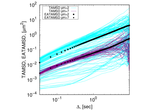
Figure 7: TAMSD (and its ensemble average EATAMSD) plot considering 2-dimensional motion of beads tracked in Mucin hydrogel at $pH=2$ and $pH=7$. There are $50$ trajectories at $pH=7$ and $131$ trajectories at $pH=2$. Each trajectory consists of $N=300$. The estimated $\left<\beta\right>=\{1.09,0.94\}$ for $pH=\{2,7\}$ respectively mucin19 .

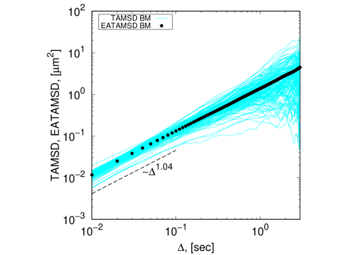
Figure 8: TAMSD (and its ensemble average EATAMSD) plot considering 2-dimensional motion of beads tracked in aqueous solution. There are $150$ trajectories with $N=300$.

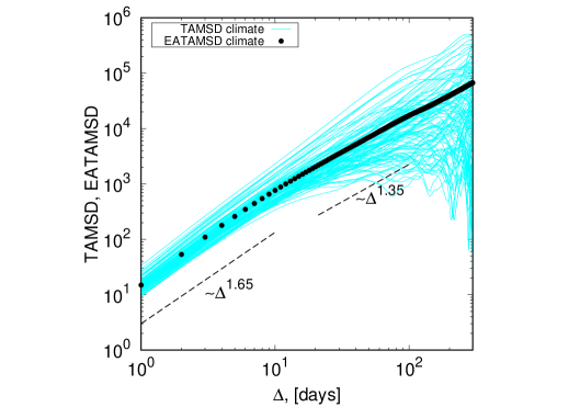
Figure 9: TAMSD (and its ensemble average EATAMSD) plot of climate data after taking cumulative sum of the temperature anomalies. There are $100$ trajectories with $N=300$.

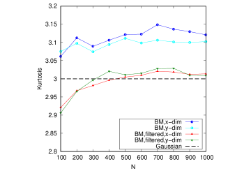
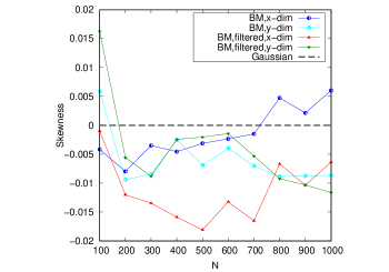
Figure 10: Average (over the trajectories) kurtosis (left) and average skewness (right) as function of $N$ for trajectories of polystyrene beads tracked in aqueous solution. This plot shows how the set of trajectories filtered using the JB test (labeled "BM,filtered,x-dim" and "BM,filtered,y-dim") shows Gaussian behavior (particularly with respect to the kurtosis), as compared to the full set of trajectories (labeled "BM,x-dim" and "BM,y-dim").

References

- (1) F. Höfling, and T. Franosch, Anomalous transport in the crowded world of biological cells, Rep. Prog. Phys. 76, 046602 (2013).
- (2) K. Nørregaard, R. Metzler, C. Ritter, K. Berg-Sørensen, and L. Oddershede, Manipulation and motion of organelles and single molecules in living cells, Chem. Rev. 117, 4342 (2017).
- (3) A. V. Weigel, B. Simon, M. M. Tamkun, and D. Krapf, Ergodic and Nonergodic Processes Coexist in the Plasma Membrane as Observed by Single-Molecule Tracking, Proc. Natl. Acad. Sci. U.S.A. 108, 6438 (2011).
- (4) S. M. A. Tabei, S. Burov, H. Y. Kim, A. Kuznetsov, T. Huynh, J. Jureller, L. H. Philipson, A. R. Dinner, and N. F. Scherer, Intracellular transport of insulin granules is a subordinated random walk, Proc. Natl. Acad. Sci. USA 110, 4911 (2013).
- (5) E. Barkai, Y. Garini, and R. Metzler, Strange Kinetics of Single Molecules in Living Cells, Phys. Today 65(8), 29 (2012).
- (6) I. M. Sokolov, Models of anomalous diffusion in crowded environments, Soft Matter 8, 9043 (2012).
- (7) R. Metzler, J.-H. Jeon, A. G. Cherstvy, and E. Barkai, Anomalous diffusion models and their properties: non-stationarity, non-ergodicity, and ageing at the centenary of single particle tracking, Phys. Chem. Chem. Phys. 16, 24128 (2014).
- (8) G. Seisenberger, M. U. Ried, T. Endreß, H. Büning, M. Hallek, and C. Bräuchle, Real-Time Single-Molecule Imaging of the Infection Pathway of an Adeno-Associated Virus, Science 294, 1929 (2001).
- (9) J. F. Reverey, J.-H. Jeon, H. Bao, M. Leippe, R. Metzler, and C. Selhuber-Unkel, Superdiffusion dominates intracellular particle motion in the supercrowded space of pathogenic Acanthamoeba castellanii, Sci. Rep. 5, 11690 (2015).
- (10) C. Di Rienzo, V. Piazza, E. Gratton, F. Beltram and F. Cardarelli, Probing short-range protein Brownian motion in the cytoplasm of living cells, Nat. Commun. 5, 5891 (2014).
- (11) S. Burov, R. Metzler, and E. Barkai, Aging and non-ergodicity beyond the Khinchin theorem, Proc. Natl. Acad. Sci. USA 107, 13228 (2010).
- (12) D. Krapf, E. Marinari, R. Metzler, G. Oshanin, X. Xu and A. Squarci Power spectral density of a single Brownian trajectory: what one can and cannot learn from it, New J. Phys. 20, 023029 (2018).
- (13) D. Krapf, N. Lukat, E. Marinari, R. Metzler, G. Oshanin, C. Selhuber-Unkel, A. Squarcini, L. Stadler, M. Weiss, and X. Xu, Spectral Content of a Single Non-Brownian Trajectory, Phys. Rev. X 9, 011019 (2019).
- (14) Y. Meroz and I. M. Sokolov, A toolbox for determining subdiffusive mechanisms, Phys. Rep. 573, 1 (2015).
- (15) S. Thapa, M. A, Lomholt, J. Krog, A. G. Cherstvy and R. Metzler Bayesian analysis of single-particle tracking data using the nested-sampling algorithm: maximum-likelihood model selection applied to stochastic-diffusivity data, Phys. Chem. Chem. Phys. 20, 29018 (2018).
- (16) C. Mark, C. Metzner, L. Lautscham, P. L. Strissel, R. Strick, and Ben Fabry, Bayesian model selection for complex dynamic systems, Nat. Comms. 9, 1803 (2018).
- (17) F. Persson, M. Lindén, C. Unoson, and J. Elf, Extracting intracellular diffusive states and transition rates from single-molecule tracking data, Nat. Meth. 10, 265 (2013).
- (18) G. Muñoz-Gil, M. A. Garcia-March, C. Manzo, J. D. Martín-Guerrero, and M. Lewenstein, Single trajectory characterization via machine learning, New J. Phys. 22, 013010 (2020).
- (19) B. V. Gnedenko, The theory of probability (American Mathematical Society, Providence RI, 2005).
- (20) R. Savage, Probability, Inequalities of the Tchebycheff Type, J. Res. Natl. Bur. Stand. - B. Math. Math. Phys. 65B, 211 (1961).
- (21) L. Fang, K. Ma, R. Li, Z. Wang, and H. Shi, A Statistical Approach to Estimate Imbalance-Induced Energy Losses for Data-Scarce Low Voltage Networks, IEEE Trans. Power Syst. 34, 2825 (2019).
- (22) X. Xue, C. Li, S. Cao, J. Sun, and L. Liu, Fault Diagnosis of Rolling Element Bearings with a Two-Step Scheme Based on Permutation Entropy and Random Forests, Entropy 21, 96 (2019).
- (23) G. V. G. Baranoski, J. G. Rokne, and G. Xu, Applying the exponential Chebyshev inequality to the nondeterministic computation of form factors, J. Quant. Spectrosc. Radiat. Transf. 69, 447 (2001).
- (24) H. Cramér, Sur un nouveau théorème limite dans la théorie des probabilités, in: Colloque consacré à la théorie des probabilités, vol. 3 (Hermann, Paris, 1938).
- (25) M. D. Donsker, S. R. S. Varadhan, Asymptotic evaluation of certain Markov process expectations for large time I, Comm. Pure Appl. Math. 28, 1 (1975).
- (26) M. D. Donsker, S. R. S. Varadhan, Asymptotic evaluation of certain Markov process expectations for large time IV, Comm. Pure Appl. Math. 36, 183 (1983).
- (27) J. Feng and T. G. Kurtz, Large deviations for stochastic processes, Mathematical Surveys and Monographs (American Mathematical Society, Providence RI, 2006).
- (28) A. Dembo and O. Zeitouni, Large deviations techniques and applications, Vol. 38 (Springer, Berlin, 2009).
- (29) S. Y. Novak, Extreme value methods with applications to finance (Chapman Hall/CRC Press, New York, 2011).
- (30) F. R. Ragone, J. Wouters and F. Bouchet, Computation of extreme heat waves in climate models using a large deviation algorithm, Proc. Natl. Acad. Sci. U. S. A. 115, 24 (2018).
- (31) H. Touchette, The large deviation approach to statistical mechanics, Phys. Rep. 478, 1 (2009).
- (32) H. Djellout, A. Guillin, and Y. Samoura, Estimation of the realized (co-)volatility vector: Large deviations approach, Stoch. Proc. Applic. 127, 2926 (2017).
- (33) B. Bercu and A. Richou, Large deviations for the Ornstein-Uhlenbeck process without tears, Statist. Probab. Lett. 123, 45 (2017).
- (34) V. Fasen and P. Roy, Stable random fields, point processes and large deviations, Stochast. Proc. Applic. 126, 832 (2016).
- (35) R. Kumar and L. Popovic, Large deviations for multi-scale jump-diffusion processes, Stochast. Proc. Applic. 127, 1297 (2017).
- (36) J. Gajda and M. Magdziarz, Large deviations for subordinated Brownian motion and applications, Stochast. Proc. Applic. 88, 149 (2014).
- (37) E. Barkai and S. Burov, Packets of diffusing particles exhibit universal exponential tails, Phys. Rev. Lett. 124, 060603 (2020).
- (38) D. Qi and A. J. Majda, Using machine learning to predict extreme events in complex systems, Proc. Natl. Acad. Sci. U.S.A. 117, 52 (2019).
- (39) M. K. Tippett, C. Lepore and J. E. Cohen, More tornadoes in the most extreme U.S. tornado outbreaks, Science, 354, 1419 (2016).
- (40) S. Ornes,How does climate change influence extreme weather? Impact attribution research seeks answers, Proc. Natl. Acad. Sci. U.S.A. 115, 8232 (2018).
- (41) J. Gajda, A. Wyłomańska, H. Kantz, A. V. Chechkin, and G. Sikora, Large deviations of time-averaged statistics for Gaussian processes, Statist. Probab. Lett. 143, 47 (2018).
- (42) C. B. Moler and C. W. Stewart, An algorithm for generalized matrix eigenvalue problems, SIAM J. Numer. Anal. 10, 241 (1973).
- (43) B. B. Mandelbrot and W. J. van Ness, Fractional Brownian motions, fractional noises and applications, SIAM Rev. 10, 422 (1968).
- (44) S. C. Lim and S. V. Muniandy, Self-similar Gaussian processes for modeling anomalous diffusion, Phys. Rev. E 66, 021114 (2002).
- (45) E. W. Montroll and G. H. Weiss, Random Walks on Lattices. III. Calculation of First-Passage Times with Application to Exciton Trapping on Photosynthetic Units, J. Math. Phys. 10, 753 (1969).
- (46) H. Scher and E. W. Montroll, Anomalous transit-time dispersion in amorphous solids, Phys. Rev. B 12, 2455 (1975).
- (47) C. Beck and E. G. D. Cohen, Superstatistics, Physica A 322, 267 (2003).
- (48) C. Beck, Superstatistical Brownian motion, Prog. Theor. Phys. Suppl. 162, 29 (2006).
- (49) A. V. Chechkin, F. Seno, R. Metzler, and I. M. Sokolov, Brownian yet non-Gaussian diffusion: from superstatistics to subordination of diffusing diffusivities, Phys. Rev. X 7, 021002 (2017).
- (50) C. E. Wagner, B. S. Turner, M. Rubinstein, G. H. McKinley, and K. Ribbeck, A rheological study of the association and dynamics of MUC5AC gels, Biomacromolecules 18, 3654 (2017).
- (51) M. Massah, and H. Kantz, Confidence intervals for time averages in the presence of long-range correlations, a case study on Earth surface temperature anomalies, Geophys. Res. Lett. 43, 9243 (2016).
- (52) A. G. Cherstvy, S. Thapa, C.E. Wagner, and R. Metzler, Non-Gaussian, non-ergodic and non-Fickian diffusion of tracers in mucin hydrogels, Soft Matter 15, 2526 (2019).
- (53) P. G. Meyer and H. Kantz, Inferring characteristic timescales from the effect of autoregressive dynamics on detrended fluctuation analysis , New J. Phys. 21, 033022 (2019).
- (54) J. Krog, L. H. Jacobsen, F. W. Lund, D. Wüstner, and M. A. Lomholt, Bayesian model selection with fractional Brownian motion, J. Stat. Mech. 2018, 093501 (2018).
- (55) J. Krog and M. A. Lomholt, Bayesian inference with information content model check for Langevin equations, Phys. Rev. E. 96, 062106 (2017).
- (56) S. Bo, F. Schmidt, R. Eichhorn, and G. Volpe, Measurement of Anomalous Diffusion Using Recurrent Neural Networks, Phys. Rev. E. 100, 010102 (2019).
- (57) N. Granik, E. Nehme, L. E. Weiss, M. Levin, M. Chein, E. Perlson, Y. Roichman, and Yoav Shechtman, Single particle diffusion characterization by deep learning, Biophys. J. 117, 185 (2019).
- (58) G. Rodríguez, Modeling Latin-American stock and Forex markets volatility: Empirical application of a model with random level shifts and genuine long memory, North Amer. J. Econ. Fin. 42, 393 (2017).
- (59) J. Proelss, D. Schweizer, and V. Seiler, The economic importance of rare earth elements volatility forecasts, Int. Rev. Fin. Anal., in press; DOI:10.1016/j.irfa.2019.01.010.
- (60) F. N. Zargar and D. Kumar, Long range dependence in the Bitcoin market: A study based on high-frequency data, Physica A 515, 625 (2019).
- (61) J. Ślȩzak, K. Burnecki, and R. Metzler, Random coefficient autoregressive processes describe Brownian yet non-Gaussian diffusion in heterogeneous systems, New J. Phys. 21, 073056 (2019)
- (62) W. Feller, An introduction to probability theory and its applications, Vol. 2 (Wiley, New York, 1966).
- (63) W. Deng and E. Barkai, Ergodic properties of fractional Brownian-Langevin motion, Phys. Rev. E. 79, 011112 (2009).
- (64) C. M. Jarque and A. K. Bera, A test for normality of observations and regression residuals, Internat. Statist. Rev. 55, 163 (1987).
- (65) A. Böttcher and S. M. Grudsky, Spectral Properties of Banded Toeplitz Matrices, (SIAM, Philadelphia 2005).
- (66) N. G. van Kampen, Stochastic processes in physics and chemistry (North Holland, Amsterdam, 1989).
- (67) W. T. Coffey and Y. P. Kalmykov, The Langevin equation (World Scientific, Singapore, 2012).
- (68) H. E. Hurst, Long-term storage capacity of reservoirs, Trans. Am. Soc. Civ. Eng. 116, 770 (1951).
- (69) H. W. Hurst, R. O. Black, and Y. M. Simaika , Long Term Storage: An Experimental Study, (Constable, London, UK 1965).
- (70) J. Szymanski and M. Weiss, Elucidating the origin of anomalous diffusion in crowded fluids, Phys. Rev. Lett. 103, 038102 (2009).
- (71) M. Magdziarz, A. Weron, K. Burnecki, and J. Klafter, Fractional Brownian motion versus the continuous-time random walk: A simple test for subdiffusive dynamics, Phys. Rev. Lett. 103, 180602 (2009).
- (72) M. Magdziarz and J. Klafter, Detecting origins of subdiffusion: p-variation test for confined systems, Phys. Rev. E. 82, 011129 (2010).
- (73) K. Burnecki and J. Klafter, Fractional Lévy stable motion can model subdiffusive dynamics, Phys. Rev. E. 82, 021130 (2010).
- (74) J. -H. Jeon, V. Tejedor, S. Burov, E. Barkai, C. Selhuber-Unkel, K. Berg-Sørensen, L. Oddershede, and R. Metzler, In Vivo Anomalous Diffusion and Weak Ergodicity Breaking of Lipid Granules, Phys. Rev. Lett. 106 048103, (2011).
- (75) S. C. Weber, A. J. Spakowitz, and J. A. Theriot, Bacterial chromosomal loci move subdiffusively through a viscoelastic cytoplasm, Phys. Rev. Lett. 104, 238102 (2010).
- (76) B. B. Mandelbrot, The fractal geometry of nature, (W. H. Freeman, New York, 1982).
- (77) G. Guigas, C. Kalla, and M. Weiss, The degree of macromolecular crowding in the cytoplasm and nucleoplasm of mammalian cells is conserved, FEBS Lett. 581, 5094 (2007).
- (78) N. Periasmy and A. S. Verkman, Analysis of fluorophore diffusion by continuous distributions of diffusion coefficients: Application to photobleaching measurements of multicomponent and anomalous diffusion, Biophys. J. 75, 557 (1998).
- (79) J. Wu and M. Berland, Propagators and time-dependent diffusion coefficients for anomalous diffusion, Biophys. J. 95, 2049 (2008).
- (80) J. Szymaski, A. Patkowski, J. Gapiski, A. Wilk, and R. Hoyst, Movement of proteins in an environment crowded by surfactant micelles: anomalous versus normal diffusion, J. Phys. Chem. B. 110, 7367 (2006).
- (81) P. P. Mitra, P. N. Sen, L. M. Schwartz, and P. Le Doussal, Diffusion propagator as a probe of the structure of porous media, Phys. Rev. Lett. 68, 3555 (1992).
- (82) J. F. Lutsko and J. P. Boon, Microscopic theory of anomalous diffusion based on particle interactions, Phys. Rev. E. 88, 022108 (2013).
- (83) M. J. Saxton, Anomalous subdiffusion in fluorescence photobleaching recovery: a Monte Carlo study, Biophys. J. 81, 2226 (2001).
- (84) J.-H. Jeon, A. V. Chechkin, and R. Metzler, Scaled Brownian motion: a paradoxical process with a time dependent diffusivity for the description of anomalous diffusion, Phys. Chem. Chem. Phys. 16, 15811 (2014).
- (85) I. Y. Wong, M. L. Gardel, D. R. Reichman, E. R. Weeks, M. T. Valentine, A. R. Bausch, and D. A. Weitz, Anomalous diffusion probes microstructure dynamics of entangled F-actin networks, Phys. Rev. Lett. 92, 178101 (2004).
- (86) Q. Xu, L. Feng, R. Sha, N. C. Seeman, and P. M. Chaikin, Subdiffusion of a sticky particle on a surface, Phys. Rev. Lett. 106, 228102 (2011).
- (87) T. H. Solomon, E. R. Weeks, and H. L. Swinney, Observation of anomalous diffusion and Lévy flights in a two-dimensional rotating flow, Phys. Rev. Lett. 71, 3975 (1993).
- (88) H. C. Fogedby, Langevin equations for continuous time Lévy flights, Phys. Rev. E. 50, 1657 (1994).
- (89) D. Kleinhans and R. Friedrich, Continuous-time random walks: Simulation of continuous trajectories, Phys. Rev. E. 76, 061102 (2007).
- (90) B. Wang, S. M. Anthony, S. C. Bae, and S. Granick, Anomalous yet Brownian, Proc. Natl. Acad. Sci. U. S. A. 106, 15160 (2009).
- (91) B. Wang, J. Kuo, S. C. Bae, and S. Granick, When Brownian diffusion is not Gaussian, Nat. Mater. 11, 481 (2012).
- (92) S. Hapca, J. W. Crawford, and I. M. Young, Anomalous diffusion of heterogeneous populations characterized by normal diffusion at the individual level, J. Roy. Soc. Interface 6, 111 (2009).
- (93) J. Guan, B. Wang, and S. Granick, Even hard-sphere colloidal suspensions display Fickian yet non-Gaussian diffusion, ACS Nano 8, 3331 (2014).
- (94) D. Wang, C. He, M. P. Stoykovich, and D. K. Schwartz, Nanoscale topography influences polymer surface diffusion, ACS Nano 9, 1656 (2015).
- (95) W. He, H. Song, Y. Su, L. Geng, B. J. Ackerson, H. B. Peng, and P. Tong, Dynamic heterogeneity and non-Gaussian statistics for acetylcholine receptors on live cell membrane, Nat. Comm. 7, 11701 (2016).
- (96) J.-H. Jeon, M. Javanainen, H. Martinez-Seara, R. Metzler, and I. Vattulainen, Protein crowding in lipid bilayers gives rise to non-Gaussian anomalous lateral diffusion of phospholipids and proteins, Phys. Rev. X. 6, 021006 (2016).
- (97) S. Gupta, J. U. De Mel, R. M. Perera, P. Zolnierczuk, M. Bleuel, A. Faraone, and G. J. Schneider, Dynamics of phospholipid membranes beyond thermal undulations, J. Phys. Chem. Lett. 9, 2956 (2018).
- (98) A. G. Cherstvy, O. Nagel, C. Beta, and R. Metzler, Non-Gaussianity, population heterogeneity, and transient superdiffusion in the spreading dynamics of amoeboid cells, Phys. Chem. Chem. Phys. 20, 23034 (2018).
- (99) G. E. Uhlenbeck and L. S. Ornstein, On the theory of the Brownian motion, Phys. Rev. 36, 823 (1930).
- (100) H. Safdari, A. G. Cherstvy, A. V. Chechkin, F. Thiel, I. M. Sokolov, and R. Metzler, Quantifying the non-ergodicity of scaled Brownian motion, J. Phys. A: Math. Theor. 48, 375002 (2015).