First passage time moments of asymmetric Lévy flights

Abstract

We investigate the first-passage dynamics of symmetric and asymmetric Lévy flights in a semi-infinite and bounded intervals. By solving the space-fractional diffusion equation, we analyse the fractional-order moments of the first-passage time probability density function for different values of the index of stability and the skewness parameter. A comparison with results using the Langevin approach to Lévy flights is presented. For the semi-infinite domain, in certain special cases analytic results are derived explicitly, and in bounded intervals a general analytical expression for the mean first-passage time of Lévy flights with arbitrary skewness is presented. These results are complemented with extensive numerical analyses.

1 Introduction

Lévy flights (LFs) correspond to a class of Markovian random walk processes that are characterised by an asymptotic power-law form for the distribution of jump lengths with a diverging variance [1, 2, 3, 4, 5]. The name "Lévy flight" was coined by Benoît Mandelbrot, in honour of his formative teacher, French mathematician Paul Pierre Lévy [1, 6]. The trajectories of LFs are statistical fractals [1], characterised by local clusters interspersed with occasional long jumps. Due to their self-similar character, LFs display "clusters within clusters" on all scales. This emerging fractality [1, 2, 3, 7] makes LFs efficient search processes as they sample space more efficiently than normal Brownian motion: in one and two dimensions Brownian motion is recurrent and therefore oversamples the search space. LFs, in contrast, reduce oversampling due to the occurrence of long jumps [8, 9, 10, 11, 12, 13, 14, 15, 16, 17, 18]. As search strategies LFs were argued to be additionally advantageous as, due to their intrinsic lack of length scale they are less sensitive to time-changing environments [15]. Concurrently in an external bias LFs may lose their lead over Brownian search processes [19, 20]. LFs were shown to underlie human movement behaviour and thus lead to more efficient spreading of diseases as compared to diffusive, Brownian spreading [21, 22, 23]. LFs appear as traces of light beams in disordered media [24], and in optical lattices the divergence of the kinetic energy of single ions under gradient cooling are related to Lévy-type fluctuations [25]. Finally, we mention that Lévy statistics were originally identified in stock market price fluctuations by Mandelbrot and Fama [26, 27], see also [28].

Mathematically, LFs are based on $\alpha$-stable distributions (or Lévy distributions) [29, 30] which emerge as limiting distributions of sums of independent, identically distributed (i.i.d.) random variables according to the generalised central limit theorem—that is, they have their own, well-defined domains of attraction [2, 3, 29, 30]. The characteristic function of an $\alpha$-stable process, which is a continuous-time counterpart of an LF, is given as [31, 32]

$$\hat{\ell}_{\alpha,\beta}(k,t)=\int\limits_{-\infty}^{\infty}\ell_{\alpha,\beta}(x,t)\rme^{ikx}\mathrm{d}x=\exp\Big{(}-tK_{\alpha}|k|^{\alpha}[1-i\beta\mathrm{sign}(k)\omega(k,\alpha)]+i\mu kt\Big{)},$$ (1)

with the stability index (Lévy index) $\alpha$ that is allowed to vary in the interval $0<\alpha\leq 2$. Moreover, equation (1) includes the skewness parameter $\beta$ with $-1\leq\beta\leq 1$, and $K_{\alpha}>0$ is a scale parameter. The shift parameter $\mu$ can be any real number, and the phase factor $\omega$ is defined as

$$\omega(k,\alpha)=\left\{\begin{array}[]{ll}\tan(\frac{\pi\alpha}{2}),&\alpha\neq 1\\ -\frac{2}{\pi}\ln|k|,&\alpha=1\end{array}\right..$$ (2)

Physically, the parameter $\mu$ accounts for the constant drift in the system. In this paper, we consider the first-passage time moments in the absence of a drift, $\mu=0$. The stable index $\alpha$ is responsible for the slow decay of the far asymptotics of the $\alpha$-stable probability density function (PDF). Indeed, symmetric $\alpha$-stable distributions in absence of a drift ($\beta=\mu=0$) have the characteristic function $\exp(-K_{\alpha}|k|^{\alpha}t)$, whose asymptote in real space has the power-law form $\simeq K_{\alpha}t|x|^{-1-\alpha}$ ("heavy tail" or "long tail"), and thus absolute moments $\langle|x|^{\delta}\rangle$ of order $\delta<\alpha$ exist [2, 3, 31, 33]. The scale parameter $K_{\alpha}$ (along with the stable index $\alpha$) physically sets the size of the LF-jumps. The skewness $\beta$ may be related to an effective drift or counter-gradient effects [34, 35]. LFs have been applied to explain diverse complex dynamic processes, where scale-invariant phenomena take place or can be suspected [1, 29]. According to the generalised central limit theorem, each $\alpha$-stable distribution with fixed $\alpha<2$ attracts distributions with infinite variance which decay with the same law as the attracting stable distribution. A particular case of a stable density is the Gaussian for $\alpha=2$, for which moments of all orders exist. We note that the Gaussian law not only attracts distributions with finite variance but also distributions decaying as $\simeq|x|^{-3}$; that is, distributions, whose variance is marginally infinite [36, 30]. To fit real data, in particular, in finance, which feature heavy-tailed distributions on intermediate scales, however, with finite variance, the concept of the truncated LFs has been introduced according to which the truncation of the heavy tail at larger scales is achieved either by an abrupt cutoff [37], an exponential cutoff [38], or by a steeper power-law decay [39, 40, 41].

The efficiency of the spatial exploration and search properties of a stochastic process is quantified by the statistics of the "first-hitting" or the "first-passage" times [42, 43, 44, 45]. For instance, the first-passage of a stock price crossing a given threshold level serves as a trigger to sell the stock. The event of first-hitting would correspond to the event when exactly a given stock price is reached. Of course, when stock prices change continuously (as is the case for a continuous Brownian motion) both first-passage and first-hitting are equivalent [44]. In contrast, for an LF with the propensity of long, non-local jumps the two definitions lead to different results. In general, the first-passage will be realised earlier: it is more likely that an LF jumps across a point in space [46] effecting so-called "leapovers" [47, 48]. For a foraging albatross, for instance, the first-hitting would correspond to the moment when it locates a single, almost point-like, forage fish. The first-passage would correspond to the event when the albatross crosses the circumference of a large fish shoal. We here focus on the first-passage time statistic of LFs, and our main objective is the study of the moments of the first-passage time for asymmetric LFs in semi-infinite and bounded domains. Such moments can be conveniently used to quantify search processes. The most commonly used moment is the mean first-passage time (MFPT) $\langle\tau\rangle=\int_{0}^{\infty}\wp(\tau)\tau\mathrm{d}\tau$ in terms of the first-passage time density $\wp(\tau)$ (see below), when it exists. However, other definitions such as the mean of the inverse first-passage time, $\langle 1/\tau\rangle$ have also been studied [19, 20]. More generally, the spectrum of fractional order first-passage time moments $\langle\tau^{q}\rangle$ is important to characterise the underlying stochastic process from measurements. The characteristic times $\langle\tau\rangle$ and $\langle 1/\tau\rangle$ thus correspond to $q=1$ and $q=-1$, respectively. In what follows we study the behaviour of the spectrum of $\langle\tau^{q}\rangle$ as function of the LF parameters.

A set of classical results exists for the first-passage time properties of LFs in a semi-infinite domain. In particular, [49, 50] used limit theorems of i.i.d. random variables to obtain the asymptotic behaviour of the first-passage time distribution. Based on a continuous-time storage model the first-passage time of a general class of Lévy processes was studied in [51]. By applying the laws of ladder processes the asymptotic of the first-passage time distribution of Lévy stable processes was investigated in [52]. After becoming clear that LFs have essential applications in different fields of science, several remarkable results were established. Thus, in [53] it was reported that one-dimensional symmetric random walks with independent increments in half-space have universal property. Also [54] showed that the survival probability of symmetric LFs in a one-dimensional half-space with an absorbing boundary at the origin is independent of the stability index $\alpha$ and thus displays universal behaviour. It is by now well-known that the mentioned results are a consequence of the celebrated Sparre Andersen theorem [55, 56]. Accordingly, the PDF of the first-passage times of any symmetric and Markovian jump process originally released at a fixed point $x_{0}$ from an absorbing boundary in semi-infinite space has the universal asymptotic scaling $\wp(\tau)\simeq\tau^{-3/2}$ [43, 46, 47, 48]. This law has been confirmed by extensive numerical simulations of the first-passage time PDF [47] and the associated survival probability [57] of symmetric LFs within a Langevin dynamic approach (see below). Furthermore, the asymptotic of the survival probability of symmetric, discrete-time LFs was studied in [58, 59], and based on the space-fractional diffusion equation the first-passage time PDF and the survival probability was investigated in [60]. Starting from the Skorokhod theorem, the Sparre Andersen theorem could be successfully reproduced analytically [48, 60]. Other analytical and numerical results that concern the first-passage properties of asymmetric LFs in a semi-infinite domain are the following. For one-sided $\alpha$-stable process ($0<\alpha<1$ with $\beta=1$) the first-passage time PDF and the MFPT was studied in [48]. In [47] the authors used Langevin dynamic simulations to study the asymptotic behaviour of the first-passage time PDF of extremal two-sided ($1<\alpha<2$ with $\beta=-1$) $\alpha$-stable laws. Moreover, by employing the space-fractional diffusion equation the first-passage time PDF and the survival probability of extremal two-sided $\alpha$-stable laws ($1<\alpha<2$ with $\beta=1$) and the asymptotic of the first-passage PDF of general, asymmetric LFs was investigated in [60].

With respect to the first-passage from a finite interval a number of classical results for symmetric $\alpha$-stable process were reported in a series of papers in the 1950s and 1960s. To name a few, the MFPT of one-dimensional symmetric ($\beta=0$) Cauchy ($\alpha=1$) processes [61], the MFPT of two-dimensional Brownian motion [62], and the MFPT of one-dimensional symmetric $\alpha$-stable process with stability index $0<\alpha<1$ were studied [63]. Moreover, for the case $0<\alpha\leq 2$ and $\beta=0$ the results of the first-passage probability in one dimension [64], the MFPT as well as the second moment of the first-passage time PDF in $N$ dimensions were reported [65]. One-sided $\alpha$-stable processes with $0<\alpha<1$ and $\beta=1$ in a finite interval were studied with the help of arc-sine laws of renewal theory in [66] and by using the harmonic measure of a Markov process in [67]. A closed form for the MFPT by potential theory method was obtained in [68]. For completely asymmetric LFs the first-passage time of the two-sided exit problem was addressed in [68, 69, 70, 71, 72, 73]. The residual MFPT of LFs in a one-dimensional domain was investigated in [74]. We also mention that necessary and sufficient conditions for the finiteness of the moments of the first-passage time PDF of a general class of Lévy processes in terms of the characteristics of the random process $X(t)$ were shown by [75]. Additionally, harmonic functions in a Markovian setting were defined by the mean value property concerning the distribution of the process being stopped at the first exit time of a domain [76]. Finally, the authors in [77], by using the Green’s function of a Lévy stable process [78], obtained the non-negative harmonic functions for the stable process killed outside a finite interval, allowing the computation of the MFPT.

We also mention that various problems of the first-passage for symmetric and asymmetric $\alpha$-stable processes, as well as for two- and three-dimensional motions, were considered by different approaches. These include Monte-Carlo simulations and the Fredholm integral equation [79, 80], Langevin dynamics simulations [81, 82], fractional Laplacian operators [83, 84], eigenvalues of the fractional Laplacian [85], and the backward fractional Fokker-Plank equation [86]. Moreover, noteworthy are simulations of radial LFs in two dimensions [7], the effect of Lévy noise on a gene transcriptional regulatory system [87], the study of the mean exit time and the escape probability of one- and two-dimensional stochastic dynamical systems with non-Gaussian noises [88, 89, 90]. The tail distribution of the first-exit time of LFs from a closed $N$-ball of radius $R$ in a recursive manner was constructed in [91]. Very recently, extensive simulations of the space-fractional diffusion equation and the Langevin equation were used to investigate the first-passage properties of asymmetric LFs in a semi-infinite domain in [60]. In the same work application of the Skorokhod theorem allowed to derive a closed form for the first-passage time PDF of extremal two-sided $\alpha$-stable laws with stability index $1<\alpha<2$ and skewness $\beta=\pm 1$, as well as the first-passage time PDF asymptotic for asymmetric Lévy stable laws with arbitrary skewness parameter $\beta$.

The first part of this paper, based on our previous results in [60], is devoted to the study of fractional order moments of the first-passage time PDF of LFs in a semi-infinite domain for symmetric ($0<\alpha<2$ with $\beta=0$), one-sided ($0<\alpha<1$ with $\beta=1$), extremal two-sided ($1<\alpha<2$ with $\beta=\pm 1$), and a general form ($\alpha\in(0,2]$ with $\beta\in[-1,1]$, excluding $\alpha=1$ with $\beta\neq 0$) $\alpha$-stable laws. Specifically we obtain a closed-form solution for the fractional moments of the first-passage time PDF for one-sided and extremal two-sided $\alpha$-stable processes, and we report the conditions for the finiteness of the fractional moments of the first-passage time PDF for the full class of $\alpha$-stable processes. We also present comparisons with numerical solutions of the space-fractional diffusion equation. In the second part we derive a closed form of the MFPT of asymmetric LFs in a finite interval by solving the fractional differential equation for the moments of the first-passage time PDF. In particular cases we present a comparison between our analytical results with the numerical solution of the space-fractional diffusion equation as well as simulations of the Langevin equation. Moreover, we show that the MFPT of LFs in a finite interval is representative for the first-passage time PDF by analysing the associated coefficient of variation.

The structure of the paper is as follows. In section 2 we introduce the space-fractional diffusion equation in a finite interval. In section 3, the numerical schemes for the space-fractional diffusion equation and the Langevin equation are presented. We set up the corresponding formalism to study the moments of the first-passage time PDF in section 4. Section 5 then presents the analytic and numerical results of the fractional moments of the first-passage time PDF for symmetric, one-sided, and extremal two-sided stable distributions in semi-infinite domains. We derived a closed-form solution of the MFPT for asymmetric LFs in a finite interval in section 6 and compare with the numerical solution of the space-fractional diffusion equation and the Langevin dynamics simulations. We draw our conclusions in section 7, and details of the mathematical derivations are presented in the appendices.

2 Space-fractional diffusion equation in a finite domain

Fractional derivatives have been shown to be convenient when formulating the generalised continuum diffusion equations for continuous time random walk processes with asymptotic power-law asymptotes for both the distributions of sojourn times and jump lengths [4, 5, 92, 93, 94]. We here use the space-fractional diffusion equation for infinite domains and its extension to semi-infinite and finite domains to describe the dynamics of LFs. From a probabilistic point of view, the basic Caputo and Riemann-Liouville derivatives of order $\alpha\in(0,2)$ can be viewed as generators of LFs interrupted on crossing a boundary [46, 48, 95]. The corresponding equation to describe LFs has the following expression for the PDF $P_{\alpha,\beta}(x,t|x_{0})$

$$\frac{\partial P_{\alpha,\beta}(x,t|x_{0})}{\partial t}=K_{\alpha}\,D^{\alpha}_{x}P_{\alpha,\beta}(x,t|x_{0})$$ (3)

with initial condition $P_{\alpha,\beta}(x,0|x_{0})=\delta(x-x_{0})$, where $D_{x}^{\alpha}$ is the space-fractional operator for motion confined to the interval $[-L,L]$,

$$D^{\alpha}_{x}f(x)=L_{\alpha,\beta}\,\,{}_{-L}D_{x}^{\alpha}f(x)+R_{\alpha,\beta}\,\,{}_{x}D_{L}^{\alpha}f(x).$$ (4)

Here ${}_{-L}D_{x}^{\alpha}$ and ${}_{x}D_{L}^{\alpha}$ are left and right space-fractional derivatives, respectively. Let us first consider the case $\alpha\neq 1$ and $-1\leq\beta\leq 1$. We use the Caputo form of the fractional operators defined by $(n-1<\alpha<n)$ as [96]

$$_{-L}D_{x}^{\alpha}f(x)=\frac{1}{\Gamma(n-\alpha)}\int\limits_{-L}^{x}\frac{f^{(n)}(\zeta)}{(x-\zeta)^{\alpha-n+1}}\,\mathrm{d}\zeta,$$ (5)

and

$$_{x}D_{L}^{\alpha}f(x)=\frac{(-1)^{n}}{\Gamma(n-\alpha)}\int\limits_{x}^{L}\frac{f^{(n)}(\zeta)}{(\zeta-x)^{\alpha-n+1}}\,\mathrm{d}\zeta.$$ (6)

$L_{\alpha,\beta}$ and $R_{\alpha,\beta}$ are the left and right weight coefficients, defined as [97, 98]

$$L_{\alpha,\beta}=-\frac{1+\beta}{2\cos(\frac{\alpha\pi}{2})},\quad R_{\alpha,\beta}=-\frac{1-\beta}{2\cos(\frac{\alpha\pi}{2})}.$$ (7)

For the case $\alpha=1$ and $\beta=0$ we have $L_{1,0}=R_{1,0}=1/\pi$, and the left and right space-fractional operators respectively read [99]

$${}_{-L}D_{x}^{1}f(x)=-\int\limits_{-L}^{x}\frac{f^{(1)}(\zeta)}{x-\zeta}\mathrm{d}\zeta,$$ (8)

$${}_{x}D_{L}^{1}f(x)=\int\limits_{x}^{L}\frac{f^{(1)}(\zeta)}{\zeta-x}\mathrm{d}\zeta.$$ (9)

In the present paper, we do not consider the particular case $\alpha=1$, $\beta\neq 0$ since it cannot be described in terms of a space-fractional operator.

We end this section by adding a remark concerning our choice of the Caputo form of the fractional derivatives (5) and (6): it is known that there are different equivalent definitions of the fractional Laplacian operator in unbounded domains [100], which in general case loose their equivalence in bounded domains, see, e.g., [101, 102, 103]. Such ambiguity, however, does not hold in case of the first passage problem when absorbing boundary conditions are applied. In this case it is easy to verify that the Riemann-Liouville derivatives are equivalent to the Caputo derivatives [99, 96]. However, in the general case for bounded domains the use of the Caputo derivative is preferrable in applied problems for the following reason: the Riemann-Liouville approach leads to boundary conditions, which do not have known direct physical interpretation [96], and thus the left and right Riemann-Liouville derivatives might be singular at the lower and upper boundaries, respectively, as discussed in [97] in detail—a problem circumvented by defining the fractional derivative in the Caputo sense.

3 Numerical schemes

Apart from analytical approaches to be specified below, to determine the moments of the first-passage time PDF of $\alpha$-stable processes we will employ two numerical schemes based on the space-fractional diffusion equation and the Langevin equation for LFs. We here detail their specific implementation.

3.1 Diffusion description

Numerical methods to solve space-fractional diffusion equations are relatively sparse, and the majority of the publications are based on the finite-difference scheme [104, 105] and finite-element methods [106, 107, 108] as well as the spectral approach [109, 110]. In this paper, we use the finite-difference scheme to solve the space-fractional diffusion equation introduced in the preceding section. Here we only outline the essence of the method and refer to [60] for further details. The computationally most straightforward method arises from the forward-difference scheme in time on the left hand side of equation (3),

$$\frac{\partial}{\partial t}f(x_{i},t_{j})=\frac{f^{j+1}_{i}-f^{j}_{i}}{\Delta t}+\mathcal{O}(\Delta t),$$ (10)

where $f^{j}_{i}=f(x_{i},t_{j})$, $x_{i}=(i-I/2)\Delta x$, and $t_{j}=j\Delta t$, where $\Delta x$ and $\Delta t$ are step sizes in position and time, respectively. The $i$ and $j$ are non-negative integers, $i=0,1,2,\ldots,I$, and $\Delta x=2L/I$. Similarly, $j=0,1,2,\ldots,J-1$, $t_{0}=0$, $t_{J}=t$, and $\Delta t=t/J$. Absorbing boundary conditions for the determination of the first-passage events imply $f_{0}^{j}=f_{I}^{j}=0$ for all $j$. The integrals on the right hand side of equation (3) are discretised as follows. For $0<\alpha<1$,

$$\int\limits_{-L}^{x_{i}}\frac{f^{(1)}(\zeta,t_{j})}{(x_{i}-\zeta)^{\alpha}}\mathrm{d}\zeta=\displaystyle\sum_{k=1}^{i}\frac{f^{j}_{k}-f^{j}_{k-1}}{\Delta x}\int\limits_{x_{k-1}}^{x_{k}}\frac{1}{(x_{i}-\zeta)^{\alpha}}\mathrm{d}\zeta+\mathcal{O}(\Delta x^{2-\alpha})$$ (11)

for the left derivative, and

$$\int\limits_{x_{i}}^{L}\frac{f^{(1)}(\zeta,t_{j})}{(\zeta-x_{i})^{\alpha}}\mathrm{d}\zeta=\displaystyle\sum_{k=i}^{I-1}\frac{f^{j}_{k+1}-f^{j}_{k}}{\Delta x}\int\limits_{x_{k}}^{x_{k+1}}\frac{1}{(\zeta-x_{i})^{\alpha}}\mathrm{d}\zeta+\mathcal{O}(\Delta x^{2-\alpha})$$ (12)

for the right derivative. This scheme is called L1 scheme and is an efficient way to approximate the Caputo derivative of order $0<\alpha<1$ [111, 112, 113] with error estimate $\mathcal{O}(\Delta x^{2-\alpha})$. For the case $1<\alpha<2$ the suitable method to discretise the Caputo derivative is the L2 scheme [111, 113, 114], namely,

$$\int\limits_{-L}^{x_{i}}\frac{f^{(2)}(\zeta,t_{j})}{(x_{i}-\zeta)^{\alpha-1}}\mathrm{d}\zeta=\displaystyle\sum_{k=1}^{i}\frac{f^{j}_{k+1}-2f^{j}_{k}+f^{j}_{k-1}}{(\Delta x)^{2}}\int\limits_{x_{k-1}}^{x_{k}}\frac{1}{(x_{i}-\zeta)^{\alpha-1}}\mathrm{d}\zeta+\mathcal{O}(\Delta x)$$ (13)

for the left derivative, and

$$\int\limits_{x_{i}}^{L}\frac{f^{(2)}(\zeta,t_{j})}{(\zeta-x_{i})^{\alpha-1}}\mathrm{d}\zeta=\displaystyle\sum_{k=i}^{I-1}\frac{f^{j}_{k+1}-2f^{j}_{k}+f^{j}_{k-1}}{(\Delta x)^{2}}\int\limits_{x_{k}}^{x_{k+1}}\frac{1}{(\zeta-x_{i})^{\alpha-1}}\mathrm{d}\zeta+\mathcal{O}(\Delta x)$$ (14)

for the right derivative. We note that the truncation error of the L2 scheme is $\mathcal{O}(\Delta x)$ [114, 115]. For the special case $\alpha=1$ and $\beta=0$ we approximate the derivative in space with the backward difference scheme

$$\int\limits_{-L}^{x_{i}}\frac{f^{(1)}(\zeta,t_{j})}{x_{i}-\zeta}\mathrm{d}\zeta=\displaystyle\sum_{k=1}^{i}\frac{f^{j}_{k}-f^{j}_{k-1}}{\Delta x}\frac{2}{2(i-k)+1}+\mathcal{O}(\Delta x^{2})$$ (15)

for the left derivative, and with a forward difference scheme

$$\int\limits_{x_{i}}^{L}\frac{f^{(1)}(\zeta,t_{j})}{\zeta-x_{i}}\mathrm{d}\zeta=\displaystyle\sum_{k=i}^{I-1}\frac{f^{j}_{k}-f^{j}_{k+1}}{\Delta x}\frac{2}{2(k-i)+1}+\mathcal{O}(\Delta x^{2})$$ (16)

for the right derivative. We note that here the truncation error is the order $\mathcal{O}(\Delta x^{2})$. By substitution of equations (10) to (16) into (3) we obtain

$$\mathbf{A}f^{j+1}=\mathbf{B}f^{j},$$ (17)

where the coefficients $\mathbf{A}$ and $\mathbf{B}$ have matrix form of dimension $(I+1)\times(I+1)$ and $j=0,1,2,\ldots,J-1$. In the numerical scheme for the setup used in our numerical simulations (see section 4 and figure 1 below) the initial condition $f(x,0)=\delta(x-x_{0})$ at $x_{0}=L-d$ is approximated as

$$f(x_{i},0)=\left\{\begin{array}[]{ll}(\Delta x)^{-1},&i=(2L-d)/\Delta x\\ 0,&\mbox{otherwise}\end{array}\right..$$ (18)

In the next step, the time evolution of the PDF is obtained by applying the absorbing boundary conditions $f_{0}^{j}=f_{I}^{j}=0$ for all $j$.

3.2 Langevin dynamics

The fractional diffusion equation (3) can be related to the LF Langevin equation [57, 116, 117]

$$\frac{\mathrm{d}}{\mathrm{d}t}x(t)=K_{\alpha}^{1/\alpha}\zeta(t),$$ (19)

where $\zeta(t)$ is Lévy noise characterised by the same $\alpha$ and $\beta$ parameters as the space-fractional operator (3) and with unit scale parameter. The Langevin equation (19) provides a microscopic (trajectory-wise) representation of the space-fractional diffusion equation (3). Therefore, from an ensemble of trajectories generated from equation (19), it is possible to estimate the time-dependent PDF whose evolution is described by equation (3). In numerical simulations, LFs can be described by the discretised form of Langevin equation

$$x(t+\Delta t)=x(t)+K_{\alpha}^{1/\alpha}(\Delta t)^{1/\alpha}\zeta_{t},$$ (20)

where $\zeta_{t}$ stands for the sequence of i.i.d. $\alpha$-stable random variables with unit scale parameter [31, 118] and identical index of stability $\alpha$ and skewness $\beta$ as in equation (19). Relation (20) is exactly the Euler-Maruyama approximation [119, 120, 121] to a general $\alpha$-stable Lévy process.

From the trajectories $x(t)$, see equations (19) and (20), it is also possible to estimate the first-passage time $\tau$ as

$$\tau=\min\{t:|x(t)|\geqslant L\}.$$ (21)

From the ensemble of first-passage times, it is then possible to obtain the survival probability $S(t)$, which is the complementary cumulative density of first-passage times. More precisely, the initial condition is $S(0)=1$, and at every recorded first-passage event at time $\tau_{i}$, $S(t)$ is decreased by the amount $1/N$ where $N$ is the overall number of recorded first-passage events.

4 First passage time properties of $\alpha$-stable processes

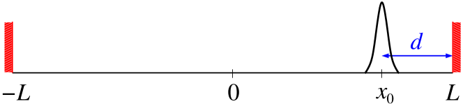
Figure 1: Schematic of our setup. In the interval of length $2L$ the initial condition is given by a $\delta$-distribution located at $x_{0}$, which is chosen the distance $d$ away from the right boundary. At both interval boundaries we implement absorbing boundary conditions, that is, when the particle hits the boundaries or attempts to move beyond them, it is absorbed.

For an $\alpha$-stable random process, the survival probability and the first-passage time are observable statistical quantities characterising the stochastic motion in bounded domains with absorbing boundary conditions. In the following, we investigate the properties of the first-passage time moments in a semi-infinite and finite interval for symmetric and asymmetric $\alpha$-stable laws underlying the space-fractional diffusion equation. In addition a comparison with the Langevin approach and with analytical expressions for the MFPT of LFs in a finite interval is presented. To this end, we use the setup shown in figure 1, in which the absorbing boundaries are located at $-L$ and $L$, and the centre point of the initial $\delta$-distribution is located the distance $d$ away from the right boundary.

The survival probability that up until time $t$ a random walker remains "alive" within the interval $[-L,L]$ is defined as [43, 45]

$$S(t|x_{0})=\int\limits_{-L}^{L}P_{\alpha,\beta}(x,t|x_{0})\mathrm{d}x,$$ (22)

Recall that $P_{\alpha,\beta}(x,t|x_{0})$ is the PDF of an LF confined to the interval $[-L,L]$ which starts at $x_{0}$. The associated first-passage time PDF reads

$$\wp(t|x_{0})=-\frac{\mathrm{d}S(t|x_{0})}{\mathrm{d}t}.$$ (23)

The first-passage time PDF satisfies in particular the normalisation

$$\int\limits_{0}^{\infty}\wp(t|x_{0})\,\mathrm{d}t=1,$$ (24)

and the positive integer moments of this random variable are defined as

$$\langle\tau^{m}\rangle(x_{0})=\int\limits_{0}^{\infty}t^{m}\wp(t|x_{0})\mathrm{d}t=\int\limits_{0}^{\infty}mt^{m-1}S(t|x_{0})\mathrm{d}t,\,\,\,\,m=1,2,\dots.$$ (25)

Employing the Laplace transform,

$$f(t)\div\mathscr{L}\{f(t);s\}=\int\limits_{0}^{\infty}\rme^{-st}f(t)\mathrm{d}t,$$ (26)

we obtain

$$\langle\tau^{m}\rangle(x_{0})=(-1)^{m}\frac{\partial^{m}}{\partial s^{m}}\Big{[}\wp(s|x_{0})\Big{]}\Big{|}_{s=0}.$$ (27)

Conversely, following the procedure suggested in [83], by substitution of equation (22) into equation (25) we get

$$\langle\tau^{m}\rangle(x_{0})=\int\limits_{0}^{\infty}mt^{m-1}\int\limits_{-L}^{L}P_{\alpha,\beta}(x,t|x_{0})\mathrm{d}x\mathrm{d}t.$$ (28)

Applying the backward space-fractional Kolmogorov operator $D^{\alpha}_{x_{0}}$ in a finite domain (see details in A),

$$D^{\alpha}_{x_{0}}f(x_{0})=R_{\alpha,\beta}\,{}_{-L}D_{x_{0}}^{\alpha}f(x_{0})+L_{\alpha,\beta}\,{}_{x_{0}}D_{L}^{\alpha}f(x_{0}),$$ (29)

to both sides of equation (28),

$$D^{\alpha}_{x_{0}}\langle\tau^{m}\rangle(x_{0})=\int\limits_{0}^{\infty}mt^{m-1}\int\limits_{-L}^{L}D^{\alpha}_{x_{0}}P_{\alpha,\beta}(x,t|x_{0})\mathrm{d}x\mathrm{d}t,$$ (30)

and using the corresponding backward Kolmogorov equation

$$\frac{\partial P_{\alpha,\beta}(x,t|x_{0})}{\partial t}=K_{\alpha}\,D^{\alpha}_{x_{0}}P_{\alpha,\beta}(x,t|x_{0}),$$ (31)

we get

$$D^{\alpha}_{x_{0}}\langle\tau^{m}\rangle(x_{0})=\frac{m}{K_{\alpha}}\int\limits_{0}^{\infty}t^{m-1}\frac{\partial}{\partial t}\int\limits_{-L}^{L}P_{\alpha,\beta}(x,t|x_{0})\mathrm{d}x\mathrm{d}t.$$ (32)

In the limit $m=1$,

$$D^{\alpha}_{x_{0}}\langle\tau\rangle(x_{0})=\frac{1}{K_{\alpha}}\left(\int\limits_{-L}^{L}P_{\alpha,\beta}(x,\infty|x_{0})\mathrm{d}x-\int\limits_{-L}^{L}P_{\alpha,\beta}(x,0|x_{0})\mathrm{d}x\right).$$ (33)

Then, by including the initial condition of the density function $P_{\alpha,\beta}(x,0|x_{0})=\delta(x-x_{0})$, where $x_{0}\in[-L,L]$, we get the functional relation

$$D^{\alpha}_{x_{0}}\langle\tau\rangle(x_{0})=-\frac{1}{K_{\alpha}}$$ (34)

for the MFPT. This result is similar to equation (41) in [83], except that instead of a symmetric Riesz-Feller operator we here employ a more general form of the fractional derivative operator $D_{x_{0}}^{\alpha}$ which is called backward space-fractional Kolmogorov operator in a finite domain. We note that in comparison with the forward space-fractional derivative defined by equation (4) in equation (29) the left and right weight coefficients are exchanged.

For the case $m=2$, we have

$$D^{\alpha}_{x_{0}}\langle\tau^{2}\rangle(x_{0})=\frac{2}{K_{\alpha}}\int\limits_{0}^{\infty}t\frac{\partial}{\partial t}\int\limits_{-L}^{L}P_{\alpha,\beta}(x,t|x_{0})\mathrm{d}x\mathrm{d}t.$$ (35)

Changing the order of integration,

$$D^{\alpha}_{x_{0}}\langle\tau^{2}\rangle(x_{0})=\frac{2}{K_{\alpha}}\int\limits_{-L}^{L}\int\limits_{0}^{\infty}t\frac{\partial}{\partial t}P_{\alpha,\beta}(x,t|x_{0})\mathrm{d}t\mathrm{d}x,$$ (36)

integrating by parts in the inner integral,

$$D^{\alpha}_{x_{0}}\langle\tau^{2}\rangle(x_{0})=-\frac{2}{K_{\alpha}}\int\limits_{-L}^{L}\int\limits_{0}^{\infty}P_{\alpha,\beta}(x,t|x_{0})\mathrm{d}t\mathrm{d}x,$$ (37)

and, once again, changing the order of integration, we find

$$D^{\alpha}_{x_{0}}\langle\tau^{2}\rangle(x_{0})=-\frac{2}{K_{\alpha}}\int\limits_{0}^{\infty}\int\limits_{-L}^{L}P_{\alpha,\beta}(x,t|x_{0})\mathrm{d}x\mathrm{d}t.$$ (38)

Calling on equation (28) with $m=1$, we obtain the functional relation

$$D^{\alpha}_{x_{0}}\langle\tau^{2}\rangle(x_{0})=-\frac{2}{K_{\alpha}}\langle\tau\rangle(x_{0})$$ (39)

for the second moment of the first-passage time PDF.

More generally, by using this recursion relation one can write

$$D^{\alpha}_{x_{0}}\langle\tau^{m}\rangle(x_{0})=-\frac{m}{K_{\alpha}}\langle\tau^{m-1}\rangle(x_{0}),\,\,\,m=1,2,\ldots.$$ (40)

By applying $D^{\alpha}_{x_{0}}$ on both sides,

$$(D^{\alpha}_{x_{0}})^{2}\langle\tau^{m}\rangle(x_{0})=-\frac{m}{K_{\alpha}}D^{\alpha}_{x_{0}}\langle\tau^{m-1}\rangle(x_{0}),$$ (41)

and with equation (40) we have

$$(D^{\alpha}_{x_{0}})^{2}\langle\tau^{m}\rangle(x_{0})=\frac{m(m-1)}{{K_{\alpha}}^{2}}\langle\tau^{m-2}\rangle(x_{0}).$$ (42)

By repeating this procedure, we derive

$$(D^{\alpha}_{x_{0}})^{m}\langle\tau^{m}\rangle(x_{0})=\frac{(-1)^{m}\Gamma(1+m)}{{K_{\alpha}}^{m}}.$$ (43)

This equation is the generalisation of the result obtained in [83] for symmetric LFs (see equation (44) there).

5 First passage time properties of LFs in a semi-infinite domain

In this section, we investigate the first-passage time properties of LFs in a semi-infinite domain. The motion starts at $x_{0}$, and the boundary is located at $x=L$, in such a way that in our setup $L-x_{0}=d$. In order to reproduce numerically the results for semi-infinite domain with the scenario shown in figure 1, we employ $L$ as well as $x_{0}$, as large as possible in order to allow a constant $d$ ($L=10^{12}$ in our simulations).

5.1 Symmetric LFs in a semi-infinite domain

For a semi-infinite domain with an absorbing boundary condition, as said above it is well known that the first-passage time density for any symmetric jump length distribution in a Markovian setting has the universal Sparre Andersen scaling $\wp(t)\simeq t^{-3/2}$ [43, 55, 56]. In the theory of a general class of Lévy processes, that is, homogeneous random processes with independent increments, there exists a theorem, that provides an analytical expression for the PDF of first-passage times in a semi-infinite interval, often referred to as the Skorokhod theorem [32, 122]. Based on this theorem the asymptotic expression for the first-passage time PDF of symmetric $\alpha$-stable laws is [48]

$$\wp(t)\sim\frac{d^{\alpha/2}}{\alpha\sqrt{\pi K_{\alpha}}\Gamma{(\alpha/2)}}t^{-3/2},$$ (44)

which specifies an exact expression for the prefactor in the Sparre Andersen scaling law. The existence of this long-time tail leads to the divergence of the MFPT ($\langle\tau\rangle$ in equation (25)). This means that the LF will eventually cross the boundary $d$ with unit probability, but the expected time that this takes is infinite. For Brownian motion ($\alpha=2$), the PDF for the first-passage time has the well known Lévy-Smirnov form [42]

$$\wp(t)=\frac{d}{\sqrt{4\pi K_{2}t^{3}}}\exp{\left(-\frac{d^{2}}{4K_{2}t}\right)},$$ (45)

which is exact for all times [42, 43] and whose asymptote coincides with result (44) for the appropriate limit $\alpha=2$.

For the moments of Brownian motion ($\alpha=2$) we have

$$\langle\tau^{q}\rangle=\int\limits_{0}^{\infty}\frac{t^{q}d}{\sqrt{4\pi K_{2}t^{3}}}\exp{\left(-\frac{d^{2}}{4K_{2}t}\right)}\mathrm{d}t,$$ (46)

where by change of variables $u=d^{2}/4K_{2}t$ and using the integral form of the Gamma function,

$$\Gamma(z)=\int\limits_{0}^{\infty}\zeta^{z-1}\rme^{-\zeta}\mathrm{d}\zeta,\,\,\,\mathrm{Re}(z)>0,$$ (47)

we get (see page 84 in [43])

$$\langle\tau^{q}\rangle=\frac{\Gamma(\frac{1}{2}-q)}{2^{2q}\sqrt{\pi}}\frac{d^{2q}}{K_{2}^{q}}=\frac{\Gamma(1-2q)}{\Gamma(1-q)}\frac{d^{2q}}{K_{2}^{q}},\,\,\,-\infty<q<1/2.$$ (48)

In the last step we used the duplication rule $2^{2z}\Gamma(z)\Gamma(z+1/2)=2\sqrt{\pi}\Gamma(2z)$.

To find a closed form of the first-passage time PDF of LFs based on general symmetric $\alpha$-stable probability laws ($0<\alpha<2$) remains an unsolved problem. We show the short time behaviour for symmetric LFs in figure 2, bottom left panel. As can be seen, only for the case of Brownian motion ($\alpha=2$) the PDF has value zero at $t=0$, while for LFs with $\alpha<2$ the first-passage time PDF exhibits a non-zero value at $t=0$, thus demonstrating that LFs can instantly cross the boundary with their first jump away from their initial position $x_{0}$. The magnitude of $\wp(t\to 0)$ can be estimated from the survival probability, as shown by equations (3) and (A.5) in [123] for symmetric LFs and here by equation (71) in section 5.2.5 below for asymmetric LFs with $\alpha\in(0,2]$ and $\beta\in(-1,1]$ (excluding $\alpha=1$ with $\beta\neq 0$). Of course, in the case of symmetric LFs ($\beta=0$) equation (71) coincides with equation (3) in [123]. The values of the first-passage time PDF at $t=0$ obtained by numerical solution of the space-fractional diffusion equation are in perfect agreement with those obtained from equation (71). Fractional moments of the first-passage time PDF for symmetric $\alpha$-stable laws in a semi-infinite domain for different ranges of the stability index $\alpha$ are shown in the top left panel of figure 2. As can be seen the fractional moments are finite only for $-1<q<1/2$, as expected from the Sparre Andersen universal scaling with exponent $3/2$.

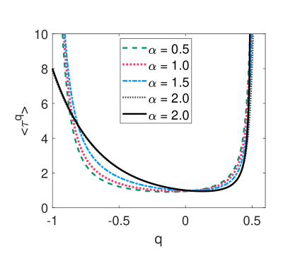
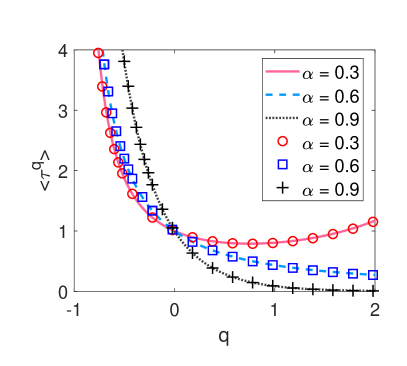
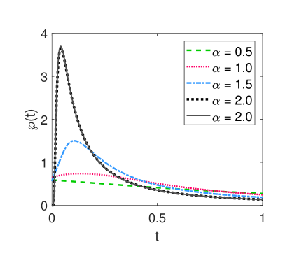
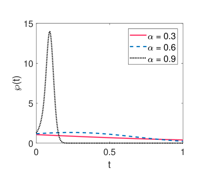
Figure 2: Top left: fractional order moments of the first-passage time PDF for symmetric ($0<\alpha\leq 2$, $\beta=0$) $\alpha$-stable laws in a semi-infinite domain with $d=0.5$. Here and in the following we set $K_{\alpha}=1$. Results are shown for the case when $L$ is sufficiently large (here we used $L=10^{12}$). Dashed lines represent the numerical solution of the space-fractional diffusion equation and the solid line shows the analytical result (48) for Brownian motion. Top right: fractional order moments of the first-passage time PDF for one-sided ($0<\alpha<1$, $\beta=1$) $\alpha$-stable laws in a semi-infinite domain. Symbols show the numerical solution of the space-fractional diffusion equation with $d=0.5$, $\Delta x=0.01$, and $\Delta t=0.001$, and lines represent the analytic result (56). Bottom left: first-passage time PDF of symmetric $\alpha$-stable laws with $0<\alpha\leq 2$ and $\beta=0$. Lines correspond to the numerical solution of the space-fractional diffusion equation and the solid line shows result (45). Bottom right: first-passage time PDF of one-sided ($0<\alpha<1$ with $\beta=1$) $\alpha$-stable laws obtained by numerical solution of the space-fractional diffusion equation.

5.2 Asymmetric LFs in a semi-infinite domain

5.2.1 One-sided $\alpha$-stable processes with $0<\alpha<1$ and $\beta=1$.

By applying the Skorokhod theorem, it can be shown that the first-passage time PDF of one-sided $\alpha$-stable laws has the exact form [48]

$$\wp(t)=\frac{\xi}{d^{\alpha}}M_{\alpha}\left(\frac{\xi t}{d^{\alpha}}\right)$$ (49)

with

$$\xi=\frac{K_{\alpha}}{\cos{(\alpha\pi(\rho-1/2))}},\,\,\,\rho=\frac{1}{2}+\frac{1}{\alpha\pi}\arctan{(\beta\tan{(\alpha\pi/2)})},$$ (50)

which connects to our case here via

$$\xi=\frac{K_{\alpha}}{\cos{(\alpha\pi/2)}},\,\,\,\rho=1.$$ (51)

Here $M_{\alpha}(z)$ is the Wright $M$-function [96, 124] (also sometimes called Mainardi function) with the integral representation [124] (page 241)

$$M_{\alpha}(z)=\frac{1}{2\pi i}\int\limits_{Ha}e^{\sigma-z\sigma^{\alpha}}\frac{\mathrm{d}\sigma}{\sigma^{1-\alpha}},\,\,\,z\in\mathbb{C},\,\,\,0<\alpha<1,$$ (52)

where the contour of integration Ha (the Hankel path) is the loop starting and ending at $-\infty$ and encircling the disk $|\sigma|\leq|z|^{1/\alpha}$ counterclockwise, i.e., $|\arg(\sigma)|\leq\pi$ on Ha. Here and below for the asymptotic behavior of the first-passage time PDFs we refer the reader to our recent paper [60]. The asymptotics of the $M$-function at short and long times is presented in appendix E of [60]. The long-time asymptotics of the PDF (49) is given by equations (31) and (32) of [60], while the short-time asymptotics of (49) is given by equation (33) of [60] (or equivalently, equation (71) below with $\rho=1$). By definition (25) of the moments of the first-passage time PDF and the first-passage time PDF (49) of one-sided stable laws, we find

$$\langle\tau^{q}\rangle = \int\limits_{0}^{\infty}t^{q}\frac{\xi}{d^{\alpha}}M_{\alpha}\left(\frac{\xi t}{d^{\alpha}}\right)\mathrm{d}t$$ (53)

$$= \frac{\xi}{d^{\alpha}}\int\limits_{0}^{\infty}t^{q}\frac{1}{2\pi i}\int\limits_{Ha}\sigma^{\alpha-1}\rme^{\sigma-\xi t(\sigma/d)^{\alpha}}\,\mathrm{d}\sigma\mathrm{d}t$$

$$= \frac{\xi}{d^{\alpha}}\frac{1}{2\pi i}\int\limits_{Ha}\sigma^{\alpha-1}\rme^{\sigma}\int\limits_{0}^{\infty}t^{q}\rme^{-\xi t(\sigma/d)^{\alpha}}\mathrm{d}t\mathrm{d}\sigma.$$

By change of variables $u=\xi t(\sigma/d)^{\alpha}$ in the inner integral and with the help of equation (47) we get

$$\langle\tau^{q}\rangle=\frac{d^{q\alpha}\Gamma(1+q)}{\xi^{q}}\frac{1}{2\pi i}\int\limits_{Ha}\sigma^{-q\alpha-1}\rme^{\sigma}\,\mathrm{d}\sigma.$$ (54)

Using Hankel’s contour integral

$$\frac{1}{\Gamma(z)}=\frac{1}{2\pi i}\int\limits_{Ha}\zeta^{-z}\rme^{\zeta}\mathrm{d}\zeta,\,\,\,z\in\mathbb{C},$$ (55)

we then obtain the fractional order moments of the first-passage time PDF for one-sided $\alpha$-stable laws with $0<\alpha<1$ and $\beta=1$,

$$\langle\tau^{q}\rangle=\frac{\Gamma(1+q)}{\Gamma(1+q\alpha)}\frac{d^{q\alpha}}{\xi^{q}},\,\,\,q>-1.$$ (56)

The MFPT ($q=1$) for one-sided $\alpha$-stable process was derived in [48, 68]. Also, from equation (27) and the Laplace transform of the first-passage time PDF, which has the form of the Mittag-Leffler function [48], it is possible to find all moments explicitly. In the right panel of figure 2 we show the results for the fractional order moments of one-sided $\alpha$-stable laws obtained by numerically solving the space-fractional diffusion equation, along with the analytical results of equation (56).

5.2.2 One-sided $\alpha$-stable processes with $0<\alpha<1$ and $\beta=-1$.

One-sided $\alpha$-stable laws with the stability index $0<\alpha<1$ and skewness parameter $\beta=-1$ satisfy the non-positivity of their increments. Therefore, the random walker never crosses the right boundary $d$. In the semi-infinite domain therefore the survival probability remains unity ($S(t)=1$) and the first-passage time PDF $\wp(t)=0$. Therefore, the fractional moments read

$$\langle\tau^{q}\rangle=\left\{\begin{array}[]{ll}0,&q<0\\ 1,&q=0\\ \infty,&q>0\end{array}\right..$$ (57)

Due to normalisation of the first-passage time PDF, $\langle\tau^{q}\rangle=1$ when $q=0$.

5.2.3 Extremal two-sided $\alpha$-stable processes with $1<\alpha<2$ and $\beta=-1$.

Stable laws with stability index $1<\alpha<2$ and skewness $\beta=1$ or $\beta=-1$ are called extremal two-sided skewed $\alpha$-stable laws [127]. Let us first consider the case $1<\alpha<2$, $\beta=-1$. By applying the Skorokhod theorem it can be shown that the first-passage time PDF of extremal two-sided $\alpha$-stable laws with $1<\alpha<2$ and $\beta=-1$ has the following exact form [60]

$$\wp(t)=\frac{t^{-1-1/\alpha}d}{\alpha\xi^{1/\alpha}}M_{1/\alpha}\left(\frac{d}{(\xi t)^{1/\alpha}}\right),$$ (58)

in terms of the Wright $M$-function $M_{1/\alpha}$. The long-time asymptotic of the PDF (58) is given by equation (41) of [60] or, equivalently, equation (68) below with $\rho=1/\alpha$. Respectively, the short-time asymptotic of equation (58) is given by equation (39) of [60], or by equation (71) below with $\rho=1/\alpha$.

For the considered case of extremal two-sided $\alpha$-stable laws with $1<\alpha<2$ and $\beta=-1$ by recalling the integral representation (52) of the $M$-function, the first-passage time PDF moments become

$$\langle\tau^{q}\rangle = \frac{d}{\alpha\xi^{1/\alpha}}\int\limits_{0}^{\infty}t^{q-1-1/\alpha}M_{1/\alpha}\left(\frac{d}{(\xi t)^{1/\alpha}}\right)\mathrm{d}t$$ (59)

$$= \frac{d}{\alpha\xi^{1/\alpha}}\int\limits_{0}^{\infty}t^{q-1-1/\alpha}\frac{1}{2\pi i}\int\limits_{Ha}\rme^{\sigma-d(\sigma/\xi t)^{1/\alpha}}\frac{\mathrm{d}\sigma}{\sigma^{1-1/\alpha}}\mathrm{d}t$$

$$= \frac{d}{\alpha\xi^{1/\alpha}}\frac{1}{2\pi i}\int\limits_{Ha}\sigma^{1/\alpha-1}\rme^{\sigma}\int\limits_{0}^{\infty}t^{q-1-1/\alpha}\rme^{-d(\sigma/\xi t)^{1/\alpha}}\mathrm{d}t\mathrm{d}\sigma.$$

Changing variables, $u=d(\sigma/\xi t)^{1/\alpha}$ in the inner integral and with the help of equation (47), we find

$$\langle\tau^{q}\rangle=\frac{d^{q\alpha}\Gamma(1-q\alpha)}{\xi^{q}}\frac{1}{2\pi i}\int\limits_{Ha}\sigma^{q-1}\rme^{\sigma}\mathrm{d}\sigma=\frac{\Gamma(1-q\alpha)}{\Gamma(1-q)}\frac{d^{q\alpha}}{\xi^{q}},\,\,\,-\infty<q<1/\alpha,$$ (60)

where in the last equality we used equation (55) to get the desired result. In the limit $\alpha=2$ we recover the fractional moments of the first-passage time PDF (48) for a Gaussian process. The left panel of figure 3 shows the results of equation (60) along with numerical solutions of the space-fractional diffusion equation. As can be seen the fractional order moments $-\infty<q<1/\alpha$ are finite, as they should.

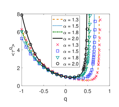
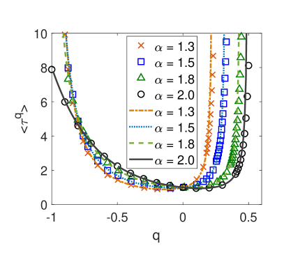
Figure 3: Left: Fractional order moments of the first-passage time PDF for extremal two-sided $\alpha$-stable laws in a semi-infinite domain with stability index $1<\alpha\leq 2$ and skewness $\beta=-1$. Symbols represent the numerical solution of the space-fractional diffusion equation and lines correspond to the analytic result (60). Right: same as in the left panel but with skewness $\beta=1$. Lines show results of equation (67). In both panels, we used $d=0.5$ and $L=10^{12}$.

5.2.4 Extremal two-sided $\alpha$-stable processes with $1<\alpha<2$ and $\beta=1$.

Applying the Skorokhod theorem it can be shown that the first-passage time PDF of the extremal two-sided $\alpha$-stable law with stability index $1<\alpha<2$ and skewness $\beta=1$ has the following series representation [60] (see equation (D.73))

$$\wp(t)=\frac{t^{-2+1/\alpha}d^{\alpha-1}}{\alpha\xi^{1-1/\alpha}}\sum_{n=0}^{\infty}\frac{(d^{\alpha}/{\xi t})^{n}}{\Gamma{(\alpha n+\alpha-1)}\Gamma{(-n+1/\alpha)}}.$$ (61)

Now, with the help of Euler’s reflection formula $\Gamma(1-z)\Gamma(z)\sin{(\pi z)}=\pi$ and the relation $\sin{\pi(z-n)}=(-1)^{n}\sin{(\pi z)}$ we rewrite this expression in the form

$$\wp(t)=\frac{\sin{(\pi/\alpha)}t^{-2+1/\alpha}d^{\alpha-1}}{\pi\alpha\xi^{1-1/\alpha}}\sum_{n=0}^{\infty}\frac{\Gamma{(n+1-1/\alpha)}(-d^{\alpha}/{\xi t})^{n}}{\Gamma{(\alpha n+\alpha-1)}}.$$ (62)

To obtain the long-time asymptotics of the PDF we take $n=0$ in equation (62) and arrive at the power-law decay given by equation (43) of [60] or, equivalently, equation (68) below with $\rho=1-1/\alpha$.

To calculate the moments of the first-passage time we use the relation between the Wright generalised hypergeometric function and the $H$-function [125] (see equations (1.123) and (1.140)). We arrive at

$$\wp(t)=\frac{\sin{(\pi/\alpha)}t^{-2+1/\alpha}d^{\alpha-1}}{\pi\alpha\xi^{1-1/\alpha}}H_{2,2}^{1,2}\left[\frac{d^{\alpha}}{\xi t}\left|\begin{array}[]{l}(0,1),(1/\alpha,1)\\ (0,1),(2-\alpha,\alpha)\end{array}\right.\right].$$ (63)

Further, with the help of the inversion property of the $H$-function [125] (Property 1.3, equation (1.58)), we have

$$\wp(t)=\frac{\sin{(\pi/\alpha)}t^{-2+1/\alpha}d^{\alpha-1}}{\pi\alpha\xi^{1-1/\alpha}}H_{2,2}^{2,1}\left[\frac{\xi t}{d^{\alpha}}\left|\begin{array}[]{l}(1,1),(\alpha-1,\alpha)\\ (1,1),(1-1/\alpha,1)\end{array}\right.\right].$$ (64)

At short times the $H$-function representation of the first-passage PDF leads to equation (44) of [60] or, equivalently, equation (71) below with $\rho=1-1/\alpha$. Substitution of equation (64) into (25) yields

$$\langle\tau^{q}\rangle=\int\limits_{0}^{\infty}\frac{\sin{(\pi/\alpha)}t^{q-2+1/\alpha}d^{\alpha-1}}{\pi\alpha\xi^{1-1/\alpha}}H_{2,2}^{2,1}\left[\frac{\xi t}{d^{\alpha}}\left|\begin{array}[]{l}(1,1),(\alpha-1,\alpha)\\ (1,1),(1-1/\alpha,1)\end{array}\right.\right]\mathrm{d}t.$$ (65)

Recalling the Mellin transform of the $H$-function [125] (page 47, equation (2.8)), we find

$$\langle\tau^{q}\rangle=\frac{\sin{(\pi/\alpha)}\Gamma(1-1/\alpha-q)\Gamma(q+1/\alpha)\Gamma{(q)}}{\pi\alpha\Gamma(q\alpha)}\frac{d^{q\alpha}}{\xi^{q}}.$$ (66)

Using Euler’s reflection formula $\Gamma(1-z)\Gamma(z)\sin{(\pi z)}=\pi$, we finally get

$$\langle\tau^{q}\rangle=\frac{\sin{(\pi/\alpha)}}{\sin{(\pi(q+1/\alpha))}}\frac{\Gamma(1+q)}{\Gamma(1+q\alpha)}\frac{d^{q\alpha}}{\xi^{q}},\,\,\,-1<q<1-1/\alpha,$$ (67)

where $\xi$ is given by equation (50). The same result with a different method was given in dimensionless form in [126] (see proposition 4). For $\alpha=2$, we again consistently recover result (48). In the right panel of figure 3 we plot the numerical result for the space-fractional diffusion equation and the analytic result corresponding to equation (67). As expected, moments of order $-1<q<1-1/\alpha$ are finite.

For completeness in figure 4 we also provide a comparison of the first-passage time PDFs for the extremal two-sided $\alpha$-stable processes in the semi-infinite domain with $\beta=-1$ and $\beta=1$. One can see (left panel) that in the limit $t\to 0$ the first-passage time PDF tends to zero for $\beta=-1$ and attains a finite value for $\beta=1$. Respectively, in the long-time limit (right panel) the PDFs decay differently, faster for $\beta=-1$ (like $\simeq t^{-1-1/\alpha}$) and slower for $\beta=1$ (like $\simeq t^{-2+1/\alpha}$).

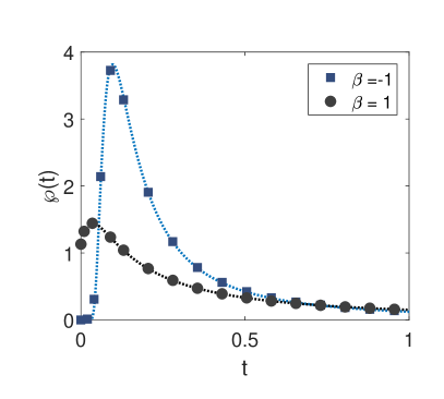
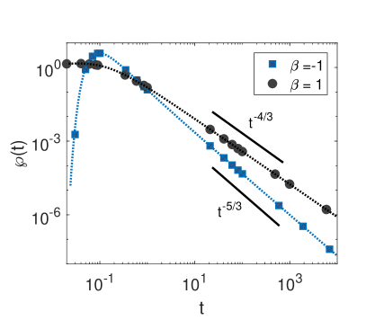
Figure 4: Left: first-passage time PDF at short times for the extremal $\alpha$-stable processes in the semi-infinite domain with stability index $\alpha=1.5$. Right: long-time behaviour of the same PDF on log-log. The black lines show the asymptotic behaviour of the PDFs. In both panels $d=0.5$, symbols represent the numerical solution of the space-fractional diffusion equation, and the dotted lines show the analytical results namely, equation (58) for $\beta=-1$ and equation (61) for $\beta=1$.

5.2.5 General asymmetric form of $\alpha$-stable processes

In this section we present the first-passage properties of $\alpha$-stable processes in general form. By applying the Skorokhod theorem for $\alpha\in(0,1)$ with $\beta\in(-1,1)$, for $\alpha=1$ with $\beta=0$, as well as for $\alpha\in(1,2]$ with $\beta\in[-1,1]$, it was shown that the first-passage time PDF has the following power-law decay [60]

$$\wp(t)\sim\frac{\rho(K_{\alpha}(1+\beta^{2}\tan^{2}{(\alpha\pi/2)})^{1/2})^{-\rho}d^{\alpha\rho}}{\Gamma(1-\rho)\Gamma(1+\alpha\rho)}t^{-\rho-1}=\frac{1}{\alpha\Gamma(1-\rho)\Gamma(\alpha\rho)}\frac{d^{\alpha\rho}}{\xi^{\rho}}t^{-\rho-1},$$ (68)

where $\xi$ and $\rho$ are defined in equation (50). It is obvious that the corresponding integral (25) is finite for moments $q<\rho$, otherwise the integral diverges. To estimate the behaviour of the first-passage time PDF at short times, we employ the asymptotic expression of LFs for large $x$. For the purpose of this derivation, we follow the method introduced in [123] and assume that the starting position is at $x_{0}=0$ while the boundary is located at $x=d$, which is identical to our setting in a semi-infinite domain. Therefore, the survival probability at short times reads

$$S(t|0)=\int\limits_{-\infty}^{d}P_{\alpha,\beta}(x,t|0)\mathrm{d}x=1-\int\limits_{d}^{\infty}P_{\alpha,\beta}(x,t|0)\mathrm{d}x,$$ (69)

where the $\alpha$-stable law with the stability index $\alpha\in(0,2]$ ($\alpha\neq 1$) and skewness $\beta\in(-1,1]$ in the limit $x\to\infty$ is given by [127]

$$P_{\alpha,\beta}(x,t|0) \sim \pi^{-1}(1+\beta^{2}\tan^{2}{(\alpha\pi/2)})^{1/2}\sin{(\alpha\pi\rho)}\Gamma(1+\alpha)\frac{K_{\alpha}t}{x^{1+\alpha}}$$ (70)

$$= \pi^{-1}\sin(\alpha\pi\rho)\Gamma(1+\alpha)\frac{\xi t}{x^{1+\alpha}}.$$

By substitution into equation (69) and recalling equation (23) we arrive at

$$\wp(t\to 0)=\pi^{-1}\sin(\alpha\pi\rho)\Gamma(\alpha)\frac{\xi}{d^{\alpha}}.$$ (71)

It is easy to check with the use of equation (50) that the first-passage time PDF is only zero for Brownian motion ($\alpha=2$ and $\rho=1/2$) at short times. Otherwise, the boundary is crossed immediately with a finite probability on the first jump. To support our conclusion regarding the existence of fractional order moments of the first-passage time PDF for general asymmetric form of the $\alpha$-stable law, we plot the fractional order moments and the first-passage time PDF for two sets of the skewness, $\beta=0.5$ and $-0.5$, and different values of the stability index $\alpha$. The results are shown in figure 5, and it can be seen moments with $-1<q<\rho$ are finite. The lower bound ($-1<q$), arising due to the finite jump in the first-passage time PDF at $t\to 0$, can be seen in the bottom panels of figure 5. Similar to the symmetric case with $\beta=0$ shown in figure 2 the values of the first-passage time PDF at $t\to 0$ obtained by numerical solution of the space-fractional diffusion equation are in perfect agreement with the behaviour provided by equation (71). We also note that in [75] (theorem 2) presented a sufficient condition for the finiteness of the moments of the first-passage time of the general Lévy process which is in agreement with our results for LFs in general asymmetric form.

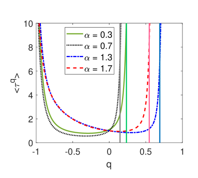
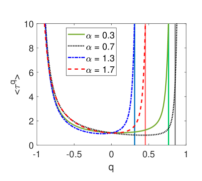
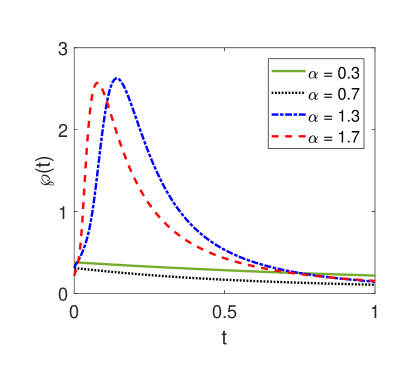
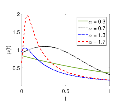
Figure 5: Left: fractional order moments of the first-passage time PDF (top) and the first-passage time PDF (bottom) of $\alpha$-stable laws in the semi-infinite domain with skewness $\beta=-0.5$. Right: the same but for skewness $\beta=0.5$. For all panels we used $d=0.5$ and $L=10^{12}$. The lines represent numerical solutions of the space-fractional diffusion equation and vertical lines in the top panels represent the limit $q=\rho$.

6 First passage time properties of LFs in a bounded domain

In this section we consider an LF in the interval $[-L,L]$ with initial point $x_{0}$ and absorbing boundary conditions at both interval borders (figure 1). Eventually, the LF is absorbed, and our basic goal is to characterise the time dependence of this trapping phenomenon. From equation (34) and with the space-fractional operators (5) and (6) we find

$$K_{\alpha}\left(\frac{R_{\alpha,\beta}}{\Gamma(n-\alpha)}\int\limits_{-L}^{x_{0}}\frac{\langle\tau\rangle^{(n)}(\zeta)}{(x_{0}-\zeta)^{\alpha-n+1}}\,\mathrm{d}\zeta+\frac{L_{\alpha,\beta}(-1)^{n}}{\Gamma(n-\alpha)}\int\limits_{x_{0}}^{L}\frac{\langle\tau\rangle^{(n)}(\zeta)}{(\zeta-x_{0})^{\alpha-n+1}}\,\mathrm{d}\zeta\right)=-1.$$ (72)

Applying the boundary condition $\langle\tau\rangle(\pm L)=0$ and the fact that ${}_{0}D_{L\pm x_{0}}^{\alpha}(L\pm x_{0})^{\alpha-n+1}=const$ [99] (page 626, theorem 30.7) leads us to a solution of equation (72) in the following form

$$\langle\tau\rangle(x_{0})=C_{\alpha,\beta}(L-x_{0})^{\mu}(L+x_{0})^{\nu},$$ (73)

where $C_{\alpha,\beta}$ is a normalisation factor. First we consider the case $0<\alpha<1$ ($n=1$). After substitution of equation (73) into (72) and some calculations (see details in B) we obtain

$$\mu=\alpha\rho,\,\,\,\nu=\alpha-\alpha\rho$$ (74)

and

$$C_{\alpha,\beta}=\frac{\cos{(\alpha\pi(\rho-1/2))}}{\Gamma(1+\alpha)K_{\alpha}}=\frac{1}{\Gamma(1+\alpha)\xi}.$$ (75)

For the case $1<\alpha\leq 2$ ($n=2$) a similar procedure leads to the same result, and formulas (74) and (75) are valid for all $\alpha\in(0,2]$ with $\beta\in[-1,1]$ (excluding the case $\alpha=1$, $\beta\neq 0$). Finally, the MFPT for LFs in a bounded domain $[-L,L]$ reads

$$\langle\tau\rangle=\frac{(L-x_{0})^{\alpha\rho}(L+x_{0})^{\alpha-\alpha\rho}}{\Gamma(1+\alpha)\xi},$$ (76)

where $\rho$ and $\xi$ are given in expression (50). We note that in [77] from the Green’s function of a Lévy stable process [78] the MFPT of LFs in the interval (-1, 1) in the dimensionless Z-form of the characteristic function ($K_{\alpha}^{Z}=1$) is given (see Remark 5 in [77]). To see the equivalence between equation (76) and the result in [77] we note that the following relation between the parameters in the A- and Z-forms is established and reads (see equation (A.11) in [60])

$$\rho=\frac{1}{2}+\frac{1}{\alpha\pi}\arctan\left(\beta_{A}\tan\left(\frac{\alpha\pi}{2}\right)\right),\quad K_{\alpha}^{Z}=\frac{K_{\alpha}^{A}}{\cos{(\alpha\pi(\rho-1/2))}}.$$ (77)

Here, we use the standard A-from parameterisation for the characteristic function.

6.1 Symmetric $\alpha$-stable processes

For symmetric $\alpha$-stable processes in a bounded domain, the MFPT for stability index $0<\alpha\leq 2$ and $|x_{0}|<L$ in $N$-dimension is given by [65]

$$\langle\tau\rangle=K(\alpha,N)(L^{2}-x_{0}^{2})^{\alpha/2},$$ (78)

where

$$K(\alpha,N)=\Gamma\left(\frac{N}{2}\right)\left[2^{\alpha}\Gamma\left(1+\frac{\alpha}{2}\right)\Gamma\left(\frac{N+\alpha}{2}\right)\right]^{-1}.$$ (79)

In one dimension by using the duplication rule $2^{2z}\Gamma(z)\Gamma(z+1/2)=2\sqrt{\pi}\Gamma(2z)$ this equation reads [80, 83]

$$\langle\tau\rangle=\frac{(L^{2}-x_{0}^{2})^{\alpha/2}}{\Gamma(1+\alpha)}.$$ (80)

For the setup in figure 1, $x_{0}=L-d$ and by defining $l=d/L$, in dimensional variables the MFPT yields in the form

$$\langle\tau\rangle=\frac{(d(2L-d))^{\alpha/2}}{\Gamma(1+\alpha)K_{\alpha}}=\frac{L^{\alpha}(l(2-l))^{\alpha/2}}{\Gamma(1+\alpha)K_{\alpha}}.$$ (81)

This result is consistently recovered from the general formula (76) by setting $\rho=1/2$ (or, equivalently, $\beta=0$).

The second moment of the first-passage time PDF for symmetric $\alpha$-stable process with stability index $0<\alpha\leq 2$ and $|x_{0}|<L$ in $N$ dimensions was derived in [65],

$$\langle\tau^{2}\rangle=\alpha L^{\alpha}K(\alpha,N)^{2}\int\limits_{x_{0}^{2}}^{L^{2}}\left(s-x_{0}^{2}\right)^{\alpha/2-1}F\left(-\frac{\alpha}{2};\frac{N}{2};\frac{N+\alpha}{2};sL^{-2}\right)\mathrm{d}s,$$ (82)

where $F$ is the Gauss hypergeometric function defined in equation (110). Analogous to the MFPT we set $N=1$, $x_{0}=L-d$, and in order to make time dimensional, equation (82) has to be divided by $K_{\alpha}^{2}$. Equation (82) is reduced to a simple form for Brownian motion only [43],

$$\langle\tau^{2}\rangle=\frac{L^{4}}{12K_{\alpha}^{2}}(l^{2}-2l)(l^{2}-2l-4),$$ (83)

where $l=d/L$. The behaviour of arbitrary-order moments is similar and reads $\langle\tau^{m}\rangle\propto L^{m\alpha}/K_{\alpha}^{m}$ (see figure 9), for the case when we start the process at the centre of the interval $[-L,L]$.

In figure 6 we study the MFPT for symmetric $\alpha$-stable processes with varying initial position. We employ two different interval lengths and plot the MFPT versus $d$ for different sets of the stability index $\alpha$. As can be seen, for interval length of $L=0.7$, regardless of the starting point of the random walker the MFPT is always longer for smaller $\alpha$. In contrast, for interval length $L=2.5$, when the starting point of the random walker is close to the centre of the interval, for larger $\alpha$ the MFPT is longer. When the starting point gets closer to the boundaries, the behaviour is opposite. These observations are in line with the fact that LFs have a propensity for long but rarer jumps, a phenomenon becoming increasingly pronounced when the value of $\alpha$ decreases. Conversely, LFs have short relocation events with a higher frequency for values $\alpha$ close to 2. Therefore, for small intervals (left panel of figure 6) it is easier to cross the boundaries when short relocation events happen with a high frequency, corresponding to Lévy motion with $\alpha$ closer to 2. In the opposite case, LFs with low-frequency large jumps ($\alpha\to 0$) can escape more efficiently from large intervals (right panel of figure 6), except for initial positions close to the boundaries. We also note that in both panels of figure 6, when the stability index $\alpha$ gets closer to $0$, the MFPT becomes flatter away from the boundaries. This result implies that with different starting points the random walker crosses the interval by a single jump—concurrently, the MFPT has a small variation.

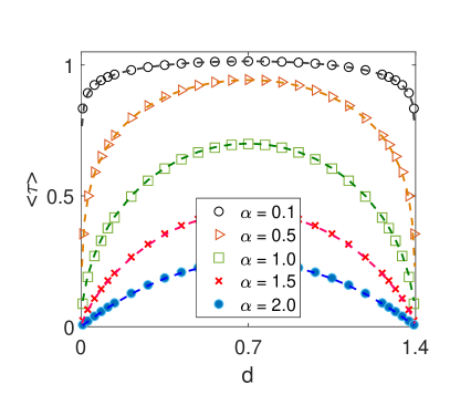
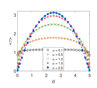
Figure 6: MFPT versus distance $d$ of the initial point of the random process from the right side boundary for symmetric $\alpha$-stable processes ($\beta=0$) and different sets of the stability index $\alpha$. Left: $L=0.7$. Right: $L=2.5$. Dashed lines show the analytic solution (81) and symbols represent numerical solutions of the space-fractional diffusion equation.

6.2 Asymmetric $\alpha$-stable processes

6.2.1 One-sided $\alpha$-stable processes with $0<\alpha<1$ and $\beta=1$.

This type of jump length distribution is defined on the positive axis. Therefore the situation for this process in semi-infinite and bounded domains is similar and moments for the first-passage time PDF turn out to be exactly the same as in equation (56) obtained above. Another method to find the moments of the first-passage time PDF is to employ relation (43), addressed originally in [83] for symmetric $\alpha$-stable laws. The space-fractional operator for one-sided $\alpha$-stable laws ($0<\alpha<1$ and $\beta=1$) reads

$$D_{x_{0}}^{\alpha}=-\frac{1}{\cos{(\alpha\pi/2)}}\,_{x_{0}}D_{L}^{\alpha}.$$ (84)

We apply the space-fractional integration operator $D_{x_{0}}^{-m\alpha}$ on both sides of equation (43) and get (see C for details)

$$\langle\tau^{m}\rangle(x_{0})=\,_{x_{0}}D_{L}^{-m\alpha}{\frac{\cos^{m}{(\alpha\pi/2)}\Gamma(1+m)}{{K_{\alpha}}^{m}}},$$ (85)

where the sequential rule was used, namely, $(D^{\alpha}_{x_{0}})^{m}=D^{m\alpha}_{x_{0}}$ [96] (page 86, equation (2.169)). The space-fractional integration operator ${}_{x_{0}}D_{L}^{-m\alpha}$ used here is defined as [96] (page 51, equation (2.40))

$$_{x_{0}}D_{L}^{-m\alpha}{f(x)}=\frac{1}{\Gamma(m\alpha)}\int\limits_{x_{0}}^{L}\frac{f(\zeta)}{(\zeta-x_{0})^{1-m\alpha}}\,\mathrm{d}\zeta.$$ (86)

By substitution of equation (86) with $f(\zeta)={\bf 1}$ into equation (85) we arrive at

$$\langle\tau^{m}\rangle(x_{0})=\frac{\cos^{m}{(\alpha\pi/2)}\Gamma(1+m)}{\Gamma(m\alpha){K_{\alpha}}^{m}}\int\limits_{x_{0}}^{L}(\zeta-x_{0})^{m\alpha-1}\mathrm{d}\zeta=\frac{\Gamma(1+m)}{\Gamma(1+m\alpha)}\frac{d^{m\alpha}}{\xi^{m}}.$$ (87)

This result is the same as equation (56) with parameter $\xi$ defined in (50) and $d=L-x_{0}$. The same result for $m=1$ is also shown in [48, 68]. Moreover from equation (76) by setting $\rho=1$ or $\beta=1$ ($0<\alpha<1$) we arrive at above expression with $m=1$. The left panels of figure 7 show the MFPT of one-sided LFs ($0<\alpha<1$ and $\beta=1$) for different values of the stability index $\alpha$ for two interval lengths (top: $L=0.7$, bottom: $L=2.5$). For interval length $L=0.7$, smaller $\alpha$ values lead to longer MFPTs for different initial positions, except for the situations when the LF starts really close to the left boundary. This observation is due to the lower frequency of long-range jumps compared to high-frequency shorter-range jumps for larger $\alpha$ values, similar to the above. For interval length $L=2.5$, when the initial position of the random walker is located a distance $d<2$ away from the right boundary, for smaller $\alpha$ it takes longer to cross the right boundary. For larger $d$ values the smaller $\alpha$ values overtake the LFs with the intermediate stable index $\alpha=0.5$. Note, however, that the MFPT for $\alpha=0.9$ remains shorter than for LFs with the smaller stable index. For increasing interval length low-frequency long jumps will eventually win out unless the particle is released close to an absorbing boundary, compare also the discussion in [19, 20]. Thus, the crossing of curves with different $\alpha$ values in the left panel of figure 7 has a simple physical meaning: it reflects the growing role of long jumps with smaller $\alpha$ when the distance $d$ to the right boundary (respectively, the interval length $L$) increases.

6.2.2 One-sided $\alpha$-stable processes, $0<\alpha<1$, $\beta=-1$.

For one-sided $\alpha$-stable processes with $0<\alpha<1$ and $\beta=-1$ the space-fractional operator reads

$$D_{x_{0}}^{\alpha}=-\frac{1}{\cos{(\alpha\pi/2)}}\,_{-L}D_{x_{0}}^{\alpha},$$ (88)

and following a similar procedure as for the case $0<\alpha<1$ with $\beta=1$, we obtain

$$\langle\tau^{m}\rangle(x_{0})=\frac{\cos^{m}{(\alpha\pi/2)}\Gamma(1+m)}{\Gamma(m\alpha){K_{\alpha}}^{m}}\int\limits_{-L}^{x_{0}}(\zeta-x_{0})^{m\alpha-1}\mathrm{d}\zeta=\frac{(2L-d)^{m\alpha}}{\xi^{m}}\frac{\Gamma(1+m)}{\Gamma(1+m\alpha)}.$$ (89)

By setting $\rho=0$ or $\beta=-1$ ($0<\alpha<1$) for $m=1$ we recover the same result as in equation (76). The behaviour of the MFPT for this section is similar to the left panels of figure 7, apart from substituting $d$ for $2L-d$.

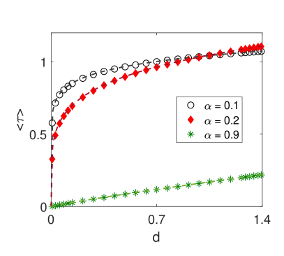
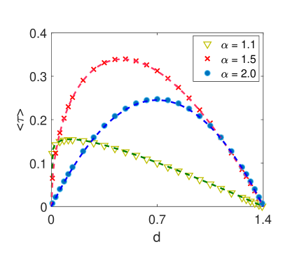
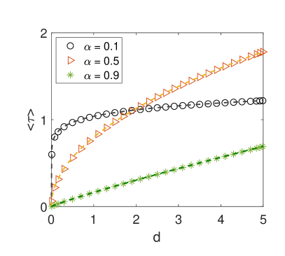
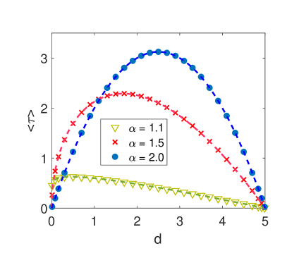
Figure 7: MFPT versus distance $d$ of the initial position of the LF from the right boundary. Top panels: interval length $L=0.7$. Bottom panels: interval length $L=2.5$. Left panels: extremal one-sided $\alpha$-stable processes with $\beta=1$ and different sets of the stability index $\alpha$. Dashed lines represent the analytic result (87) while symbols represent the numerical solution of the space-fractional diffusion equation. Right panels: MFPT for extremal two-sided $\alpha$-stable processes with skewness $\beta=1$. Dashed lines show the analytic result (91) and symbols represent the numerical solution of the space-fractional diffusion equation.

6.2.3 Extremal two-sided $\alpha$-stable processes with $1<\alpha<2$ and $\beta=-1,1$.

For extremal two-sided $\alpha$-stable processes with stability index $1<\alpha<2$, when the initial position is the distance $d$ away from the right boundary and for skewness $\beta=-1$ (or $\rho=1/\alpha$) in (76) we obtain the MFPT

$$\langle\tau\rangle=\frac{d(2L-d)^{\alpha-1}}{\Gamma(1+\alpha)\xi},$$ (90)

where $\xi$ defied in equation (50). For the case $\beta=1$, by setting $\rho=1-1/\alpha$ in equation (76) the following result yields,

$$\langle\tau\rangle=\frac{d^{\alpha-1}(2L-d)}{\Gamma(1+\alpha)\xi}.$$ (91)

In contrast to the completely one-sided cases above, in results (90) and (91) two factors appear that include the distances $d$ and $2L-d$. As a direct consequence, we recognise the completely different functional behaviour in the right panels of figure 7. Namely, the MFPT decays to zero at both interval boundaries.

For completely asymmetric LFs the first-passage of the two-sided exit problem was addressed in [68, 69, 70, 71, 72, 73]. A different expression (instead of $d^{\alpha-1}$ in equation (91) it is $d^{\alpha}$) for the MFPT of completely asymmetric LFs with $1<\alpha<2$ and $\beta=1$ in dimensionless form was derived with the help of the Green’s function method in [68] (see equation (1.8)). In [71] the distribution of the first-exit time from a finite interval for extremal two-sided $\alpha$-stable probability laws with $1<\alpha<2$ and $\beta=-1$ was reported in the Laplace domain.

In the right panels of figure 7 we show the MFPT for extremal $\alpha$-stable processes with skewness $\beta=1$ for two different interval lengths as function of the initial distance $d$ from the right boundary. To compare the MFPT of extremal two-sided LFs with arbitrary $\alpha\in(1,2)$ and $\beta=1$ with that of Brownian motion, we employ equation (91) and obtain

$$\langle\tau\rangle|_{\alpha=2}-\langle\tau\rangle|_{\alpha}=0,$$ (92)

with $\xi$ defined in equation (50). By solving for $d$, we find

$$d=\left(\frac{2\cos{(\alpha\pi(1/2-1/\alpha))}}{\Gamma(1+\alpha)}\right)^{1/(2-\alpha)}.$$ (93)

For $\alpha=1.1$ and $\alpha=1.5$ the MFPT is equal with the Brownian case for $d=0.261$ and $d=1.132$, respectively. The right side panels of figure 7 indeed demonstrate that as long as the distance $d$ of the initial position of the LF is within the range $0<d<0.261$ from the right boundary for $\alpha=1.1$ and in the range $0<d<1.132$ for $\alpha=1.5$, Brownian motion has a shorter MFPT, otherwise the LF is faster. In general, if $d$ is less than the term on the right hand side of equation (93) for arbitrary $\alpha\in(1,2)$, Brownian motion is faster on average. In the opposite case, long-range relocation events and left direction effective drift of LFs with positive skewness parameter lead to shorter MFPTs.

6.2.4 General asymmetric $\alpha$-stable processes

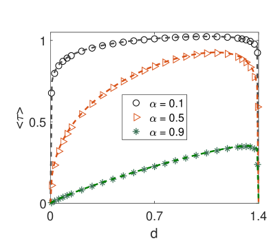
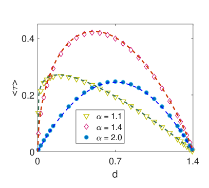
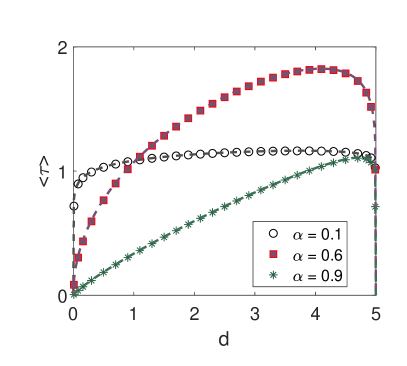
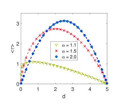
Figure 8: Left: MFPT of a general asymmetric $\alpha$-stable process versus initial distance $d$ from the right boundary for skewness $\beta=0.5$ and $\alpha\in(0,1)$. Right: the same for $\alpha\in(1,2)$. Top: interval length $L=0.7$. Bottom: interval length $L=2.5$. Symbols are numerical solutions of the space-fractional diffusion equation, the dashed lines represent equation (95).

We finally show the result for the first-passage time moments of asymmetric $\alpha$-stable processes with arbitrary skewness $\beta$. The corresponding result for the MFPT with $\alpha\in(0,2]$ and $\beta\in[-1,1]$ (excluding the case $\alpha=1$ and $\beta\neq 0$) has the following expression

$$\langle\tau\rangle=\frac{(L-x_{0})^{\alpha\rho}(L+x_{0})^{\alpha-\alpha\rho}}{\Gamma(1+\alpha)\xi}.$$ (94)

Setting $d=L-x_{0}$ and $2L-d=L+x_{0}$ we find

$$\langle\tau\rangle=\frac{d^{\alpha\rho}(2L-d)^{\alpha-\alpha\rho}}{\Gamma(1+\alpha)\xi}$$ (95)

with $\rho$ and $\xi$ defined in equation (50). In figure 8, analogous to figure 7, we show the MFPT for $\alpha$-stable processes with skewness $\beta=0.5$ and two different interval lengths ($L=0.7$ and $L=2.5$). The left panels of figure 8 show the MFPT versus the distance $d$ from the right boundary for $\alpha$-stable processes with $0<\alpha<1$ and skewness $\beta=0.5$, for the two different lengths. As can be seen for the smaller interval, increasing $\alpha$ from $0.1$ to $0.9$, regardless of the initial position the MFPT decreases. This result can be explained as follows. An $\alpha$-stable process with stability index $0<\alpha<1$ and skewness $\beta=0.5$, has a longer tail on the positive axis and a shorter tail on the negative axis. Moreover, with increasing $\alpha$ from $0.1$ to $0.9$, the process experiences a larger effective drift to the right boundary. Concurrently, when $\alpha$ decreases (increases), larger (shorter) jumps are possible with lower (higher) frequency. Therefore, with increasing $\alpha$ the possibility of shorter jumps with higher frequency and a larger effective drift toward the right side absorbing boundary arises and leads to shorter MFPTs. The decay of the MFPT around $d=1.4$, when the initial position is close to the left boundary, shows us the effect of small jumps of the negative short tail of the underlying $\alpha$-stable law. The behaviour of the MFPT in the larger interval is more complicated. For initial positions with distance $d<1$ from the right boundary increasing $\alpha$ leads to decreasing MFPTs. This is due to the dominance of an effective drift to the right and a higher frequency of long jumps when $\alpha$ changes from $0.1$ to $0.9$. Conversely, when $d>1$ we observe two scenarios. First, for $0.1<\alpha<0.6$, with increasing $\alpha$ MFPT increases. We can explain this result as follows. By increasing $\alpha$ in the range $(0.1,0.6)$ the long relocation events dominate the effective drift and higher frequency events with shorter jump length. Second, for $0.6<\alpha<0.9$, with increasing $\alpha$ the MFPT decreases. This is now due to the dominance of the effective drift and higher frequency of shorter jump events against long-range jumps in the range $0.6<\alpha<0.9$.

$\alpha$-stable processes with $1<\alpha<2$ and $\beta=0.5$, have a heavier tail on the positive axis and a resulting effective drift to the left. Based on the above properties, the behaviour of MFPT is quite rich, as can be seen in the right panels of figure 8. For instance, for interval length $L=0.7$, when $\alpha\in(1.4,2)$, regardless of the initial position, Brownian motion always has a shorter MFPT, whereas for $\alpha\in(1,1.4)$ it does depends on the initial position. For the interval length $L=2.5$, when the initial position is located in $2.5<d<5$, smaller $\alpha$ always has a shorter MFPT. Otherwise, the superiority of LFs over the Brownian particle depends on its initial position.

When the initial point of the random process is kept at the centre of the interval ($x_{0}=0$), we show results for the MFPT and higher moments of the first-passage time PDF for different stability $\alpha$ as function of the interval length for symmetric and asymmetric $\alpha$-stable processes in figure 9. As can be seen, the moments of the first-passage time PDF scale like $\langle\tau^{m}\rangle\sim L^{m\alpha}/K_{\alpha}^{m}$ independent of the skewness $\beta$.

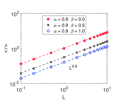
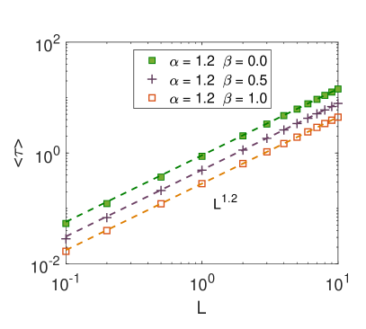
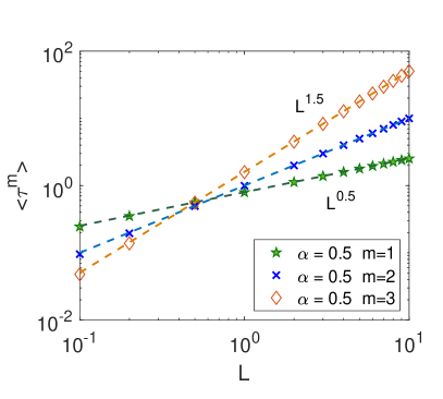
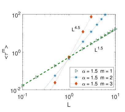
Figure 9: Top: MFPT versus interval length $L$ when the initial point is in the centre of the interval ($d=L$) for different values of the skewness $\beta$ in log-log scale. Symbols show numerical solutions of the space-fractional diffusion equation and dashed lines represent equation (95). Bottom: higher order moments of the first-passage time PDF versus interval length $L$ for $\beta=1$ and two values of the stability index $\alpha$ in log-log scale. Symbols show the numerical solutions of the space-fractional diffusion equation and dashed lines are equations (56) and (91).

6.3 Further properties of the MFPT

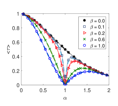
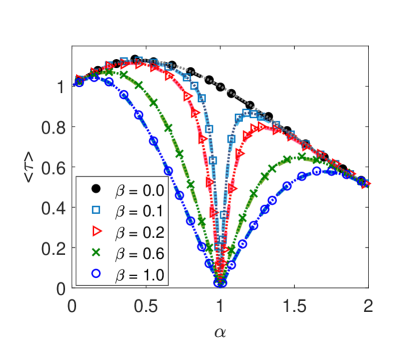
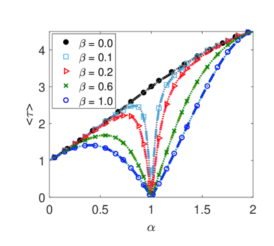
Figure 10: MFPT of an asymmetric $\alpha$-stable process for $L=0.5$ (top left), $L=1.0$ (top right), and $L=3$ (bottom) versus $\alpha$ when the initial position is in the centre of the interval ($d=L$ in figure 1). Symbols show results of Langevin equation simulations, dashed lines are based on the numerical solution of the space-fractional diffusion equation, and the dotted lines show the analytic solution (95).

In this section, we study the MFPT versus the index of stability $\alpha$. In figure 10 we fix the initial position of the random process to the centre of the interval ($d=L$ in figure 1) and plot the MFPT versus the stability index $\alpha$ for different skewness $\beta$, for three different interval lengths $L$. As can be seen, there is a perfect agreement between the results based on the space-fractional diffusion equation and the Langevin dynamic approach with the analytic result (95). To elucidate the behaviour of the MFPT in figure 10 we remind the reader of some properties of $\alpha$-stable laws. First, $\alpha$-stable laws with smaller $\alpha$ have a heavier tail and the associated frequency of long-range relocation events is smaller compared to laws with larger $\alpha$, for which short jumps with higher frequency are dominant. Second, symmetric $\alpha$-stable probability laws have the same tail on both sides. Third, $\alpha$-stable laws with $0<\alpha<1$ and skewness $\beta>0$ have an effective drift to the right and a longer tail on the positive axis. Moreover, when $\alpha\to 1_{-}$ with $\beta>0$, the effective drift to the right direction increases. Conversely, $\alpha$-stable laws with $1<\alpha<2$ and skewness $\beta>0$ have an effective drift to the left and a longer tail on the positive axis (see the bottom panel of figure 3 in [60]). When $\alpha\to 1_{+}$ with $\beta>0$, the effective drift to the left increases.

For a small interval length ($L=0.5$, top left panel of figure 10), short relocation events with higher frequency (larger $\alpha$) of symmetric LFs cross the boundaries quite quickly (full black circles), whereas in large intervals ($L=3$, bottom panel of figure 10), long-range relocation events of symmetric LFs lead to shorter MFPTs (full black circles). For intermediate interval length ($L=1$, top right panel in figure 10), by increasing $\alpha$ from $0$ to $\approx 0.46$ the MFPT increases, but for $\alpha\in(0.46,2]$ this behaviour reverts. This observation is due to the tipping balance between long jumps with low frequency and short jumps with high frequency for $\alpha$ less and larger than $0.46$, respectively.

Conversely, as can be seen from all panels in figure 10, on converging to the limit $\alpha\to 1$ from both sides with skewness $\beta\neq 0$, the MFPT tends to zero, which is in agreement with the analytical result (95). To explain this phenomenon we follow [31, 33] and first rewrite the characteristic function (1) and (2) of the LFs as

$$\ell_{\alpha,\beta}(k,t)=\exp\left(K_{\alpha}t\left[-|k|^{\alpha}+ik\omega(k,\alpha,\beta)\right]+i\mu kt\right),$$ (96)

where

$$\omega(k,\alpha,\beta)=\left\{\begin{array}[]{ll}|k|^{\alpha-1}\beta\tan(\pi\alpha/2),&\alpha\neq 1\\ -(2/\pi)\beta\ln|k|,&\alpha=1\end{array}\right..$$ (97)

The function $\omega(k,\alpha,\beta)$ is not continuous at $\alpha=1$ and $\beta\neq 0$. However, setting

$$\mu_{1}=\left\{\begin{array}[]{ll}\mu+\beta K_{\alpha}\tan(\pi\alpha/2),&\alpha\neq 1\\ \mu,&\alpha=1\end{array}\right.$$ (98)

yields the expression

$$\ell_{\alpha,\beta}=\exp\left(K_{\alpha}t\left[-|k|^{\alpha}+ik\omega_{1}(k,\alpha,\beta)\right]+i\mu_{1}kt\right),$$ (99)

where

$$\omega_{1}(k,\alpha,\beta)=\left\{\begin{array}[]{ll}\beta\left(|k|^{\alpha-1}-1\right)\tan(\pi\alpha/2),&\alpha\neq 1\\ -(2/\pi)\beta\ln|k|,&\alpha=1\end{array}\right.$$ (100)

is a function that is continuous in $\alpha$. Thus for $\beta\neq 0$, as the Lévy index $\alpha$ approaches unity, the absolute value of the effective drift $\beta K_{\alpha}\tan(\pi\alpha/2)$ tends to infinity. For $\beta>0$, as seen in figure 10, the effective drift is directed to the right as $\alpha$ approaches unity from below, $\alpha\to 1^{-}$, and, respectively, to the left as $\alpha\to 1^{+}$.

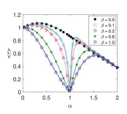
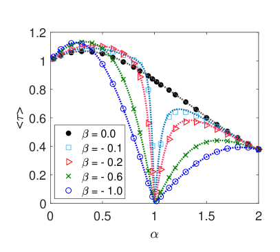
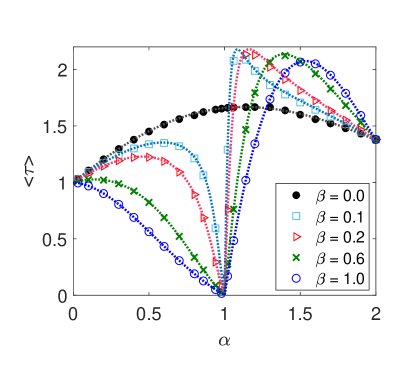
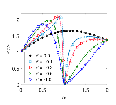
Figure 11: MFPT versus $\alpha$ with $d=0.5$ for two interval lengths. Top: $L=1$. Bottom: $L=3$. Dotted lines show the result (95) and symbols are the numerical solution of the space-fractional diffusion equation.

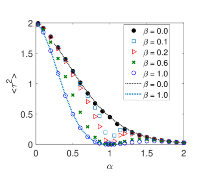
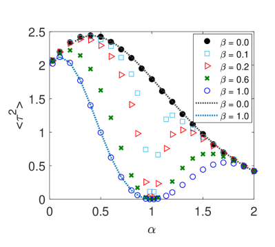
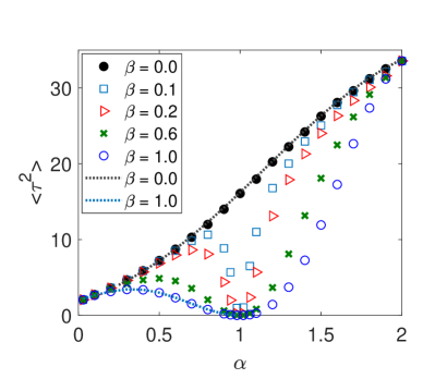
Figure 12: Second moment of the first-passage time PDF for interval length $L=0.5$ (top left), $L=1.0$ (top right) and $L=3$ (bottom) versus $\alpha$. The initial position is in the centre of the interval ($d=L$). Symbols show the numerical solution of the space-fractional diffusion equation and dotted lines show the analytic solution (82) for the symmetric case ($\beta=0$) and (87) with $m=2$ (one-sided $0<\alpha<1,\beta=1$).

We now change the scenario and set the initial position at a distance $d=0.5$ away from the right boundary. Figure 11 analyses the MFPT versus $\alpha$ and different skewness $\beta$ for two different interval lengths ($L=1$ and $L=3$). As can be seen, there is a perfect agreement between the results based on the numerical solution of the space-fractional diffusion equation and the analytic solution (95). In comparison with the symmetric initial position of the random process in figure 10, for positive values of the skewness parameter and when $\alpha\in(0,1)$, since the initial point is closer to the right boundary and the effective drift is in direction of the positive axis, the MFPT decreases. For $\alpha\in(1,2)$ and positive skewness, the effective drift is toward the left, and the MFPT increases rapidly. The opposite behaviour is observed when the skewness is negative (figure 11, right panels): for $\alpha\in(0,1)$ and $\alpha\in(1,2)$ with $\beta<0$, the effective drift is to the left and right directions, respectively.

In figure 12, analogous to figure 10, we show the results for the second moment of the first-passage time PDF versus the stability index $\alpha$ for different sets of the skewness parameter $\beta$ when the initial position is in the centre of the interval ($d=L$).

Finally, in figure 13 we show the coefficient of variation

$$f=\frac{\langle\tau^{2}\rangle-{\langle\tau\rangle}^{2}}{{\langle\tau\rangle}^{2}}.$$ (101)

When $f>1$ the underlying distribution is broad and we need to study higher order moments to get the complete information of the first-passage time PDF. When $f<1$, the distribution is narrow and higher order moments are not needed. For the one-sided $\alpha$-stable process ($0<\alpha<1$ and $\beta=1$) recalling equation (87), the coefficient of variation reads

$$f=\frac{\frac{\Gamma(1+2)}{\Gamma(1+2\alpha)}\frac{d^{2\alpha}}{\xi^{2}}-\left(\frac{\Gamma(1+1)}{\Gamma(1+\alpha)}\frac{d^{\alpha}}{\xi}\right)^{2}}{\left(\frac{\Gamma(1+1)}{\Gamma(1+\alpha)}\frac{d^{\alpha}}{\xi}\right)^{2}}=\frac{2\Gamma{(1+\alpha)}^{2}}{\Gamma{(1+2\alpha)}}-1,$$ (102)

which is always less than one, compare also figure 13. Thus, the MFPT is a fairly good measure for the first-passage process.

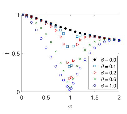
Figure 13: Coefficient of variation $f$ versus $\alpha$ for the first-passage time PDF with initial distance $L=d$.

7 Discussion and unsolved problems

LFs are relevant proxy processes to study the efficiency and spatial exploration behaviour of random search processes, from animals ("movement ecology") and humans to robots and computer algorithms. Apart from the MFPT such processes can be studied in terms of the mean inverse first-passage time $\langle 1/\tau\rangle$ as well as fractional order moments. Here we quantified the first-passage dynamics of symmetric and asymmetric LFs in both semi-infinite and finite domains and obtained the moments of the associated first-passage time PDF. These moments were analyses as functions of the process parameters, the stable index $\alpha$ and skewness $\beta$, as well as the system parameters, the initial distance $d$ and the interval length $L$ (if not infinite). As seen in the results the behaviour for different parameters can be quite rich and requires careful interpretation. Table 1 summarises the main features.

$\alpha$	$\beta$	Semi-infinite domain	Bounded domain
2	Irrelevant	(48),     $-\infty<q<1/2$ [43]	$\langle\tau\rangle\to$ (81) [65, 80, 43]
			$\langle\tau^{2}\rangle\to$ (83) [65, 43]
(0, 2)	0	Unknown,    $-1<q<1/2$	$\langle\tau\rangle\to$ (81) [65, 80, 83]
			$\langle\tau^{2}\rangle\to$ (82) [65]
(0,1)	1	(56), (87),   $-1<q<\infty$, ($q=m=1$ [48, 68])
(1, 2)	-1	(60), $-\infty<q<1/\alpha$	$\langle\tau\rangle\to$ (90)
	1	(67), $-1<q<1-1/\alpha$	$\langle\tau\rangle\to$ (91)
(0, 1)	(-1, 1)	Unknown, $-1<q<\rho$ [75]	$\langle\tau\rangle\to$ (95)
(1, 2)

Table 1: First-passage time PDF moments for different $\alpha$ and skewness $\beta$.

We here studied the one-dimensional case, for which the effect of LF versus Brownian search is expected to be most significant. One-dimensional is relevant for the vertical search of seaborne predators [12, 13] as well as random search along, for instance, natural boundaries such as field-forest boundaries or the shrubbery growing along streams. Other direct applications include search in computer algorithms [129, 130] or the effective one-dimensional search on linear polymer chains where LFs are effected by jumps to different chain segments at points where the polymer loops back onto itself [14, 131]. In a next step it will be of interest to extend these results to two dimensions, which is the relevant situation for a large number of search and movement processes. Another important direction of future research is to study the influence of interdependence on the first-passage properties for processes with infinite variance. Indeed, when the specific stochastic process is considered in a bounded domain the analysis of correlations in this process is important [132, 133]. Fractional LFs with long-range dependence have been detected in beat-to-beat heart rate fluctuations [134], in solar flare time series [135], and they have been shown to be a model qualitatively mimicking self-organized criticality signatures in data [136]. Apparently, correlations or spectral power analysis, strictly speaking, cannot be used for LFs, and alternative measures of dependence are necessary, see, e.g., the review [137].

In many situations for diffusive processes cognisance of the MFPT is insufficient to fully characterise the first-passage statistic. This statement was quantified in terms of the uniformity index statistic in [138, 139]. Instead, it is important to know the entire PDF of first-passage times, even in finite domains [140, 141, 142, 143]. Such notions are indeed relevant for biological processes, for instance, in scenarios underlying gene regulation, for which the detailed study reveals a clear dependence on the initial distance, which thus goes beyond the MFPT [144, 145, 146]. While we here saw that the coefficient of variation of the first-passage statistic is below unity, it will have to be seen, for instance, how this changes to situations of first-arrival to a partially reactive site. Another feature to be included are many-particle effects, for instance, flocking behaviour provoking different hunting strategies [147, 148, 149].

Appendix A Generator and backward Kolmogorov equation for an LF killed upon leaving the domain

Let $\tau=\min\{t:|x(t)|\geqslant L\}$ be the first-passage time of an LF $x(t)$. Let us define the corresponding killed process on $[-L,L]$ as

$$\bar{x}(t)=\left\{\begin{array}[]{lcl}x(t)&&{\rm if\;}t<\tau\\ \partial&&{\rm if\;}t\geq\tau\\ \end{array}\right..$$ (103)

Here, $\partial$ is the so-called "cemetery state". It is a domain outside of the interval $[-L,L]$. Note that the process $\bar{x}(t)$ describes the dynamics of the LF confined to the interval $[-L,L]$. When the LF leaves the domain, $\bar{x}(t)$ moves to the cemetery state and stays there forever.

The key property here is that $\bar{x}(t)$ is also a Markov process [150]. Therefore one can define its generator $D^{\alpha}_{x}$ in a usual way. This generator is equal to the generator of LFs confined to the interval $[-L,L]$ [150]. It has the form

$$D^{\alpha}_{x}f(x)=R_{\alpha,\beta}\,{}_{-L}D_{x}^{\alpha}f(x)+L_{\alpha,\beta}\,{}_{x}D_{L}^{\alpha}f(x),$$ (104)

for appropriately smooth function $f(x)$. Here ${}_{-L}D_{x}^{\alpha}$ and ${}_{x}D_{L}^{\alpha}$ are the fractional derivatives defined in (5) and (6), respectively. Moreover, $L_{\alpha,\beta}$ and $R_{\alpha,\beta}$ are the constants defined in equation (7). Here we employ an important property, namely, that under absorbing boundary conditions the adjoint operator of the left derivative (5) is equal to the right derivative (6) and vice versa [151].

Consequently, it follows from the general theory of Markov processes [152] that the PDF $P_{\alpha,\beta}(x,t|x_{0})$ of the killed process starting at $x_{0}$ satisfies the backward Kolmogorov equation

$$\frac{\partial P_{\alpha,\beta}(x,t|x_{0})}{\partial t}=K_{\alpha}\,D^{\alpha}_{x_{0}}P_{\alpha,\beta}(x,t|x_{0}),$$ (105)

where $D^{\alpha}_{x_{0}}$ is given by (104) with $x$ replaced by $x_{0}$. Finally, knowing the generator of $\bar{x}(t)$ and the corresponding backward Kolmogorov equation one can apply the usual method of finding the mean first-passage time of the LF described in detail in section 4.

Appendix B Derivation of MFPT for general $\alpha$-stable process in a finite interval

Here we compute the MFPT of LFs with stability index $\alpha\in(0,2]$ and skewness $\beta\in[-1,1]$ (excluding $\alpha=1$ with $\beta\neq 0$). To determine the parameters $\mu$ and $\nu$, by substitution of equation (73) into (72) we get

$$\frac{K_{\alpha}C_{\alpha,\beta}R_{\alpha,\beta}}{\Gamma(n-\alpha)}\int\limits_{-L}^{x_{0}}\frac{\left((L-\zeta)^{\mu}(L+\zeta)^{\nu}\right)^{(n)}}{(x_{0}-\zeta)^{\alpha-n+1}}\mathrm{d}\zeta$$

$$+\frac{(-1)^{n}K_{\alpha}C_{\alpha,\beta}L_{\alpha,\beta}}{\Gamma(n-\alpha)}\int\limits_{x_{0}}^{L}\frac{\left((L-\zeta)^{\mu}(L+\zeta)^{\nu}\right)^{(n)}}{(\zeta-x_{0})^{\alpha-n+1}}\mathrm{d}\zeta=-1.$$ (106)

Let us first consider the case $n=1$ ($0<\alpha<1$). By taking the first derivative

$$\frac{K_{\alpha}C_{\alpha,\beta}R_{\alpha,\beta}}{\Gamma(1-\alpha)}\int\limits_{-L}^{x_{0}}\frac{\nu(L-\zeta)^{\mu}(L+\zeta)^{\nu-1}-\mu(L-\zeta)^{\mu-1}(L+\zeta)^{\nu}}{(x_{0}-\zeta)^{\alpha}}\,\mathrm{d}\zeta$$

$$-\frac{K_{\alpha}C_{\alpha,\beta}L_{\alpha,\beta}}{\Gamma(1-\alpha)}\int\limits_{x_{0}}^{L}\frac{\nu(L-\zeta)^{\mu}(L+\zeta)^{\nu-1}-\mu(L-\zeta)^{\mu-1}(L+\zeta)^{\nu}}{(\zeta-x_{0})^{\alpha}}\,\mathrm{d}\zeta=-1,$$ (107)

then, by change of variables $y=(x_{0}-\zeta)/(x_{0}+L)$ and $y=(\zeta-x_{0})/(L-x_{0})$ in the first and second integral on the left hand side, respectively, we have

$$(L+x_{0})^{\nu-\alpha}(L-x_{0})^{\mu}$$

$$\times\int\limits_{0}^{1}\frac{\nu(1+\frac{L+x_{0}}{L-x_{0}}y)^{\mu}(1-y)^{\nu-1}-\mu\frac{L+x_{0}}{L-x_{0}}(1+\frac{L+x_{0}}{L-x_{0}}y)^{\mu-1}(1-y)^{\nu}}{y^{\alpha}}\mathrm{d}y,$$ (108)

and

$$(L+x_{0})^{\nu}(L-x_{0})^{\mu-\alpha}$$

$$\times\int\limits_{0}^{1}\frac{\nu\frac{L-x_{0}}{L+x_{0}}(1-y)^{\mu}(1+\frac{L-x_{0}}{L+x_{0}}y)^{\nu-1}-\mu(1-y)^{\mu-1}(1+\frac{L-x_{0}}{L+x_{0}}y)^{\nu}}{y^{\alpha}}\mathrm{d}y.$$ (109)

Then, defining $z=(L+x_{0})/(L-x_{0})$ and using the integral representation of the Gauss hypergeometric function [153] (see equation (9.1.6)),

$$F(a;b;c;x)=\frac{\Gamma(c)}{\Gamma(b)\Gamma(c-b)}\int\limits_{0}^{1}\frac{t^{b-1}(1-t)^{c-b-1}}{(1-xt)^{a}}\mathrm{d}t,$$ (110)

where $\mathrm{Re}(c)>\mathrm{Re}(b)>0$ and $|\arg(1-z)|<\pi$, we obtain

$$\frac{K_{\alpha}C_{\alpha,\beta}R_{\alpha,\beta}}{\Gamma(1-\alpha)}(L+x_{0})^{\nu-\alpha}(L-x_{0})^{\mu}\Big{[}\frac{\Gamma(1-\alpha)\Gamma(1+\nu)}{\Gamma(1+\nu-\alpha)}F(-\mu;1-\alpha;1+\nu-\alpha;-z)$$

$$-\mu z\frac{\Gamma(1-\alpha)\Gamma(1+\nu)}{\Gamma(2+\nu-\alpha)}F(1-\mu;1-\alpha;2+\nu-\alpha;-z)\Big{]}$$

$$-\frac{K_{\alpha}C_{\alpha,\beta}L_{\alpha,\beta}}{\Gamma(1-\alpha)}(L+x_{0})^{\nu}(L-x_{0})^{\mu-\alpha}\Big{[}\frac{\nu}{z}\frac{\Gamma(1-\alpha)\Gamma(1+\mu)}{\Gamma(2+\mu-\alpha)}F(1-\nu;1-\alpha;2+\mu-\alpha;-z^{-1})$$

$$-\frac{\Gamma(1-\alpha)\Gamma(1+\mu)}{\Gamma(1+\mu-\alpha)}F(-\nu;1-\alpha;1+\mu-\alpha;-z^{-1})\Big{]}=-1.$$ (111)

Moreover, by applying the relation [153] (see equation (9.5.9))

$$F(a;b;c;x)=(-x)^{-a}\frac{\Gamma(c)\Gamma(b-a)}{\Gamma(c-a)\Gamma(b)}F(a;1+a-c;1+a-b;x^{-1})$$

$$+(-x)^{-b}\frac{\Gamma(c)\Gamma(a-b)}{\Gamma(c-b)\Gamma(a)}F(b;1+b-c;1+b-a;x^{-1}),$$ (112)

where $|\arg(-x)|<\pi$, $|\arg(1-x)|<\pi$, and $a-b\neq 0,\pm 1,\pm 2,\dots$, one can write

$$\frac{\Gamma(1-\alpha)\Gamma(1+\nu)}{\Gamma(1+\nu-\alpha)}F(-\mu;1-\alpha;1+\nu-\alpha;-z)=z^{\mu}\frac{\Gamma(1+\mu-\alpha)\Gamma(1+\nu)}{\Gamma(1+\mu+\nu-\alpha)}$$

$$\times F(-\mu;\alpha-\mu-\nu;\alpha-\mu;-z^{-1})+z^{\alpha-1}\frac{\nu\Gamma(1-\alpha)\Gamma(\alpha-\mu-1)}{\Gamma(-\mu)}$$

$$\times F(1-\alpha;1-\nu;2+\mu-\alpha;-z^{-1}),$$ (113)

and

$$\mu z\frac{\Gamma(1-\alpha)\Gamma(1+\nu)}{\Gamma(2+\nu-\alpha)}F(1-\mu;1-\alpha;2+\nu-\alpha;-z)=\mu z^{\mu}\frac{\Gamma(1+\nu)\Gamma(\mu-\alpha)}{\Gamma(1+\mu+\nu-\alpha)}$$

$$\times F(1-\mu;\alpha-\mu-\nu;1+\alpha-\mu;-z^{-1})+\mu z^{\alpha}\frac{\Gamma(1-\alpha)\Gamma(\alpha-\mu)}{\Gamma(1-\mu)}$$

$$\times F(1-\alpha;-\nu;1+\mu-\alpha;-z^{-1}).$$ (114)

By substitution into equation (111)

$$\frac{K_{\alpha}C_{\alpha,\beta}R_{\alpha,\beta}}{\Gamma(1-\alpha)}(L+x_{0})^{\nu-\alpha}(L-x_{0})^{\mu}\Big{[}\nu z^{\mu}B(\nu,1+\mu-\alpha)F(-\mu;\alpha-\mu-\nu;\alpha-\mu;-z^{-1})$$

$$+\nu z^{\alpha-1}B(1-\alpha,\alpha-\mu-1)F(1-\alpha;1-\nu;2+\mu-\alpha;-z^{-1})$$

$$-\mu z^{\mu}B(1+\nu,\mu-\alpha)F(1-\mu;\alpha-\mu-\nu;1+\alpha-\mu;-z^{-1})-\mu z^{\alpha}B(1-\alpha,\alpha-\mu)$$

$$\times F(1-\alpha;-\nu;1+\mu-\alpha;-z^{-1})\Big{]}$$

$$-\frac{K_{\alpha}C_{\alpha,\beta}L_{\alpha,\beta}}{\Gamma(1-\alpha)}(L+x_{0})^{\nu}(L-x_{0})^{\mu-\alpha}\Big{[}\frac{\nu}{z}B(1-\alpha,1+\mu)F(1-\nu;1-\alpha;2+\mu-\alpha;-z^{-1})$$

$$-\mu B(1-\alpha,\mu)F(-\nu;1-\alpha;1+\mu-\alpha;-z^{-1})\Big{]}=-1.$$ (115)

Here, $B(a,b)=\Gamma(a)\Gamma(b)/\Gamma(a+b)$ is the Beta function and with the help of the symmetry property of the Gauss hypergeometric function, $F(a;b;c;x)=F(b;a;c;x)$ [153] (see equation (9.2.1)), we have

$$F(1-\alpha;1-\nu;2+\mu-\alpha;-z^{-1})=F(1-\nu;1-\alpha;2+\mu-\alpha;-z^{-1})$$

$$F(1-\alpha;-\nu;1+\mu-\alpha;-z^{-1})=F(-\nu;1-\alpha;1+\mu-\alpha;-z^{-1}).$$ (116)

By substitution into equation (115), we get

$$\frac{K_{\alpha}C_{\alpha,\beta}R_{\alpha,\beta}}{\Gamma(1-\alpha)}(L+x_{0})^{\mu+\nu-\alpha}\Big{[}\nu B(\nu,1+\mu-\alpha)F(-\mu;\alpha-\mu-\nu;\alpha-\mu;-z^{-1})$$

$$-\mu B(1+\nu,\mu-\alpha)F(1-\mu;\alpha-\mu-\nu;1+\alpha-\mu;-z^{-1})\Big{]}$$

$$+\frac{K_{\alpha}C_{\alpha,\beta}}{\Gamma(1-\alpha)}(L+x_{0})^{\nu-1}(L-x_{0})^{1+\mu-\alpha}\Big{[}\nu R_{\alpha,\beta}B(1-\alpha,\alpha-\mu-1)-\nu L_{\alpha,\beta}B(1-\alpha,1+\mu)\Big{]}$$

$$\times F(1-\nu;1-\alpha;2+\mu-\alpha;-z^{-1})-\frac{K_{\alpha}C_{\alpha,\beta}}{\Gamma(1-\alpha)}(L+x_{0})^{\nu}(L-x_{0})^{\mu-\alpha}$$

$$\times\Big{[}\mu R_{\alpha,\beta}B(1-\alpha,\alpha-\mu)-\mu L_{\alpha,\beta}B(1-\alpha,\mu)\Big{]}F(1-\alpha;-\nu;1+\mu-\alpha;-z^{-1})=-1.$$ (117)

Then, by rearranging we obtain

$$\frac{K_{\alpha}C_{\alpha,\beta}L_{\alpha,\beta}}{\Gamma(1-\alpha)}(L+x_{0})^{\mu+\nu-\alpha}\Big{[}\nu B(\nu,1+\mu-\alpha)F(-\mu;\alpha-\mu-\nu;\alpha-\mu;-z^{-1})$$

$$-\mu B(1+\nu,\mu-\alpha)F(1-\mu;\alpha-\mu-\nu;1+\alpha-\mu;-z^{-1})\Big{]}$$

$$+\frac{K_{\alpha}C_{\alpha,\beta}}{\Gamma(1-\alpha)}(L+x_{0})^{\nu}(L-x_{0})^{\mu-\alpha}\Big{[}\Big{(}\nu\Big{(}R_{\alpha,\beta}B(1-\alpha,\alpha-\mu-1)-L_{\alpha,\beta}B(1-\alpha,1+\mu)\Big{)}$$

$$\times z^{-1}F(1-\alpha;1-\nu;2+\mu-\alpha;-z^{-1})-\mu\Big{(}R_{\alpha,\beta}B(1-\alpha,\alpha-\mu)-L_{\alpha,\beta}B(1-\alpha,\mu)\Big{)}$$

$$\times F(1-\alpha;-\nu;1+\mu-\alpha;-z^{-1})\Big{]}=-1.$$ (118)

The left hand side must be independent of $z$ since $\mu$ and $\nu$ do not depend on $z$. This requirement leads to the relations below. For the first term on the left hand side, with the help of $F(a,b=0,c,x)=1$ [153] (see section (9.8)), we have

$$F(-\mu;\alpha-\mu-\nu;\alpha-\mu;-z^{-1})=1$$

$$F(1-\mu;\alpha-\mu-\nu;1+\alpha-\mu;-z^{-1})=1,$$ (119)

where

$$b=\alpha-\mu-\nu=0\to\alpha=\mu+\nu.$$ (120)

For the second term, we find

$$R_{\alpha,\beta}B(1-\alpha,\alpha-\mu-1)-L_{\alpha,\beta}B(1-\alpha,1+\mu)=0$$

$$R_{\alpha,\beta}B(1-\alpha,\alpha-\mu)-L_{\alpha,\beta}B(1-\alpha,\mu)=0.$$ (121)

By definition of the Beta function,

$$R_{\alpha,\beta}\frac{\Gamma(1-\alpha)\Gamma(\alpha-\mu-1)}{\Gamma(-\mu)}=L_{\alpha,\beta}\frac{\Gamma(1-\alpha)\Gamma(1+\mu)}{\Gamma(2+\mu-\alpha)}$$

$$R_{\alpha,\beta}\frac{\Gamma(1-\alpha)\Gamma(\alpha-\mu)}{\Gamma(1-\mu)}=L_{\alpha,\beta}\frac{\Gamma(1-\alpha)\Gamma(\mu)}{\Gamma(1+\mu-\alpha)}.$$ (122)

Using Euler’s reflection formula $\Gamma(1-z)\Gamma(z)\sin{(\pi z)}=\pi$, we obtain

$$\frac{R_{\alpha,\beta}}{\sin{(\pi(\alpha-\mu-1))}}=\frac{L_{\alpha,\beta}}{-\sin{(\pi\mu)}}$$

$$\frac{R_{\alpha,\beta}}{\sin{(\pi(\alpha-\mu))}}=\frac{L_{\alpha,\beta}}{\sin{(\pi\mu)}},$$ (123)

which are identical. With the help of the weight coefficients (see equation (7))

$$L_{\alpha,\beta} = -\frac{\sin{(\pi\alpha\rho)}}{\sin{(\pi\alpha)}\cos{(\pi\alpha(\rho-1/2))}}$$

$$R_{\alpha,\beta} = -\frac{\sin{(\pi\alpha(1-\rho))}}{\sin{(\pi\alpha)}\cos{(\pi\alpha(\rho-1/2))}},$$ (124)

where $\rho$ is defined in equation (50). Substitution into equation (123), we find

$$\frac{\sin{(\pi\alpha(1-\rho))}}{\sin{(\pi(\alpha-\mu))}}=\frac{\sin{(\pi\alpha\rho)}}{\sin{(\pi\mu)}}.$$ (125)

Therefore, the parameters $\mu$ and $\nu$ have the following form (see equation (120))

$$\mu=\alpha\rho,\,\,\,\nu=\alpha-\alpha\rho.$$ (126)

To determine the normalisation factor, by substituting equation (74) into equation (118) we obtain

$$\frac{K_{\alpha}C_{\alpha,\beta}R_{\alpha,\beta}}{\Gamma(1-\alpha)}\Big{[}\nu B(\nu,1+\mu-\alpha)-\mu B(1+\nu,\mu-\alpha)\Big{]}=-1.$$ (127)

Using the Beta function,

$$\frac{K_{\alpha}C_{\alpha,\beta}R_{\alpha,\beta}}{\Gamma(1-\alpha)}\Big{[}-\alpha\Gamma(1+\nu)\Gamma(\mu-\alpha)\Big{]}=-1,$$ (128)

we get

$$C_{\alpha,\beta}=\frac{\Gamma(1-\alpha)}{\alpha K_{\alpha}R_{\alpha,\beta}\Gamma(1+\alpha-\alpha\rho)\Gamma(\alpha\rho-\alpha)}=\frac{1}{\Gamma(1+\alpha)K_{\alpha}}\frac{\sin{(\pi\alpha(\rho-1))}}{R_{\alpha,\beta}\sin{(\pi\alpha)}},$$ (129)

where the last equality follows from Euler’s reflection formula. Finally by substitution of $R_{\alpha,\beta}$ (equation (124)), we get the desire result (75).

Appendix C Fractional integration of a fractional derivative

Here we show the composition rule for the right Riemann-Liouville fractional integral and the right fractional derivative in the Caputo form of the operator. The right Riemann-Liouville fractional integral is given by ($p\in\mathrm{Re}>0$) [96]

$${}_{x}D_{L}^{-p}f(x)=\frac{1}{\Gamma(p)}\int\limits_{x}^{L}\frac{f(\zeta)}{(\zeta-x)^{1-p}}\mathrm{d}\zeta,$$ (130)

and with the right Caputo form of the fractional derivative as ($n-1<q<n$)

$$_{x}D_{L}^{q}f(x)=\frac{(-1)^{n}}{\Gamma(n-q)}\int\limits_{x}^{L}\frac{f^{(n)}(\zeta)}{(\zeta-x)^{q-n+1}}\mathrm{d}\zeta,$$ (131)

we write

$${}_{x}D_{L}^{-p}\left({}_{x}D_{L}^{q}f(x)\right)=\frac{1}{\Gamma(p)}\int\limits_{x}^{L}\frac{{}_{\zeta}D_{L}^{q}f(\zeta)}{(\zeta-x)^{1-p}}\mathrm{d}\zeta.$$ (132)

Then, with the help of equation (131) we find

$${}_{x}D_{L}^{-p}\left({}_{x}D_{L}^{q}f(x)\right)=\frac{(-1)^{n}}{\Gamma(p)\Gamma(n-q)}\int_{x}^{L}\frac{1}{(\zeta-x)^{1-p}}\int\limits_{\zeta}^{L}\frac{f^{(n)}(y)}{(y-\zeta)^{q-n+1}}\mathrm{d}y\mathrm{d}\zeta.$$ (133)

Now, we change the integration order,

$$\int\limits_{x}^{L}\int\limits_{\zeta}^{L}f(x,\zeta,y)\mathrm{d}y\mathrm{d}\zeta=\int\limits_{x}^{L}\int\limits_{x}^{y}f(x,\zeta,y)\mathrm{d}\zeta\mathrm{d}y,$$ (134)

and get

$${}_{x}D_{L}^{-p}\left({}_{x}D_{L}^{q}f(x)\right)=\frac{(-1)^{n}}{\Gamma(p)\Gamma(n-q)}\int\limits_{x}^{L}f^{(n)}(y)\int\limits_{x}^{y}\frac{1}{(\zeta-x)^{1-p}(y-\zeta)^{q-n+1}}\mathrm{d}\zeta\mathrm{d}y.$$ (135)

After change of variable, $\zeta=x+z(y-x)$ in the inner integral, we arrive at

$${}_{x}D_{L}^{-p}\left({}_{x}D_{L}^{q}f(x)\right)=\frac{(-1)^{n}}{\Gamma(p)\Gamma(n-q)}\int\limits_{x}^{L}\frac{f^{(n)}(y)}{(y-x)^{1-n}}\int\limits_{0}^{1}\frac{1}{z^{1-p}(1-z)^{q-n+1}}\mathrm{d}z\mathrm{d}y.$$ (136)

Then, with the help of

$$\int\limits_{0}^{1}\frac{1}{z^{1-p}(1-z)^{q-n+1}}\mathrm{d}z=\frac{\Gamma(p)\Gamma(n-q)}{\Gamma(n)},$$ (137)

we find

$${}_{x}D_{L}^{-p}\left({}_{x}D_{L}^{q}f(x)\right)=\frac{(-1)^{n}}{\Gamma(n)}\int\limits_{x}^{L}\frac{f^{(n)}(y)}{(y-x)^{1-n}}\mathrm{d}y.$$ (138)

For our case in section 6.2.1 with $p=q=m\alpha$ and $f(x_{0})=\langle\tau^{m}\rangle(x_{0})$, when $n=1$ ($0<\alpha<1$, $m=1$) this becomes

$${}_{x_{0}}D_{L}^{-m\alpha}\left({}_{x_{0}}D_{L}^{m\alpha}\langle\tau^{m}\rangle(x_{0})\right)=\langle\tau^{m}\rangle(x_{0})-\langle\tau^{m}\rangle(L),$$ (139)

and when $n=2$ ($0<\alpha<1$, $m=2$) after integration by part we get

$${}_{x_{0}}D_{L}^{-m\alpha}\left({}_{x_{0}}D_{L}^{m\alpha}\langle\tau^{m}\rangle(x_{0})\right)=(L-x_{0})\frac{\partial\langle\tau^{m}\rangle(y)}{\partial y}\Big{|}_{y=L}+\langle\tau^{m}\rangle(x_{0})-\langle\tau^{m}\rangle(L).$$ (140)

With a similar procedure for $n\geq 3$ it can be deduce that in order to get result (85), all derivatives of the order $n-1<m\alpha$ of $\langle\tau^{m}\rangle(y)$ at $y=L$ should be zero. The fact that $\langle\tau^{m}\rangle(y)$ vanishes at $y=L$ is intuitively clear, when the initial point of the random walker is located right at the absorbing boundary $x_{0}=L$, it will be removed immediately. We also note that by differentiating the result (87) it is easy to check that the assumption that all derivatives of $\langle\tau^{m}\rangle(y)$ vanish at $y=L$ is reasonable.

References

References

- [1] Mandelbrot BB 1997 The Fractal Geometry of Nature (New York: Freeman)
- [2] Hughes BD 1995 Random Walks and Random Environments (Vol 1: RandomWalks) (Oxford: Oxford University Press)
- [3] Bouchaud JP and Georges A 1990 Anomalous diffusion in disordered media: Statistical mechanisms, models and physical applications Phys. Rep. 195 127
- [4] Metzler R and Klafter J 2000 The random walk’s guide to anomalous diffusion: a fractional dynamics approach Phys. Rep. 339 1
- [5] Metzler R and Klafter J 2004 The restaurant at the end of the random walk: recent developments in the description of anomalous transport by fractional dynamics J. Phys. A 37 R161
- [6] Lesmoir-Gordon N 2018 Clouds Are Not Spheres: A Portrait of Benoît Mandelbrot, The Founding Father of Fractal Geometry (Singapore: World Scientific)
- [7] Vahabi M, Schulz JHP, Shokri B, and Metzler R 2013 Area coverage of radial Lévy flights with periodic boundary conditions Phys. Rev. E 87 042136
- [8] Shlesinger MF and Klafter J 1986 in On Growth and Form, edited by Stanley HE and Ostrowsky N (Dordrecht, Netherlands: Martinus Nijhoff)
- [9] Viswanathan GM et al. 1996 Lévy flight search patterns of wandering albatrosses Nature 381 413
- [10] Viswanathan GM et al. 1999 Optimizing the success of random searches Nature 401 911
- [11] Edwards AM et al. 2007 Revisiting Lévy flight search patterns of wandering albatrosses, bumblebees and deer Nature 449 1044
- [12] Humphries NE, Weimerskirch H, Queiroz N, Southall EJ, and Sims DW 2012 Foraging success of biological Lévy flights recorded in situ Proc. Natl. Acad. Sci. USA 109 7169
- [13] Sims DW, Witt MJ, Richardson AJ, Southall EJ, and Metcalfe JD 2006 Encounter success of free-ranging marine predator movements across a dynamic prey landscape Proc. Biol. Sci. 273 1195
- [14] Lomholt MA, Ambjörnsson T, and Metzler R 2005 Optimal target search on a fast folding polymer chain with volume exchange Phys. Rev. Lett. 95 260603
- [15] Lomholt MA, Koren T, Metzler R, and Klafter J 2008 Lévy strategies in intermittent search processes are advantageous Proc. Natl. Acad. Sci. USA 105 11055
- [16] Palyulin VV, Chechkin AV, Klages R, and Metzler R 2016 Search reliability and search efficiency of combined Lévy-Brownian motion: long relocations mingled with thorough local exploration J. Phys. A 49 394002
- [17] Palyulin VV, Mantsevich VN, Klages R, Metzler R, and Chechkin AV 2017 Comparison of pure and combined search strategies for single and multiple targets Eur. Phys. J. B 90 170
- [18] Viswanathan GE, da Luz MGE, Raposo EP, and Stanley HE 2011 The Physics of Foraging: An Introduction to Random Searches and Biological Encounters (Cambridge UK: Cambridge University Press)
- [19] Palyulin VV, Chechkin AV, and Metzler R 2014 Lévy flights do not always optimize random blind search for sparse targets Proc. Natl. Acad. Sci. USA 111 2931
- [20] Palyulin VV, Checkin AV, and Metzler R 2014 Optimization of random search processes in the presence of an external bias J. Stat. Mech. 2014 P11031
- [21] Hufnagel L, Brockmann D, and Geisel T 2004 Forecast and control of epidemics in a globalized world Proc. Natl. Acad. Sci. USA 101 15124
- [22] Brockmann D, Hufnagel L, and Geisel T 2006 The scaling laws of human travel Nature 439 462
- [23] González MC, Hidalgo CA, and Barabási AL 2008 Understanding individual human mobility patterns Nature 453 779
- [24] Barthelemy P, Bertolotti J, and Wiersma DS 2008 A Lévy flight for light Nature 453 495
- [25] Katori H, Schlipf S, and Walther H 1997 Anomalous dynamics of a single ion in an optical lattice Phys. Rev. Lett. 79 2221
- [26] Mandelbrot BB 1963 The variation of certain speculative prices J. Business 36 394
- [27] Fama EF 1965 The behaviour of stock market prices J. Business 38 34
- [28] Mantegna RN and Stanley HE 1995 Scaling behaviour in the dynamics of an economic index Nature 376 46
- [29] Lévy PP 1954 Théorie de l’addition des variables aléatoires (Paris: Gauthier-Villars)
- [30] Gnedenko BV and Kolmogorov AN 1954 Limit Distributions for Sums of Random Variables (Cambridge, MA: Addison-Wesley)
- [31] Samorodnitsky G and Taqqu MS 1994 Stable Non-Gaussian Random Processes: Stochastic Models with Infinite Variance (New York: Chapman and Hall)
- [32] Gikhman II and Skorokhod AV 1975 Theory of Stochastic Processes II (Berlin: Springer)
- [33] Zolotarev VM 1986 One-Dimensional Stable Distributions (Providence, RI: American Mathematical Society)
- [34] Paradisi P, Cesari R, Mainardi F, Maurizi A, and Tampieri F 2001 A generalized Fick’s law to describe non-local transport effects Phys. Chem. Earth (B) 26 275
- [35] Paradisi P, Cesari R, Mainardi F, and Tampieri F 2001 The fractional Fick’s law for non-local transport processes Physica A 293 130
- [36] Khintchine AYa 1935 On the domain of attraction of the Gauss law Giornale dell’Istituto Italiano degli Attuari Vol 6 378
- [37] Mantegna RN and Stanley HE 1994 Stochastic process with ultraslow convergence to a Gaussian: the truncated Lévy flight Phys. Rev. Lett. 73 2946
- [38] Koponen I 1995 Analytic approach to the problem of convergence of truncated Lévy flights towards the Gaussian stochastic process Phys. Rev. E 52 1197
- [39] Sokolov IM, Chechkin AV, and Klafter J 2004 Fractional diffusion equation for a power-law-truncated Lévy process Physica A 336 245
- [40] Chechkin AV, Gonchar VYu, Klafter J, Metzler R, and Tanatarov LV 2004 Lévy flights in a steep potential well, J. Stat. Phys. 115 1505
- [41] Chechkin AV, Gonchar VYu, Klafter J, and Metzler R 2005 Natural cutoff in Lévy flights caused by dissipative non-linearity Phys. Rev. E 72 010101(R)
- [42] Feller W 1971 An Introduction to Probability Theory and its Applications vol 2 (New York: Wiley)
- [43] Redner S 2001 A Guide to First-Passage Processes (Cambridge: Cambridge University Press)
- [44] Gardiner C 2009 Stochastic Methods, A Handbook for the Natural and Social Sciences (Berlin: Springer)
- [45] Metzler R, Redner S, and Oshanin G 2014 First-Passage Phenomena and Their Applications (Singapore: World Scientific)
- [46] Chechkin AV, Metzler R, Klafter J, Gonchar VYu, and Tanatarov LV 2003 First passage time density for Lévy flight processes and the failure of the method of images J. Phys. A 36 L537
- [47] Koren T, Chechkin AV, and Klafter J 2007 On the first-passage time and leapover properties of Lévy motions Physica A 379 10
- [48] Koren T, Lomholt MA, Chechkin AV, Klafter J and Metzler R 2007 Leapover lengths and first-passage time statistics for Lévy flights Phys. Rev. Lett. 99 160602
- [49] Bingham NH 1973 Limit theorems in fluctuation theory Adv. Appl. Prob. 5 554
- [50] Bingham NH 1973 Maxima of sums of random variables and suprema of stable processes Z. Wahrscheinlichkeitsth. Verwandte Geb. 26 273
- [51] Prabhu NH 1981 Stochastic Storage Processes, Queues, Insurance Risk, Dams, and Data Communication (Berlin: Springer)
- [52] Bertoin J 1996 Lévy Processes (Cambridge: Cambridge University Press)
- [53] Frisch U and Frisch H 1995 Lévy Flights and Related Topics in Physics (Berlin: Springer)
- [54] Zumofen G and Klafter J 1995 Absorbing boundary in one-dimensional anomalous transport Phy. Rev. E 51 2805
- [55] Andersen ES 1953 On the fluctuations of sums of random variables I Math. Scand. 1 263
- [56] Andersen ES 1954 On the fluctuations of sums of random variables II Math. Scand. 2 195
- [57] Dybiec B, Gudowska-Nowak E, and Chechkin AV 2016 To hit or to pass it over–remarkable transient behaviour of first arrivals and passages for Lévy flights in finite domains J. Phys. A 49 504001
- [58] Majumdar SN 2010 Universal first-passage properties of discrete-time random walks and Lévy flights on a line: Statistics of the global maximum and records Physica A 389 4299
- [59] Majumdar SN, Mounaix P, and Schehr G 2017 Survival probability of random walks and Lévy flights on a semi-infinite line J. Phys. A 50 465002
- [60] Padash A, Chechkin AV, Dybiec B, Pavlyukevich I, Shokri B, and Metzler R 2019 First-passage properties of asymmetric Lévy flights J. Phys. A 52 454004
- [61] Kac M and Pollard H 1950 The distribution of the maximum of partial sums of independent random variables Canadian J. Math. 2 375
- [62] Spitzer F 1958 Some theorems concerning 2-dimensional Brownian motion Trans. Amer. Math. Soc. 87 187
- [63] Elliott J 1959 Absorbing barrier processes connected with the symmetric stable densities Illinois J. Math. 3 200
- [64] Blumenthal RM, Getoor RK, and Ray DB 1961 On the distribution of first hits for the symmetric stable processes Trans. Amer. Math. Soc. 99 540
- [65] Getoor RK 1961 First passage times for symmetric stable processes in space Trans. Amer. Math. Soc. 101 75
- [66] Dynkin EB 1961 Some limit theorems for sums of independent random variables with infinite mathematical expectations Select. Transl. Math. Statist. and Probability 1 Inst. Math. Statist. and Amer. Math. Soc. Providence R.I. 171
- [67] Ikeda N and Watanabe S 1962 On some relations between the harmonic measure and the Lévy measure for a certain class of Markov processes J. Math. Kyoto Univ. 2 79
- [68] Port SC 1970 The exit distribution of an interval for completely asymmetric stable processes Ann. Math. Statist. 41 39
- [69] Takács L 1966 Combinatorial Methods in the Theory of Stochastic Processes (New York: Wiley)
- [70] Bingham NH 1975 Fluctuation theory in continuous time Adv. Appl. Prob. 7 705
- [71] Bertoin J 1996 On the first exit time of a completely asymmetric stable process from a finite interval Bull. London Math. Soc. 28 514
- [72] Lambert A 2000 Completely asymmetric Lévy processes confined in a finite interval Ann. Inst. H. Poincaré. Prob. Stat. 36 251
- [73] Avram F, Kyprianou AE, and Pistorius MR 2004 Exit problems for spectrally negative Lévy processes and applications to (Canadized) Russian options Ann. Appl. Probab. 14 215
- [74] Tejedor V, Bénichou O, Metzler R, and Voituriez R 2011 Residual mean first-passage time for jump processes: theory and applications to Lévy flights and fractional Brownian motion J. Phys. A 44 255003
- [75] Doney RA and Maller RA 2004 Moments of passage times for Lévy processes Ann. Inst. Henri Poincaré. 40 279
- [76] Bogdan K, Byczkowski T, Kulczycki T, Ryznar M, Song R, and Vondracek Z 2009 Potential Analysis of Stable Processes and its Extensions, Lecture Notes in Mathematics 1980 (Berlin: Springer)
- [77] Profeta C and Simon T 2015 On the harmonic measure of stable processes. In Donati-Martin C, Lejay A, and Rouault A (editors), Séminaire de probabilités XLVIII, Lecture Notes in Mathematics 2168, pp 325 (Springer, Cham CH)
- [78] Kyprianou AE, Pardo JC, and Watson AR 2014 Hitting distributions of -stable processes via path-censoring and self-similarity Ann. Probab. 42 398
- [79] Buldyrev SV, Gitterman M, Havlin S, Kazakov AY, da Luz MGE, Raposo EP, Stanley HE, and Viswanathan GM 2001 Properties of Lévy flights on an interval with absorbing boundaries Physica A 302 148
- [80] Buldyrev SV, Havlin S, Kazakov AY, da Luz MGE, Raposo EP, Stanley HE, and Viswanathan GM 2001 Average time spent by Lévy flights and walks on an interval with absorbing boundaries Phys. Rev. E 64 041108
- [81] Dybiec B, Gudowska-Nowak E, and Hnggi P 2006 Lévy-Brownian motion on finite intervals: mean first-passage time analysis Phys. Rev. E 73 046104
- [82] Dybiec B, Gudowska-Nowak E, Barkai E, and Dubkov AA 2017 Lévy flights versus Lévy walks in bounded domains Phys. Rev. E 95 052102
- [83] Zoia A, Rosso A, and Kardar M 2007 Fractional Laplacian in bounded domains Phys. Rev. E 76 021116
- [84] Chen ZQ, Kim P, and Song R 2010 Heat kernel estimates for the Dirichlet fractional Laplacian J. Eur. Math. Soc. 12 1307
- [85] Katzav E and Adda-Bedia M 2008 The spectrum of the fractional Laplacian and first-passage-time statistics Europhys. Lett. 83 30006
- [86] Dubkov AA, La Cognata A, and Spagnolo B 2009 The problem of analytical calculation of barrier crossing characteristics for Lévy flights J. Stat. Mech. 2009 P01002
- [87] Xu Y, Feng J, Li J, and Zhang H 2013 Lévy noise induced switch in the gene transcriptional regulatory system Chaos 23 013110
- [88] Tingwei G, Jiaxiu D, Xiangyang L, and Ruifeng S 2014 Mean exit time and escape probability for dynamical systems driven by Lévy noise SIAM J. Sci. Comput. 36 A887
- [89] Xiao W, Jinqiao D, Xiaofan L, and Yuanchao L 2015 Numerical methods for the mean exit time and escape probability of two-dimensional stochastic dynamical systems with non-Gaussian noises Appl. Math. Comput. 258 282
- [90] Xiao W, Jinqiao D, Xiaofan L, and Ruifeng S 2018 Numerical algorithms for mean exit time and escape probability of stochastic systems with asymmetric Lévy motion Appl. Math. Comput. 337 618
- [91] Kim Y, Koprulu I, and Shroff NB 2015 First exit time of a Lévy flight from a bounded region in J. Appl. Probab. 52 649
- [92] Compte A 1996 Stochastic foundations of fractional dynamics Phys. Rev. E 53 4191
- [93] Metzler R, Barkai E, and Klafter J 1999 Anomalous diffusion and relaxation close to thermal equilibrium: A fractional Fokker-Planck equation approach Phys. Rev. Lett. 82 3563
- [94] Metzler R, Barkai E, and Klafter J 1999 Deriving fractional Fokker-Planck equations from a generalised master equation Europhys. Lett. 46 431
- [95] Kolokoltsov V 2015 On fully mixed and multidimensional extensions of the Caputo and Riemann-Liouville derivatives, related Markov processes and fractional differential equations Fract. Calc. Appl. Anal. 18 1039 1039
- [96] Podlubny I 1999 Fractional Differential Equations (New York: Academic Press)
- [97] del Castillo Negrete D 2006 Fractional diffusion models of nonlocal transport Phys. Plasmas 13 082308
- [98] Cartea Á and del Castillo Negrete D 2007 Fluid limit of the continuous-time random walk with general Lévy jump distribution functions Phys. Rev. E 76 041105
- [99] Samko SG, Kilbas AA, and Marichev OI 1993 Fractional Integrals and Derivatives, Theory and Applications (Amsterdam: Gordon and Breach)
- [100] Kwaśnicki M 2017 Ten equivalent definitions of the fractional Laplace operator Fract. Calc. Appl. Anal. 20 7
- [101] Hilfer R 2015 Experimental implications of Bochner-Lévy-Riesz diffusion Fract. Calc. Appl. Anal. 18 333
- [102] Song F, Xu C, and Karniadakis GE 2017 Computing fractional Laplacians on complex-geometry domains: algorithms and simulations SIAM J. Sci. Comput. 39 A1320
- [103] Cusimano N, del Teso F, Gerardo-Giorda L, and Pagnini G 2018 Discretizations of the spectral fractional Laplacian on general domains with Dirichlet, Neumann, and Robin boundary conditions SIAM J. Numer. Anal. 56 1243
- [104] Jia J and Wang H 2015 Fast finite difference methods for space-fractional diffusion equations with fractional derivative boundary conditions J. Comput. Phys. 293 359
- [105] Shimin G, Liquan M, Zhengqiang Z, and Yutao J 2018 Finite difference/spectral-Galerkin method for a two-dimensional distributed-order time-space fractional reaction-diffusion equation Appl. Math. Lett. 85 157
- [106] Deng WH 2008 Finite element method for the space and time fractional Fokker-Planck equation SIAM J. Numer. Anal. 47 204
- [107] Melean W and Mustapha K 2007 A second-order accurate numerical method for a fractional wave equation Numer. Math. 105 418
- [108] Fix GJ and Roop JP 2004 Least squares finite element solution of a fractional order two-point boundary value problem Comput. Math. Appl. 48 1017
- [109] Bhrawy AH, Zaky MA, and Van Gorder RA 2016 A space-time Legendre spectral tau method for the two-sided space-time Caputo fractional diffusion-wave equation Numer. Algor. 71 151
- [110] Li X and Xu C 2009 A space-time spectral method for the time fractional diffusion equation SIAM J. Numer. Anal. 47 2018
- [111] Oldham KB and Spanier J 1974 The Fractional Calculus: Theory and Applications of Differentiation and Integration to Arbitrary Order (New York: Academic)
- [112] Langlands TAM and Henry BI 2005 The accuracy and stability of an implicit solution method for the fractional diffusion equation J. Comput. Phys. 205 719
- [113] Li C and Zeng F 2012 Finite difference methods for fractional differential equations Int. J. Bifurcation Chaos 22 1230014
- [114] Lynch VE, Carreras BA, del-Castillo-Negrete D, Ferreira-Mejias KM, and Hicks HR 2003 Numerical methods for the solution of partial differential equations of fractional order J. Comput. Phys. 192 406
- [115] Sousa E 2010 How to approximate the fractional derivative of order Int. J. Bifurcation Chaos 22 1250075
- [116] Fogedby HC 1994 Lévy flights in random environments Phys. Rev. Lett. 73 2517
- [117] Jespersen S, Metzler R, and Fogedby HC 1999 Lévy flights in external force fields: Langevin and fractional Fokker-Planck equations and their solutions Phys. Rev. E 59 2736
- [118] Janicki A and Weron A 1994 Simulation and Chaotic Behavior of -stable Stochastic Processes (New York: Marcel Dekker)
- [119] Janicki A 1996 Numerical and Statistical Approximation of Stochastic Differential Equations with Non-Gaussian Measures (Wroclaw: Hugo Steinhaus Center)
- [120] Kloeden P and Platen E 2011 Numerical Solution of Stochastic Differential Equations Stochastic Modelling and Applied Probability (Berlin: Springer)
- [121] Maruyama G 1955 Continuous Markov processes and stochastic equations Rend. Circ. Mat. Palermo 4 48
- [122] Skorokhod AV 1964 Random Processes with Independent Increments (Moscow: Nauka) (in Russian)
- [123] Palyulin VV, Blackburn G, Lomholt MA, Watkins NW, Metzler R, Klages R, and Chechkin AV 2019 First passage and first hitting times of Lévy flights and Lévy walks New J. Phys. 21 103028
- [124] Mainardi F 2010 Fractional Calculus and Waves in Linear Viscoelasticity: An Introduction to Mathematical Models (London: Imperial College Press)
- [125] Mathai AM, Saxena RK, and Haubold HJ 2010 The H-Function: Theory and Applications (Berlin: Springer)
- [126] Simon T 2011 Hitting densities for spectrally positive stable processes Stochastics 83 203
- [127] Skorokhod AV 1954 Asymptotic formulas for stable distribution laws Dokl. Akad. Nauk SSSR 98 731
- [128] Mainardi F, Luchko Y, and Pagnini G 2001 The fundamental solution of the space-time fractional diffusion equation Fract. Calc. Appl. Anal. 4 153
- [129] Pavlyukevich I 2007 Lévy flights, non-local search and simulated annealing J. Comput. Phys. 226 1830
- [130] Pavlyukevich I 2008 Simulated annealing for Lévy-driven jump-diffusions Stoch. Proc. Applic. 118 1071
- [131] Sokolov IM, Mai J, and Blumen A 1997 Paradoxal diffusion in chemical space for nearest-neighbor walks over polymer chains Phys. Rev. Lett. 79 857
- [132] Vojta T, Skinner S, and Metzler R 2019 Probability density of the fractional Langevin equation with reflecting walls Phys. Rev. E 100 042142
- [133] Guggenberger T, Pagnini G, Vojta T, and Metzler R 2019 Fractional Brownian motion in a finite interval: correlations effect depletion or accretion zones of particles near boundaries, New J. Phys 21 022002
- [134] Peng CK, Mietus J, Hausdorff JM, Havlin S, Stanley HE, and Goldberger AL 1993 Long-range anticorrelations and non-Gaussian behavior of the heartbeat Phys. Rev. Lett. 70 1343
- [135] Burnecki K, Klafter J, Magdziarz M, and Weron A 2008 From solar flare time series to fractional dynamics Physica A 387 1077
- [136] Watkins NW, Credgington D, Sánchez R, Rosenberg SJ, and Chapman SC 2009 Kinetic equation of linear fractional stable motion and applications to modeling the scaling of intermittent bursts Phys. Rev. E 79 041124
- [137] Wyłomańska A, Chechkin A, Gajda J, and Sokolov IM 2015 Codifference as a practical tool to measure interdependence Physica A 421 412
- [138] Mejia-Monasterio C, Oshanin G, and Schehr G 2011 First passages for a search by a swarm of independent random searchers J. Stat. Mech. 2011 P06022
- [139] Mattos T, Mejía-Monasterio C, Metzler R, and Oshanin G 2012 First passages in bounded domains: When is the mean first-passage time meaningful? Phys. Rev. E 86 031143
- [140] Godec A and Metzler R 2016 First passage time distribution in heterogeneity controlled kinetics: going beyond the mean first-passage time Sci. Rep. 6 20349
- [141] Godec A and Metzler R 2016 Universal proximity effect in target search kinetics in the few encounter limit Phys. Rev. X 6 041037
- [142] Grebenkov D, Metzler R, and Oshanin G 2018 Towards a full quantitative description of single-molecule reaction kinetics in biological cells Phys. Chem. Chem. Phys. 20 16393
- [143] Grebenkov D, Metzler R, and Oshanin G 2018 Strong defocusing of molecular reaction times: geometry and reaction control Comm. Chem. 1 96
- [144] Kolesov G, Wunderlich Z, Laikova ON, Gelfand MS, and Mirny LA 2007 How gene order is influenced by the biophysics of transcription regulation Proc. Natl. Acad. Sci. USA 104 13948
- [145] Pulkkinen O and Metzler R 2013 Distance matters: the impact of gene proximity in bacterial gene regulation Phys. Rev. Lett. 110 198101
- [146] Kar P, Cherstvy AG, and Metzler R 2018 Acceleration of bursty multi-protein target-search kinetics on DNA by colocalisation Phys. Chem. Chem. Phys. 20 7931
- [147] Oshanin G, Vasilyev O, Krapivsky PL, and Klafter J 2009 Survival of an evasive prey Proc. Natl. Acad. Sci. USA 106 13696
- [148] Janosov M, Viragh C, Vasarhelyi G, and Vicsek T 2017 Group chasing tactics: how to catch a faster prey New J. Phys. 19 053003
- [149] Schwarzl M, Godec A, Oshanin G, and Metzler R 2016 A single predator charging a herd of prey: effects of self volume and predator-prey decision-making J. Phys. A. 49 225601
- [150] Baeumer B, Luks T, and Meerschaert M 2018 Space-time fractional Dirichlet problems Math. Nachrichten 291 2516
- [151] Podlubny I and Chen YQ 2007 Adjoint fractional differential expressions and operators Proceedings of the ASME 2007 International Design Engineering Technical Conferences & Computers and Information Conference, Las Vegas, Nevada, DETC2007-35005
- [152] Pavliotis GA 2014 Stochastic processes and applications. Diffusion processes, the Fokker-Planck and Langevin equations (Berlin: Springer)
- [153] Lebedev NN 1972 Special Functions and Their Applications (Courier Corporation)