Inner crust of a neutron star at crystallization in a multi-component approach

Abstract

Context. The possible presence of amorphous and heterogeneous phases in the inner crust of a neutron star is expected to reduce the electrical conductivity of the crust, with potentially important consequences on the magneto-thermal evolution of the star. In cooling simulations, the disorder is quantified by an impurity parameter which is often taken as a free parameter.

Aims. We aim to give a quantitative prediction of the impurity parameter as a function of the density in the crust, performing microscopic calculations including up-to-date microphysics of the crust.

Methods. A multi-component approach is developed at finite temperature using a compressible liquid drop description of the ions with an improved energy functional based on recent microscopic nuclear models and optimized on extended Thomas-Fermi calculations. Thermodynamic consistency is ensured by adding a rearrangement term and deviations from the linear mixing rule are included in the liquid phase.

Results. The impurity parameter is consistently calculated at the crystallization temperature as determined in the one-component plasma approximation for the different functionals. Our calculations show that at the crystallization temperature the composition of the inner crust is dominated by nuclei with charge number around $Z\approx 40$, while the range of the $Z$ distribution varies from about $20$ near the neutron drip to about $40$ closer to the crust-core transition. This reflects on the behavior of the impurity parameter that monotonically increases with density up to around $40$ in the deeper regions of the inner crust.

Conclusions. Our study shows that the contribution of impurities is non-negligible, thus potentially having an impact on the transport properties in the neutron-star crust. The obtained values of the impurity parameter represent a lower limit; larger values are expected in the presence of non-spherical geometries and/or fast cooling dynamics.

1 Introduction

It is generally assumed that the composition of an isolated neutron star (NS) is that of “cold catalyzed matter”, i.e. that determined in the ground state at zero temperature (see, e.g., Haensel et al. (2007); Chamel & Haensel (2008); Blaschke & Chamel (2018)). In this hypothesis, the crust of a NS is supposed to be made of pure layers, each consisting of a one-component Coulomb crystal (except possibly at the interface between different layers where multinary compounds may exist; see Chamel & Fantina (2016) for a discussion). However NSs, being born from core-collapse supernova explosions, are initially hot, with temperatures exceeding $10^{10}$ K. At such temperatures, the crust of a (proto-)NS is expected to be made of a Coulomb liquid composed of different nuclear species in a charge compensating electron background, see Oertel et al. (2017) for a review. As the NS crust cools down, it is generally supposed that this multi-component plasma (MCP) remains in full thermodynamic equilibrium until the ground state is reached. However, it is unlikely that full equilibrium is maintained, after crystallization occurs, until $T=0$ K. Moreover, if the NS cools down rapidly enough, the composition of the crust could be frozen at some finite temperature $T_{\rm f}$ above the crystallization temperature $T_{\rm m}$ (see, e.g., Goriely et al. (2011)). Therefore, a more realistic picture of the crust would be that of a multi-component solid.

For the outer crust, the co-existence of different nuclear species is not expected to significantly impact the static properties of the crust. Indeed, because of the relatively low crystallization temperatures, $T_{\rm m}\lesssim 10^{9}$ K, the most probable nucleus is very close to the ground-state one-component plasma (OCP) composition, and the contribution of other ions is typically very small. In the inner crust, the situation is a priori less obvious and deviations from the ground-state composition may be larger, due to the larger crystallization temperature, $10^{9}\lesssim T_{\rm m}\lesssim 10^{10}$ K (Haensel et al. 2007). Indeed, Jones (1999, 2001) suggested that thermal fluctuation of the charge and neutron numbers may be quite significant for mass densities $\rho_{B}\gtrsim 10^{13}$ g cm^-3 near the crystallization temperature. The presence of amorphous and heterogeneous phases in the inner crust leads to a higher temperature-independent electrical resistivity and strong ohmic dissipation, and important consequences on the magnetic field evolution were predicted by Jones (2004). More recently, Pons et al. (2013) suggested that the increased resistivity due to the amorphous structure could reflect into observational timing properties of x-ray pulsars. More generally, the presence of impurities in the crust has notable effects on transport and magneto-rotational properties of the NS (see, e.g., Schmitt & Shternin (2018); Gourgouliatos & Esposito (2018) for recent reviews), which, in turn, affect the NS thermal evolution. For these reasons, although cooling simulations are usually carried out using the ground-state composition, the presence of various nuclear species is taken into account via an “impurity factor”, often taken as a free parameter adjusted on observational cooling data, see for instance Viganò et al. (2013).

A microscopic calculation of the impurity parameter at the crystallization temperature for the outer crust of a non-accreting unmagnetized NS has been recently performed in Fantina et al. (2020). In the latter work, the nuclear distributions of the multi-component liquid plasma at crystallization has been computed fully self-consistently, adapting a general formalism originally developed for the description of supernova cores (Gulminelli & Raduta 2015; Grams et al. 2018). The crystallization temperature was determined in the OCP approximation, using a microscopic nuclear mass model based on deformed Hartree–Fock–Bogoliubov calculations (HFB-24, Goriely et al. (2013)). The study of Fantina et al. (2020) performed on the outer crust has been subsequently extended in Carreau et al. (2020), who calculated the crystallization temperature and the associated composition in the inner crust using the compressible liquid-drop (CLD) model approach of Carreau et al. (2019), with parameters optimized on four different microscopic models, namely BSk22, BSk24, BSk25, and BSk26, developed by Goriely et al. (2013). Shell effects, as calculated in Pearson et al. (2019) for the same functionals, were added to the CLD model. The use of such an approach instead of a fully microscopic one not only reduces the computational time, but more importantly allows to quantitatively estimate the model dependence of the results. The outcomes of Carreau et al. (2020) suggest that, while shell effects are important at the lowest densities close to the outer crust, the highest source of uncertainties comes from the smooth part of the nuclear functional, specifically the surface tension at extreme isospin values.

In the present work, we employ the same CLD model with parameters optimized on the same functionals as in Carreau et al. (2020), but we extend it by including a nuclear distribution in a MCP approach at equilibrium similar to that of Fantina et al. (2020). This also allows us to calculate the impurity parameter in the inner crust self-consistently, thus complementing the results obtained in Fantina et al. (2020) for the outer crust.

The formalism is described in Sect. 2. The numerical results are presented in Sect. 3; specifically, the composition of the inner crust is discussed in Sect. 3.1 and the impurity parameter in Sect. 3.2. Finally, we conclude in Sect. 4.

2 Model of the inner crust

2.1 MCP in nuclear statistical equilibrium

To model a full statistical equilibrium of ions in the inner crust, we extend the formalism of Fantina et al. (2020) allowing for the presence of dripped neutrons, which are supposed to constitute a homogeneous gas. The possible contribution of a free proton gas is expected to be small at the temperatures we considered, and it will be neglected. This working hypothesis is a-posteriori confirmed by the calculation of the proton fugacity, $z_{p}=\exp[(\mu_{p}-m_{p}c^{2})/(k_{B}T)]$, $\mu_{p}$ ($m_{p}$) being the proton chemical potential (mass), $c$ the speed of light and $k_{B}$ the Boltzmann constant, which never exceeds $-20$ MeV in the density and temperature domain studied in this paper.

The NS crust at a given depth in the star is supposed to contain different ion species with mass and charge number $(A^{(j)},Z^{(j)})$, associated to different Wigner-Seitz cells of volume $V^{(j)}$, such that $p_{j}$ is the frequency of occurrence or probability of the component $(j)$, with $\sum_{j}p_{j}=1$. Thermodynamic quantities are defined in terms of the ion densities of the different species $n_{N}^{(j)}$, which are related to the probabilities $p_{j}$ through $n_{N}^{(j)}={p_{j}}/{\langle V\rangle}$, where the bracket notation $\langle\rangle$ indicates ensemble averages.

The different $(A^{(j)},Z^{(j)})$ configurations are associated with different baryonic densities $n_{B}^{(j)}$, such that the total baryonic density is $n_{B}=\sum_{j}p_{j}n_{B}^{(j)}$ (see Eq. (14)). Conversely, they share the same total pressure $P$ imposed by the hydrostatic equilibrium and the same background densities of electrons, $n_{e}^{(j)}=n_{e}$, and of free neutrons, $n_{g}^{(j)}=n_{g}$. We also suppose that charge neutrality is realized in each cell, meaning that the proton density is the same in each cell, i.e. $n_{p}^{(j)}=n_{p}$, and equal to the electron density $n_{e}$, i.e. $n_{e}=n_{p}=Z^{(j)}/V^{(j)}$.

The free energy density of the multi-component system is defined as:

$$\mathcal{F}=\sum_{j}n_{N}^{(j)}F^{(j)}\ ,$$ (1)

where the free energy per ion of the component $(j)$ accounts for the contribution of the ion, the dripped neutrons and the electrons,

$$F^{(j)}=F_{i}^{(j)}+F_{n}^{(j)}+F_{e}^{(j)}\ ,$$ (2)

including their mutual interactions. For future convenience, the nuclear interactions between the ion and the neutron gas, and the Coulomb interactions between the ion and the electrons, are all included in the term $F_{i}^{(j)}$. Therefore, the free neutron and electron components are simply given by:

$$F_{n}^{(j)}=V^{(j)}\mathcal{F}_{g}\;;\;F_{e}^{(j)}=V^{(j)}\mathcal{F}_{e}\ ,$$ (3)

where $\mathcal{F}_{g(e)}$ is the free energy density of a uniform neutron (electron) gas at density $n_{g}$ $(n_{e})$. The explicit expression of these terms is discussed in Sect. 2.4. The ion contribution, $F_{i}^{(j)}$, can be written as:

$$F_{i}^{(j)}=F_{i}^{(j),{\rm 0}}+\delta F^{(j)}\ .$$ (4)

The first term in Eq. (4), $F_{i}^{(j),{\rm 0}}$, noting $m_{n}$ ($m_{p}$) the neutron (proton) mass, is given by

$$F_{i}^{(j),{\rm 0}} = (A^{(j)}-Z^{(j)})m_{n}c^{2}+Z^{(j)}m_{p}c^{2}+F_{i}^{(j),{\rm nuc}}$$ (5)

$$+F_{i}^{(j),{\rm id}}+F_{i}^{(j),{\rm int}}\ ,$$

where $F_{i}^{(j),{\rm nuc}}$ is the internal nuclear free energy and $F_{i}^{(j),{\rm int}}$ is the Coulomb interaction contribution. The explicit expressions of these terms, as well as of the last term in Eq. (4), $\delta F^{(j)}$, accounting for the interaction between the ion and the surrounding (neutron) gas, depend on the adopted model and will be discussed in Sects. 2.3 and 2.4. Finally, since in this work we are only interested in temperatures higher or equal to the melting temperature, where the MCP is expected to be in the liquid phase, the “ideal” contribution, $F_{i}^{(j),\rm id}$, accounts for the translational center-of-mass motion:

$$F_{i}^{(j),\rm id}=k_{\textrm{B}}T\left[\ln\left(\frac{n_{N}^{(j)}(\lambda^{(j)})^{3}}{g_{s}^{(j)}}\right)-1\right]\ ,$$ (6)

where $g_{s}^{(j)}$ is the spin degeneracy, which we take $g_{s}^{(j)}=1$ for nuclei whose ground-state angular momentum is unknown, and the de Broglie wavelength of component $(j)$ is given by

$$\lambda^{(j)}=\sqrt{\frac{2\pi{(\hbar c)}^{2}}{M^{\star(j)}c^{2}k_{B}T}}\ ,$$ (7)

$\hbar$ being the Planck-Dirac constant, and the effective mass of the ion $M^{*(j)}$ is defined as

$$M^{\star(j)}c^{2}=(A^{(j)}-Z^{(j)})m_{n}c^{2}+Z^{(j)}m_{p}c^{2}+F_{i}^{(j),{\rm nuc}}+\delta F^{(j)}\ .$$ (8)

The probabilities $p_{j}$ and the densities $n_{N}^{(j)}$ are calculated such as to maximize the thermodynamic potential in the canonical ensemble. Because of the chosen free energy decomposition, we can observe that the electron and free neutron part of the free energy density, $\mathcal{F}_{e}$ and $\mathcal{F}_{g}$, do not depend on $n_{N}^{(j)}$, i.e.

$$\mathcal{F}\left(\left\{n_{N}^{(j)}\right\}\right)=\mathcal{F}_{i}\left(\left\{n_{N}^{(j)}\right\}\right)+\mathcal{F}_{e}+\mathcal{F}_{g}\ ,$$ (9)

where

$$\mathcal{F}_{i}=\sum_{j}n_{N}^{(j)}F_{i}^{(j)}\ .$$ (10)

Therefore, the variation can be performed on the ion part only:

$$d\mathcal{F}_{i}=\sum_{j}\left(\Omega_{i}^{(j)}+k_{\textrm{B}}T\ln n_{N}^{(j)}\right)dn_{N}^{(j)}\ ,$$ (11)

where the single-ion canonical potential is given by:

$$\Omega_{i}^{(j)} = \left(F_{i}^{(j)}-F_{i}^{(j),{\rm id}}\right)+k_{B}T\ln\frac{\left(\lambda^{(j)}\right)^{3}}{g_{s}^{(j)}}$$ (12)

$$+n_{N}^{(j)}\frac{\partial\left(F_{i}^{(j)}-F_{i}^{(j),{\rm id}}\right)}{\partial n_{N}^{(j)}}\ .$$

In Eq. (11), the variations $dn_{N}^{(j)}$ are not independent because of the normalization of probabilities, and the baryonic number and charge conservation laws:

$$\frac{1}{\langle V\rangle} = \sum_{j}n_{N}^{(j)}\ ,$$ (13)

$$n_{B}-n_{g} = \sum_{j}n_{N}^{(j)}A^{(j)}\left(1-\frac{n_{g}}{n_{0}^{(j)}}\right)\ ,$$ (14)

$$n_{p} = \sum_{j}n_{N}^{(j)}Z^{(j)}\ .$$ (15)

The correction factor on the right hand side of Eq. (14) accounts for the excluded volume, i.e. the gas cannot occupy the nucleus volume. In the same equation, $n_{B}$ is the total baryonic density and $n_{0}^{(j)}$ is the average density of the ion $(j)$. This latter can be calculated by imposing equilibrium with the nucleon gas via:

$$\frac{n_{0}^{(j)2}}{A^{(j)}}\frac{\partial F_{i}^{(j),{\rm 0}}}{\partial n_{0}^{(j)}}=P_{g}\ ,$$ (16)

where $P_{g}=n_{g}^{2}d({\mathcal{F}}_{g}/n_{g})/dn_{g}$ is the pressure of the neutron gas. This expression is explicitly demonstrated in Sect. 2.4 (see Eq. (38)).

The constraints Eqs. (13)-(15) are taken into account by introducing Lagrange multipliers ($\alpha,\mu_{n},\mu_{p}$) leading to the following equations for the equilibrium densities $n_{N}^{(j)}$:

$$\sum_{j}\left(\Omega_{i}^{(j)}+k_{\textrm{B}}T\ln n_{N}^{(j)}-\alpha\right)dn_{N}^{(j)}$$ (17)

$$- \mu_{n}\sum_{j}N^{(j)}dn_{N}^{(j)}-\mu_{p}\sum_{j}Z^{(j)}dn_{N}^{(j)}=0\ ,$$

with $N^{(j)}=A^{(j)}\left(1-n_{g}/n_{0}^{(j)}\right)-Z^{(j)}$. Considering independent variations, the equilibrium distributions are given by

$$p_{j}={\mathcal{N}}\exp\left(-\frac{\tilde{\Omega}_{i}^{(j)}}{k_{\textrm{B}}T}\right)\ ,$$ (18)

with the normalization

$${\mathcal{N}}=\exp\left(\frac{\alpha}{k_{\textrm{B}}T}\right)=\sum_{j}\exp\left(-\frac{\tilde{\Omega}_{i}^{(j)}}{k_{\textrm{B}}T}\right)\ .$$ (19)

The single-ion grand-canonical potential $\tilde{\Omega}_{N}^{(j)}$ reads:

$$\tilde{\Omega}_{i}^{(j)}=\Omega_{i}^{(j)}-\mu_{n}N^{(j)}-\mu_{p}Z^{(j)}\ ,$$ (20)

where $\mu_{n}$ and $\mu_{p}$ can be identified with the neutron and proton chemical potentials, respectively. In the definitions above, the ion free energy contains the rest-mass energy, thus the chemical potentials include the rest-mass energies as well.

The calculation of the grand-canonical potential, $\tilde{\Omega}_{i}^{(j)}$, requires the evaluation of the chemical potentials $\mu_{n}$, $\mu_{p}$, as well as of the rearrangement term (last term in Eq. (12)),

$$\mathcal{R}^{(j)}=n_{N}^{(j)}\frac{\partial\left(F_{i}^{(j)}-F_{i}^{(j),{\rm id}}\right)}{\partial n_{N}^{(j)}}\ .$$ (21)

These terms will be worked out in Sects. 2.2 and 2.5, respectively.

Once the abundancies of the different ions are calculated via Eq. (18) at the crystallization temperature, it is also possible to calculate the impurity parameter of the solid crust, which represents the variance of the ionic charge distributions and is defined as (see, e.g., the discussion in Sect. 7 in Meisel et al. (2018) for a review)

$$Q_{\rm imp}=\sum_{j}p(Z^{(j)})(Z^{(j)}-\langle Z\rangle)^{2}\ ,$$ (22)

where $p(Z^{(j)})$ is the normalized probability distribution (integrated over all $N^{(j)}$) of the element $Z^{(j)}$.

2.2 Evaluation of the chemical potentials

In a given thermodynamic condition expressed by a temperature $T$ and a pressure $P$, the proton and neutron chemical potentials can be determined using the thermodynamic relation $\mathcal{F}+P=\mu_{n}n_{n}+\mu_{p}n_{p}+\mu_{e}n_{e}$, giving, together with the beta equilibrium condition $\mu_{n}=\mu_{e}+\mu_{p}$ ($\mu_{e}$ being the electron chemical potential),

$$\mu_{n}=\frac{\mathcal{F}+P}{n_{B}}\;;\;\mu_{e}=\frac{\mathcal{F}_{e}+P_{e}}{n_{p}}\ ,$$ (23)

where the baryon and proton densities, $n_{B}$ and $n_{p}$, are given by Eqs. (14) and (15), respectively, the free energy density $\mathcal{F}$ is given by Eq. (1), and $\mathcal{F}_{e}$ ($P_{e}=n_{e}^{2}d({\mathcal{F}}_{e}/n_{e})/dn_{e}$) is the free energy density (pressure) of the electron gas at density $n_{p}=n_{e}$. With this prescription, the equilibrium probabilities can only be determined by the solution of a complex non-linear system of coupled equations which is a challenging numerical task. Such a complete nuclear statistical equilibrium formalism has been adopted by different authors (see Oertel et al. (2017); Burgio & Fantina (2018) for a review); however, simplified nuclear functionals were adopted, the density (instead of the pressure) was imposed, and the rearrangement term was neglected.

In the outer crust regime, it was found by Fantina et al. (2020) that a perturbative implementation of the nuclear statistical equilibrium as proposed by Grams et al. (2018) leads to a very fast convergence, with reduced computational cost and increased numerical precision. We therefore adopt this same prescription in the inner crust. In the perturbative treatment, the equilibrium problem is solved in the OCP approximation, as detailed in Sect. 2.3 below. This gives a first guess for the chemical potentials as:

$$\mu_{n}^{\rm OCP}=\frac{\mathcal{F^{\rm OCP}}+P}{n_{B}^{\rm OCP}}\;;\;\mu_{p}^{\rm OCP}=\mu_{n}^{\rm OCP}-\frac{\mathcal{F}_{e}+P_{e}}{n_{p}^{\rm OCP}},$$ (24)

where $\mathcal{F^{\rm OCP}}$ is the equilibrium energy density in the OCP approximation, and $n_{B}^{\rm OCP}$, $n_{p}^{\rm OCP}$ are the baryon and proton densities that, in the OCP approximation, lead to the pressure $P$ (see Sect. 2.3). Similarly, the electron quantities $\mathcal{F}_{e}$ and $P_{e}$ are calculated at $n_{e}=n_{p}^{\rm OCP}$. With this guess, the ion abundancies are readily calculated via Eq. (18), and using again Eq. (23) we can get an improved estimation of the chemical potentials as

$$\mu_{n} = \frac{\sum_{j}n_{N}^{(j)}F^{(j)}}{n_{B}\langle V\rangle}+\frac{P}{n_{B}}\ ,$$ (25)

$$y_{p}\mu_{e} = \frac{\sum_{j}n_{N}^{(j)}F_{e}^{(j)}}{n_{B}\langle V\rangle}+\frac{P_{e}}{n_{B}}\ ,$$ (26)

where $y_{p}=\langle Z\rangle/(n_{B}\langle V\rangle)$ is the average proton fraction of the mixture, with $\langle Z\rangle=\sum_{j}p_{j}Z^{(j)}$. The problem can thus be solved by iteration. It turns out that the difference between the initial guess Eq. (24) and the result of the first iteration, Eqs. (25)-(26), is so small for all pressures and temperatures considered in this work, that the simple OCP estimation, Eq. (24), can be kept.

The full MCP calculation becomes therefore computationally equivalent to the much simpler OCP one, with the additional advantage that the MCP results can be compared to the more standard OCP ones with no extra computational cost.

2.3 The OCP approximation

In the OCP approximation, the equilibrium configuration of inhomogeneous dense matter in the inner crust in full thermodynamic equilibrium is obtained by minimizing the free-energy density in a Wigner-Seitz cell of volume $V$ with the constraint of a given baryon density $n_{B}$, see Lattimer & Swesty (1991); Gulminelli & Raduta (2015); Carreau et al. (2020).

Similarly to the general MCP case of Sect. 2.1 we write:

$$\mathcal{F}(A,I,n_{0},n_{p},n_{g})=\frac{F_{i}+F_{n}+F_{e}}{V},$$ (27)

where the variational variables are the mass number $A$ and isospin ratio $I=1-2Z/A$ of the ion, its internal density $n_{0}$, the proton density in the cell $n_{p}=n_{e}$, and the density of the homogeneous gas of dripped neutrons $n_{g}$. As in Sect. 2.1, see Eq. (4), we include the interactions of the nucleus with the neutrons and electrons in the term $F_{i}$:

$$F_{i}=F_{i}^{{\rm 0}}+\delta F\ ,$$ (28)

with

$$F_{i}^{{\rm 0}} = (A-Z)m_{n}c^{2}+Zm_{p}c^{2}+F_{i}^{\rm nuc}$$ (29)

$$+F_{i}^{\rm id}+F_{i}^{\rm int}\ .$$

In the OCP approximation, the translational motion is limited to the single Wigner-Seitz cell ($n_{N}=1/V$):

$$F_{i}^{\rm id}=k_{B}T\,\left[\ln\left(\frac{\lambda^{3}}{Vg_{s}}\right)-1\right]\,$$ (30)

where the de Broglie wavelength $\lambda$ is given by the same expression as in Eq. (7), with $M^{\star(j)}=M^{\star}$. The interacting part of the ion free energy can be decomposed as:

$$F_{i}^{\rm int}=F_{ii,{\rm liq}}+F_{ie,{\rm liq}}^{\rm pol}\ .$$ (31)

Analytical formulae have been derived by Potekhin & Chabrier (2000) for these two terms; see their Eqs. (16) and (19), respectively. For this study, only the first term is included; indeed, the polarization correction is found to have no effect in the density and temperature regime studied in the present paper and is therefore neglected. In addition, the nuclear finite-size correction is also included. The latter is derived from the Gauss theorem and reads

$$E_{\rm fs}=\frac{2n_{p}}{n_{0}(1-I)}\frac{e^{2}}{r_{0}}\frac{Z^{2}}{A^{1/3}}\ ,$$ (32)

with $r_{0}=(4\pi n_{0}/3)^{-1/3}$.

Finally, the interaction between the ion and the surrounding neutron gas is treated in the excluded volume approximation:

$$\delta F=-\frac{A}{n_{o}}\mathcal{F}_{g}\ .$$ (33)

The equilibrium configuration is obtained by minimizing Eq. (27) with respect to the variational variables using the baryon density constraint limited to a single cell,

$$n_{B}=n_{g}+\frac{A}{V}\left(1-\frac{n_{g}}{n_{0}}\right).$$ (34)

This leads to the following system of coupled differential equations:

$$\frac{\partial(F_{i}^{\rm 0}/A)}{\partial A} = 0,$$ (35)

$$\frac{2}{A}\left(\frac{\partial F_{i}^{\rm 0}}{\partial I}-\frac{n_{p}}{1-I}\frac{\partial F_{i}^{\rm 0}}{\partial n_{p}}\right) = \mu_{e},$$ (36)

$$\frac{F_{i}^{\rm 0}}{A}+\frac{1-I}{A}\frac{\partial F_{i}^{\rm 0}}{\partial I} = \mu_{B}-\frac{P_{g}}{n_{0}},$$ (37)

$${n_{0}}^{2}\frac{\partial(F_{i}^{\rm 0}/A)}{\partial n_{0}} = P_{g},$$ (38)

where the gas pressure is given by $P_{g}=n_{g}^{2}d({\mathcal{F}}_{g}/n_{g})/dn_{g}=n_{g}\mu_{B}-\mathcal{F}_{g}$, and the baryon chemical potential $\mu_{B}$ results:

$$\mu_{B}=\frac{2n_{p}n_{0}}{n_{0}(1-I)-2n_{p}}\frac{\partial(F_{i}^{\rm 0}/A)}{\partial n_{g}}+\frac{d\mathcal{F}_{g}}{dn_{g}}.$$ (39)

In our parametrization (see Sect. 2.4), the in-medium modification of the nuclear energy arising from the external gas is governed by a single parameter $p$ which does not depend on the external neutron density but only on the isospin asymmetry $I$. Therefore, $\partial F_{i}^{\rm 0}/\partial n_{g}=0$ and the baryon chemical potential can be identified with the chemical potential of the gas, $\mu_{B}=\mu_{g}\equiv d\mathcal{F}_{g}/dn_{g}$.

At each value of the baryon density $n_{B}^{\rm OCP}$ and temperature $T\geq T_{\rm m}$ above the crystallization point, the system of coupled differential equations, Eqs. (35)-(38), is numerically solved as in Carreau et al. (2019). This procedure leads to the determination of the favored liquid composition $(A,I,n_{0},n_{p},n_{g})|_{\rm OCP}$ and to the evaluation of the total free energy and pressure, $\mathcal{F}^{\rm OCP}$ and $P$, as well as of the electron component, $\mathcal{F}_{e}(n_{e}^{\rm OCP})$, $P_{e}(n_{e}^{\rm OCP})$. These quantities allow one to compute the chemical potentials of the MCP using Eq. (24).

2.4 The free energy functional

The free energy functional for an isolated nucleus in the vacuum is modeled using the CLD model of Carreau et al. (2020), that we briefly recall.

The nuclear free energy $F_{i}^{{\rm nuc}}$ at temperature $T$ of a nucleus of mass number $A$, isospin asymmetry $I$, and average density $n_{0}$, is decomposed into a bulk, surface and Coulomb part as:

$$F_{i}^{\rm nuc}=Af_{b}(n_{0},I,T)+F_{\rm{surf+curv}}+F_{\rm Coul},$$ (40)

where $f_{b}(n_{B},\delta,T)$ represents the free energy per baryon of bulk nuclear matter, with $n_{B}=n_{p}+n_{n}$, $\delta=(n_{n}-n_{p})/n_{B}$, and $n_{p}(n_{n})$ is the homogeneous proton (neutron) density. Assuming spherical nuclei, we write the Coulomb energy as:

$$F_{\rm Coul}=\frac{3}{5}\frac{e^{2}}{r_{0}}\frac{Z^{2}}{A^{1/3}}\ .$$ (41)

with $e$ the elementary charge, and the surface and curvature free energies as in Newton et al. (2013); Lattimer & Swesty (1991):

$$F_{\rm{surf+curv}} = 4\pi r_{0}^{2}\sigma_{s}A^{2/3}$$ (42)

$$+8\pi r_{0}\sigma_{s}\frac{\sigma_{0,c}}{\sigma_{0}}\alpha\left(\beta-\frac{1-I}{2}\right)A^{1/3},$$

with $\alpha=5.5$, and an isospin dependent surface tension given by:

$$\sigma_{s}=\sigma_{0}\frac{2^{p+1}+b_{s}}{(Z/A)^{-p}+b_{s}+(1-Z/A)^{-p}}.$$ (43)

The surface and curvature parameters $\sigma_{0}$, $b_{s}$, $p$, $\sigma_{0,c}$, and $\beta$ are optimized on extended Thomas-Fermi (ETF) mass tables built with the same nuclear functional adopted for the bulk term, see Carreau et al. (2020) for details. The same functional is also used to compute the free energy density of the neutron gas,

$$\mathcal{F}_{g}=n_{g}f_{b}(n_{g},1,T)+n_{g}m_{n}c^{2}\ .$$ (44)

In principle, a shell and pairing correction should be added to the nuclear free energy expression, Eq. (40). However, it was shown in Carreau et al. (2020) that these corrections rapidly fade away with the temperature, and we will thus consider that they can be neglected in the temperature range we explore in this work.

Concerning the nuclear models, we use the same functionals as in Carreau et al. (2020), namely the recent functionals of the BSk family BSk22, BSk24, BSk25, and BSk26 introduced by Goriely et al. (2013). These realistic microscopic models span a relative large range in the symmetry energy parameters consistent with existing experimental constraints thus covering the most important part of the present EoS uncertainty (Pearson et al. 2014, 2018), meaning that the spread of the predictions of those models can be taken as a reasonable estimation of the model dependence of our results.

Finally, the free energy density $\mathcal{F}_{e}$ and pressure $P_{e}$ of the electron gas are calculated within a relativistic Sommerfeld expansion. The complete expressions can be found in Haensel et al. (2007), see their Eqs. (2.65) and (2.67), respectively. Exchange and correlation contributions are found to be very small in the ranges of density and temperature explored in this work and can be safely neglected.

2.5 Evaluation of the rearrangement term

The computation of the equilibrium distributions, Eq. (18), associated to a thermodynamic condition characterized by a temperature $T$ and chemical potentials $\mu_{n},\mu_{p}$, requires the evaluation of the rearrangement term entering Eq. (12),

$$\mathcal{R}^{(j)}=n_{N}^{(j)}\frac{\partial\left(F_{i}^{(j)}-F_{i}^{(j),{\rm id}}\right)}{\partial n_{N}^{(j)}}\ .$$ (45)

As already discussed in Fantina et al. (2020), the rearrangement term arises from the self-consistency induced by the Coulomb part of the ion free energy. This stems from the fact that, due to the strong incompressibility of the electrons, we have imposed charge conservation at the level of each cell:

$$n_{e}=n_{p}=\sum_{j}n_{N}^{(j)}Z^{(j)}=\frac{Z^{(j)}}{V^{(j)}}\ .$$ (46)

This is at variance with the baryonic density that can fluctuate from cell to cell, see Eq. (14). As a consequence of that, any component of the free energy density that depends on the local cell proton density $n_{p}^{(j)}=n_{p}$ leads to a dependence on the local density $n_{N}^{(j)}$ through Eq. (46). Within the functional described in Sect. 2.4, this is only the case for the Coulomb interaction $F_{i}^{(j),{\rm int}}$. The rearrangement term of component $(j)$ thus reduces to:

$$\mathcal{R}^{(j)} = n_{N}^{(j)}\left.\frac{\partial F_{i}^{(j),{\rm int}}}{\partial n_{N}^{(j)}}\right|_{\{n_{N}^{(i)}\}_{i\neq j}}$$ (47)

$$= n_{N}^{(j)}Z^{(j)}\frac{\partial F_{i}^{(j),{\rm int}}}{\partial n_{p}}\ ,$$

where we have used Eq. (46) implying the relation $\partial n_{p}/\partial n_{N}^{(j)}=Z^{(j)}$. Following Grams et al. (2018), to avoid the complication of a self-consistent resolution of Eq. (18), we look for an approximation of Eq. (47) using the requirement that the most probable ion in the MCP mixture should coincide with the OCP result, if non-linear mixing terms in the MCP are omitted. This condition is a direct consequence of the principle of ensemble equivalence in the thermodynamic limit, see Gulminelli & Raduta (2015).

To look for the extremum of Eq. (18), one has to consider that in the MCP both $n_{p}$ and $n_{g}$ are imposed once the thermodynamic condition is specified. Therefore, these densities do not act anymore as constraints and should not be varied. The variation of Eq. (18) with respect to the ion variables $A$, $I$, $n_{0}$ thus gives:

$$\frac{{n_{0}}^{2}}{A}\left(\frac{\partial F_{i}^{\rm 0}}{\partial n_{0}}+\frac{\partial\mathcal{R}}{\partial n_{0}}\right) = P_{g},$$ (48)

$$\frac{2}{A}\left(\frac{\partial F_{i}^{\rm 0}}{\partial I}+\frac{\partial\mathcal{R}}{\partial I}\right) = \mu_{n}-\mu_{p},$$ (49)

$$\frac{\partial F_{i}^{\rm 0}}{\partial A}+\frac{\partial\mathcal{R}}{\partial A}+\frac{1-I}{A}\left(\frac{\partial F_{i}^{\rm 0}}{\partial I}+\frac{\mathcal{R}}{\partial I}\right) = \mu_{n}-\frac{P_{g}}{n_{0}},$$ (50)

where the partial derivatives are calculated at the values corresponding to the equilibrium OCP solution and $F_{i}^{\rm 0}$ is given by Eq. (29) using Eq. (30), i.e. by the OCP functional, that is non-linear mixing terms are excluded.

By comparing Eqs. (48)-(50) to the OCP ones, Eqs. (35)-(38), and using $P_{g}=n_{g}\mu_{n}-{\mathcal{F}}_{g}$, we can deduce that ${\mathcal{R}}^{(j)}$ should not depend on $n_{0}^{(j)}$, i.e. $\mathcal{R}^{(j)}=\mathcal{R}^{(j)}(A^{(j)},I^{(j)})$, and that at the OCP solution we should have:

$$\frac{1-I}{A}\frac{\partial\mathcal{R}}{\partial I}=-\frac{\partial\mathcal{R}}{\partial A}.$$ (51)

This is satisfied if ${\mathcal{R}}^{(j)}$ linearly depends on $Z^{(j)}=A^{(j)}(1-I^{(j)})/2$. Our final expression for the rearrangement term is therefore:

$$\mathcal{R}^{(j)}\simeq Z^{(j)}\left\langle\frac{\langle n_{N}^{(j)}\rangle\partial F_{i}^{(j),{\rm int}}}{\partial n_{p}}\right\rangle_{j}=Z^{(j)}\left(\frac{1}{V}\frac{\partial F_{i}^{\rm int}}{\partial n_{p}}\right)_{\rm OCP},$$ (52)

where the quantity in the parenthesis is calculated at the OCP solution.

3 Numerical results

We computed the finite-temperature composition of the inner crust of non-accreting unmagnetized NSs within our MCP approach, thus including a distribution of nuclei in nuclear statistical equilibrium. For the considered BSk functionals, the recent calculations of Pearson et al. (2020) show that non-spherical pasta structures are expected to be present at the highest densities above $n_{B}\approx 0.05$ fm^-3, close to the crust-core transition point. Since we only consider spherical nuclei in the present study, we limited our calculation to the density domain extending from the neutron drip point to $n_{B}=0.04$ fm^-3.

All the results presented in this Section were obtained using the BSk CLD models, with the surface and curvature parameters fitted to the corresponding Extended Thomas-Fermi calculations and crust-core transition densities (see Table 1 of Carreau et al. (2020) for the explicit parameter values). In Sect. 3.1, the results for the inner-crust composition at finite temperature are shown for the BSk24 CLD model, as an illustrative example, while the impurity parameter is presented in Sect. 3.2 for all the four considered CLD models based on the BSk22, BSk24, BSk25, and BSk26 functionals.

Our calculations of the liquid MCP are performed at the crystallization temperature $T_{\rm m}$ and, for comparison, at $10^{10}$ K = T ¿ $T_{\rm m}$. The reason of this choice stems from the fact that, depending on the NS cooling timescales, the composition may be already frozen at some temperature $T_{\rm f}>T_{\rm m}$ (see e.g. Goriely et al. (2011)). In Carreau et al. (2020), the crystallization temperature of the inner crust was estimated to lie between $\approx 2.5\times 10^{9}$ K and $\approx 8\times 10^{9}$ K for the considered CLD models (see their Figs. 5 and 7, panel (a)). Therefore, we have chosen $T_{\rm f}=10^{10}$ K as an illustrative example. Indeed, a more realistic estimate of $T_{\rm f}$ would require dynamical simulations, which are beyond the scope of this paper.

3.1 Equilibrium composition of the MCP

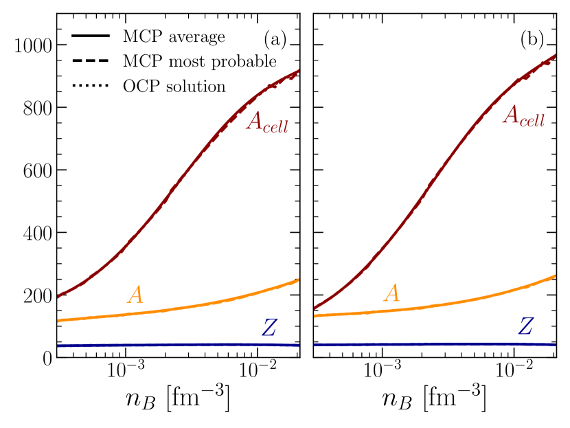
Figure 1: Variation with baryon density $n_{B}$ of the average (solid lines) and most probable (dashed lines) values of the charge number $Z$ (blue lines), cluster mass number $A$ (orange lines) and total mass number $A_{\rm cell}$ (red lines) in the inner crust at two selected temperatures: $T=10^{10}$ K (panel (a)), and $T=T_{\rm m}$ (panel (b)). Results obtained in the one-component plasma (OCP) approximation are also shown (dotted lines).

The average and most probable mass and charge number in the MCP are displayed in Fig. 1 as a function of the baryon density in the inner crust for $T=10^{10}$ K (panel (a)) and $T=T_{\rm m}$ (panel (b)). For comparison, the results obtained in the OCP approximation are also shown (dotted lines). We can see that the average and most probable values in the MCP approach follow very closely the OCP ones. This means that the deviations from the linear mixing rule in the liquid phase are small, as already noticed in Fantina et al. (2020) for the outer crust. While the mass numbers increase with density, the charge number is almost constant, $Z\approx 40$. The latter value is very close to that obtained at zero temperature (see also the dotted curve in Fig. 6, panel (b), in Carreau et al. (2020) and Fig. 12 in Pearson et al. (2018)), suggesting that the presence of $Z\approx 40$ ions in the inner crust is a robust result.

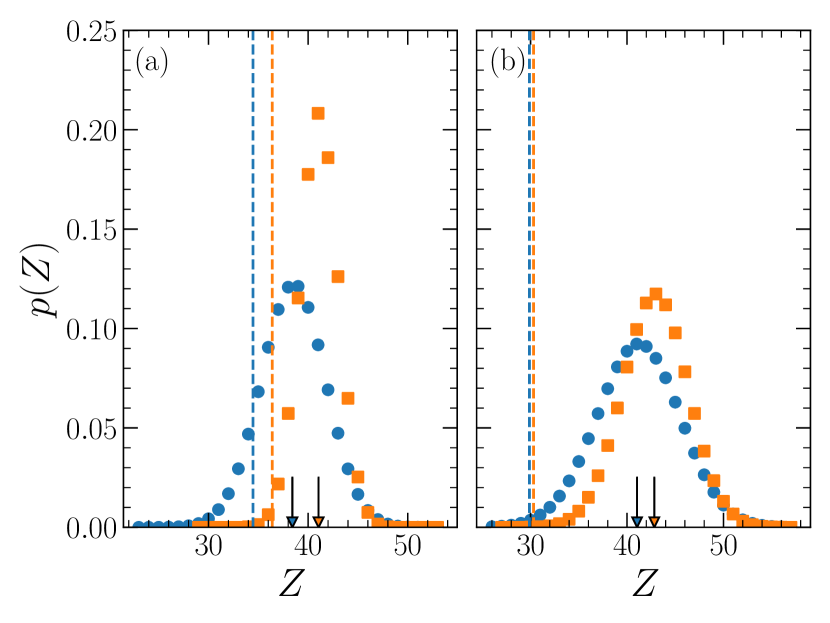
Figure 2: Normalized probability distribution $p(Z)$ for $n_{B}=5\times 10^{-4}$ fm^-3 (panel (a)) and $n_{B}=10^{-2}$ fm^-3 (panel (b)) at two selected temperatures: $T=10^{10}$ K (orange squares), and $T=T_{\rm m}$ (blue circles). Arrows indicate the OCP solutions. Vertical dashed lines correspond to the value of $\langle Z\rangle$ obtained without considering the rearrangement term (see text for details).

To evaluate the width of the distribution, we show in Fig. 2 the normalized probability distribution $p(Z)$ for $T=10^{10}$ K and $T=T_{\rm m}$ and for two selected densities in the inner crust: $n_{B}=5\times 10^{-4}$ fm^-3 (panel (a)) and $n_{B}=10^{-2}$ fm^-3 (panel (b)). The peaks of the distributions, i.e. the most probable $Z$, coincide with the charge numbers predicted in the OCP approximation (shown by the associated arrows), thus indicating that the linear mixing rule is a good approximation. To assess the importance of the rearrangement term, Eq. (47), we mark with vertical lines the average values of the charge number, $\langle Z\rangle$, obtained when this term is not included in the calculations. We observe that the effect of the rearrangement term is significant, particularly at higher density. Indeed, without taking into account this term, the distribution is systematically and considerably shifted towards lower $Z$, proving that the rearrangement term is actually needed to satisfy the thermodynamic consistency. We can also notice that, as expected, the distributions become broader with increasing temperature and density, thus making the OCP approximation less reliable. The flattening of the distribution is more clearly visible in Fig. 3 where the normalized probability distribution $p(Z)$ at the crystallization temperature is plotted for different increasing baryon densities in the inner crust. While the average value of $Z$ is centered around $40$ throughout the inner crust, the range of $Z$ of the distribution varies from $\approx 20$ closer to the neutron drip up to $\approx 40$ near the crust-core transition.

To better assess the evolution of the nuclear distribution, both in charge and mass number with density and temperature, we show in Fig. 4 the normalized probability distribution $p(Z,N)$ for two selected densities in the inner crust: $n_{B}=5\times 10^{-4}$ fm^-3 (panels (a) and (b)) and $n_{B}=10^{-2}$ fm^-3 (panels (c) and (d)), both at $T=10^{10}$ K (panels b and d) and $T=T_{\rm m}$ (panels (a) and (c)). As expected, going from lower to higher densities (upper to lower panels), we observe that the ions species become more neutron rich and that the distribution, both in $Z$ and $N$, broadens when going from lower to higher temperatures (left to right panels).

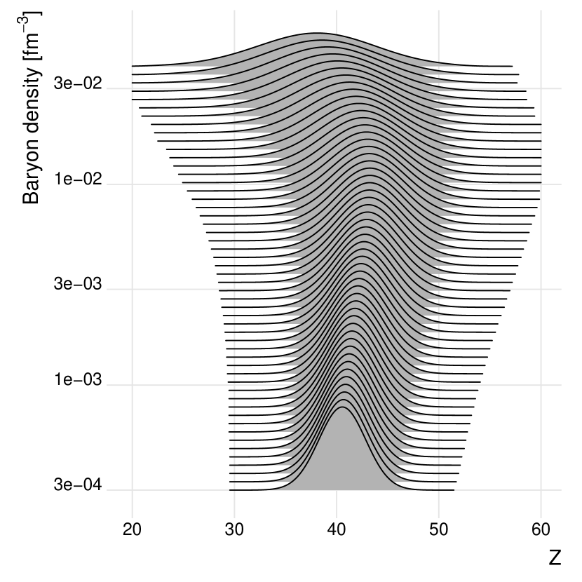
Figure 3: Normalized probability distribution $p(Z)$ with increasing baryon density $n_{B}$ in the inner crust at the crystallization temperature $T_{\rm m}$.

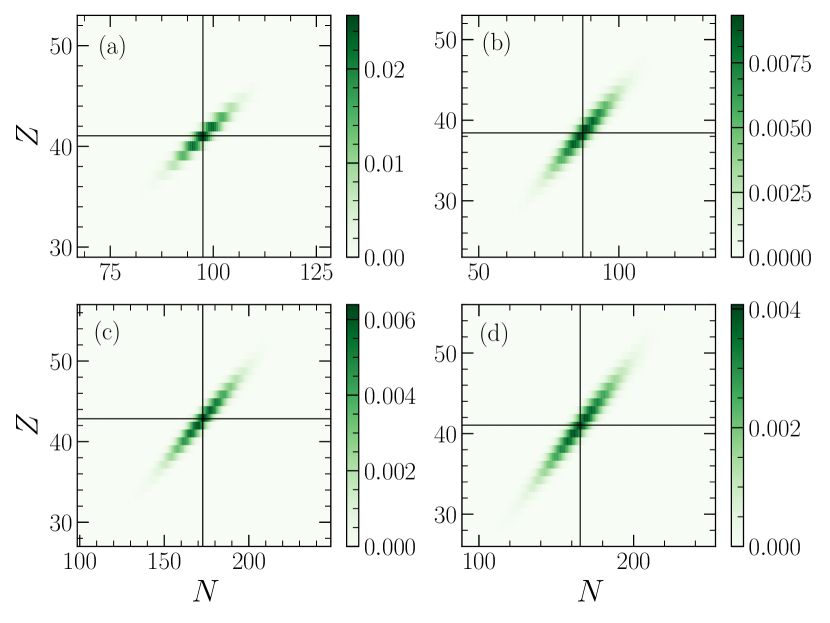
Figure 4: Normalized probability distribution of nuclei $p(N,Z)$ for four chosen thermodynamic conditions. Panel (a): $n_{B}=5\times 10^{-4}$ fm^-3, $T=T_{\rm m}$; Panel (b): $n_{B}=5\times 10^{-4}$ fm^-3, $T=10^{10}$ K; Panel (c): $n_{B}=10^{-2}$ fm^-3, $T=T_{\rm m}$; Panel (d): $n_{B}=10^{-2}$ fm^-3, $T=10^{10}$ K. In each panel, the OCP solution coincides with the intersection of the black lines.

3.2 Impurity parameter

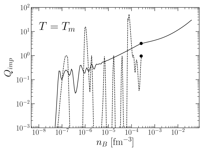
Figure 5: Variation with baryon density $n_{B}$ of the impurity parameter $Q_{\rm imp}$ in the crust at the crystallization temperature $T=T_{\rm m}$. In the outer crust regime, solid line (dashed line) represents the BSk24 CLD (HFB-24) prediction. In the inner crust regime, the impurity parameter is calculated in the CLD approximation. Points indicate the neutron-drip transition.

The impurity parameter at the crystallization temperature is shown in the whole crust in Fig. 5, as calculated with the BSk24 CLD model (solid line). The black dot marks the neutron drip point. We can see that the impurity parameter in the inner crust is higher than in the outer crust, meaning that the distribution is less peaked thus the OCP approximation is less reliable than in the outer crust. Indeed, larger values of $Q_{\rm imp}$ indicate more appreciable deviations from the OCP predictions. For comparison, we also plot the impurity parameter, taken from Fantina et al. (2020), calculated in the outer crust with the HFB-24 model (dashed line). The latter calculations show more prominent variations of $Q_{\rm imp}$ with respect to the CLD model calculations. This is due to the natural inclusion of shell effects in the fully microscopic calculations, that exhibit bimodal distributions around values of pressure, corresponding to the simultaneous presence of the two characteristic elements of adjacent layers (see Fig. 6 in Fantina et al. (2020)). These strong fluctuations are naturally smoothed out in the CLD model, because the nuclear functional varies continuously with $A$ and $Z$, and so does the probability. However, we can observe that the CLD calculation nicely interpolates the microscopic results, with an average impurity factor steadily increasing with the density and lying in the interval $Q_{\rm imp}\approx 0,1-2$. Going in the inner crust, neutrons drip out of the finite ion volume, and the associated shell effects naturally disappear (Chamel 2006). The inclusion of proton shell effects in the inner crust would require a formidable numerical investment which is much beyond the purpose of the paper. Moreover, it was suggested in Carreau et al. (2020) that these effects are small at the higher melting temperature of the inner crust, and that their effect on the observables is smaller than the uncertainty brought by our imperfect knowledge of the smooth part of the energy functional. For this reason shell effects were completely neglected in our study. We expect that a fully microscopic calculation would still present oscillations in $Q_{\rm imp}$ beyond the drip point, that these oscillations should be progressively damped going deeper in the star, and that our calculation can be taken as a smooth interpolation of that oscillating behavior.

To have a quantitative prediction of the impurity factor, the problem of model dependence has to be addressed. Apart from the modeling of finite temperature shell effects discussed above, the main source of uncertainty of the calculation comes from the choice of the nuclear functional. We show, in Fig. 6, the impurity parameter, Eq. (22), as a function of the baryon density in the inner crust, at the crystallization temperature $T_{\rm m}$ (solid line), for the four considered BSk CLD models. These data, as well as tables of the impurity parameter on a density-temperature grid for the four considered models, are available in tabular format at the CDS. Considering that the chosen models are believed to cover the main uncertainty on the nuclear equation of state at sub-saturation density (Pearson et al. 2018), we can take the spread of $Q_{\rm imp}$ values as obtained by the four calculations, as a reasonable estimation of the uncertainty on the impurity parameter. Since this latter represents the variance of the charge distribution, low values of $Q_{\rm imp}$ indicate that the distribution is quite peaked and thus that the OCP approach is a good approximation, as it can also be seen from Figs. 1 and 2, panel (a). The monotonic increase of the impurity parameter with density is also in accordance with Fig. 3, which clearly show the growth of the width of the charge distribution with increasing density. While at lower densities all the models predict similar values of the impurity parameter ($\lesssim 5$), at higher densities the spread among the models becomes larger, with the model associated to the lower (larger) symmetry energy coefficient at saturation having the larger (lower) $Q_{\rm imp}$. The same trend is observed at $T=10^{10}$ K (dashed lines in Fig. 6), although the hierarchy of the models is not preserved.

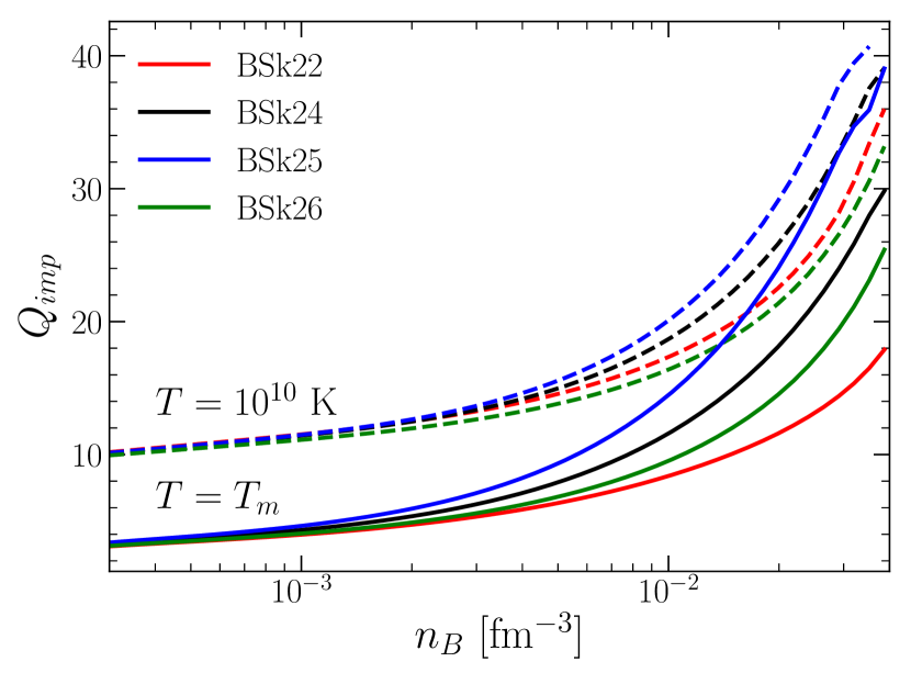
Figure 6: Variation with baryon density $n_{B}$ of the impurity parameter $Q_{\rm imp}$ in the inner crust regime at two selected temperatures: $T=10^{10}$ K, and $T=T_{\rm m}$, based on BSk22 (red lines), BSk24 (black lines), BSk25 (blue lines), and BSk26 (green lines) CLD calculations.

4 Conclusions

In this paper, we have presented a multi-component approach for the modeling of the crust of isolated unmagnetized NSs. Completing the work of Fantina et al. (2020) on the outer crust, the composition of the inner crust is evaluated with an extended nuclear statistical equilibrium based on a CLD model for the nuclear part of the ion energetics. To achieve thermodynamical consistency, a rearrangement term is explicitly worked out. This term has an important effect on the distributions and it is necessary to recover the correct limit at zero temperature. Since NSs are born hot, the equilibrium composition of a mature NS can be determined assuming a liquid phase for the MCP, at the lowest temperature at which strong and weak equilibrium are attained. In the absence of a dynamical estimation of the associated reaction rates, we consider the lowest temperature limit as given by the OCP crystallization temperature $T_{\rm m}$. We show that at that temperature the OCP approximation gives a very good estimation of the average composition of the inner crust, non-linear mixing terms playing a very small role in the liquid phase. However, an important contribution of impurities is obtained, favoring the picture of a temperature-independent high resistivity in the inner crust for all $T<T_{\rm m}$.

In order to reach quantitative predictions for the associated impurity parameter, we consider four different realistic microscopic nuclear functionals of the BSk family, which cover the present uncertainty in the nuclear modeling below the nuclear matter saturation density. The impurity parameter is seen to increase with the density, and values in the interval $Q_{\rm imp}\approx 20-40$ are reached at the highest densities considered in this study, namely $n_{B}=0.04$ fm^-3. Higher values of the impurity parameter might be expected in the deepest region of the inner crust, close to the core-crust transition, due to the presence of non-spherical pasta phases, which have not been considered in the present study.