Compositional Construction of Finite MDPs for Continuous-Time Stochastic Systems: A Dissipativity Approach

Abstract.

This paper provides a compositional scheme based on dissipativity approaches for constructing finite abstractions of continuous-time continuous-space stochastic control systems. The proposed framework enjoys the structure of the interconnection topology and employs a notion of stochastic storage functions, that describe joint dissipativity-type properties of subsystems and their abstractions. By utilizing those stochastic storage functions, one can establish a relation between continuous-time continuous-space stochastic systems and their finite counterparts while quantifying probabilistic distances between their output trajectories. Consequently, one can employ the finite system as a suitable substitution of the continuous-time one in the controller design process with a guaranteed error bound. In this respect, we first leverage dissipativity-type compositional conditions for the compositional quantification of the distance between the interconnection of continuous-time continuous-space stochastic systems and that of their discrete-time (finite or infinite) abstractions. We then consider a specific class of stochastic affine systems and construct their finite abstractions together with their corresponding stochastic storage functions. The effectiveness of the proposed results is demonstrated by applying them to a temperature regulation in a circular network containing $100$ rooms and compositionally constructing a discrete-time abstraction from its original continuous-time dynamic. The constructed discrete-time abstraction is then utilized as a substitute to compositionally synthesize policies keeping the temperature of each room in a comfort zone.

1. Introduction

Motivations. Automated controller synthesis for continuous-time continuous-space stochastic systems against high-level logical properties such as those expressed as linear temporal logic (LTL) formulae [Pnu77] is naturally a difficult task mainly due to continuous state sets. To deal with this problem, one potential direction is to first abstract the given system by a simpler one, i.e., discrete in time and potentially in space, then synthesize a desired controller for the abstract system, and finally transfer the controller back to the original one while quantifying probabilistic error bounds.

Unfortunately, curse of dimensionality is the main problem in the construction of finite abstractions (a.k.a. finite Markov decision processes (MDPs)) for large-scale systems: the complexity of constructing finite abstractions increases exponentially with the dimension of the state set. Compositional techniques play significant roles to alleviate this complexity. In this regard, one can consider the large-scale stochastic system as an interconnected system composed of several smaller subsystems, and then develop a compositional scheme for the construction of finite abstractions for the given complex system via abstractions of smaller subsystems.

Related Literature. There have been some results, proposed in the past few years, on the construction of finite abstractions for continuous-time continuous-space stochastic systems. A reachability analysis for continuous-time stochastic systems by constructing Markov chain with quantified error bounds is proposed in [LAB⁺17]. Abstraction approaches for incrementally stable stochastic control systems without discrete dynamics, incrementally stable stochastic switched systems, and randomly switched stochastic systems are respectively studied in [ZMEM⁺14], [ZAG15], and [ZA14]. Although original systems in [ZMEM⁺14], [ZAG15], and [ZA14] are stochastic, their abstractions are constructed as finite labeled transition systems while finite abstractions in this work are presented as finite Markov decision processes. Finite labeled transition systems in this context are useful only if the noise in the system is small. An approximation scheme for the construction of infinite abstractions for jump-diffusion processes is developed in [JP09]. Compositional construction of infinite abstractions via small-gain type conditions is proposed in [ZRME17]. An (in)finite abstraction-based technique for synthesis of continuous-time stochastic control systems is recently discussed in [NSZ19].

For discrete-time stochastic systems with continuous-state sets, there also exist several results. Finite abstractions for formal synthesis of discrete-time stochastic control systems are proposed in [APLS08]. An adaptive and sequential gridding approach is proposed in [Sou14], and [SA13] with dedicated tools FAUST² [SGA15] and StocHy [CA19]. Moreover, formal abstraction-based policy synthesis is discussed in [TMKA13], and [KSL13]. Compositional construction of infinite abstractions via classic small-gain and dissipativity conditions is respectively proposed in [LSMZ17, LSZ19b]. Compositional construction of finite abstractions utilizing dynamic Bayesian networks and dissipativity conditions is studied in [SAM17] and [LSZ18b], respectively. Although the proposed compositional approach in [LSZ18b] is based on dissipativity conditions, their results are provided for discrete-time systems. In comparison, we deal with continuous-time systems here and the ultimate goal is to develop a compositional approach to construct finite MDPs from continuous-time stochastic systems.

Compositional construction of (in)finite abstractions via $\max$-type small-gain conditions is proposed in [LSZ18a, LSZ20c]. Compositional construction of finite abstractions for networks of stochastic systems via relaxed small-gain and dissipativity approaches is respectively presented in [LSZ19c, LSZ20b]. A notion of approximate simulation relation for stochastic systems based on a lifting probabilistic evolution of systems is proposed in [HSA17]. This notion is generalized in [LSZ19a] for compositional abstraction-based synthesis of general MDPs. Compositional construction of finite abstractions for networks of stochastic switched systems accepting multiple Lyapunov functions with dwell-time conditions is presented in [LSZ20a, LZ19] via respectively small-gain and dissipativity approaches. Compositional construction of infinite and finite abstractions for large-scale discrete-time stochastic systems via different novel compositionality conditions is widely discussed in [Lav19].

Contributions. In this paper, we provide a compositional scheme for constructing finite MDPs from continuous-time continuous-space stochastic systems. We derive dissipativity-type conditions to propose compositionality results which are established based on relations between continuous-time subsystems and that of their abstract counterparts utilizing notions of so-called stochastic storage functions. The provided compositionality conditions can enjoy the structure of interconnection topology and be potentially fulfilled independently of the interconnection or gains of the subsystems (cf. the case study).

To this end, we first compositionally quantify the probabilistic distance between the interconnection of continuous-time continuous-space stochastic subsystems and their discrete-time (finite or infinite) abstractions. We then focus on a particular class of stochastic affine systems and construct their finite abstractions together with their corresponding stochastic storage functions. Finally, we illustrate the effectiveness of the proposed techniques by applying them to a physical case study.

Recent Works. Compositional abstraction-based synthesis of continuous-time stochastic systems is also proposed in [NSZ20], but using a different compositionality scheme based on small-gain conditions. Our proposed compositionality approach here can be potentially less conservative than the one presented in [NSZ20] for some classes of systems. The dissipativity-type compositional reasoning proposed here can enjoy the structure of the interconnection topology and may not require any constraint on the number or gains of subsystems (cf. Remark 4.4 and the case study). Consequently, the proposed approach here can provide a scale-free compositionality condition which is independent of the number of subsystems compared to the proposed results in [NSZ20].

2. Notations and Model Classes

2.1. Notations

A probability space in this work is defined as $(\Omega,\mathcal{F}_{\Omega},\mathds{P}_{\Omega})$, where $\Omega$ is the sample space, $\mathcal{F}_{\Omega}$ is a sigma-algebra on $\Omega$ comprising subsets of $\Omega$ as events, and $\mathds{P}_{\Omega}$ is a probability measure that assigns probabilities to events. We assume that triple $(\Omega,\mathcal{F}_{\Omega},\mathds{P}_{\Omega})$ denotes a probability space endowed with a filtration $\mathbb{F}=(\mathcal{F}_{s})_{s\geq 0}$ satisfying the usual conditions of completeness and right continuity.

Sets of nonnegative and positive integers are respectively denoted by $\mathbb{N}:=\{0,1,2,\ldots\}$ and $\mathbb{N}_{\geq 1}:=\{1,2,3,\ldots\}$. Symbols $\mathbb{R}$, $\mathbb{R}_{>0}$, and $\mathbb{R}_{\geq 0}$ respectively denote sets of real, positive and nonnegative real numbers. We use $x=[x_{1};\ldots;x_{N}]$ to denote the corresponding vector of dimension $\sum_{i}n_{i}$, given $N$ vectors $x_{i}\in\mathbb{R}^{n_{i}}$, $n_{i}\in\mathbb{N}_{\geq 1}$, and $i\in\{1,\ldots,N\}$. Given functions $f_{i}:X_{i}\rightarrow Y_{i}$, for any $i\in\{1,\ldots,N\}$, their Cartesian product $\prod_{i=1}^{N}f_{i}:\prod_{i=1}^{N}X_{i}\rightarrow\prod_{i=1}^{N}Y_{i}$ is defined as $(\prod_{i=1}^{N}f_{i})(x_{1},\ldots,x_{N})=[f_{1}(x_{1});\ldots;f_{N}(x_{N})]$. We denote by $\|\cdot\|$ the Euclidean norm. Given a function $f:\mathbb{N}\rightarrow\mathbb{R}^{n}$, the supremum of $f$ is denoted by $\|f\|_{\infty}:=\text{(ess)sup}\{\|f(k)\|,k\geq 0\}$. The identity matrix in $\mathbb{R}^{n\times{n}}$ is denoted by $\mathds{I}_{n}$. Column vectors in $\mathbb{R}^{n\times{1}}$ with all elements equal to zero and one are respectively denoted by $\mathbf{0}_{n}$ and $\mathds{1}_{n}$. A function $\gamma:\mathbb{\mathbb{missing}}\mathbb{R}_{\geq 0}\rightarrow\mathbb{\mathbb{missing}}\mathbb{R}_{\geq 0}$, is said to be a class $\mathcal{K}$ function if it is continuous, strictly increasing, and $\gamma(0)=0$. A class $\mathcal{K}$ function $\gamma(\cdot)$ is said to be a class $\mathcal{K}_{\infty}$ if $\gamma(s)\rightarrow\infty$ as $s\rightarrow\infty$.

2.2. Continuous-Time Stochastic Control Systems

Definition 2.1.

A continuous-time stochastic control system (ct-SCS) in this paper is defined by the tuple

$$\Sigma=(X,U,W,\mathcal{U},\mathcal{W},f,\sigma,Y_{1},Y_{2},h_{1},h_{2}),$$ (2.1)

where:

• $X\subseteq\mathbb{R}^{n}$ is the state set of the system;

• $U\subseteq\mathbb{R}^{m}$ is the external input set of the system;

• $W\subseteq\mathbb{R}^{p}$ is the internal input set of the system;

• $\mathcal{U}$ and $\mathcal{W}$ are subsets of the sets of all $\mathbb{F}$-progressively measurable processes taking values respectively in $\mathbb{R}^{m}$ and $\mathbb{R}^{p}$;

• $f:X\times U\times W\rightarrow X$ is the drift term which is globally Lipschitz continuous: there exist constants $\mathscr{L}_{x},\mathscr{L}_{\nu},\mathscr{L}_{w}\in\mathbb{R}_{\geq 0}$ such that $\|f(x,\nu,w)-f(x^{\prime},\nu^{\prime},w^{\prime})\|\leq\mathscr{L}_{x}\|x-x^{\prime}\|+\mathscr{L}_{\nu}\|\nu-\nu^{\prime}\|+\mathscr{L}_{w}\|w-w^{\prime}\|$ for all $x,x^{\prime}\in X$, for all $\nu,\nu^{\prime}\in U$, and for all $w,w^{\prime}\in W$;

• $\sigma:\mathbb{R}^{n}\rightarrow\mathbb{R}^{n\times\textsf{b}}$ is the diffusion term which is globally Lipschitz continuous with the Lipschitz constant $\mathscr{L}_{\sigma}$;

• $Y_{1}\subseteq\mathbb{R}^{q_{1}}$ is the external output set of the system;

• $Y_{2}\subseteq\mathbb{R}^{q_{2}}$ is the internal output set of the system;

• $h_{1}:X\rightarrow Y_{1}$ is the external output map;

• $h_{2}:X\rightarrow Y_{2}$ is the internal output map.

A continuous-time stochastic control system $\Sigma$ satisfies

$$\Sigma:\left\{\begin{array}[]{l}\mathsf{d}\xi(t)=f(\xi(t),\nu(t),w(t))\,\mathsf{d}t+\sigma(\xi(t))\,\mathsf{d}\mathbb{W}_{t},\\ \zeta_{1}(t)=h_{1}(\xi(t)),\\ \zeta_{2}(t)=h_{2}(\xi(t)),\\ \end{array}\right.$$ (2.5)

$\mathds{P}$-almost surely ($\mathds{P}$-a.s.) for any $\nu\in\mathcal{U}$ and $w\in\mathcal{W}$, where $(\mathbb{W}_{t})_{t\geq 0}$ is a b-dimensional Brownian motion, and stochastic processes $\xi:\Omega\times\mathbb{R}_{\geq 0}\rightarrow X$, $\zeta_{1}:\Omega\times\mathbb{R}_{\geq 0}\rightarrow Y_{1}$, and $\zeta_{2}:\Omega\times\mathbb{R}_{\geq 0}\rightarrow Y_{2}$ are respectively called the solution process and the external and internal output trajectories of $\Sigma$. We also use $\xi_{a\nu w}(t)$ to denote the value of the solution process at time $t\in\mathbb{R}_{\geq 0}$ under input trajectories $\nu$ and $w$ from an initial condition $\xi_{a\nu w}(0)=a$ $\mathds{P}$-a.s., where $a$ is a random variable that is $\mathcal{F}_{0}$-measurable. We also denote by $\zeta_{1_{a\nu w}}$ and $\zeta_{2_{a\nu w}}$ the external and internal output trajectories corresponding to the solution process $\xi_{a\nu w}$.

Remark 2.2.

Note that in this article, the term “internal” is used for inputs and outputs of subsystems that are affecting each other in the interconnection topology while properties of interest are defined over “external” outputs. The ultimate goal is to synthesize “external” inputs to fulfill desired properties over “external” outputs.

In this paper, we are interested in investigating interconnected continuous-time stochastic systems, defined later in Subsection 4.1, without internal signals. Then the tuple (2.1) reduces to $(X,U,\mathcal{U},f,\sigma,Y,h)$ with $f:X\times U\rightarrow X$, and ct-SCS (2.5) can be re-written as

$$\Sigma:\left\{\begin{array}[]{l}\mathsf{d}\xi(t)=f(\xi(t),\nu(t))\,\mathsf{d}t+\sigma(\xi(t))\,\mathsf{d}\mathbb{W}_{t},\\ \zeta(t)=h(\xi(t)).\\ \end{array}\right.$$ (2.8)

2.3. Finite Abstractions of ct-SCS

In order to construct finite abstractions of continuous-time stochastic systems, we first need to provide a time-discretized version of ct-SCS in (2.5) as in the following definition.

Definition 2.3.

A time-discretized version of ct-SCS $\Sigma$ is defined by the tuple

$$\widetilde{\Sigma}=\left(\tilde{X},\tilde{U},\tilde{W},\varsigma,\tilde{f},\tilde{Y}_{1},\tilde{Y}_{2},\tilde{h}_{1},\tilde{h}_{2}\right)\!,$$ (2.9)

where:

• $\tilde{X}\subseteq\mathbb{R}^{n}$ is a Borel space as the state set of the system. We denote by $(\tilde{X},\mathcal{B}(\tilde{X}))$ the measurable space with $\mathcal{B}(\tilde{X})$ being the Borel sigma-algebra on the state space;

• $\tilde{U}\subseteq\mathbb{R}^{m}$ is a Borel space as the external input set;

• $\tilde{W}\subseteq\mathbb{R}^{p}$ is a Borel space as the internal input set;

• $\varsigma$ is a sequence of independent and identically distributed (i.i.d.) random variables from a sample space $\Omega$ to the set $\mathcal{V}_{\varsigma}$,

  $$\varsigma:=\{\varsigma(k):\Omega\rightarrow\mathcal{V}_{\varsigma},\,\,k\in\mathbb{N}\};$$

• $\tilde{f}:\tilde{X}\times\tilde{U}\times\tilde{W}\times\mathcal{V}_{\varsigma}\rightarrow\tilde{X}$ is a measurable function characterizing the state evolution of the system;

• $\tilde{Y}_{1}\subseteq\mathbb{R}^{q_{1}}$ is a Borel space as the external output set;

• $\tilde{Y}_{2}\subseteq\mathbb{R}^{q_{2}}$ is a Borel space as the internal output set;

• $\tilde{h}_{1}:\tilde{X}\rightarrow\tilde{Y}_{1}$ is the external output map;

• $\tilde{h}_{2}:\tilde{X}\rightarrow\tilde{Y}_{2}$ is the internal output map.

The evolution of $\widetilde{\Sigma}$, for given initial state $\tilde{x}(0)\in\tilde{X}$ and input sequences $\{\tilde{\nu}(k):\Omega\rightarrow\tilde{U},\,\,k\in\mathbb{N}\}$ and $\{\tilde{w}(k):\Omega\rightarrow\tilde{W},\,\,k\in\mathbb{N}\}$, can be written as

$$\widetilde{\Sigma}:\left\{\begin{array}[]{l}\tilde{\xi}(k+1)=\tilde{f}(\tilde{\xi}(k),\tilde{\nu}(k),\tilde{w}(k),\varsigma(k)),\\ \tilde{\zeta}_{1}(k)=\tilde{h}_{1}(\tilde{\xi}(k)),\\ \tilde{\zeta}_{2}(k)=\tilde{h}_{2}(\tilde{\xi}(k)),\\ \end{array}\right.k\in\mathbb{N}.$$ (2.13)

The sets $\mathcal{\tilde{U}}$ and $\mathcal{\tilde{W}}$ are associated to $\tilde{U}$ and $\tilde{W}$ to be the collections of sequences $\{\tilde{\nu}(k):\Omega\rightarrow\tilde{U},\,\,k\in\mathbb{N}\}$ and $\{\tilde{w}(k):\Omega\rightarrow\tilde{W},\,\,k\in\mathbb{N}\}$, in which $\tilde{\nu}(k)$ and $\tilde{w}(k)$ are independent of $\varsigma(z)$ for any $k,z\in\mathbb{N}$ and $z\geq k$. For any initial state $\tilde{a}\in\tilde{X}$, $\tilde{\nu}(\cdot)\in\mathcal{\tilde{U}}$ and $\tilde{w}(\cdot)\in\mathcal{\tilde{W}}$, the random sequences $\tilde{\xi}_{\tilde{a}\tilde{\nu}\tilde{w}}:\Omega\times\mathbb{N}\rightarrow\tilde{X}$, $\tilde{\zeta}_{1_{\tilde{a}\tilde{\nu}\tilde{w}}}:\Omega\times\mathbb{N}\rightarrow\tilde{Y}_{1}$, and $\tilde{\zeta}_{2_{\tilde{a}\tilde{\nu}\tilde{w}}}:\Omega\times\mathbb{N}\rightarrow\tilde{Y}_{2}$ fulfilling (2.13) are respectively called the solution process, and external and internal output trajectories of $\widetilde{\Sigma}$ under an external input $\tilde{\nu}$, an internal input $\tilde{w}$, and an initial state $\tilde{a}$.

Remark 2.4.

Note that the discrete-time system $\tilde{\Sigma}$ in (2.13) is presented independently of ct-SCS $\Sigma$ for now. In particular, in order to construct finite abstractions of continuous-time stochastic systems $\Sigma$ (i.e., $\widehat{\Sigma}$) as proposed in Definition 2.6, one first needs to provide a time-discretized version of ct-SCS (i.e., $\widetilde{\Sigma}$) as a middle stage. In Section 5, we focus on a particular class of continuous-time stochastic affine systems $\Sigma$ and discuss the best choice for $\widetilde{\Sigma}$ to acquire the least approximation error between $\Sigma$ and $\widehat{\Sigma}$.

The discrete-time stochastic control system $\widetilde{\Sigma}$ can be equivalently reformulated as a Markov decision process [Kal97, Proposition 7.6]

$$\widetilde{\Sigma}=\left(\tilde{X},\tilde{U},\tilde{W},\tilde{T}_{\mathsf{\tilde{x}}},\tilde{Y}_{1},\tilde{Y}_{2},\tilde{h}_{1},\tilde{h}_{2}\right)\!,$$

where the map $\tilde{T}_{\mathsf{\tilde{x}}}:\mathcal{B}(\tilde{X})\times\tilde{X}\times\tilde{U}\times\tilde{W}\rightarrow[0,1]$, is a conditional stochastic kernel that assigns to any $\tilde{x}\in\tilde{X}$, $\tilde{\nu}\in\tilde{U}$, and $\tilde{w}\in\tilde{W}$, a probability measure $\tilde{T}_{\mathsf{\tilde{x}}}(\cdot|\tilde{x},\tilde{\nu},\tilde{w})$ on the measurable space $(\tilde{X},\mathcal{B}(\tilde{X}))$ so that for any set $\mathcal{A}\in\mathcal{B}(\tilde{X})$,

$$\mathds{P}(\tilde{x}(k+1)\in\mathcal{A}\,\big{|}\,\tilde{x}(k),\tilde{\nu}(k),\tilde{w}(k))= \int_{\mathcal{A}}\tilde{T}_{\mathsf{\tilde{x}}}(\mathsf{d}\tilde{x}(k+1)\,\big{|}\,\tilde{x}(k),\tilde{\nu}(k),\tilde{w}(k)).$$

For given inputs $\tilde{\nu}(\cdot),\tilde{w}(\cdot),$ the stochastic kernel $\tilde{T}_{\mathsf{\tilde{x}}}$ captures the evolution of the state of $\widetilde{\Sigma}$ and can be uniquely specified by the pair $(\varsigma,\tilde{f})$ from (2.9). We now define Markov policies in order to control the system.

Definition 2.5.

For the discrete-time stochastic control system $\widetilde{\Sigma}$ in (2.13), a Markov policy is a sequence $\bar{\mu}=(\bar{\mu}_{0},\bar{\mu}_{1},\bar{\mu}_{2},\ldots)$ of universally measurable stochastic kernels $\bar{\mu}_{n}$ [BS96], each defined on the input space $\tilde{U}$ given $\tilde{X}\times\tilde{W}$ such that for all $(\tilde{\xi}_{n},\tilde{w}_{n})\in\tilde{X}\times\tilde{W}$, $\bar{\mu}_{n}(\tilde{U}|(\tilde{\xi}_{n},\tilde{w}_{n}))=1$. The class of all such Markov policies is denoted by $\mathcal{P}_{\mathcal{M}}$.

Now we construct finite MDPs $\widehat{\Sigma}$ as finite abstractions of discrete-time stochastic systems $\widetilde{\Sigma}$ in (2.13). The abstraction algorithm is based on finite partitions of sets $\tilde{X}=\cup_{i}\mathsf{X}_{i}$, $\tilde{U}=\cup_{i}\mathsf{U}_{i}$, and $\tilde{W}=\cup_{i}\mathsf{W}_{i}$ and the selection of representative points $\bar{\xi}_{i}\in\mathsf{X}_{i}$, $\bar{\nu}_{i}\in\mathsf{U}_{i}$, and $\bar{w}_{i}\in\mathsf{W}_{i}$ as abstract states and inputs as formalized in the following definition.

Definition 2.6.

Given a discrete-time system $\widetilde{\Sigma}=(\tilde{X},\tilde{U},\tilde{W},$ $\varsigma,\tilde{f},\tilde{Y}_{1},\tilde{Y}_{2},\tilde{h}_{1},\tilde{h}_{2})$, its finite abstraction $\widehat{\Sigma}$ can be characterized as

$$\widehat{\Sigma}=(\hat{X},\hat{U},\hat{W},\varsigma,\hat{f},\hat{Y}_{1},\hat{Y}_{2},\hat{h}_{1},\hat{h}_{2}),$$ (2.14)

where $\hat{X}=\{\bar{\xi}_{i},i=1,\ldots,n_{\tilde{\xi}}\}$, $\hat{U}=\{\bar{\nu}_{i},i=1,\ldots,n_{\tilde{\nu}}\}$, and $\hat{W}=\{\bar{w}_{i},i=1,\ldots,n_{\tilde{w}}\}$ are sets of selected representative points. Function $\hat{f}:\hat{X}\times\hat{U}\times\hat{W}\times\mathcal{V}_{\varsigma}\rightarrow\hat{X}$ is defined as

$$\hat{f}(\hat{\xi},\hat{\nu},\hat{w},\varsigma)=\Pi_{\tilde{\xi}}(\tilde{f}(\hat{\xi},\hat{\nu},\hat{w},\varsigma)),$$ (2.15)

where $\Pi_{\tilde{\xi}}:\tilde{X}\rightarrow\hat{X}$ is a map that assigns to any $\tilde{\xi}\in\tilde{X}$, the representative point $\bar{\xi}\in\hat{X}$ of the corresponding partition set containing $\tilde{\xi}$. The output maps $\hat{h}_{1}$, $\hat{h}_{2}$ are the same as $\tilde{h}_{1}$, $\tilde{h}_{2}$ with their domain restricted to the finite state set $\hat{X}$ and the output sets $\hat{Y}_{1}$, $\hat{Y}_{2}$ are just the image of $\hat{X}$ under $\tilde{h}_{1}$, $\tilde{h}_{2}$. The initial state of $\widehat{\Sigma}$ is also selected according to $\hat{\xi}_{0}:=\Pi_{\tilde{\xi}}(\tilde{\xi}_{0})$ with $\tilde{\xi}_{0}$ being the initial state of $\widetilde{\Sigma}$.

The abstraction map $\Pi_{\tilde{\xi}}$ defined in (2.15) satisfies the inequality

$$\|\Pi_{\tilde{\xi}}(\tilde{\xi})-\tilde{\xi}\|\leq\delta,\leavevmode\nobreak\ \quad\forall\tilde{\xi}\,\in\tilde{X},$$ (2.16)

where $\delta$ is the state discretization parameter defined as $\delta:=\sup\{\|\tilde{\xi}-\tilde{\xi}^{\prime}\|,\,\,\tilde{\xi},\tilde{\xi}^{\prime}\in\mathsf{X}_{i},\,i=1,2,\ldots,n_{\tilde{\xi}}\}$.

Remark 2.7.

Note that to construct finite abstractions as in Definition 2.6, we assume the state and input sets of the discrete-time system $\widetilde{\Sigma}$ are restricted to compact regions.

3. Stochastic Storage and Simulation Functions

In this section, we first define a notion of stochastic storage functions (SStF) for ct-SCS with both internal and external signals. We then define a notion of stochastic simulation functions (SSF) for ct-SCS with only external signals. We utilize these two definitions to quantify the probabilistic closeness of interconnected continuous-time stochastic systems and that of their discrete-time (finite or infinite) abstractions.

Definition 3.1.

Consider a ct-SCS $\Sigma=(X,U,W,\mathcal{U},\mathcal{W},f,\sigma,Y_{1},Y_{2},h_{1},h_{2})$ and its (in)finite abstraction $\widehat{\Sigma}=(\hat{X},\hat{U},\hat{W},\varsigma,\hat{f},\hat{Y}_{1},\hat{Y}_{2},\hat{h}_{1},\hat{h}_{2})$. A function $S:X\times\hat{X}\to\mathbb{R}_{\geq 0}$ is called a stochastic storage function (SStF) from $\widehat{\Sigma}$ to $\Sigma$ if

• $\exists\alpha\in\mathcal{K}_{\infty}$ such that

  $$\forall x\in X,\forall\hat{x}\in\hat{X},\leavevmode\nobreak\ \leavevmode\nobreak\ \alpha(\|h_{1}(x)-\hat{h}_{1}(\hat{x})\|)\leq S(x,\hat{x}),$$ (3.1)

• $\forall k\in\mathbb{N}$, $\forall\xi:=\xi(k\tau)\in X,\forall\hat{\xi}:=\hat{\xi}(k)\in\hat{X}$, and $\forall\hat{\nu}:=\hat{\nu}(k)\in\hat{U}$, $\forall w:=w(k\tau)\in W$, $\forall\hat{w}:=\hat{w}(k)\in\hat{W}$, $\exists\nu:=\nu(k\tau)\in U$ such that

  $$\mathds{E} \Big{[}S(\xi((k+1)\tau),\hat{\xi}(k+1))\,\big{|}\,\xi,\hat{\xi},\nu,\hat{\nu},w,\hat{w}\Big{]}$$ (3.2)

  $$\leq\kappa S(\xi,\hat{\xi})+\rho_{\mathrm{ext}}(\|\hat{\nu}\|)+\psi+\begin{bmatrix}w-\hat{w}\\ h_{2}(x)-\hat{h}_{2}(\hat{x})\end{bmatrix}^{T}\underbrace{\begin{bmatrix}\bar{X}^{11}&\bar{X}^{12}\\ \bar{X}^{21}&\bar{X}^{22}\end{bmatrix}}_{\bar{X}:=}\begin{bmatrix}w-\hat{w}\\ h_{2}(x)-\hat{h}_{2}(\hat{x})\end{bmatrix}\!\!,$$

  for some chosen sampling time $\tau\in\mathbb{R}_{>0}$, $0<\kappa<1$, $\rho_{\mathrm{ext}}\in\mathcal{K}_{\infty}$, $\psi\in{\mathbb{R}}_{>0}$, and a symmetric matrix $\bar{X}$ with conformal block partitions $\bar{X}^{ij}$, $i,j\in\{1,2\}$.

We call the control system $\widehat{\Sigma}$ a discrete-time (in)finite abstraction of concrete (original) system $\Sigma$ if there exists an SStF $S$ from $\widehat{\Sigma}$ to $\Sigma$. Abstraction $\widehat{\Sigma}$ could be finite or infinite depending on cardinalities of sets $\hat{X},\hat{U},\hat{W}$. Since the above definition does not put any restriction on the state set of abstract systems, it can be also used to define a stochastic storage function from discrete-time system $\widetilde{\Sigma}$ presented in (2.9) to $\Sigma$ (cf. the case study).

Remark 3.2.

Note that one can rewrite the left-hand side of (3.2) using Dynkin’s formula [Dyn65] as

$$\mathds{E} \Big{[}S(\xi((k+1)\tau),\hat{\xi}(k+1))\,\big{|}\,\xi(k\tau),\hat{\xi}(k),\nu(k\tau),\hat{\nu}(k),w(k\tau),\hat{w}(k)\Big{]}$$

$$=\mathds{E}_{\varsigma}\Big{[}S(\xi(k\tau),\hat{\xi}(k+1))+\mathds{E}\Big{[}\int_{k\tau}^{(k+1)\tau}\mathcal{L}S(\xi(t),\hat{\xi}(k+1))\mathsf{d}t\Big{]}\,\big{|}\,\hat{\xi}(k),\hat{\nu}(k),\hat{w}(k)\Big{]}\!,$$

where $\mathcal{L}S$ is the infinitesimal generator of the stochastic process applying on the function $S$, and $\mathds{E}_{\varsigma}$ is the conditional expectation acting only on the noise of the abstract system. The above Dynkin’s formula is utilized later in Section 5 to show the results of Theorem 5.5.

Now, we write the above notion for the interconnected ct-SCS as the following definition.

Definition 3.3.

Consider a ct-SCS $\Sigma=(X,U,\mathcal{U},f,\sigma,Y,h)$ and its finite abstraction $\widehat{\Sigma}=(\hat{X},\hat{U},\varsigma,\hat{f},\hat{Y},\hat{h})$ without internal signals. A function $V:X\times\hat{X}\to\mathbb{R}_{\geq 0}$ is called a stochastic simulation function (SSF) from $\widehat{\Sigma}$ to $\Sigma$ if

• $\exists\alpha\in\mathcal{K}_{\infty}$ such that $\forall x\in X,\forall\hat{x}\in\hat{X},$ one has

  $$\alpha(\|h(x)-\hat{h}(\hat{x})\|)\leq V(x,\hat{x}),$$ (3.3)

• $\forall k\in\mathbb{N}$, $\forall\xi:=\xi(k\tau)\in X,\forall\hat{\xi}:=\hat{\xi}(k)\in\hat{X}$, and $\forall\hat{\nu}:=\hat{\nu}(k)\in\hat{U}$, $\exists\nu:=\nu(k\tau)\in U$ such that

  $$\mathds{E}\Big{[}V(\xi((k+1)\tau),\hat{\xi}(k+1))\,\big{|}\,\xi,\hat{\xi},\nu,\hat{\nu}\Big{]}\leq\kappa V(\xi,\hat{\xi})+\rho_{\mathrm{ext}}(\|\hat{\nu}\|)+\psi,$$ (3.4)

  for some chosen sampling time $\tau\in\mathbb{R}_{>0}$, $0<\kappa<1$, $\rho_{\mathrm{ext}}\in\mathcal{K}_{\infty}$, and $\psi\in\mathbb{R}_{>0}$.

The next theorem is borrowed from [LSMZ17, Theorem 3.3] and shows how SSF can be useful in providing the probabilistic closeness between output trajectories of original interconnected continuous-time stochastic systems and that of their discrete-time (finite or infinite) abstractions.

Theorem 3.4.

Let $\Sigma=(X,U,\mathcal{U},f,\sigma,Y,h)$ be a ct-SCS and $\widehat{\Sigma}=(\hat{X},\hat{U},\varsigma,\hat{f},\hat{Y},\hat{h})$ its discrete-time abstraction. Suppose $V$ is an SSF from $\widehat{\Sigma}$ to $\Sigma$. For any input trajectory $\hat{\nu}(\cdot)\in\mathcal{\hat{U}}$ that preserves Markov property for the closed-loop $\widehat{\Sigma}$, and for any random variables $a$ and $\hat{a}$ as initial states of the ct-SCS and its discrete-time abstraction, there exists an input trajectory $\nu(\cdot)\in\mathcal{U}$ of $\Sigma$ such that the following inequality holds over the finite-time horizon $T_{d}$:

$$\mathds{P} \left\{\sup_{0\leq k\leq T_{d}}\|\zeta_{a\nu}(k\tau)-\hat{\zeta}_{\hat{a}\hat{\nu}}(k)\|\geq\varepsilon\,|\,a,\hat{a}\right\}$$ (3.5)

$$\leq\begin{cases}1-(1-\frac{V(a,\hat{a})}{\alpha\left(\varepsilon\right)})(1-\frac{\hat{\psi}}{\alpha\left(\varepsilon\right)})^{T_{d}},&\quad\quad\text{if}\leavevmode\nobreak\ \alpha\left(\varepsilon\right)\geq\frac{\hat{\psi}}{\kappa},\\ (\frac{V(a,\hat{a})}{\alpha\left(\varepsilon\right)})(1-\kappa)^{T_{d}}+(\frac{\hat{\psi}}{\kappa\alpha\left(\varepsilon\right)})(1-(1-\kappa)^{T_{d}}),&\quad\quad\text{if}\leavevmode\nobreak\ \alpha\left(\varepsilon\right)<\frac{\hat{\psi}}{\kappa},\end{cases}$$

where $\hat{\psi}>0$ satisfies $\hat{\psi}\geq\rho_{\mathrm{ext}}(\|\hat{\nu}\|_{\infty})+\psi$.

4. Compositional Abstractions for Interconnected Systems

In this section, we analyze networks of stochastic control subsystems, $i\in\{1,\dots,N\},$

$$\Sigma_{i}=(X_{i},U_{i},W_{i},\mathcal{U}_{i},\mathcal{W}_{i},f_{i},\sigma_{i},Y_{1_{i}},Y_{2_{i}},h_{1_{i}},h_{2_{i}}),$$ (4.1)

and discuss how to construct their finite abstractions together with an SSF based on corresponding SStF of their subsystems.

4.1. Interconnected Stochastic Control Systems

We first formally define the interconnected stochastic control systems.

Definition 4.1.

Consider $N\!\in\!{\mathbb{N}}_{\geq 1}$ stochastic control subsystems $\Sigma_{i}\!=\!(X_{i},U_{i},W_{i},\mathcal{U}_{i},\mathcal{W}_{i},f_{i},\sigma_{i},Y_{1_{i}},Y_{2_{i}},\!h_{1_{i}},\!h_{2_{i}}\!)$, $i\in\{1,\dots,N\}$, and a matrix $M$ defining the coupling between these subsystems. We require the condition $M\prod_{i=1}^{N}Y_{2i}\subseteq\prod_{i=1}^{N}W_{i}$ to establish a well-posed interconnection. The interconnection of $\Sigma_{i}$, $\forall i\in\{1,\ldots,N\}$, is the ct-SCS $\Sigma=(X,U,\mathcal{U},f,\sigma,Y,h)$, denoted by $\mathcal{I}(\Sigma_{1},\ldots,\Sigma_{N})$, such that $X:=\prod_{i=1}^{N}X_{i}$, $U:=\prod_{i=1}^{N}U_{i}$, $f:=\prod_{i=1}^{N}f_{i}$, $\sigma:=[\sigma_{1}(x_{1});\cdots;\sigma_{N}(x_{N})]$, $Y:=\prod_{i=1}^{N}Y_{1i}$, and $h=\prod_{i=1}^{N}h_{1i}$, with the internal inputs constrained according to:

$${\left[w_{1};\cdots;w_{N}\right]}=M{\left[h_{21}(x_{1});\cdots;h_{2N}(x_{N})\right]}.$$

Remark 4.2.

Note that we do not have any restrictions on the interconnected matrix $M$ and its entries can take any values depending on the forms of interconnection topologies.

4.2. Compositional Abstractions of Interconnected Systems

We consider $\Sigma_{i}\!=\!(X_{i},U_{i},W_{i},\mathcal{U}_{i},\mathcal{W}_{i},f_{i},\\ \sigma_{i},Y_{1_{i}},Y_{2_{i}},h_{1_{i}},h_{2_{i}})$ as an original ct-SCS and $\widehat{\Sigma}_{i}$ as its discrete-time finite abstraction given by the tuple $\widehat{\Sigma}_{i}=(\hat{X}_{i},\hat{U}_{i},\hat{W}_{i},\varsigma_{i},\hat{f}_{i},\hat{Y}_{1_{i}},\hat{Y}_{2_{i}},\hat{h}_{1_{i}},\hat{h}_{2_{i}})$. We also assume that there exist an SStF $S_{i}$ from $\widehat{\Sigma}_{i}$ to $\Sigma_{i}$ with the corresponding functions, constants, and matrices denoted by $\alpha_{i}$, $\rho_{\text{ext}i}$, $\kappa_{i}$, $\psi_{i}$, $\bar{X}_{i}$, $\bar{X}_{i}^{11}$, $\bar{X}_{i}^{12}$, $\bar{X}_{i}^{21}$, and $\bar{X}_{i}^{22}$. In the next theorem, we quantify the error between the interconnection of continuous-time stochastic subsystems and that of their discrete-time abstractions in a compositional fashion.

Theorem 4.3.

Consider an interconnected stochastic control system $\Sigma=\mathcal{I}(\Sigma_{1},\ldots,\Sigma_{N})$ induced by $N\in{{\mathbb{N}}_{\geq 1}}$ stochastic control subsystems $\Sigma_{i}$ and the coupling matrix $M$. Let each subsystem $\Sigma_{i}$ admit an abstraction $\widehat{\Sigma}_{i}$ with the corresponding SStF $S_{i}$. Then

$$V(x,\hat{x}):=\sum_{i=1}^{N}\mu_{i}S_{i}(x_{i},\hat{x}_{i}),$$ (4.2)

is a stochastic simulation function from the interconnected system $\widehat{\Sigma}=\mathcal{I}(\widehat{\Sigma}_{1},\ldots,\widehat{\Sigma}_{N})$, with coupling matrix $\hat{M}$, to $\Sigma=\mathcal{I}(\Sigma_{1},\ldots,\Sigma_{N})$ if there exist $\mu_{i}>0$, $i\in\{1,\ldots,N\}$, and

$$\begin{bmatrix}M\\ \mathds{I}_{\tilde{q}}\end{bmatrix}^{T} \bar{X}_{cmp}\begin{bmatrix}M\\ \mathds{I}_{\tilde{q}}\end{bmatrix}\preceq 0,$$ (4.3)

$$M =\hat{M},$$ (4.4)

$$\hat{M}\prod_{i=1}^{N}\hat{Y}_{2i} \subseteq\prod_{i=1}^{N}\hat{W}_{i},$$ (4.5)

where

$$\bar{X}_{cmp}:=\begin{bmatrix}\mu_{1}\bar{X}_{1}^{11}&&&\mu_{1}\bar{X}_{1}^{12}&&\\ &\ddots&&&\ddots&\\ &&\mu_{N}\bar{X}_{N}^{11}&&&\mu_{N}\bar{X}_{N}^{12}\\ \mu_{1}\bar{X}_{1}^{21}&&&\mu_{1}\bar{X}_{1}^{22}&&\\ &\ddots&&&\ddots&\\ &&\mu_{N}\bar{X}_{N}^{21}&&&\mu_{N}\bar{X}_{N}^{22}\end{bmatrix}\!\!,\\$$ (4.6)

and $\tilde{q}=\sum_{i=1}^{N}q_{2i}$ with $q_{2i}$ being dimensions of the internal output of subsystems $\Sigma_{i}$.

Remark 4.4.

Condition (4.3) is similar to the LMI discussed in [AMP16] as a compositional stability condition based on the dissipativity theory. It is shown in [AMP16] that this condition holds independently of the number of subsystems in many physical applications with particular interconnection structures, e.g., skew symmetric.

5. Construction of Stochastic Storage Functions for a Class of Systems

In this section, we focus on a special class of continuous-time stochastic affine systems and impose conditions enabling us to establish an SStF from its finite abstraction $\widehat{\Sigma}$ to $\Sigma$. The model of the system is given by

$$\Sigma:\left\{\begin{array}[]{l}\mathsf{d}\xi(t)=(A\xi(t)+B\nu(t)+Dw(t)+\mathbf{b})\mathsf{d}t+G\mathsf{d}W_{t},\\ \zeta_{1}(t)=C_{1}\xi(t),\\ \zeta_{2}(t)=C_{2}\xi(t),\\ \end{array}\right.$$ (5.4)

where $A\in\mathbb{R}^{n\times n},B\in\mathbb{R}^{n\times m},D\in\mathbb{R}^{n\times p},C_{1}\in\mathbb{R}^{q_{1}\times n},C_{2}\in\mathbb{R}^{q_{2}\times n}$, $G\in\mathbb{R}^{n}$, and $\mathbf{b}\in\mathbb{R}^{n}$. We employ the tuple

$$\Sigma=(A,B,C_{1},C_{2},D,G,\mathbf{b}),$$

to refer to the class of stochastic affine systems in (5.4). The time-discretized version of $\Sigma$ is proposed as

$$\widetilde{\Sigma}:\left\{\begin{array}[]{l}\tilde{\xi}(k+1)=\tilde{\xi}(k)+\tilde{\nu}(k)+\tilde{D}\tilde{w}(k)+\tilde{R}\varsigma(k),\\ \tilde{\zeta}_{1}(k)=\tilde{C}_{1}\tilde{\xi}(k),\\ \tilde{\zeta}_{2}(k)=\tilde{C}_{2}\tilde{\xi}(k),\\ \end{array}\right.\quad k\in\mathbb{N},$$ (5.8)

where $\tilde{D}$ and $\tilde{R}$ are matrices chosen arbitrarily, and $\tilde{C}_{1}=C_{1}P$, $\tilde{C}_{2}=C_{2}P$ with $P$ as chosen in (5.13) (cf. Theorem 5.5). Our main target here is to employ $\widetilde{\Sigma}$ as the discrete-time version of $\Sigma$ in order to establish an SStF from $\widehat{\Sigma}$ to $\Sigma$ through $\widetilde{\Sigma}$ while quantifying the best approximation error. Later, in Remark 5.6, we show that $\tilde{R}=\mathbf{0}_{n}$ and $\tilde{D}=\mathbf{0}_{n\times p}$ result in the least approximation error in our settings. Now, we describe the finite abstraction of $\widetilde{\Sigma}$ as

$$\widehat{\Sigma}:\left\{\begin{array}[]{l}\hat{\xi}(k+1)=\Pi_{\tilde{\xi}}(\hat{\xi}(k)+\hat{\nu}(k)+\tilde{D}\hat{w}(k)+\tilde{R}\varsigma(k)),\\ \hat{\zeta}_{1}(k)=\hat{C}_{1}\hat{\xi}(k),\\ \hat{\zeta}_{2}(k)=\hat{C}_{2}\hat{\xi}(k),\\ \end{array}\right.\quad k\in\mathbb{N},$$ (5.12)

where map $\Pi_{\tilde{\xi}}:\tilde{X}\rightarrow\hat{X}$ satisfies the inequality (2.16). Now we candidate the following quadratic stochastic storage function

$$S(x,\hat{x})=(x-P\hat{x})^{T}\mathcal{\bar{M}}(x-P\hat{x}),$$ (5.13)

where $P$ is a square matrix and $\mathcal{\bar{M}}$ is a positive-definite matrix of an appropriate dimension. In order to show that $S$ in (5.13) is an SStF from $\widehat{\Sigma}$ to $\Sigma$, we need the following key assumptions over $\Sigma$.

Assumption 5.1.

Assume that there exists a concave function $\gamma\in\mathcal{K}_{\infty}$ such that $S$ satisfies

$$S(x,x^{\prime})-S(x,x^{\prime\prime})\leq\gamma(\|x^{\prime}-x^{\prime\prime}\|),$$ (5.14)

for any $x,x^{\prime},x^{\prime\prime}\in X$.

Note that Assumption 5.1 is always fulfilled for the function $S$ in (5.13) as long as it is restricted to a compact subset of $X\times X$.

Assumption 5.2.

Let $\Sigma=(A,B,C_{1},C_{2},D,G,\mathbf{b})$. Assume that for some constant $\tilde{\kappa}\in{\mathbb{R}}_{>0}$, there exist matrices $\ \mathcal{\bar{M}}\succ 0$, $K$, $Q$ and $H$ of appropriate dimensions such that the following matrix (in)equalities hold:

$$\halign to=0.0pt{\relax\global\advance\@IEEEeqncolcnt by 1\relax\begingroup\csname @IEEEeqnarraycolPREr\endcsname#\relax\relax\relax\relax\relax\relax\relax\relax\relax\relax\csname @IEEEeqnarraycolPOSTr\endcsname\relax\relax\relax\relax\relax\relax\relax\relax\relax\relax\endgroup&\relax\global\advance\@IEEEeqncolcnt by 1\relax\begingroup\csname @IEEEeqnarraycolPREC\endcsname#\relax\relax\relax\relax\relax\relax\relax\relax\relax\relax\csname @IEEEeqnarraycolPOSTC\endcsname\relax\relax\relax\relax\relax\relax\relax\relax\relax\relax\endgroup&\relax\global\advance\@IEEEeqncolcnt by 1\relax\begingroup\csname @IEEEeqnarraycolPREl\endcsname#\relax\relax\relax\relax\relax\relax\relax\relax\relax\relax\csname @IEEEeqnarraycolPOSTl\endcsname\relax\relax\relax\relax\relax\relax\relax\relax\relax\relax\endgroup&\global\advance\@IEEEeqncolcnt by 1\relax\bgroup#\egroup&\global\advance\@IEEEeqncolcnt by 1\relax\hbox to\z@\bgroup\hss#\egroup\cr\hfil$\displaystyle (A+BK)^{T}\mathcal{\bar{M}}+\mathcal{\bar{M}}(A+BK)$&\hfil$\displaystyle{}\leq{}$\hfil&$\displaystyle-\tilde{\kappa}\mathcal{\bar{M}},$\hfil&{{}\vrule width=0.0pt,height=0.0pt,depth=0.0pt}&0.0pt{\hss(5.15a)}\cr\penalty 100\vskip 3.0pt\vskip 0.0pt\cr\hfil$\displaystyle BQ$&\hfil$\displaystyle{}={}$\hfil&$\displaystyle AP,$\hfil&{{}\vrule width=0.0pt,height=0.0pt,depth=0.0pt}&0.0pt{\hss(5.15b)}\cr\penalty 100\vskip 3.0pt\vskip 0.0pt\cr\hfil$\displaystyle D$&\hfil$\displaystyle{}={}$\hfil&$\displaystyle BH. $\hfil&{\vrule width=0.0pt,height=0.0pt,depth=0.0pt}&0.0pt{\hss(5.15c)}\cr}$$

Note that stabilizability of the pair $(A,B)$ is necessary and sufficient to satisfy condition (5.2). Moreover, there exist matrices $Q$ and $H$ satisfying conditions (5.2) and (5.2) if and only if $\text{im}\leavevmode\nobreak\ AP\subseteq\text{im}\leavevmode\nobreak\ B$ and $\text{im}\leavevmode\nobreak\ D\subseteq\text{im}\leavevmode\nobreak\ B$, respectively.

Assumption 5.3.

Let $\Sigma=(A,B,C_{1},C_{2},D,G,\mathbf{b})$. Assume that for some constants $\pi>0$ and $0<\bar{\kappa}<1-e^{-\tilde{\kappa}\tau}$ with a sampling time $\tau$, there exist matrices $\bar{X}^{11}$, $\bar{X}^{12}$, $\bar{X}^{21}$, and $\bar{X}^{22}$ of appropriate dimensions such that

$$\begin{bmatrix}\pi e^{-\tilde{\kappa}\tau}\tau B^{T}\mathcal{\bar{M}}B&&0\\ 0&&\pi e^{-\tilde{\kappa}\tau}\tau D^{T}\mathcal{\bar{M}}D\\ \end{bmatrix}\preceq\begin{bmatrix}\bar{\kappa}\mathcal{\bar{M}}+C_{2}^{T}\bar{X}^{22}C_{2}&C_{2}^{T}\bar{X}^{21}\\ \bar{X}^{12}C_{2}&\bar{X}^{11}\\ \end{bmatrix}\!\!,$$ (5.16)

where $\mathcal{\bar{M}}\succ 0$ is the matrix appeared in (5.2).

Remark 5.4.

Note that in Assumption 5.3, matrices $B,D,C_{2}$ are those in the system dynamics, constant and matrix $\tilde{\kappa},\mathcal{\bar{M}}$ are the same as those satisfying the condition (5.2), and constants and matrices $\pi,\tau,\bar{\kappa},\bar{X}^{11},\bar{X}^{12},\bar{X}^{21},\bar{X}^{22}$ are our decision variables to be designed. One can readily satisfy this assumption via semi-definite programing toolboxes and then check the compositionality condition (4.3) with obtained conformal block partitions $\bar{X}^{ij}$, $i,j\in\{1,2\}$ of subsystems (cf. the case study).

Now we provide another main result of the paper showing that under which conditions $S$ in (5.13) is an SStF from $\widehat{\Sigma}$ to $\Sigma$.

Theorem 5.5.

Let $\Sigma=(A,B,C_{1},C_{2},D,G,\mathbf{b})$ and $\widehat{\Sigma}$ be its finite MDP with discretization parameter $\delta$. Suppose Assumptions 5.1, 5.2 and 5.3 hold, $\hat{C}_{1}=\tilde{C}_{1}=C_{1}P$, and $\hat{C}_{2}=\tilde{C}_{2}=C_{2}P$. Then the quadratic function $S$ in (5.13) is an SStF from $\widehat{\Sigma}$ to $\Sigma$.

The functions and constants $\alpha,\rho_{\mathrm{ext}}\in\mathcal{K}_{\infty}$, $0<\kappa<1$, and $\psi\in{\mathbb{R}}_{>0}$ in Definition 3.1 associated with $S$ in (5.13) are computed as

$$\alpha(s) :=\frac{\lambda_{\min}(\mathcal{\bar{M}})}{\lambda_{\max}(C_{1}^{T}C_{1})}s^{2},\quad\forall s\in{\mathbb{R}}_{\geq 0},$$

$$\kappa :=\bar{\kappa}+e^{-\tilde{\kappa}\tau},$$

$$\rho_{\mathrm{ext}}(s) :=\gamma((1+\frac{1}{\bar{\eta}})(1+\bar{\eta}^{\prime})(1+\bar{\eta}^{\prime\prime})s),\quad\forall s\in{\mathbb{R}}_{\geq 0},$$

$$\psi :=e^{-\bar{\kappa}\tau}\tau(G^{T}\mathcal{\bar{M}}G+\pi\|\sqrt{\mathcal{\bar{M}}}\mathbf{b}\|^{2})+\gamma((1+\bar{\eta})\delta)+\gamma((1+\frac{1}{\bar{\eta}})(1+\frac{1}{\bar{\eta}^{\prime}})\sqrt{\text{Tr}(\tilde{R}^{T}\tilde{R})})$$

$$\quad\quad\!\!\!\!+\gamma((1+\frac{1}{\bar{\eta}})(1+\bar{\eta}^{\prime})(1+\frac{1}{\bar{\eta}^{\prime\prime}})\,\|\tilde{D}\,\|\,\|\hat{w}\|),$$

where $\bar{\eta},\bar{\eta}^{\prime},\bar{\eta}^{\prime\prime}>0$ are some positive constants chosen arbitrarily.

Remark 5.6.

Note that for the discrete-time system $\widetilde{\Sigma}$ in (5.8), $\rho_{\mathrm{ext}},$ and $\psi$ defined above reduce to

$$\rho_{\mathrm{ext}}(s):=\leavevmode\nobreak\ \gamma((1+\bar{\eta})(1+\bar{\eta}^{\prime})s),\quad\forall s\in{\mathbb{R}}_{\geq 0},$$

$$\psi:=\leavevmode\nobreak\ e^{-\tilde{\kappa}\tau}\tau(G^{T}\mathcal{\bar{M}}G+\pi\|\sqrt{\mathcal{\bar{M}}}\mathbf{b}\|^{2})+\gamma((1+\frac{1}{\bar{\eta}})\sqrt{\text{Tr}(\tilde{R}^{T}\tilde{R})})+\gamma((1+\bar{\eta})(1+\frac{1}{\bar{\eta}^{\prime}})\,\|\tilde{D}\,\|\,\|\hat{w}\|).$$

Moreover, if the abstraction $\widetilde{\Sigma}$ is non-stochastic (i.e., $\tilde{R}=\mathbf{0}_{n}$) with $\tilde{D}=\mathbf{0}_{n\times p}$, then

$$\rho_{\mathrm{ext}}(s):=\gamma(s),\forall s\in{\mathbb{R}}_{\geq 0},\quad\psi:=e^{-\tilde{\kappa}\tau}\tau(G^{T}\mathcal{\bar{M}}G+\pi\|\sqrt{\mathcal{\bar{M}}}\mathbf{b}\|^{2}).$$

This simply means if the concrete system satisfies some stability property (cf. (5.2)), it is better to pick non-stochastic discrete-time system rather than stochastic ones since the non-stochastic systems provide smaller approximation errors (cf. the case study).

Note that $\tilde{D}=\mathbf{0}_{n\times p}$ (i.e., not having any internal input in the abstract systems in (5.12)) will result in less approximation errors. In fact, a smart choice of the interface map (9.3) in Appendix still ensures that the output trajectories of abstract systems follow those of the original ones with a quantified probabilistic error bound which gets smaller if $\tilde{D}=\mathbf{0}_{n\times p}$.

6. Case Study

Figure 1. A circular building in a network of $100$ rooms.

To illustrate the effectiveness of the proposed results, we apply our approaches to a temperature regulation in a circular network containing $100$ rooms and construct compositionally a discrete-time system from its original continuous-time dynamic. We then employ the constructed discrete-time abstractions as substitutes to compositionally synthesize policies regulating the temperature of each room in a comfort zone.

Consider a network of $n=100$ rooms each equipped with a heater and connected circularly as depicted in Figure 1. The model of this case study is adapted from [GGM16] by including stochasticity in the model. The evolution of the temperature $T(\cdot)$ can be presented by the following interconnected stochastic differential equation

$$\Sigma:\left\{\begin{array}[]{l}{\mathsf{d}T(t)}=(A{T}(t)+\theta T_{h}\nu(t)+\beta T_{E})\,\mathsf{d}t+G\mathsf{d}\mathbb{W}_{t},\\ \zeta(t)={T}(t),\end{array}\right.$$ (6.3)

where $A$ is a matrix with diagonal elements $\bar{a}_{ii}=-2\eta-\beta-\theta\nu_{i}(t)$, $i\in\{1,\ldots,n\}$, off-diagonal elements $\bar{a}_{i,i+1}=\bar{a}_{i+1,i}=\bar{a}_{1,n}=\bar{a}_{n,1}=\eta$, $i\in\{1,\ldots,n-1\}$, and all other elements are identically zero, and $G=0.5\mathds{I}_{n}$. Parameters $\eta=0.05$, $\beta=0.005$, and $\theta=0.01$ are conduction factors, respectively, between the rooms $i\pm 1$ and $i$, the external environment and the room $i$, and the heater and the room $i$. Moreover, $T_{E}=[T_{e_{1}};\ldots;T_{e_{n}}]$, $\nu(t)=[\nu_{1}(t);\ldots;\nu_{n}(t)]$, and $T(t)=[T_{1}(t);\ldots;T_{n}(t)]$, where $T_{i}(t)$ is taking values in the set $[20,21]$, for all $i\in\{1,\ldots,n\}$. Outside temperatures are the same for all rooms: $T_{ei}=-1\,^{\circ}C$, $\forall i\in\{1,\ldots,n\}$, and the heater temperature is $T_{h}=50\,^{\circ}C$. Now by considering the individual rooms as $\Sigma_{i}$ described by

$$\Sigma_{i}:\left\{\begin{array}[]{l}{\mathsf{d}T_{i}(t)}=(\bar{a}_{ii}{T_{i}}(t)+\theta T_{h}\nu_{i}(t)+\eta w_{i}(t)+\beta T_{e_{i}})\,\mathsf{d}t+0.5\mathsf{d}\mathbb{W}_{t_{i}},\\ \zeta_{1_{i}}(t)=T_{i}(t),\\ \zeta_{2_{i}}(t)=T_{i}(t),\end{array}\right.$$ (6.7)

one can readily verify that $\Sigma=\mathcal{I}(\Sigma_{1},\ldots,\Sigma_{N})$ where the coupling matrix $M$ is such that $m_{i,i+1}=m_{i+1,i}=m_{1,n}=m_{n,1}=1$, $i\in\{1,\ldots,n-1\}$, and all other elements are identically zero. The discretized version of $\Sigma_{i}$ is proposed by

$$\widetilde{\Sigma}_{i}:\left\{\begin{array}[]{l}\tilde{T}_{i}(k+1)=\tilde{T}_{i}(k)+\tilde{\nu}_{i}(k),\\ \tilde{\zeta}_{1_{i}}(k)=\tilde{T}_{i}(k),\\ \tilde{\zeta}_{2_{i}}(k)=\tilde{T}_{i}(k),\\ \end{array}\right.\quad\quad k\in\mathbb{N}.$$ (6.11)

As discussed in Remark 5.6, we consider here $\tilde{R}_{i}=\tilde{D}_{i}=0$ to have the least constants $\psi_{i}$ for each $S_{i}$ (resulting in the least probabilistic error). Then, one can readily verify that conditions (5.2)-(5.2) are satisfied by $\mathcal{\bar{M}}_{i}=1,P_{i}=1,Q_{i}=-0.21,H_{i}=0.1$. Condition (5.16) is also satisfied with $\tau_{i}=0.1,\pi_{i}=1,\bar{\kappa}_{i}=0.499,\bar{X}^{11}_{i}=e^{-\tilde{\kappa}_{i}\tau_{i}}\tau_{i}\eta^{2}$, $\bar{X}^{22}_{i}=-\pi_{i}e^{-\tilde{\kappa}_{i}\tau_{i}}\tau_{i}\theta^{2}T_{h}^{2}$, $\bar{X}^{12}_{i}=\bar{X}^{21}_{i}=0$. Therefore, $S_{i}(T_{i}(k\tau),\tilde{T}_{i}(k))=(T_{i}(k\tau)-\tilde{T}_{i}(k))^{2}$ is an SStF from $\widetilde{\Sigma}_{i}$ to $\Sigma_{i}$ satisfying the condition (3.1) with $\alpha_{i}(s)=s^{2},\forall s\in\mathbb{R}_{\geq 0}$ and the condition (3.2) with $\kappa_{i}=0.5$, $\rho_{\mathrm{ext}i}(s)=2s$, $\forall s\in\mathbb{R}_{\geq 0}$, $\psi_{i}=1.17\times 10^{-10}$, and

$$\bar{X}_{i}=\begin{bmatrix}e^{-\tilde{\kappa}_{i}\tau_{i}}\tau_{i}\eta^{2}&0\\ 0&-\pi_{i}e^{-\tilde{\kappa}_{i}\tau_{i}}\tau_{i}\theta^{2}T_{h}^{2}\end{bmatrix}\!\!.$$ (6.12)

Now we look at $\widetilde{\Sigma}=\mathcal{I}(\widetilde{\Sigma}_{1},\ldots,\widetilde{\Sigma}_{N})$ with a coupling matrix $\tilde{M}$ satisfying the condition (4.4) as $\tilde{M}=M$. Choosing $\mu_{1}=\cdots=\mu_{N}=1$ and using $\bar{X}_{i}$ in (6.12), matrix $\bar{X}_{cmp}$ in (4.6) reduces to

$$\bar{X}_{cmp}=\begin{bmatrix}e^{-\tilde{\kappa}_{i}\tau_{i}}\tau_{i}\eta^{2}\mathds{I}_{n}&0\\ 0&-\pi_{i}e^{-\tilde{\kappa}_{i}\tau_{i}}\tau_{i}\theta^{2}T_{h}^{2}\mathds{I}_{n}\end{bmatrix}\!,$$

and accordingly the condition (4.3) reduces to

$$\begin{bmatrix}M\\ \mathds{I}_{n}\end{bmatrix}^{T}\!\bar{X}_{cmp}\begin{bmatrix}M\\ \mathds{I}_{n}\end{bmatrix}=e^{-\tilde{\kappa}_{i}\tau_{i}}\tau_{i}\eta^{2}M^{T}M-\pi_{i}e^{-\tilde{\kappa}_{i}\tau_{i}}\tau_{i}\theta^{2}T_{h}^{2}\mathds{I}_{n}\preceq 0,$$

without requiring any restrictions on the number or gains of subsystems. We used $M=M^{T}$​, and $4e^{-\tilde{\kappa}_{i}\tau_{i}}\tau_{i}\eta^{2}-\pi_{i}e^{-\tilde{\kappa}_{i}\tau_{i}}\tau_{i}\theta^{2}T_{h}^{2}\preceq 0$ by employing Gershgorin circle theorem [Bel65] to show the above LMI. Hence, $V(T(k\tau),\tilde{T}(k))=\sum_{i=1}^{100}(T_{i}(k\tau)-\tilde{T}_{i}(k))^{2}$ is an SSF from $\widetilde{\Sigma}$ to $\Sigma$ satisfying conditions (3.3) and (3.4) with $\alpha(s)=s^{2},\forall s\in\mathbb{R}_{\geq 0}$, $\kappa=0.5$, $\rho_{\mathrm{ext}}(s)=20s,\forall s\in\mathbb{R}_{\geq 0}$, and $\psi=1.17\times 10^{-8}$.

By taking initial states of $\Sigma$ and $\widetilde{\Sigma}$ as $20.5\mathds{1}_{100}$, and employing Theorem 3.4, one can guarantee that the distance between outputs of $\Sigma$ and $\widetilde{\Sigma}$ will not exceed $\varepsilon=0.5$ during the time horizon $T_{d}=12$ with a probability at least $91\%$, i.e.,

$$\mathds{P}(\|\zeta(k\tau)-\tilde{\zeta}(k)\|\leq 0.5,\,\,\forall k\in[0,12])\geq 0.91\,.$$

We now synthesize a controller for $\Sigma$ via its discrete-time system $\widetilde{\Sigma}$ such that the controller keeps the temperature of each room in the comfort zone $[20,21]$. The idea here is to design a local controller for the abstract subsystem $\widetilde{\Sigma}_{i}$, and then refine it back to the subsystem $\Sigma_{i}$. Consequently, controller for the interconnected system $\Sigma$ would be a vector such that each of its components is the controller for subsystems $\Sigma_{i}$. We employ the software tool SCOTS [RZ16] to synthesize controllers for $\widetilde{\Sigma}_{i}$ maintaining the temperature of each room in the safe set $[20,21]$. Closed-loop state trajectories of a representative room with different noise realizations in a network of $100$ rooms are illustrated in Figure 2. Furthermore, several realizations of the norm of the error between outputs of $\Sigma$ and $\widetilde{\Sigma}$ are illustrated in Figure 3.

Figure 2. Closed-loop state trajectories of a representative room with different noise realizations in a network of $100$ rooms, for $T_{d}=12$.

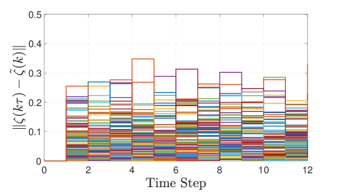
Figure 3. Several realizations of the norm of the error between the outputs of $\Sigma$ and of $\widetilde{\Sigma}$, i.e., $\|\zeta(k\tau)-\tilde{\zeta}(k)\|$, for $T_{d}=12$.

7. Discussion

In this paper, we provided a compositional scheme for constructing finite MDPs of continuous-time stochastic control systems. We first defined notions of stochastic storage and simulation functions between original continuous-time stochastic systems and their discrete-time (finite or infinite) abstractions with and without internal signals. We then leveraged dissipativity-type compositional conditions for the compositional quantification of the distance between the interconnection of concrete continuous-time stochastic control systems and their discrete-time (in)finite abstractions. We focused on a particular class of stochastic affine systems and constructed their finite abstractions together with their corresponding stochastic storage functions. We finally illustrated the effectiveness of our proposed results by applying them to a physical case study.

8. Acknowledgment

The authors would like to thank Abolfazl Lavaei for the fruitful discussions and helpful comments.

9. Appendix

Proof.

(Theorem 4.3) We first show that the SSF $V$ in (4.2) satisfies the inequality (3.3) for some $\mathcal{K}_{\infty}$ function $\alpha$. For any $x=[{x_{1};\ldots;x_{N}}]\in X$ and $\hat{x}=[{\hat{x}_{1};\ldots;\hat{x}_{N}}]\in\hat{X}$, one gets:

$$\|h(x)-\hat{h}(\hat{x})\| =\|[h_{11}(x_{1});\ldots;h_{1N}(x_{N})]-[\hat{h}_{11}(\hat{x}_{1});\ldots;\hat{h}_{1N}(\hat{x}_{N})]\|$$

$$\leq\sum_{i=1}^{N}\|h_{1i}(x_{i})-\hat{h}_{1i}(\hat{x}_{i})\|\leavevmode\nobreak\ \leq\sum_{i=1}^{N}\alpha_{i}^{-1}(S_{i}(x_{i},\hat{x}_{i}))\leq\bar{\alpha}(V(x,\hat{x})),$$

with the function $\bar{\alpha}:\mathbb{R}_{\geq 0}\rightarrow\mathbb{R}_{\geq 0}$ defined for all $s\in\mathbb{R}_{\geq 0}$ as

$\bar{\alpha}(s):=\max\left\{\sum_{i=1}^{N}\alpha_{i}^{-1}(s_{i})\,\,\big{|}\,s_{i}{\geq 0},\,\,\sum_{i=1}^{N}\mu_{i}s_{i}=s\right\}\!.$

By taking the $\mathcal{K}_{\infty}$ function $\alpha(s):=\bar{\alpha}^{-1}(s)$, $\forall s\in{\mathbb{R}}_{\geq 0}$, one acquires

$$\alpha(\|h(x)-\hat{h}(\hat{x})\|)\leq V(x,\hat{x}),$$

fulfilling the inequality (3.3).

We continue with showing (3.4), as well. One can obtain the chain of inequalities in (9.1) using conditions (4.3) and (4.4) and by defining $\kappa(\cdot),\psi,\rho_{\mathrm{ext}}(\cdot)$ as

$$\kappa s :=\max\Big{\{}\sum_{i=1}^{N}\mu_{i}\kappa_{i}s_{i}\,\,\big{|}\,s_{i}{\geq 0},\,\,\sum_{i=1}^{N}\mu_{i}s_{i}=s\Big{\}},$$

$$\rho_{\mathrm{ext}}(s) :=\max\Big{\{}\sum_{i=1}^{N}\mu_{i}\rho_{\mathrm{ext}i}(s_{i})\,\,\big{|}\,s_{i}{\geq 0},\,\,\|{\left[s_{1};\ldots;s_{N}\right]}\|=s\Big{\}},$$

$$\psi :=\sum_{i=1}^{N}\mu_{i}\psi_{i}.$$

Hence one can conclude that $V$ is an SSF from $\widehat{\Sigma}$ to $\Sigma$.

 

$$\mathds{E} \Big{[}V(\xi((k+1)\tau),\hat{\xi}(k+1))\,\big{|}\,\xi,\hat{\xi},\nu,\hat{\nu}\Big{]}=\mathbb{E}\Big{[}\sum_{i=1}^{N}\mu_{i}S_{i}(\xi_{i}((k+1)\tau),\hat{\xi}_{i}(k+1))\,\big{|}\,\xi,\hat{\xi},\nu,\hat{\nu}\Big{]}$$

$$=\sum_{i=1}^{N}\mu_{i}\mathbb{E}\Big{[}S_{i}(\xi_{i}((k+1)\tau),\hat{\xi}_{i}(k+1))\,\big{|}\,\xi,\hat{\xi},\nu,\hat{\nu}\Big{]}=\sum_{i=1}^{N}\mu_{i}\mathbb{E}\Big{[}S_{i}(\xi_{i}((k+1)\tau),\hat{\xi}_{i}(k+1))\,\big{|}\,\xi_{i},\hat{\xi_{i}},\nu_{i},\hat{\nu}_{i}\Big{]}$$

$$\leq\sum_{i=1}^{N}\mu_{i}\bigg{(}\kappa_{i}S_{i}(x_{i},\hat{x}_{i})+\rho_{\mathrm{ext}i}(\|\hat{\nu}_{i}\|)+\psi_{i}+\begin{bmatrix}w_{i}-\hat{w}_{i}\\ h_{2i}(x_{i})-\hat{h}_{2i}(\hat{x}_{i})\end{bmatrix}^{T}\begin{bmatrix}\bar{X}_{i}^{11}&\bar{X}_{i}^{12}\\ \bar{X}_{i}^{21}&\bar{X}_{i}^{22}\end{bmatrix}\begin{bmatrix}w_{i}-\hat{w}_{i}\\ h_{2i}(x_{i})-\hat{h}_{2i}(\hat{x}_{i})\end{bmatrix}\bigg{)}$$

$$=\sum_{i=1}^{N}\mu_{i}\kappa_{i}S_{i}(x_{i},\hat{x}_{i})+\sum_{i=1}^{N}\mu_{i}\rho_{\mathrm{ext}i}(\|\hat{\nu}_{i}\|)+\sum_{i=1}^{N}\mu_{i}\psi_{i}$$

$$\quad+\begin{bmatrix}w_{1}-\hat{w}_{1}\\ \vdots\\ w_{N}-\hat{w}_{N}\\ h_{21}(x_{1})-\hat{h}_{21}(\hat{x}_{1})\\ \vdots\\ h_{2N}(x_{N})-\hat{h}_{2N}(\hat{x}_{N})\end{bmatrix}^{T}\begin{bmatrix}\mu_{1}\bar{X}_{1}^{11}&&&\mu_{1}\bar{X}_{1}^{12}&&\\ &\ddots&&&\ddots&\\ &&\mu_{N}\bar{X}_{N}^{11}&&&\mu_{N}\bar{X}_{N}^{12}\\ \mu_{1}\bar{X}_{1}^{21}&&&\mu_{1}\bar{X}_{1}^{22}&&\\ &\ddots&&&\ddots&\\ &&\mu_{N}\bar{X}_{N}^{21}&&&\mu_{N}\bar{X}_{N}^{22}\end{bmatrix}\begin{bmatrix}w_{1}-\hat{w}_{1}\\ \vdots\\ w_{N}-\hat{w}_{N}\\ h_{21}(x_{1})-\hat{h}_{21}(\hat{x}_{1})\\ \vdots\\ h_{2N}(x_{N})-\hat{h}_{2N}(\hat{x}_{N})\end{bmatrix}$$

$$=\sum_{i=1}^{N}\mu_{i}\kappa_{i}S_{i}(x_{i},\hat{x}_{i})+\sum_{i=1}^{N}\mu_{i}\rho_{\mathrm{ext}i}(\|\hat{\nu}_{i}\|)+\sum_{i=1}^{N}\mu_{i}\psi_{i}$$

$$\quad+\begin{bmatrix}M\begin{bmatrix}h_{21}(x_{1})\\ \vdots\\ h_{2N}(x_{N})\end{bmatrix}-\hat{M}\begin{bmatrix}\hat{h}_{21}(\hat{x}_{1})\\ \vdots\\ \hat{h}_{2N}(\hat{x}_{N})\end{bmatrix}\\ h_{21}(x_{1})-\hat{h}_{21}(\hat{x}_{1})\\ \vdots\\ h_{2N}(x_{N})-\hat{h}_{2N}(\hat{x}_{N})\end{bmatrix}^{T}\!\bar{X}_{cmp}\begin{bmatrix}M\begin{bmatrix}h_{21}(x_{1})\\ \vdots\\ h_{2N}(x_{N})\end{bmatrix}-\hat{M}\begin{bmatrix}\hat{h}_{21}(\hat{x}_{1})\\ \vdots\\ \hat{h}_{2N}(\hat{x}_{N})\end{bmatrix}\\ h_{21}(x_{1})-\hat{h}_{21}(\hat{x}_{1})\\ \vdots\\ h_{2N}(x_{N})-\hat{h}_{2N}(\hat{x}_{N})\end{bmatrix}$$

$$=\sum_{i=1}^{N}\mu_{i}\kappa_{i}S_{i}(x_{i},\hat{x}_{i})+\sum_{i=1}^{N}\mu_{i}\rho_{\mathrm{ext}i}(\|\hat{\nu}_{i}\|)+\sum_{i=1}^{N}\mu_{i}\psi_{i}$$

$$\quad+\begin{bmatrix}h_{21}(x_{1})-\hat{h}_{21}(\hat{x}_{1})\\ \vdots\\ h_{2N}(x_{N})-\hat{h}_{2N}(\hat{x}_{N})\end{bmatrix}^{T}\begin{bmatrix}M\\ \mathds{I}_{\tilde{q}}\end{bmatrix}^{T}\!\bar{X}_{cmp}\begin{bmatrix}M\\ \mathds{I}_{\tilde{q}}\end{bmatrix}\begin{bmatrix}h_{21}(x_{1})-\hat{h}_{21}(\hat{x}_{1})\\ \vdots\\ h_{2N}(x_{N})-\hat{h}_{2N}(\hat{x}_{N})\end{bmatrix}$$

$$\leq\sum_{i=1}^{N}\mu_{i}\kappa_{i}S_{i}(x_{i},\hat{x}_{i})+\sum_{i=1}^{N}\mu_{i}\rho_{\mathrm{ext}i}(\|\hat{\nu}_{i}\|)+\sum_{i=1}^{N}\mu_{i}\psi_{i}\leq\kappa V\left(x,\hat{x}\right)+\rho_{\mathrm{ext}}(\left\|\hat{\nu}\right\|)+\psi.$$ (9.1)

 

∎

Proof.

(Theorem 5.5) Since $\hat{C}_{1}=C_{1}P$, we have $\|C_{1}x-\hat{C}_{1}\hat{x}\|^{2}=(x-P\hat{x})^{T}C_{1}^{T}C_{1}(x-P\hat{x})$. Since $\lambda_{\min}(C_{1}^{T}C_{1})\|x-P\hat{x}\|^{2}\leq(x-P\hat{x})^{T}C_{1}^{T}C_{1}(x-P\hat{x})\leq\lambda_{\max}(C_{1}^{T}C_{1})\|x-P\hat{x}\|^{2}$, and similarly $\lambda_{\min}(\mathcal{\bar{M}})\|x-P\hat{x}\|^{2}\leq(x-P\hat{x})^{T}\mathcal{\bar{M}}(x-P\hat{x})\leq\lambda_{\max}(\mathcal{\bar{M}})\|x-P\hat{x}\|^{2}$, it can be readily verified that $\frac{\lambda_{\min}(\mathcal{\bar{M}})}{\lambda_{\max}(C_{1}^{T}C_{1})}\|C_{1}x-\hat{C}_{1}\hat{x}\|^{2}\leq S(x,\hat{x})$ holds $\forall x\in X$, $\forall\hat{x}\in\hat{X}$, implying that the inequality (3.1) holds with $\alpha(s)=\frac{\lambda_{\min}(\mathcal{\bar{M}})}{\lambda_{\max}(C_{1}^{T}C_{1})}s^{2}$, $\forall s\in{\mathbb{R}}_{\geq 0}$.

We proceed with showing that the inequality (3.2) holds, as well. Using Assumption 5.1, we have

$$\mathds{E} \Big{[}S(\xi((k+1)\tau),\hat{\xi}(k+1))\,\big{|}\,\xi=\xi(k\tau),\hat{\xi}=\hat{\xi}(k),\nu=\nu(k\tau),\hat{\nu}=\hat{\nu}(k),w=w(k\tau),\hat{w}=\hat{w}(k)\Big{]}$$

$$=\mathds{E}\Big{[}S(\xi((k+1)\tau),\hat{\xi}(k+1))\,\big{|}\,\xi,\hat{\xi},\nu,\hat{\nu},w,\hat{w}\Big{]}-\mathds{E}\Big{[}S(\xi((k+1)\tau),\hat{\xi})\big{|}\xi,\hat{\xi},\nu,\hat{\nu},w,\hat{w}\Big{]}$$

$$\quad+\mathds{E}\Big{[}S(\xi((k+1)\tau),\hat{\xi})\,\big{|}\,\xi,\hat{\xi},\nu,\hat{\nu},w,\hat{w}\Big{]}$$

$$\leq\mathds{E}\Big{[}S(\xi((k+1)\tau),\hat{\xi})\,\big{|}\,\xi,\hat{\xi},\nu,\hat{\nu},w,\hat{w}\Big{]}+\mathds{E}\Big{[}\gamma(\|\hat{\xi}(k+1)-\hat{\xi}\|)\,\big{|}\,\hat{\xi},\hat{\nu},\hat{w}\Big{]}.$$

Now by employing Dynkin’s formula [Dyn65], one obtains

$$\mathds{E} \Big{[}S(\xi((k+1)\tau),\hat{\xi})\,\big{|}\,\xi,\hat{\xi},\nu,\hat{\nu},w,\hat{w}\Big{]}+\mathds{E}\Big{[}\gamma(\|\hat{\xi}(k+1)-\hat{\xi}\|)\,\big{|}\,\hat{\xi},\hat{\nu},\hat{w}\Big{]}$$

$$=\mathds{E}_{\varsigma}\Big{[}S(\xi,\hat{\xi})+\mathds{E}\Big{[}\int_{k\tau}^{(k+1)\tau}\!\mathcal{L}S(\xi(t),\hat{\xi})\mathsf{d}t\Big{]}\big{|}\hat{\xi},\hat{\nu},\hat{w}\Big{]}+\mathds{E}\Big{[}\gamma(\|\hat{\xi}(k+1)-\hat{\xi}\|)\big{|}\hat{\xi},\hat{\nu},\hat{w}\Big{]}.$$

Since the infinitesimal generator $\mathcal{L}S$, acting on the function $S$, is defined as

$$\mathcal{L}S(\xi,\hat{\xi})=\partial_{\xi}S(\xi,\hat{\xi})f(\xi,\nu,w)+\frac{1}{2}\text{Tr}(\sigma(\xi)\sigma(\xi)^{T}\partial_{\xi,\xi}S(\xi,\hat{\xi})),$$ (9.2)

where

$$\partial_{\xi}S(\xi,\hat{\xi})=2(\xi(t)-P\hat{\xi})^{T}\mathcal{\bar{M}},\quad\partial_{\xi,\xi}S(\xi,\hat{\xi})=2\mathcal{\bar{M}},$$

one has

$$\mathds{E}_{\varsigma} \Big{[}S(\xi,\hat{\xi})+\mathds{E}\Big{[}\int_{k\tau}^{(k+1)\tau}\!\mathcal{L}S(\xi(t),\hat{\xi})\mathsf{d}t\Big{]}\,\big{|}\,\hat{\xi},\hat{\nu},\hat{w}\Big{]}+\mathds{E}\Big{[}\gamma(\|\hat{\xi}(k+1)-\hat{\xi}\|)\big{|}\hat{\xi},\hat{\nu},\hat{w}\Big{]}$$

$$=\mathds{E}_{\varsigma}\Big{[}S(\xi,\hat{\xi})+\mathds{E}\Big{[}\int_{k\tau}^{(k+1)\tau}\!(2(\xi(t)-P\hat{\xi})^{T}\mathcal{\bar{M}}(A\xi(t)+B\nu(t)+Dw(t)+\mathbf{b})$$

$$\quad+G^{T}\mathcal{\bar{M}}G)\mathsf{d}t\Big{]}\,\big{|}\,\hat{\xi},\hat{\nu},\hat{w}\Big{]}+\mathds{E}\Big{[}\gamma\,(\|\,\hat{\xi}(k+1)-\hat{\xi}\,\|)\,\big{|}\hat{\xi},\hat{\nu},\hat{w}\Big{]}.$$

Given any $\xi(t)$, $\hat{\xi}(k)$, $w(t)$ and $\hat{w}(k)$, we choose $\nu(t)$ via the following interface function:

$$\nu(t) =K(\xi(t)-P\hat{\xi}(k))-Q\hat{\xi}(k)+(\xi(k\tau)-P\hat{\xi}(k))+H(w(k\tau)-\hat{w}(k))-Hw(t),$$ (9.3)

where $k\tau\leq t\leq(k+1)\tau$. By employing conditions (5.2), and (5.2), and the definition of the interface function in (9.3), we have

$$\mathds{E}_{\varsigma} \Big{[}S(\xi,\hat{\xi})+\mathds{E}\Big{[}\int_{k\tau}^{(k+1)\tau}\!(2(\xi(t)-P\hat{\xi})^{T}\mathcal{\bar{M}}(A\xi(t)+B\nu(t)+Dw(t)+\mathbf{b})+G^{T}\mathcal{\bar{M}}G)\mathsf{d}t\Big{]}\,\big{|}\,\hat{\xi},\hat{\nu},\hat{w}\Big{]}$$

$$\quad+\mathds{E}\Big{[}\gamma(\|\hat{\xi}(k+1)-\hat{\xi}\|)\,\big{|}\hat{\xi},\hat{\nu},\hat{w}\Big{]}$$

$$=\mathds{E}_{\varsigma}\Big{[}S(\xi,\hat{\xi})+\mathds{E}\Big{[}\int_{k\tau}^{(k+1)\tau}\!(2\,(\xi(t)-P\hat{\xi})^{T}\mathcal{\bar{M}}((A+BK)(\xi(t)-P\hat{\xi})+B(\xi(k\tau)-P\hat{\xi}(k))+D(w-\hat{w})+\mathbf{b})$$

$$\quad+G^{T}\mathcal{\bar{M}}G)\mathsf{d}t\Big{]}\big{|}\,\hat{\xi},\hat{\nu},\hat{w}\Big{]}+\mathds{E}\Big{[}\gamma(\|\hat{\xi}(k+1)-\hat{\xi}\|)\big{|}\hat{\xi},\hat{\nu},\hat{w}\Big{]}.$$

Using Young’s inequality [You12] as $ab\leq\frac{\pi}{2}a^{2}+\frac{1}{2\pi}b^{2},$ for any $a,b\geq 0$ and any $\pi>0$, by employing Cauchy-Schwarz inequality and using the condition (5.2), one has

$$\mathds{E}_{\varsigma} \Big{[}S(\xi,\hat{\xi})+\mathds{E}\Big{[}\int_{k\tau}^{(k+1)\tau}\!(2\,(\xi(t)-P\hat{\xi})^{T}\mathcal{\bar{M}}((A+BK)(\xi(t)-P\hat{\xi})+B(\xi(k\tau)-P\hat{\xi}(k))+D(w-\hat{w})+\mathbf{b})$$

$$\quad+G^{T}\mathcal{\bar{M}}G)\mathsf{d}t\Big{]}\big{|}\,\hat{\xi},\hat{\nu},\hat{w}\Big{]}+\mathds{E}\Big{[}\gamma(\|\hat{\xi}(k+1)-\hat{\xi}\|)\big{|}\hat{\xi},\hat{\nu},\hat{w}\Big{]}$$

$$\leq\mathds{E}_{\varsigma}\Big{[}S(\xi,\hat{\xi})+\mathds{E}\Big{[}\int_{k\tau}^{(k+1)\tau}\!(-\tilde{\kappa}S(\xi(t),\hat{\xi})+\pi\|\sqrt{\mathcal{\bar{M}}}\mathbf{b}\|^{2}+\pi\|\sqrt{\mathcal{\bar{M}}}B(\xi(k\tau)-P\hat{\xi}(k))\|^{2}+\pi\|\sqrt{\mathcal{\bar{M}}}D(w-\hat{w})\|^{2}$$

$$\quad+G^{T}\mathcal{\bar{M}}G)\mathsf{d}t\Big{]}\big{|}\,\hat{\xi},\hat{\nu},\hat{w}\Big{]}+\mathds{E}\Big{[}\gamma(\|\hat{\xi}(k+1)-\hat{\xi}\|)\,\big{|}\,\hat{\xi},\hat{\nu},\hat{w}\Big{]}$$

$$=\mathds{E}_{\varsigma}\Big{[}S(\xi,\hat{\xi})+\mathds{E}\Big{[}\int_{k\tau}^{(k+1)\tau}\!\!\!-\tilde{\kappa}S(\xi(t),\hat{\xi})\,\mathsf{d}t+\tau(\pi\|\sqrt{\mathcal{\bar{M}}}\mathbf{b}\|^{2}+\pi\|\sqrt{\mathcal{\bar{M}}}B(\xi(k\tau)\!-\!P\hat{\xi}(k))\|^{2}+\pi\|\sqrt{\mathcal{\bar{M}}}D(w-\hat{w})\|^{2}$$

$$\quad+G^{T}\mathcal{\bar{M}}G)\Big{]}\big{|}\,\hat{\xi},\hat{\nu},\hat{w}\Big{]}+\mathds{E}\Big{[}\gamma(\|\hat{\xi}(k+1)-\hat{\xi}\|)\big{|}\hat{\xi},\hat{\nu},\hat{w}\Big{]}.$$

Using Gronwall inequality [Gro19], one has

$$\mathds{E}_{\varsigma} \Big{[}S(\xi,\hat{\xi})+\mathds{E}\Big{[}\int_{k\tau}^{(k+1)\tau}\!-\tilde{\kappa}S(\xi(t),\hat{\xi})\mathsf{d}t+\tau(\pi\|\sqrt{\mathcal{\bar{M}}}\mathbf{b}\|^{2}+\pi\|\sqrt{\mathcal{\bar{M}}}B(\xi(k\tau)-P\hat{\xi}(k))\|^{2}+\pi\|\sqrt{\mathcal{\bar{M}}}D(w-\hat{w})\|^{2}$$

$$\quad+G^{T}\mathcal{\bar{M}}G)\Big{]}\big{|}\,\hat{\xi},\hat{\nu},\hat{w}\Big{]}+\mathds{E}\Big{[}\gamma(\|\hat{\xi}(k+1)-\hat{\xi}\|)\big{|}\hat{\xi},\hat{\nu},\hat{w}\Big{]}$$

$$\leq\mathds{E}_{\varsigma}\Big{[}e^{-\tilde{\kappa}\tau}S(\xi,\hat{\xi})+\mathds{E}\Big{[}e^{-\tilde{\kappa}\tau}\tau(\pi\|\sqrt{\tilde{M}}\mathbf{b}\|^{2}+\pi\|\sqrt{\mathcal{\bar{M}}}B(\xi(k\tau)-P\hat{\xi}(k))\|^{2}+\pi\|\sqrt{\mathcal{\bar{M}}}D(w-\hat{w})\|^{2}$$

$$\quad+G^{T}\mathcal{\bar{M}}G)\Big{]}\big{|}\,\hat{\xi},\hat{\nu},\hat{w}\Big{]}+\mathds{E}\Big{[}\gamma(\|\hat{\xi}(k+1)-\hat{\xi}\|)\,\big{|}\hat{\xi},\hat{\nu},\hat{w}\Big{]}$$

$$=e^{-\tilde{\kappa}\tau}S(\xi,\hat{\xi})+e^{-\tilde{\kappa}\tau}\tau(G^{T}\mathcal{\bar{M}}G+\pi\|\sqrt{\mathcal{\bar{M}}}\mathbf{b}\|^{2}+\pi\|\sqrt{\mathcal{\bar{M}}}B(\xi(k\tau)-P\hat{\xi}(k))\|^{2}+\pi\|\sqrt{\mathcal{\bar{M}}}D(w-\hat{w})\|^{2})$$

$$\quad+\mathds{E}\Big{[}\gamma(\|\hat{\xi}(k+1)-\hat{\xi}\|)\big{|}\hat{\xi},\hat{\nu},\hat{w}\Big{]}$$

$$=e^{-\tilde{\kappa}\tau}S(\xi,\hat{\xi})+e^{-\tilde{\kappa}\tau}\tau(G^{T}\mathcal{\bar{M}}G+\pi\|\sqrt{\mathcal{\bar{M}}}\mathbf{b}\|^{2})+\mathds{E}\Big{[}\gamma(\|\hat{\xi}(k+1)-\hat{\xi}\|)\big{|}\hat{\xi},\hat{\nu},\hat{w}\Big{]}$$

$$\quad+\begin{bmatrix}\xi-P\hat{\xi}\\ w-\hat{w}\\ \end{bmatrix}^{T}\begin{bmatrix}\pi e^{-\tilde{\kappa}\tau}\tau B^{T}\mathcal{\bar{M}}B&&0\\ 0&&\pi e^{-\tilde{\kappa}\tau}\tau D^{T}\mathcal{\bar{M}}D\\ \end{bmatrix}\begin{bmatrix}\xi-P\hat{\xi}\\ w-\hat{w}\\ \end{bmatrix}\!.$$

Employing (5.16) and since $\hat{C}_{2}=C_{2}P$, we have

$$e^{-\tilde{\kappa}\tau}S(\xi,\hat{\xi})+e^{-\tilde{\kappa}\tau}\tau(G^{T}\mathcal{\bar{M}}G+\pi\|\sqrt{\mathcal{\bar{M}}}\mathbf{b}\|^{2})+\mathds{E}\Big{[}\gamma(\|\hat{\xi}(k+1)-\hat{\xi}\|)\big{|}\hat{\xi},\hat{\nu},\hat{w}\Big{]}$$

$$\quad+\begin{bmatrix}\xi-P\hat{\xi}\\ w-\hat{w}\\ \end{bmatrix}^{T}\begin{bmatrix}\pi e^{-\tilde{\kappa}\tau}\tau B^{T}\mathcal{\bar{M}}B&&0\\ 0&&\pi e^{-\tilde{\kappa}\tau}\tau D^{T}\mathcal{\bar{M}}D\\ \end{bmatrix}\begin{bmatrix}\xi-P\hat{\xi}\\ w-\hat{w}\\ \end{bmatrix}$$

$$\leq e^{-\tilde{\kappa}\tau}S(\xi,\hat{\xi})+e^{-\tilde{\kappa}\tau}\tau(G^{T}\mathcal{\bar{M}}G+\pi\|\sqrt{\mathcal{\bar{M}}}\mathbf{b}\|^{2})+\mathds{E}\Big{[}\gamma(\|\hat{\xi}(k+1)-\hat{\xi}\|)\big{|}\hat{\xi},\hat{\nu},\hat{w}\Big{]}$$

$$\quad+\begin{bmatrix}\xi-P\hat{\xi}\\ w-\hat{w}\\ \end{bmatrix}^{T}\begin{bmatrix}\bar{\kappa}\mathcal{\bar{M}}+C_{2}^{T}\bar{X}^{22}C_{2}&C_{2}^{T}\bar{X}^{21}\\ \bar{X}^{12}C_{2}&\bar{X}^{11}\\ \end{bmatrix}\begin{bmatrix}\xi-P\hat{\xi}\\ w-\hat{w}\\ \end{bmatrix}$$

$$=(\bar{\kappa}+e^{-\tilde{\kappa}\tau})S(\xi,\hat{\xi})+e^{-\tilde{\kappa}\tau}\tau(G^{T}\mathcal{\bar{M}}G+\pi\|\sqrt{\mathcal{\bar{M}}}\mathbf{b}\|^{2})+\mathds{E}\Big{[}\gamma(\|\hat{\xi}(k+1)-\hat{\xi}\|)\big{|}\hat{\xi},\hat{\nu},\hat{w}\Big{]}$$

$$\quad+\begin{bmatrix}w-\hat{w}\\ C_{2}\xi-\hat{C}_{2}\hat{\xi}\\ \end{bmatrix}^{T}\begin{bmatrix}\bar{X}^{11}&\bar{X}^{12}\\ \bar{X}^{21}&\bar{X}^{22}\\ \end{bmatrix}\begin{bmatrix}w-\hat{w}\\ C_{2}\xi-\hat{C}_{2}\hat{\xi}\\ \end{bmatrix}\!.$$

Since the function $\gamma$ defined in Assumption 5.1 is concave, using Jensen inequality one has

$$\mathds{E} \Big{[}\gamma(\|\hat{\xi}(k+1)-\hat{\xi}\|)\,\big{|}\,\hat{\xi},\hat{\nu},\hat{w}\Big{]}=\mathds{E}\Big{[}\gamma(\|\hat{\xi}(k+1)-(\hat{\xi}+\hat{\nu}+\tilde{D}\,\hat{w}+\tilde{R}\varsigma)+(\hat{\xi}+\hat{\nu}+\tilde{D}\,\hat{w}+\tilde{R}\varsigma)-\hat{\xi}\|)\,\big{|}\,\hat{\xi},\hat{\nu},\hat{w}\Big{]}$$

$$\leq\mathds{E}\Big{[}\gamma(\delta+\|\hat{\nu}+\tilde{D}\hat{w}+\tilde{R}\varsigma\|)\,\big{|}\,\hat{\xi},\hat{\nu},\hat{w}\Big{]}$$

$$\leq\gamma((1+\bar{\eta})\delta)+\mathds{E}\Big{[}\gamma((1+\frac{1}{\bar{\eta}})\|\hat{\nu}+\tilde{D}\hat{w}+\tilde{R}\varsigma\|)\,\big{|}\,\hat{\xi},\hat{\nu},\hat{w}\Big{]}$$

$$\leq\gamma((1+\bar{\eta})\delta)+\gamma((1+\frac{1}{\bar{\eta}})(1+\bar{\eta}^{\prime})\|\hat{\nu}+\tilde{D}\,\hat{w}\|)+\gamma((1+\frac{1}{\bar{\eta}})(1+\frac{1}{\bar{\eta}^{\prime}})\mathds{E}\Big{[}\|\tilde{R}\varsigma\|\,\big{|}\,\hat{\xi},\hat{\nu},\hat{w}\Big{]})$$

$$=\gamma((1+\bar{\eta})\delta)+\gamma((1+\frac{1}{\bar{\eta}})(1+\bar{\eta}^{\prime})\|\hat{\nu}+\tilde{D}\,\hat{w}\|)+\gamma((1+\frac{1}{\bar{\eta}})(1+\frac{1}{\bar{\eta}^{\prime}})\mathds{E}\Big{[}([\tilde{R}\varsigma]^{T}[\tilde{R}\varsigma])^{\tfrac{1}{2}}\big{|}\,\hat{\xi},\hat{\nu},\hat{w}\Big{]})$$

$$\leq\gamma((1+\bar{\eta})\delta)+\gamma((1+\frac{1}{\bar{\eta}})(1+\bar{\eta}^{\prime})(1+\bar{\eta}^{\prime\prime})\|\hat{\nu}\|)+\gamma((1+\frac{1}{\bar{\eta}})(1+\bar{\eta}^{\prime})(1+\frac{1}{\bar{\eta}^{\prime\prime}})\|\tilde{D}\,\|\,\|\hat{w}\|)$$

$$\quad+\gamma((1+\frac{1}{\bar{\eta}})(1+\frac{1}{\bar{\eta}^{\prime}})(\mathds{E}\Big{[}[\tilde{R}\varsigma]^{T}[\tilde{R}\varsigma]\,\big{|}\,\hat{\xi},\hat{\nu},\hat{w}\Big{]})^{\tfrac{1}{2}})$$

$$=\gamma((1+\bar{\eta})\delta)+\gamma((1+\frac{1}{\bar{\eta}})(1+\bar{\eta}^{\prime})(1+\bar{\eta}^{\prime\prime})\|\hat{\nu}\|)+\gamma((1+\frac{1}{\bar{\eta}})(1+\bar{\eta}^{\prime})(1+\frac{1}{\bar{\eta}^{\prime\prime}})\,\|\tilde{D}\,\|\,\|\hat{w}\|)$$

$$\quad+\gamma((1+\frac{1}{\bar{\eta}})(1+\frac{1}{\bar{\eta}^{\prime}})\sqrt{\text{Tr}(\tilde{R}^{T}\tilde{R})}),$$ (9.4)

where $\bar{\eta},\bar{\eta}^{\prime},\bar{\eta}^{\prime\prime}\in\mathbb{R}_{>0}$. Then one can conclude that

$$\mathds{E} \Big{[}S(\xi((k+1)\tau),\hat{\xi}(k+1))\,\big{|}\,\xi,\hat{\xi},\nu,\hat{\nu},w,\hat{w}\Big{]}$$

$$\leq(\bar{\kappa}+e^{-\tilde{\kappa}\tau})S(\xi,\hat{\xi})+\gamma((1+\frac{1}{\bar{\eta}})(1+\bar{\eta}^{\prime})(1+\bar{\eta}^{\prime\prime})\|\hat{\nu}\|)+e^{-\tilde{\kappa}\tau}\tau(G^{T}\mathcal{\bar{M}}G+\pi\|\sqrt{\mathcal{\bar{M}}}\mathbf{b}\|^{2})+\gamma((1+\bar{\eta})\delta)$$

$$\quad+\gamma((1+\frac{1}{\bar{\eta}})(1+\frac{1}{\bar{\eta}^{\prime}})\sqrt{\text{Tr}(\tilde{R}^{T}\tilde{R})})+\gamma((1+\frac{1}{\bar{\eta}})(1+\bar{\eta}^{\prime})(1+\frac{1}{\bar{\eta}^{\prime\prime}})\,\|\tilde{D}\,\|\,\|\hat{w}\|)$$

$$\quad+\begin{bmatrix}w-\hat{w}\\ C_{2}\xi-\hat{C}_{2}\hat{\xi}\\ \end{bmatrix}^{T}\begin{bmatrix}\bar{X}^{11}&\bar{X}^{12}\\ \bar{X}^{21}&\bar{X}^{22}\\ \end{bmatrix}\begin{bmatrix}w-\hat{w}\\ C_{2}\xi-\hat{C}_{2}\hat{\xi}\\ \end{bmatrix}\!,$$ (9.5)

which completes the proof with

$$\alpha(s) :=\frac{\lambda_{\min}(\mathcal{\bar{M}})}{\lambda_{\max}(C_{1}^{T}C_{1})}s^{2},\quad\forall s\in{\mathbb{R}}_{\geq 0},$$

$$\kappa :=\bar{\kappa}+e^{-\tilde{\kappa}\tau},$$

$$\rho_{\mathrm{ext}}(s) :=\gamma((1+\frac{1}{\bar{\eta}})(1+\bar{\eta}^{\prime})(1+\bar{\eta}^{\prime\prime})s),\quad\forall s\in{\mathbb{R}}_{\geq 0},$$

$$\psi :=e^{-\bar{\kappa}\tau}\tau(G^{T}\mathcal{\bar{M}}G+\pi\|\sqrt{\mathcal{\bar{M}}}\mathbf{b}\|^{2})+\gamma((1+\bar{\eta})\delta)+\gamma((1+\frac{1}{\bar{\eta}})(1+\frac{1}{\bar{\eta}^{\prime}})\sqrt{\text{Tr}(\tilde{R}^{T}\tilde{R})})$$

$$\quad+\gamma((1+\frac{1}{\bar{\eta}})(1+\bar{\eta}^{\prime})(1+\frac{1}{\bar{\eta}^{\prime\prime}})\,\|\tilde{D}\,\|\,\|\hat{w}\|).$$

∎

Remark 9.1.

Note that the infinitesimal generator $\mathcal{L}S(x,\hat{x})$ defined in (9.2) is different from the usual one employed in [ZMEM⁺14] since the abstract system $\widehat{\Sigma}$ in this paper is considered in the discrete-time domain.

References

- [AMP16] M. Arcak, C. Meissen, and A. Packard. Networks of dissipative systems. SpringerBriefs in Electrical and Computer Engineering. Springer, 2016.
- [APLS08] A. Abate, M. Prandini, J. Lygeros, and S. Sastry. Probabilistic reachability and safety for controlled discrete-time stochastic hybrid systems. Automatica, 44(11):2724–2734, 2008.
- [Bel65] H. E. Bell. Gershgorin’s theorem and the zeros of polynomials. The American Mathematical Monthly, 72(3):292–295, 1965.
- [BS96] D. P. Bertsekas and S. E. Shreve. Stochastic optimal control: The discrete-time case. Athena Scientific, 1996.
- [CA19] N. Cauchi and A. Abate. StocHy: Automated verification and synthesis of stochastic processes. In Proceedings of the International Conference on Tools and Algorithms for the Construction and Analysis of Systems, pages 247–264. Springer, 2019.
- [Dyn65] E. B. Dynkin. Markov processes. pages 77–104. Springer, 1965.
- [GGM16] A. Girard, G. Gössler, and S. Mouelhi. Safety controller synthesis for incrementally stable switched systems using multiscale symbolic models. IEEE Transactions on Automatic Control, 61(6):1537–1549, 2016.
- [Gro19] T. H. Gronwall. Note on the derivatives with respect to a parameter of the solutions of a system of differential equations. Annals of Mathematics, pages 292–296, 1919.
- [HSA17] Sofie Haesaert, Sadegh Soudjani, and Alessandro Abate. Verification of general Markov decision processes by approximate similarity relations and policy refinement. In SIAM Journal on Control and Optimization, volume 55, pages 2333–2367, 2017.
- [JP09] A. A. Julius and G. J. Pappas. Approximations of stochastic hybrid systems. IEEE Transactions on Automatic Control, 54(6):1193–1203, 2009.
- [Kal97] O. Kallenberg. Foundations of modern probability. Springer-Verlag, New York, 1997.
- [KSL13] Maryam Kamgarpour, Sean Summers, and John Lygeros. Control design for specifications on stochastic hybrid systems. In Proceedings of the 16th International Conference on Hybrid Systems: Computation and Control, HSCC ’13, pages 303–312, New York, NY, USA, 2013. ACM.
- [LAB+17] L. Laurenti, A. Abate, L. Bortolussi, L. Cardelli, M. Ceska, and M. Kwiatkowska. Reachability computation for switching diffusions: Finite abstractions with certifiable and tuneable precision. In Proceedings of the 20th ACM International Conference on Hybrid Systems: Computation and Control, pages 55–64, 2017.
- [Lav19] A. Lavaei. Automated Verification and Control of Large-Scale Stochastic Cyber-Physical Systems: Compositional Techniques. PhD thesis, Technische Universität München, Germany, 2019.
- [LSMZ17] A. Lavaei, S. Soudjani, R. Majumdar, and M. Zamani. Compositional abstractions of interconnected discrete-time stochastic control systems. In Proceedings of the 56th IEEE Conference on Decision and Control, pages 3551–3556, 2017.
- [LSZ18a] A. Lavaei, S. Soudjani, and M. Zamani. Compositional synthesis of finite abstractions for continuous-space stochastic control systems: A small-gain approach. In Proceedings of the 6th IFAC Conference on Analysis and Design of Hybrid Systems, volume 51, pages 265–270, 2018.
- [LSZ18b] A. Lavaei, S. Soudjani, and M. Zamani. From dissipativity theory to compositional construction of finite Markov decision processes. In Proceedings of the 21st ACM International Conference on Hybrid Systems: Computation and Control, pages 21–30, 2018.
- [LSZ19a] A. Lavaei, S. Soudjani, and M. Zamani. Compositional abstraction-based synthesis of general MDPs via approximate probabilistic relations. arXiv: 1906.02930, June 2019.
- [LSZ19b] A. Lavaei, S. Soudjani, and M. Zamani. Compositional construction of infinite abstractions for networks of stochastic control systems. Automatica, 107:125–137, 2019.
- [LSZ19c] A. Lavaei, S. Soudjani, and M. Zamani. Compositional synthesis of not necessarily stabilizable stochastic systems via finite abstractions. In Proceedings of the 18th European Control Conference, pages 2802–2807, 2019.
- [LSZ20a] A. Lavaei, S. Soudjani, and M. Zamani. Compositional abstraction-based synthesis for networks of stochastic switched systems. Automatica, 114, 2020.
- [LSZ20b] A. Lavaei, S. Soudjani, and M. Zamani. Compositional abstraction of large-scale stochastic systems: A relaxed dissipativity approach. Nonlinear Analysis: Hybrid Systems, 36, 2020.
- [LSZ20c] A. Lavaei, S. Soudjani, and M. Zamani. Compositional (in)finite abstractions for large-scale interconnected stochastic systems. IEEE Transactions on Automatic Control, DOI: 10.1109/TAC.2020.2975812, 2020.
- [LZ19] A. Lavaei and M. Zamani. Compositional construction of finite MDPs for large-scale stochastic switched systems: A dissipativity approach. Proceedings of the 15th IFAC Symposium on Large Scale Complex Systems: Theory and Applications, 52(3):31–36, 2019.
- [NSZ19] A. Nejati, S. Soudjani, and M. Zamani. Abstraction-based synthesis of continuous-time stochastic control systems. In Proceedings of the 18th European Control Conference, pages 3212–3217, 2019.
- [NSZ20] A. Nejati, S. Soudjani, and M. Zamani. Compositional abstraction-based synthesis for continuous-time stochastic hybrid systems. European Journal of Control, to appear, 2020.
- [Pnu77] A. Pnueli. The temporal logic of programs. In Proceedings of the 18th IEEE Annual Symposium on Foundations of Computer Science, pages 46–57, 1977.
- [RZ16] M. Rungger and M. Zamani. SCOTS: A tool for the synthesis of symbolic controllers. In Proceedings of the 19th ACM International Conference on Hybrid Systems: Computation and Control, pages 99–104, 2016.
- [SA13] S. Soudjani and A. Abate. Adaptive and sequential gridding procedures for the abstraction and verification of stochastic processes. SIAM Journal on Applied Dynamical Systems, 12(2):921–956, 2013.
- [SAM17] Sadegh Soudjani, Alessandro Abate, and Rupak Majumdar. Dynamic Bayesian networks for formal verification of structured stochastic processes. Acta Informatica, 54(2):217–242, Mar 2017.
- [SGA15] S. Soudjani, C. Gevaerts, and A. Abate. FAUST: Formal abstractions of uncountable-state stochastic processes. In TACAS’15, volume 9035 of Lecture Notes in Computer Science, pages 272–286. Springer, 2015.
- [Sou14] S. Soudjani. Formal Abstractions for Automated Verification and Synthesis of Stochastic Systems. PhD thesis, Technische Universiteit Delft, The Netherlands, 2014.
- [TMKA13] I. Tkachev, A. Mereacre, Joost-Pieter Katoen, and A. Abate. Quantitative automata-based controller synthesis for non-autonomous stochastic hybrid systems. In Proceedings of the 16th ACM International Conference on Hybrid Systems: Computation and Control, pages 293–302, 2013.
- [You12] W. H. Young. On classes of summable functions and their Fourier series. Proceedings of the Royal Society of London A: Mathematical, Physical and Engineering Sciences, 87(594):225–229, 1912.
- [ZA14] M. Zamani and A. Abate. Approximately bisimilar symbolic models for randomly switched stochastic systems. Systems & Control Letters, 69:38–46, 2014.
- [ZAG15] M. Zamani, A. Abate, and A. Girard. Symbolic models for stochastic switched systems: A discretization and a discretization-free approach. Automatica, 55:183–196, 2015.
- [ZMEM+14] M. Zamani, P. Mohajerin Esfahani, R. Majumdar, A. Abate, and J. Lygeros. Symbolic control of stochastic systems via approximately bisimilar finite abstractions. IEEE Transactions on Automatic Control, 59(12):3135–3150, 2014.
- [ZRME17] M. Zamani, M. Rungger, and P. Mohajerin Esfahani. Approximations of stochastic hybrid systems: A compositional approach. IEEE Transactions on Automatic Control, 62(6):2838–2853, 2017.