Unified Formula for Stationary Josephson Current in Planar Graphene Junctions

Abstract

The stationary Josephson current in a ballistic graphene system is theoretically studied with focus on a planar junction consisting of a monolayer graphene sheet on top of which a pair of superconducting electrodes is deposited. To characterize such a planar junction, we employ two parameters: the coupling strength between the graphene sheet and the superconducting electrodes, and a potential drop induced in the graphene sheet by direct contact with the electrodes. We derive a general formula for the Josephson current by taking these parameters into account in addition to other basic parameters, such as temperature and chemical potential. The resulting formula applies to a wide range of parameters and reproduces previously reported results in certain limits.

1 Introduction

For more than a decade, the Josephson effect [1] in a superconductor-graphene-superconductor (SGS) junction has attracted considerable theoretical [2, 3, 4, 5, 6, 7, 8, 9, 10, 11, 12, 13, 14] and experimental [15, 16, 17, 18, 19, 20, 21, 22, 23, 24, 25, 26, 27, 28, 29, 30, 31, 32] interest. In most studies, researchers attempted to observe how the stationary Josephson current is affected by the unique band structure of a graphene sheet, [33, 34] in which the conduction and valence bands touch conically at $K_{+}$ and $K_{-}$ points in the Brillouin zone (the Dirac points). In early experiments, such an attempt was not easy to succeed because the graphene sheet used to fabricate an SGS junction is not sufficiently clean, thus, electron motion cannot be ballistic in it. However, the encapsulation technique of a graphene sheet enables us to fabricate a nearly ideal SGS junction [15, 27, 28, 26, 29, 30, 31, 32] in which the electron motion is ballistic. In such an SGS junction, the unique band structure of a graphene sheet should manifest itself in various features of the Josephson current. To elucidate such features, a general theoretical description of the Josephson current is highly desirable.

Here, we briefly review a theoretical study by Titov and Beenakker, [3] which serves as a starting point of the theoretical approach to the Josephson effect in an SGS junction. The SGS junction considered in Ref. titov is depicted in Fig. 1, where two superconductors $\rm S_{1}$ ($L/2\leq x$) and $\rm S_{2}$ ($x\leq-L/2$) of width $W$ are placed with separation $L$ on top of a clean monolayer graphene sheet with the condition of $L\ll W$. In Ref. titov, it is assumed that electron states in the graphene sheet are described by a massless Dirac equation, and that the carrier doping in the covered region of $L/2\leq|x|$ is described by an effective potential of a negative constant $-U$. [35] In Ref. titov, it is also assumed that the superconducting proximity effect on the graphene sheet is described by an energy-independent effective pair potential $\Delta_{\rm eff}$, which is constant in the covered region ($L/2\leq|x|$) and vanishes in the uncovered region ($|x|\leq L/2$). The important parameters characterizing the Josephson current in this model are $L$, $U$, and $\Delta_{\rm eff}$, in addition to temperature $T$ and chemical potential $\mu$. By taking the limit of $U\to\infty$, the authors of Ref. titov derived a formula for the Josephson current at $T=0$ in the short junction limit of $L\ll\xi$, where $\xi$ is the superconducting coherence length. The formula, given in Eq. (19) of Ref. titov, applies to $0\leq\mu$ [36] under the condition of $T=0$, $L\ll\xi$, and $U\to\infty$.

The assumption of $\Delta_{\rm eff}$ being energy-independent was examined in Refs. takane1 and takane2 to improve the description of the superconducting proximity effect. In Refs. takane1 and takane2, the proximity effect is described by treating the coupling between the graphene sheet and the superconducting electrodes in terms of a tunneling Hamiltonian. [37, 38] Instead of using $\Delta_{\rm eff}$, this approach adopts a parameter $\Gamma$ that controls the strength of the tunnel coupling, enabling us to take into account the energy dependence of the effective pair potential. It is shown that the resulting formula, given in Eq. (53) of Ref. takane2, cohesively describes various behaviors of the Josephson critical current $I_{c}$ as a function of $T$ observed in a set of samples. [30] In particular, it succeeds in describing the unusual $T$ dependence of $I_{c}$ in an SGS junction with a relatively weak coupling. A drawback of this formula is that its application is restricted to the case of $\mu$ being sufficiently away from the Dirac point. This is ascribed to a quasiclassical approximation used in its derivation.

The purpose of this study is to give a general formula for the stationary Josephson current through a monolayer graphene sheet, which can be applied to a wide range of parameters. To do so, we adopt the model used in Ref. takane2 and derive a general formula for the Josephson current without relying on a quasiclassical approximation. The resulting formula applies to arbitrary $T$, $\mu$, $L$, $U$, and $\Gamma$, [39] and reproduces the formulas of Refs. titov and takane2 in certain limits. The paper is organized as follows. In Sect. 2, we describe the model for the SGS junction and introduce a thermal Green’s function. In Sect. 3, we construct the thermal Green’s function and then derive a general formula for the Josephson current. In Sect. 4, we show that the resulting formula reproduces the results of Refs. titov and takane2 in certain limits. In Sect. 5, the behavior of the Josephson critical current is numerically studied in a short junction limit. Section 6 is devoted to a summary. We set $k_{\rm B}=\hbar=1$ throughout the paper.

2 Model and Thermal Green’s Function

We consider an SGS junction of monolayer graphene as depicted in Fig. 1. We adopt a model described in Ref. takane2 and then introduce a thermal Green’s function that is convenient for the subsequent analysis of the Josephson current,

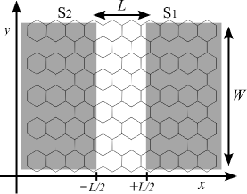
Figure 1: Josephson junction consisting of a monolayer graphene sheet on which two superconductors ${\rm S}_{1}$ and ${\rm S}_{2}$ of width $W$ are deposited with separation $L$.

In Fig. 1, two superconductors ${\rm S}_{1}$ and ${\rm S}_{2}$ of width $W$ are placed with separation $L$ on top of a clean monolayer graphene sheet, where ${\rm S}_{1}$ and ${\rm S}_{2}$ respectively occupy the regions of $L/2\leq x$ and of $x\leq-L/2$. We assume that the pair potential is given by

$$\Delta(x)=\left\{\begin{array}[]{cc}\Delta e^{i\varphi/2}&(L/2<x)\\ 0&(|x|<L/2)\\ \Delta e^{-i\varphi/2}&(x<-L/2),\end{array}\right.$$ (4)

where $\varphi$ serves as the phase difference between the two superconducting electrodes.

Let us assume that the coupling of the graphene sheet and the superconductors is described by a tunneling Hamiltonian. The resulting proximity effect on the graphene sheet is described by a self-energy [37, 38] [see Eq. (22)]. The coupling with the superconductors also induces carrier doping in the graphene sheet; the carrier density in the covered region of $L/2<|x|$ becomes higher than that in the uncovered region of $|x|<L/2$. We describe this by adding the effective potential of a negative constant $-U$ only in the covered region, [3] resulting in the renormalization of the chemical potential $\mu$:

$$\tilde{\mu}=\left\{\begin{array}[]{cc}\mu&(|x|<L/2)\\ \mu+U&(L/2<|x|).\end{array}\right.$$ (7)

Let us turn to the electron states in the graphene sheet. Low-energy states appear in the two valleys located at the $K_{+}$ and $K_{-}$ points in the Brillouin zone, where the wave vector corresponding to the $K_{\pm}$ point is given by $\mib{K}_{\pm}=\pm(2\pi/a)(2/3,0)$ with $a$ being the lattice constant of the graphene sheet. Within the effective mass approximation, the low-energy states in the $K_{\pm}$ valley are described by the effective Hamiltonian $H_{\pm}$ defined by [40, 41, 42]

$$H_{\pm} =\left(\begin{array}[]{cc}-\tilde{\mu}&\gamma k_{\mp}\\ \gamma k_{\pm}&-\tilde{\mu}\end{array}\right),$$ (10)

where $k_{\pm}=k_{x}\pm ik_{y}$ with $k_{x}=-i\partial_{x}$ and $k_{y}=-i\partial_{y}$. The $2\times 2$ form of $H_{\pm}$ reflects the fact that the unit cell of a hexagonal lattice contains A and B sites, and $\gamma$ is given by $\gamma=(\sqrt{3}/2)\gamma_{0}a$, where $\gamma_{0}$ represents the nearest-neighbor transfer integral. [40, 41, 42]

In the presence of the superconducting proximity effect, we need to treat electron and hole states taking their coupling into account. The simplest way to do this is to employ a Bogoliubov–de Gennes equation:

$$H_{\rm BdG}\left(\begin{array}[]{c}\Psi_{e}\\ \Psi_{h}\end{array}\right)=\epsilon\left(\begin{array}[]{c}\Psi_{e}\\ \Psi_{h}\end{array}\right),$$ (15)

where $\Psi_{e}$ and $\Psi_{h}$ are respectively the electron and hole wavefunctions, and the $4\times 4$ Hamiltonian for the $K_{+}$ valley is given by [43]

$$H_{\rm BdG}=\left(\begin{array}[]{cc}H_{+}&\Delta_{\rm eff}(x)\sigma_{0}\\ \Delta_{\rm eff}(x)^{*}\sigma_{0}&-H_{+}\end{array}\right)$$ (18)

with $\sigma_{0}={\rm diag}(1,1)$. Here, $\Delta_{\rm eff}(x)$ is the effective pair potential, which is usually assumed to be an energy-independent constant in the covered region. This widely accepted assumption for $\Delta_{\rm eff}$ is justified only when the coupling between the graphene sheet and the superconducting electrodes is sufficiently strong. [11, 38] To cope with arbitrary coupling strength, we employ the tunneling Hamiltonian model proposed by McMillan [37] instead of assuming the energy-independent pair potential. The approach of McMillan is reformulated in Ref. takane3 in the form specific to a hybrid graphene system.

We introduce the $4\times 4$ thermal Green’s function $G(\mib{r},\mib{r}^{\prime};\omega)$ with $\omega=(2n+1)\pi T$, which obeys

$$\left(i\omega\tau^{0}-H-\Sigma\right)G(\mib{r},\mib{r}^{\prime};\omega)=\tau^{0}\delta(\mib{r}-\mib{r}^{\prime}),$$ (19)

where $H={\rm diag}(H_{+},-H_{+})$ and $\tau^{0}={\rm diag}(1,1,1,1)$. The self-energy $\Sigma$, representing the proximity effect mediated by quasiparticle tunneling, is given by [10, 38]

$$\Sigma =\frac{-\Gamma\theta\left(|x|-\frac{L}{2}\right)}{\sqrt{\Delta^{2}+\omega^{2}}}\left(\begin{array}[]{cc}i\omega&\Delta(x)\\ \Delta(x)^{*}&i\omega\end{array}\right)\otimes\sigma_{0},$$ (22)

where $\Gamma$ represents the strength of the tunnel coupling and $\theta(x)$ is the Heaviside step function. The off-diagonal elements are regarded as an energy-dependent effective pair potential, while the diagonal elements describe the renormalization of a quasiparticle energy. Here and hereafter, we restrict our consideration to quasiparticle states in the $K_{+}$ valley because those in the $K_{-}$ valley equivalently contribute to the Josephson current. A brief comment on $G(\mib{r},\mib{r}^{\prime};\omega)$ is given in Appendix A.

3 Formulation

We derive a general formula for the Josephson current by using an analytical expression of the thermal Green’s function on the basis of the argument originally given by Ishii [44, 45] and later developed by Furusaki and Tsukada. [46, 47, 48]

Hereafter, we restrict our attention to the regime of electron doping: $0\leq\mu<\mu+U$. Assuming that our system is translationally invariant in the $y$ direction, we perform the Fourier transformation:

$$G(x,x^{\prime};q,\omega)=\int d(y-y^{\prime})e^{-iq(y-y^{\prime})}G(\mib{r},\mib{r}^{\prime};\omega),$$ (23)

which we explicitly express as

$$G(x,x^{\prime};q,\omega)=\left(\begin{array}[]{cc}g(x,x^{\prime};q,\omega)&f^{\prime}(x,x^{\prime};q,\omega)\\ f^{\dagger}(x,x^{\prime};q,\omega)&g^{\prime}(x,x^{\prime};q,\omega)\end{array}\right).$$ (26)

Note that we need to treat only $g(x,x^{\prime};q,\omega)$ and $f^{\dagger}(x,x^{\prime};q,\omega)$. Let us consider them in the uncovered region of $|x|<L/2$. It is convenient to define the wave numbers in the $x$-direction as

$$k_{e} ={\rm sgn}_{\omega}\sqrt{\left(\frac{\mu+i\omega}{\gamma}\right)^{2}-q^{2}},$$ (27)

$$k_{h} ={\rm sgn}_{\omega}\sqrt{\left(\frac{\mu-i\omega}{\gamma}\right)^{2}-q^{2}},$$ (28)

where ${\rm Im}\{k_{e}\}>0$ and ${\rm Im}\{k_{h}\}<0$, and ${\rm sgn}_{\omega}$ represents the sign of $\omega$. It is also convenient to introduce

$$e^{\pm i\phi_{e}}=\frac{\gamma(k_{e}\pm iq)}{\mu+i\omega},$$ (29)

$$e^{\pm i\phi_{h}}=\frac{\gamma(k_{h}\pm iq)}{\mu-i\omega}.$$ (30)

This is equivalent to defining

$$\cos\phi_{e}=\frac{\gamma k_{e}}{\mu+i\omega},\hskip 14.22636pt\sin\phi_{e}=\frac{\gamma q}{\mu+i\omega},$$ (31)

$$\cos\phi_{h}=\frac{\gamma k_{h}}{\mu-i\omega},\hskip 14.22636pt\sin\phi_{h}=\frac{\gamma q}{\mu-i\omega}.$$ (32)

If $\mu$ is sufficiently away from the Dirac point, the Josephson current is carried by propagating modes. References takane1 and takane2 focus on this case, in which $k_{e}$ and $k_{h}$, respectively, can be approximated as Eqs. (87) and (88), reproducing the result of a quasiclassical Green’s function approach. [10, 11] Contrastingly, if $\mu$ is very near the Dirac point, the Josephson current is carried by evanescent modes. In this study, we treat these two different cases as well as an intermediate case in a unified manner.

A general solution of $g(x,x^{\prime};q,\omega)$ is written as

$$g(x,x^{\prime};q,\omega) =\left[-\frac{i}{v_{e}}\theta(x-x^{\prime})+c_{++}\right]e^{ik_{e}(x-x^{\prime})}\Lambda^{++}_{e}$$

$$+\left[-\frac{i}{v_{e}}\theta(x^{\prime}-x)+c_{--}\right]e^{-ik_{e}(x-x^{\prime})}\Lambda^{--}_{e}$$

$$+c_{+-}e^{ik_{e}(x+x^{\prime})}\Lambda^{+-}_{e}+c_{-+}e^{-ik_{e}(x+x^{\prime})}\Lambda^{-+}_{e},$$ (33)

where $v_{e}=\gamma\cos\phi_{e}$ and

$$\Lambda^{++}_{e} =\frac{1}{2}\left(\begin{array}[]{cc}1&e^{-i\phi_{e}}\\ e^{i\phi_{e}}&1\end{array}\right),$$ (36)

$$\Lambda^{--}_{e} =\frac{1}{2}\left(\begin{array}[]{cc}1&-e^{i\phi_{e}}\\ -e^{-i\phi_{e}}&1\end{array}\right),$$ (39)

$$\Lambda^{+-}_{e} =\frac{1}{2}\left(\begin{array}[]{cc}e^{-i\phi_{e}}&-1\\ 1&-e^{i\phi_{e}}\end{array}\right),$$ (42)

$$\Lambda^{-+}_{e} =\frac{1}{2}\left(\begin{array}[]{cc}e^{i\phi_{e}}&1\\ -1&-e^{-i\phi_{e}}\end{array}\right).$$ (45)

A general solution of $f^{\dagger}(x,x^{\prime};q,\omega)$ is written as

$$f^{\dagger}(x,x^{\prime};q,\omega)$$

$$=d_{++}e^{i(k_{h}x-k_{e}x^{\prime})}\Lambda^{++}_{h}+d_{--}e^{-i(k_{h}x-ik_{e}x^{\prime})}\Lambda^{--}_{h}$$

$$+d_{+-}e^{i(k_{h}x+k_{e}x^{\prime})}\Lambda^{+-}_{h}+d_{-+}e^{-i(k_{h}x+k_{e}x^{\prime})}\Lambda^{-+}_{h},$$ (46)

where

$$\Lambda^{++}_{h} =\frac{1}{2}\left(\begin{array}[]{cc}e^{-\frac{i}{2}(\phi_{h}-\phi_{e})}&e^{-\frac{i}{2}(\phi_{h}+\phi_{e})}\\ e^{\frac{i}{2}(\phi_{h}+\phi_{e})}&e^{\frac{i}{2}(\phi_{h}-\phi_{e})}\end{array}\right),$$ (49)

$$\Lambda^{--}_{h} =\frac{1}{2}\left(\begin{array}[]{cc}e^{\frac{i}{2}(\phi_{h}-\phi_{e})}&-e^{\frac{i}{2}(\phi_{h}+\phi_{e})}\\ -e^{-\frac{i}{2}(\phi_{h}+\phi_{e})}&e^{-\frac{i}{2}(\phi_{h}-\phi_{e})}\end{array}\right),$$ (52)

$$\Lambda^{+-}_{h} =\frac{1}{2}\left(\begin{array}[]{cc}e^{-\frac{i}{2}(\phi_{h}+\phi_{e})}&-e^{-\frac{i}{2}(\phi_{h}-\phi_{e})}\\ e^{\frac{i}{2}(\phi_{h}-\phi_{e})}&-e^{\frac{i}{2}(\phi_{h}+\phi_{e})}\end{array}\right),$$ (55)

$$\Lambda^{-+}_{h} =\frac{1}{2}\left(\begin{array}[]{cc}e^{\frac{i}{2}(\phi_{h}+\phi_{e})}&e^{\frac{i}{2}(\phi_{h}-\phi_{e})}\\ -e^{-\frac{i}{2}(\phi_{h}-\phi_{e})}&-e^{-\frac{i}{2}(\phi_{h}+\phi_{e})}\end{array}\right).$$ (58)

The Josephson current is formally expressed as

$$I(\varphi)=4W\int_{-\infty}^{+\infty}\frac{dq}{2\pi}T\sum_{\omega}{\rm tr}\left\{j_{x}g(x;q,\omega)\right\},$$ (59)

where the factor $4$ comes from the spin and valley degeneracies, the current operator $j_{x}$ is defined by

$$j_{x} =e\gamma\left(\begin{array}[]{cc}0&1\\ 1&0\end{array}\right),$$ (62)

and $g(x;q,\omega)\equiv\frac{1}{2}[g(x,x-0;q,\omega)+g(x,x+0;q,\omega)]$. Substituting Eq. (3) into Eq. (59), we obtain

$$I(\varphi)=4eW\int_{-\infty}^{+\infty}dqv_{e}T\sum_{\omega}\left(c_{++}(\varphi)-c_{--}(\varphi)\right).$$ (63)

The unknown coefficients $c_{++}$ and $c_{--}$ are determined by a boundary condition at $x=\pm L/2$ for $g(x,x^{\prime};q,\omega)$ and $f^{\dagger}(x,x^{\prime};q,\omega)$, which we briefly describe below. By solving the Bogoliubov–de Gennes equation in the covered region of $L/2\leq|x|$ (see Appendix B), we find a relationship between the electron wavefunction $\Psi_{e}$ and the hole wavefunction $\Psi_{h}$, which is expressed by using

$$\tilde{\omega} =\left(1+\frac{\Gamma}{\sqrt{\omega^{2}+\Delta^{2}}}\right)\omega,$$ (64)

$$\tilde{\Delta} =\frac{\Gamma}{\sqrt{\omega^{2}+\Delta^{2}}}\Delta,$$ (65)

$$\Omega ={\rm sgn}_{\omega}\sqrt{\tilde{\omega}^{2}+\tilde{\Delta}^{2}},$$ (66)

and $\chi$ defined by

$$e^{\pm i\chi}=\frac{\gamma(p\pm iq)}{\mu+U}$$ (67)

with

$$p={\rm sgn}_{\omega}\sqrt{\left(\frac{\mu+U}{\gamma}\right)^{2}-q^{2}},$$ (68)

where $U$ is assumed to be the largest energy scale in our model. Let $\Psi^{+}_{e}$ ($\Psi^{+}_{h}$) and $\Psi^{-}_{e}$ ($\Psi^{-}_{h}$) be respectively the right-going and left-going components of $\Psi_{e}$ ($\Psi_{h}$). At $x=\pm L/2$, they satisfy

$$\Psi^{\pm}_{e}=B(\pm L/2)\Psi^{\pm}_{h}$$ (69)

with

$$B(\pm L/2) =-i\frac{e^{\pm i\varphi/2}}{\tilde{\Delta}\cos\chi}$$

$$\times\left(\begin{array}[]{cc}\tilde{\omega}\cos\chi\mp i\Omega\sin\chi&\pm\Omega\\ \pm\Omega&\tilde{\omega}\cos\chi\pm i\Omega\sin\chi\end{array}\right).$$ (72)

The derivation of Eq. (69) is outlined in Appendix B. Equation (69), serving as the boundary condition, gives a set of coupled equations:

$$\left(-\frac{i}{v_{e}}+c_{++}\right)e^{ik_{e}\frac{L}{2}}\Lambda^{++}_{e}+c_{-+}e^{-ik_{e}\frac{L}{2}}\Lambda^{-+}_{e}$$

$$=B(L/2)\left(d_{++}e^{ik_{h}\frac{L}{2}}\Lambda^{++}_{h}+d_{-+}e^{-ik_{h}\frac{L}{2}}\Lambda^{-+}_{h}\right),$$ (73)

$$c_{--}e^{-ik_{e}\frac{L}{2}}\Lambda^{--}_{e}+c_{+-}e^{ik_{e}\frac{L}{2}}\Lambda^{+-}_{e}$$

$$=B(L/2)\left(d_{--}e^{-ik_{h}\frac{L}{2}}\Lambda^{--}_{h}+d_{+-}e^{ik_{h}\frac{L}{2}}\Lambda^{+-}_{h}\right),$$ (74)

$$\left(-\frac{i}{v_{e}}+c_{--}\right)e^{ik_{e}\frac{L}{2}}\Lambda^{--}_{e}+c_{+-}e^{-ik_{e}\frac{L}{2}}\Lambda^{+-}_{e}$$

$$=B(-L/2)\left(d_{--}e^{ik_{h}\frac{L}{2}}\Lambda^{--}_{h}+d_{+-}e^{-ik_{h}\frac{L}{2}}\Lambda^{+-}_{h}\right),$$ (75)

$$c_{++}e^{-ik_{e}\frac{L}{2}}\Lambda^{++}_{e}+c_{-+}e^{ik_{e}\frac{L}{2}}\Lambda^{-+}_{e}$$

$$=B(-L/2)\left(d_{++}e^{-ik_{h}\frac{L}{2}}\Lambda^{++}_{h}+d_{-+}e^{ik_{h}\frac{L}{2}}\Lambda^{-+}_{h}\right).$$ (76)

Solving these equations, we obtain

$$c_{++}(\varphi)=c_{--}(-\varphi)=-ie^{-i\frac{\varphi}{2}}\frac{\zeta}{2v_{e}\Xi}$$ (77)

with

$$\zeta =e^{i(k_{e}-k_{h})\frac{L}{2}}$$

$$\times\Biggl{[}\tilde{\omega}\cos\chi\cos\left(\frac{\phi_{e}+\phi_{h}}{2}\right)$$

$$\hskip 19.91692pt-\Omega\left(\cos\left(\frac{\phi_{e}-\phi_{h}}{2}\right)-\sin\chi\sin\left(\frac{\phi_{e}+\phi_{h}}{2}\right)\right)\Biggr{]}$$

$$\times\Biggl{[}-i\tilde{\omega}\cos\chi\cos\left(\frac{\phi_{e}+\phi_{h}}{2}\right)\sin\left((k_{e}-k_{h})\frac{L}{2}+\frac{\varphi}{2}\right)$$

$$\hskip 19.91692pt+\Omega\left(\cos\left(\frac{\phi_{e}-\phi_{h}}{2}\right)-\sin\chi\sin\left(\frac{\phi_{e}+\phi_{h}}{2}\right)\right)$$

$$\hskip 28.45274pt\times\cos\left((k_{e}-k_{h})\frac{L}{2}+\frac{\varphi}{2}\right)\Biggr{]}$$

$$-e^{i(k_{e}+k_{h})\frac{L}{2}}$$

$$\times\Biggl{[}\tilde{\omega}\cos\chi\cos\left(\frac{\phi_{e}-\phi_{h}}{2}\right)$$

$$\hskip 19.91692pt-\Omega\left(\sin\chi\cos\left(\frac{\phi_{e}-\phi_{h}}{2}\right)-\sin\left(\frac{\phi_{e}+\phi_{h}}{2}\right)\right)\Biggr{]}$$

$$\times\Biggl{[}-i\tilde{\omega}\cos\chi\sin\left(\frac{\phi_{e}-\phi_{h}}{2}\right)\sin\left((k_{e}+k_{h})\frac{L}{2}+\frac{\varphi}{2}\right)$$

$$\hskip 19.91692pt+\Omega\left(\sin\chi\cos\left(\frac{\phi_{e}-\phi_{h}}{2}\right)-\sin\left(\frac{\phi_{e}+\phi_{h}}{2}\right)\right)$$

$$\hskip 28.45274pt\times\cos\left((k_{e}+k_{h})\frac{L}{2}+\frac{\varphi}{2}\right)\Biggr{]},$$ (78)

$$\Xi =\frac{1}{2}\Biggl{[}\tilde{\omega}^{2}\cos^{2}\chi\cos^{2}\left(\frac{\phi_{e}+\phi_{h}}{2}\right)$$

$$\hskip 14.22636pt+\Omega^{2}\left(\cos\left(\frac{\phi_{e}-\phi_{h}}{2}\right)-\sin\chi\sin\left(\frac{\phi_{e}+\phi_{h}}{2}\right)\right)^{2}\Biggr{]}$$

$$\hskip 28.45274pt\times\cos\left((k_{e}-k_{h})L\right)$$

$$\hskip 2.84526pt-i\tilde{\omega}\Omega\cos\chi\cos\left(\frac{\phi_{e}+\phi_{h}}{2}\right)$$

$$\hskip 28.45274pt\times\left(\cos\left(\frac{\phi_{e}-\phi_{h}}{2}\right)-\sin\chi\sin\left(\frac{\phi_{e}+\phi_{h}}{2}\right)\right)$$

$$\hskip 28.45274pt\times\sin\left((k_{e}-k_{h})L\right)$$

$$\hskip 2.84526pt-\frac{1}{2}\Biggl{[}\tilde{\omega}^{2}\cos^{2}\chi\sin^{2}\left(\frac{\phi_{e}-\phi_{h}}{2}\right)$$

$$\hskip 14.22636pt+\Omega^{2}\left(\sin\chi\cos\left(\frac{\phi_{e}-\phi_{h}}{2}\right)-\sin\left(\frac{\phi_{e}+\phi_{h}}{2}\right)\right)^{2}\Biggr{]}$$

$$\hskip 28.45274pt\times\cos\left((k_{e}+k_{h})L\right)$$

$$\hskip 2.84526pt+i\tilde{\omega}\Omega\cos\chi\sin\left(\frac{\phi_{e}-\phi_{h}}{2}\right)$$

$$\hskip 28.45274pt\times\left(\sin\chi\cos\left(\frac{\phi_{e}-\phi_{h}}{2}\right)-\sin\left(\frac{\phi_{e}+\phi_{h}}{2}\right)\right)$$

$$\hskip 28.45274pt\times\sin\left((k_{e}+k_{h})L\right)$$

$$\hskip 2.84526pt+\frac{1}{2}\tilde{\Delta}^{2}\cos^{2}\chi\cos\phi_{e}\cos\phi_{h}\cos\varphi.$$ (79)

Substituting Eq. (77) into Eq. (63), we finally obtain

$$I(\varphi)=\frac{eW}{\pi}\int_{-\infty}^{+\infty}dqT\sum_{\omega}\frac{\tilde{\Delta}^{2}\cos^{2}\chi\cos\phi_{e}\cos\phi_{h}}{\Xi}\sin\varphi.$$ (80)

This is the central result of this paper. Using this general formula, we can numerically calculate the Josephson current in an SGS junction for arbitrary parameters.

4 Limiting Cases

We show that Eq. (80) reproduces the previous results of Refs. titov and takane2 in certain limits. In this sense, we can regard it as a unified formula for the stationary Josephson current in a planar SGS junction.

4.1 Short junction limit

Let us focus on the short junction limit of $L\ll\xi$, where $\xi\equiv\gamma/(2\pi\Delta_{0})$ is the superconducting coherence length with $\Delta_{0}$ being the pair potential at $T=0$. In this limit, $\omega$ in $k_{e}$ and $k_{h}$ can be ignored. [3] This results in $k_{e}=k_{h}=k$ for $\gamma q<\mu$ and $k_{e}=-k_{h}=k$ for $\mu<\gamma q$, where

$$k={\rm sgn}_{\omega}\sqrt{\left(\frac{\mu}{\gamma}\right)^{2}-q^{2}}$$ (81)

with ${\rm Im}\{k\}\geq 0$. Accordingly, we find $\phi_{e}=\phi_{h}=\phi$ for $\gamma q<\mu$ and $\phi_{e}={\rm sgn}_{q}\,\pi-\phi_{h}=\phi$ for $\mu<\gamma q$, where

$$e^{\pm i\phi}=\frac{\gamma\left(k\pm iq\right)}{\mu}$$ (82)

and ${\rm sgn}_{q}$ represents the sign of $q$. Hence, $\Xi$ in Eq. (80) is reduced to $\Xi_{\rm SJL}$ for $\gamma q<\mu$ and $-\Xi_{\rm SJL}$ for $\mu<\gamma q$, where

$$\Xi_{\rm SJL} =\tilde{\omega}^{2}\left(\cos^{2}\chi\cos^{2}\phi+(\sin\chi-\sin\phi)^{2}\sin^{2}kL\right)$$

$$\hskip 5.69054pt+\tilde{\Delta}^{2}\Bigl{(}\cos^{2}\chi\cos^{2}\phi+(\sin\chi-\sin\phi)^{2}\sin^{2}kL$$

$$\hskip 45.5244pt-\cos^{2}\chi\cos^{2}\phi\sin^{2}\frac{\varphi}{2}\Bigr{)}.$$ (83)

We obtain the expression of the Josephson current in the short junction limit:

$$I_{\rm SJL}(\varphi)=\frac{eW}{\pi}\int_{-\infty}^{+\infty}dqT\sum_{\omega}\frac{\tau(q)\tilde{\Delta}^{2}\sin\varphi}{\tilde{\omega}^{2}+\tilde{\Delta}^{2}\bigl{[}1-\tau(q)\sin^{2}\frac{\varphi}{2}\bigr{]}},$$ (84)

where

$$\tau(q)=\frac{\cos^{2}\chi\cos^{2}\phi}{\cos^{2}\chi\cos^{2}\phi+(\sin\chi-\sin\phi)^{2}\sin^{2}kL}.$$ (85)

Let us restrict our consideration to the strong coupling limit of $\Gamma\to\infty$, where $\tilde{\omega}/\tilde{\Delta}$ can be replaced with $\omega/\Delta$. After performing the summation over $\omega$, we find

$$I_{\rm SJL}(\varphi) =\frac{e\Delta W}{2\pi}\int_{-\infty}^{\infty}dq\frac{\tau(q)\sin\varphi}{\sqrt{1-\tau(q)\sin^{2}\frac{\varphi}{2}}}$$

$$\hskip 14.22636pt\times\tanh\left(\frac{\Delta}{2T}\sqrt{1-\tau(q)\sin^{2}\frac{\varphi}{2}}\right).$$ (86)

At $T=0$, this expression is reduced to Eq. (19) of Ref. titov in the limit of $U\to\infty$, where $\cos^{2}\chi=1$ and $\sin\chi=0$. [49] Equation (4.1) should be regarded as an extension of the result of Kulik and Omel’yanchuk. [50]

4.2 High-carrier-density limit

Let us next consider the high-carrier-density limit of $\gamma/L$, $\Delta_{0}\ll\mu$. In this limit, we can approximate that

$$k_{e} =k+\frac{\mu}{\gamma^{2}k}i\omega,$$ (87)

$$k_{h} =k-\frac{\mu}{\gamma^{2}k}i\omega,$$ (88)

and $\phi_{e}=\phi_{h}=\phi$. Hence, $\Xi$ in Eq. (80) is reduced to

$$\Xi_{\rm HCL} =\frac{1}{2}\left[\tilde{\omega}^{2}\cos^{2}\chi\cos^{2}\phi+\Omega^{2}\left(1-\sin\chi\sin\phi\right)^{2}\right]$$

$$\hskip 28.45274pt\times\cosh\left(\frac{2\omega L}{v_{x}}\right)$$

$$\hskip 5.69054pt+\tilde{\omega}\Omega\cos\chi\cos\phi\left(1-\sin\chi\sin\phi\right)\sinh\left(\frac{2\omega L}{v_{x}}\right)$$

$$\hskip 5.69054pt-\frac{1}{2}\Omega^{2}\left(\sin\chi-\sin\phi\right)^{2}\cos 2kL$$

$$\hskip 5.69054pt+\frac{1}{2}\tilde{\Delta}^{2}\cos^{2}\chi\cos^{2}\phi\cos\varphi,$$ (89)

where $v_{x}=\gamma\cos\phi$. We obtain the expression of the Josephson current in the high-carrier-density limit:

$$I_{\rm HCL}(\varphi)=\frac{eW}{\pi}\int_{-\infty}^{\infty}dqT\sum_{\omega}\frac{\tilde{\Delta}^{2}\cos^{2}\chi\cos^{2}\phi}{\Xi_{\rm HCL}}\sin\varphi.$$ (90)

This expression is equivalent to Eq. (53) of Ref. takane2, derived by using a quasiclassical Green’s function approach.

5 Numerical Result

We focus on the short junction limit of $L\ll\xi$ with heavy doping in the covered region (i.e., $\gamma/L$, $\Delta_{0}\ll U$), which is particularly important in actual experiments. The Josephson critical current $I_{c}$ defined by

$$I_{c}=\underset{\varphi}{\rm max}\{I(\varphi)\}$$ (91)

is numerically calculated as a function of $T$ in the high-carrier-density case of $\mu/\Delta_{0}=200$ and the low-carrier-density case of $\mu/\Delta_{0}=1$. The critical current is also calculated as a function of $\mu$. In every case, we set $\Gamma/\Delta_{0}=1$, $20$, and $2000$ with $U/\Delta_{0}=4000$. The following parameters are employed: $L=200\ {\rm nm}$, $W=4\ \mu{\rm m}$, $\gamma_{0}=2.8\ {\rm eV}$, $a=0.246\ {\rm nm}$, and $\Delta_{0}=120\ \mu{\rm eV}$. The coherence length is estimated as $\xi=2.4\,\mu{\rm m}$, which is much larger than $L$. The behavior of $I_{c}$ in the short junction limit is fully described by Eq. (84). The amplitude of the pair potential is determined by the gap equation

$$1=\lambda_{\rm int}\int_{0}^{\epsilon_{\rm D}}{\rm d}\epsilon\tanh\left(\frac{\sqrt{\epsilon^{2}+\Delta^{2}}}{2T}\right)/\sqrt{\epsilon^{2}+\Delta^{2}},$$ (92)

where $\lambda_{\rm int}$ is the dimensionless interaction constant, and the Debye energy is chosen as $\epsilon_{\rm D}/\Delta_{0}=200$.

Figure 2 shows $I_{c}$ in the high-carrier-density case of $\mu/\Delta_{0}=200$ normalized by

$$I_{0}=e\Delta_{0}\frac{\mu W}{\pi\gamma}$$ (93)

as a function of $T/T_{\rm c}$ with $\Gamma/\Delta_{0}=1$, $20$, and $2000$. The $I_{\rm c}$ curve is convex upward for $\Gamma/\Delta_{0}=20$ and $2000$, whereas it becomes convex downward for $\Gamma/\Delta_{0}=1$. Figure 3 shows $I_{c}$ in the low-carrier-density case of $\mu/\Delta_{0}=1$ normalized by

$$I_{0}=e\Delta_{0}\frac{W}{\pi L}$$ (94)

as a function of $T/T_{\rm c}$ with $\Gamma/\Delta_{0}=1$, $20$, and $2000$. The $I_{c}$ curve also shows a crossover from convex upward to convex downward with decreasing $\Gamma/\Delta_{0}$.

Figure 2: Critical current $I_{c}$ normalized by $I_{0}=e\Delta_{0}\frac{\mu W}{\pi\gamma}$ as a function of $T/T_{\rm c}$ at $\mu/\Delta_{0}=200$ for $\Gamma/\Delta_{0}=1$, $20$, and $2000$.

Figure 3: Critical current $I_{c}$ normalized by $I_{0}=e\Delta_{0}\frac{W}{\pi L}$ as a function of $T/T_{\rm c}$ at $\mu/\Delta_{0}=1$ for $\Gamma/\Delta_{0}=1$, $20$, and $2000$.

Figure 4: Critical current $I_{c}$ normalized by $I_{0}=e\Delta_{0}\frac{W}{\pi L}$ as a function of $\mu$ at $T/T_{\rm c}=0.01$ for $\Gamma/\Delta_{0}=1$, $20$, and $2000$.

As noted in the previous section, Eq. (84) reproduces Eq. (19) of Ref. titov at $T=0$ if $\Gamma$ and $U$ are sufficiently large. Thus, the resulting $I_{c}$ in the strong coupling case of $\Gamma/\Delta_{0}=2000$ is expected to reproduce the corresponding results of Ref. titov. Indeed, for $\Gamma/\Delta_{0}=2000$, $I_{c}/I_{0}$ in the case of $\mu/\Delta_{0}=200$ is $1.228$ at $T=0$, which is quantitatively consistent with Eq. (22) of Ref. titov. Similarly, $I_{c}/I_{0}$ in the case of $\mu/\Delta_{0}=1$ is $1.321$ at $T=0$, which is also quantitatively consistent with Eq. (21) of Ref. titov.

Figure 4 shows $I_{c}$ as a function of $\mu$ for $\Gamma/\Delta_{0}=1$, $20$, and $2000$ at $T/T_{\rm c}=0.01$, where $I_{c}$ is normalized by $I_{0}=e\Delta_{0}\frac{W}{\pi L}$.

6 Summary

Adopting a simple model of SGS junctions, we derive a general formula for the stationary Josephson current. The resulting formula contains $T$, $\mu$, $L$, $U$, and $\Gamma$ as important parameters and is applicable to an arbitrary set of these parameters, [39] where $T$ is temperature, $\mu$ is chemical potential, $L$ is the separation between two superconducting electrodes, $U$ controls the carrier doping in the graphene sheet, and $\Gamma$ represents the coupling strength between the graphene sheet and the superconducting electrodes. We show that it reproduces the formula of Ref. titov in the limit of $L\ll\xi$, $U\to\infty$, and $\Gamma\to\infty$ at $T=0$. We also show that it is reduced to the formula of Ref. takane2 in the limit of $\gamma/L$, $\Delta_{0}\ll\mu$, where $\gamma$ is the velocity of an electron in a graphene sheet and $\Delta_{0}$ is the pair potential at $T=0$.

Appendix A Components of Green’s function

The thermal Green’s function $G(\mib{r},\mib{r}^{\prime};\omega)$ is described by the effective Hamiltonian $\tilde{H}$ defined by

$$\tilde{H}=\left(\begin{array}[]{cccc}-\tilde{\mu}(x)&\gamma k_{-}&-\tilde{\Delta}(x)&0\\ \gamma k_{+}&-\tilde{\mu}(x)&0&-\tilde{\Delta}(x)\\ -\tilde{\Delta}^{*}(x)&0&\tilde{\mu}(x)&-\gamma k_{-}\\ 0&-\tilde{\Delta}^{*}(x)&-\gamma k_{+}&\tilde{\mu}(x)\end{array}\right),$$ (99)

which possesses the particle-hole symmetry: [43]

$$\Theta^{-1}\tilde{H}\Theta=-\tilde{H},$$ (100)

where

$$\Theta=\left(\begin{array}[]{cc}0&-\vartheta\\ \vartheta&0\end{array}\right)$$ (103)

with $\vartheta=-i\sigma_{y}K$. Here, $\sigma_{y}$ is the $y$ component of Pauli matrix and $K$ denotes a complex conjugate operator.

Let us express the thermal Green’s function as

$$G(\mib{r},\mib{r}^{\prime};\omega)=\left(\begin{array}[]{cc}g(\mib{r},\mib{r}^{\prime};\omega)&f^{\prime}(\mib{r},\mib{r}^{\prime};\omega)\\ f^{\dagger}(\mib{r},\mib{r}^{\prime};\omega)&g^{\prime}(\mib{r},\mib{r}^{\prime};\omega)\end{array}\right).$$ (106)

Using a spectral representation with the help of the particle-hole symmetry, we can represent $g^{\prime}(\mib{r},\mib{r}^{\prime};\omega)$ and $f^{\prime}(\mib{r},\mib{r}^{\prime};\omega)$ in terms of $g(\mib{r},\mib{r}^{\prime};\omega)$ and $f^{\dagger}(\mib{r},\mib{r}^{\prime};\omega)$, respectively. Here, we present only the final results,

$$g^{\prime}(\mib{r},\mib{r}^{\prime};\omega) =-\vartheta^{-1}g(\mib{r},\mib{r}^{\prime};\omega)\vartheta,$$ (107)

$$f^{\prime}(\mib{r},\mib{r}^{\prime};\omega) =\vartheta^{-1}f^{\dagger}(\mib{r},\mib{r}^{\prime};\omega)\vartheta.$$ (108)

Appendix B Derivation of Boundary Condition

By solving the Bogoliubov–de Gennes equation in a Matsubara representation, we present wavefunctions in the covered region of $L/2\leq|x|$. The boundary condition, given in Eq. (69), is straightforwardly obtained from the resulting wavefunctions. The Bogoliubov–de Gennes equation in the region of $L/2\leq x$ is written as

$$\left(i\tilde{\omega}\tau^{0}-\tilde{H}\right)\left(\begin{array}[]{c}\Psi_{e}\\ \Psi_{h}\end{array}\right)=0,$$ (111)

where $\tilde{H}$ is given in Eq. (99), and $\tilde{\mu}$ and $\tilde{\Delta}(x)$ in it should read as $\tilde{\mu}=\mu+U$ and $\tilde{\Delta}(x)=\tilde{\Delta}e^{i\frac{\varphi}{2}}$, respectively. Hereafter, we assume that $U$ is much larger than $\Delta_{0}$.

It is convenient to define $\kappa$ as

$$\kappa=\frac{\mu+U}{\gamma^{2}p}\Omega.$$ (112)

By using the wave number $q$ in the transverse direction in addition to $\kappa$, $p$, and $\chi$ (the latter two are defined in the text), the right-going wave function $\Psi^{+}=^{t}\!(\Psi_{e}^{+},\Psi_{h}^{+})$ and the left-going wavefunction $\Psi^{-}=^{t}\!(\Psi_{e}^{-},\Psi_{h}^{-})$ in the region of $L/2\leq x$ are respectively expressed as

$$\left(\begin{array}[]{c}\Psi_{e}^{+}\\ \Psi_{h}^{+}\end{array}\right) =e^{ipx-\kappa x+iqy}\left(\begin{array}[]{c}e^{-i\frac{\chi}{2}}\frac{\tilde{\omega}+\Omega}{\tilde{\Delta}}\\ e^{i\frac{\chi}{2}}\frac{\tilde{\omega}+\Omega}{\tilde{\Delta}}\\ ie^{-i\frac{\chi}{2}}e^{-i\frac{\varphi}{2}}\\ ie^{i\frac{\chi}{2}}e^{-i\frac{\varphi}{2}}\end{array}\right),$$ (119)

$$\left(\begin{array}[]{c}\Psi_{e}^{-}\\ \Psi_{h}^{-}\end{array}\right) =e^{-ipx-\kappa x+iqy}\left(\begin{array}[]{c}e^{i\frac{\chi}{2}}\frac{\tilde{\omega}-\Omega}{\tilde{\Delta}}\\ -e^{-i\frac{\chi}{2}}\frac{\tilde{\omega}-\Omega}{\tilde{\Delta}}\\ ie^{i\frac{\chi}{2}}e^{-i\frac{\varphi}{2}}\\ -ie^{-i\frac{\chi}{2}}e^{-i\frac{\varphi}{2}}\end{array}\right).$$ (126)

From these equations, we can easily derive the boundary condition [i.e., Eq. (69)] at $x=L/2$.

The Bogoliubov–de Gennes equation in the region of $x\leq-L/2$ is equivalent to Eq. (111) if we set $\tilde{\Delta}(x)=\tilde{\Delta}e^{-i\frac{\varphi}{2}}$. The right-going wavefunction $\Psi^{+}=^{t}\!(\Psi_{e}^{+},\Psi_{h}^{+})$ and the left-going wavefunction $\Psi^{-}=^{t}\!(\Psi_{e}^{-},\Psi_{h}^{-})$ in the region of $x\leq-L/2$ are respectively expressed as

$$\left(\begin{array}[]{c}\Psi_{e}^{+}\\ \Psi_{h}^{+}\end{array}\right) =e^{ipx+\kappa x+iqy}\left(\begin{array}[]{c}e^{-i\frac{\chi}{2}}\frac{\tilde{\omega}-\Omega}{\tilde{\Delta}}\\ e^{i\frac{\chi}{2}}\frac{\tilde{\omega}-\Omega}{\tilde{\Delta}}\\ ie^{-i\frac{\chi}{2}}e^{i\frac{\varphi}{2}}\\ ie^{i\frac{\chi}{2}}e^{i\frac{\varphi}{2}}\end{array}\right),$$ (133)

$$\left(\begin{array}[]{c}\Psi_{e}^{-}\\ \Psi_{h}^{-}\end{array}\right) =e^{-ipx+\kappa x+iqy}\left(\begin{array}[]{c}e^{i\frac{\chi}{2}}\frac{\tilde{\omega}+\Omega}{\tilde{\Delta}}\\ -e^{-i\frac{\chi}{2}}\frac{\tilde{\omega}+\Omega}{\tilde{\Delta}}\\ ie^{i\frac{\chi}{2}}e^{i\frac{\varphi}{2}}\\ -ie^{-i\frac{\chi}{2}}e^{i\frac{\varphi}{2}}\end{array}\right).$$ (140)

From these equations, we can easily derive the boundary condition [i.e., Eq. (69)] at $x=-L/2$.

References

• [1] B. D. Josephson, Phys. Lett. 1, 251 (1962).
• [2] K. Wakabayashi, J. Phys. Soc. Jpn. 72, 1010 (2003).
• [3] M. Titov and C. W. J. Beenakker, Phys. Rev. B 74, 041401 (2006).
• [4] A. G. Moghaddam and M. Zareyan, Phys. Rev. B 74, 241403 (2006).
• [5] J. González and E. Perfetto: Phys. Rev. B 76, 155404 (2007).
• [6] A. M. Black-Schaffer and S. Doniach, Phys. Rev. B 78, 024504 (2008).
• [7] M. Hayashi, H. Yoshioka, and A. Kanda, Physica C 470, S846 (2010).
• [8] I. Hagymáski, A. Kormányos, and J. Cserti, Phys. Rev. B 82, 134516 (2010).
• [9] M. Alidoust and J. Linder, Phys. Rev. B 84, 035407 (2011).
• [10] Y. Takane and K.-I. Imura, J. Phys. Soc. Jpn. 80, 043702 (2011).
• [11] Y. Takane and K.-I. Imura, J. Phys. Soc. Jpn. 81, 094707 (2012).
• [12] P. Rakyta, A. Kormányos, and J. Cserti, Phys. Rev. B 93, 224510 (2016).
• [13] Y. Yang, C. Bai, X. Xu, and Y. Jiang, Carbon 122, 150 (2017).
• [14] F. M. D. Pellegrino, G, Falci, and E. Paladino, Commun. Phys. 3, 6 (2020).
• [15] For a review, see G.-H. Lee and H.-J. Lee, Rep. Prog. Phys. 81, 056502 (2018).
• [16] H. B. Heersche, P. Jarillo-Herrero, J. B. Oostinga, L. M. K. Vandersypen, and A. F. Morpurgo, Nature 446, 56 (2007).
• [17] T. Sato, T. Moriki, S. Tanaka, A. Kanda, H. Goto, H. Miyazaki, S. Odaka, Y. Ootuka, K. Tsukagoshi, and Y. Aoyagi, Physica E 40, 1495 (2008).
• [18] X. Du, I. Skachko, and E. Y. Andrei, Phys. Rev. B 77, 184507 (2008).
• [19] C. Ojeda-Aristizabal, M. Ferrier, S. Guéron, and H. Bouchiat, Phys. Rev. B 79, 165436 (2009).
• [20] A. Kanda, T. Sato, H. Goto, H. Tomori, S. Takana, Y. Ootuka, and K. Tsukagoshi, Physica C 470, 1477 (2010).
• [21] H. Tomori, A. Kanda, H. Goto, S. Tanaka, Y. Ootuka, and K. Tsukagoshi, Physica C 470, 1492 (2010).
• [22] D. Jeong, J.-H. Choi, G.-H. Lee, S. Jo, Y.-J. Doh, and H.-J. Lee, Phys. Rev. B 83, 094503 (2011).
• [23] K. Komatsu, C. Li, S. Autier-Laurent, H. Bouchiat, and S. Guéron, Phys. Rev. B 86, 115412 (2012).
• [24] J.-H. Choi, G.-H. Lee, S. Park, D. Jeong, J.-O. Lee, H. S. Sim, Y.-J. Doh, and H.-J. Lee, Nat. Commun. 4, 2525 (2013).
• [25] N. Mizuno, B. Nielsen, and X. Du, Nat. Commun. 4, 2716 (2013).
• [26] V. E. Calado, S. Goswami, G. Nanda, M. Diez, A. R. Akhmerov, K. Watanabe, T. Taniguchi, T. M. Klapwijk, and L. M. K. Vandersypen, Nat. Nanotechnol. 10, 761 (2015).
• [27] M. Ben Shalom, M. J. Zhu, V. I. Fal’ko, A. Mishchenko, A. V. Kretinin, K. S. Novoselov, C. R. Woods, K. Watanabe, T. Taniguchi, A. K. Geim, and J. R. Prance, Nat. Phys. 12, 318 (2016).
• [28] I. V. Borzenets, F. Amet, C. T. Ke, A. W. Draelos, M. T. Wei, A. Seredinski, K. Watanabe, T. Taniguchi, Y. Bomze, M. Yamamoto, S. Tarucha, and G. Finkelstein, Phys. Rev. Lett. 117, 237002 (2016).
• [29] G. Nanda, J. L. Aguilera-Servin, P. Rakyta, A. Kormanyos, R. Kleiner, D. Koelle, K. Watanabe, T. Taniguchi, L. M. K. Vandersypen, and S. Goswami, Nano Lett. 17, 3396 (2017).
• [30] J. Park, J. H. Lee, G.-H. Lee, Y. Takane, K.-I. Imura, T. Taniguchi, K. Watanabe, and H.-J. Lee, Phys. Rev. Lett. 120, 077701 (2018).
• [31] J. Lee, M. Kim, K. Watanabe, T. Taniguchi, G.-H. Lee, and H.-J. Lee, Curr, Appl, Phys, 19, 251 (2019).
• [32] S. Jang and E. Kim, Curr, Appl, Phys, 19, 436 (2019).
• [33] K. S. Novoselov, A. K. Geim, S. V. Morozov, D. Jiang, Y. Zhang, S. V. Dubons, I. V. Grigoriva, and A. A. Firsov, Science 306, 666 (2004).
• [34] A. H. Castro Neto, F. Guinea, and N. M. R. Peres, Rev. Mod. Phys. 81, 109 (2009).
• [35] The assumption of $U$ being a piecewise constant is widely accepted in the literature but not easy to justify in an explicit manner. There is indirect evidence supporting it. Indeed, Eq. (53) of Ref. \citentakane2 derived under this assumption properly describes a set of experimental results reported in Ref. \citenpark.
• [36] In the case of $\mu<0<\mu+U$, the interfaces at $x=\pm L/2$ would play a role of a pn junction, which reduces the transparency of an electron. This effect is not taken into account in Ref. \citentitov as well as in Ref. \citentakane2.
• [37] W. L. McMillan, Phys. Rev. 175, 537 (1968).
• [38] Y. Takane and R. Ando, J. Phys. Soc. Jpn. 83, 014706 (2014)
• [39] The restriction of $0<\mu(\mu+U)$ is implicitly assumed. See also comments given above [36].
• [40] P. R. Wallace, Phys. Rev. 71, 622 (1947).
• [41] J. W. McClure, Phys. Rev. 108, 612 (1957).
• [42] J. C. Slonczewski and P. R. Weiss, Phys. Rev. 109, 272 (1958).
• [43] C. W. J. Beenakker, Rev. Mod. Phys. 80, 1337 (2008).
• [44] C. Ishii, Prog. Theor. Phys. 44, 1525 (1970).
• [45] C. Ishii, Prog. Theor. Phys. 47, 1464 (1972).
• [46] A. Furusaki and M. Tsukada, Solid State Commun. 78, 299 (1991).
• [47] A. Furusaki and M. Tsukada, Phys. Rev. B 43, 10164 (1991).
• [48] A. Furusaki, H. Takayanagi, and M. Tsukada, Phys. Rev. B 45, 10563 (1992).
• [49] The integration over $q$ can be replaced with the summation over $q_{n}=\pi\left(n+\frac{1}{2}\right)/W$ as $\frac{W}{2\pi}\int_{-\infty}^{\infty}dq\to\sum_{n=0}^{\infty}$.
• [50] I. O. Kulik and A. N. Omel’yanchuk: Sov. J. Low Temp. Phys. 3, 459 (1977).