Non-Bayesian Estimation Framework for Signal Recovery on Graphs

Abstract

Graph signals arise from physical networks, such as power and communication systems, or as a result of a convenient representation of data with complex structure, such as social networks. We consider the problem of general graph signal recovery from noisy, corrupted, or incomplete measurements and under structural parametric constraints, such as smoothness in the graph frequency domain. In this paper, we formulate the graph signal recovery as a non-Bayesian estimation problem under a weighted mean-squared-error (WMSE) criterion, which is based on a quadratic form of the Laplacian matrix of the graph, and its trace WMSE is the Dirichlet energy of the estimation error w.r.t. the graph. The Laplacian-based WMSE penalizes estimation errors according to their graph spectral content and is a difference-based cost function which accounts for the fact that in many cases signal recovery on graphs can only be achieved up to a constant addend. We develop a new Cram$\acute{\text{e}}$r-Rao bound (CRB) on the Laplacian-based WMSE and present the associated Lehmann unbiasedness condition w.r.t. the graph. We discuss the graph CRB and estimation methods for the fundamental problems of 1) a linear Gaussian model with relative measurements; and 2) bandlimited graph signal recovery. We develop sampling allocation policies that optimize sensor locations in a network for these problems based on the proposed graph CRB. Numerical simulations on random graphs and on electrical network data are used to validate the performance of the graph CRB and sampling policies.

I Introduction

Graphs are fundamental mathematical structures that are widely used in various fields for network data analysis to model complex relationships within and between data, signals, and processes. Many complex systems in engineering, physics, biology, and sociology constitute networks of interacting units that result in signals that are supported on irregular structures and, thus, can be modeled as signals over the vertices (nodes) of a graph [1], i.e. graph signals. Thus, graph signals arise in many modern applications, leading to the emergence of the area of graph signal processing (GSP) in the last decade (see, e.g. [2, 3, 4, 5]). GSP theory extends concepts and techniques from traditional digital signal processing (DSP) to data indexed by generic graphs. However, most of the research effort in this field has been devoted to the purely deterministic setting, while methods that exploit statistical information generally lead to better average performance compared to deterministic methods and are better suited to describe practical scenarios that involve uncertainty and randomness [6, 7]. In particular, the development of performance bounds, such as the well-known Cram$\acute{\text{e}}$r-Rao bound (CRB), on various estimation problems that are related to the graph structure is a fundamental step towards attaining statistical GSP tools.

Graph signal recovery aims to recover graph signals from noisy, corrupted, or incomplete measurements. Applications include registration of data across a sensor network, time synchronization across distributed networks [8, 9], and state estimation in power systems [10, 11, 12, 13]. In regular domains, signal recovery is usually performed based on the well-known mean-squared-error (MSE) criterion. However, it is recognized in the literature that the MSE criterion may be limited for characterizing the estimation performance of parameters defined on irregular domains [14, 15], such as parameters that are defined on a manifold [16, 17] and in image processing [14]. In particular, new cost functions are required for the irregular graph signal recovery [14]. This is mainly because an implicit assumption behind the widely-used MSE is that signal fidelity is independent of spatial relationships between the samples of the original signal. In other words, if the original and estimated graph signals are randomly reordered in the same way (i.e. the signal values are rearranged randomly over the graph vertices), then the MSE between them will be unchanged. Apparently, this assumption does not hold for graph signals, which are highly structured. For graph signals, the ordering of the signal samples carries important structural information. As a concrete example of this structural information, anomalies in graph signals are measured w.r.t. their locations and local behavior [18, 11, 12], and, thus, cannot be recognized after reordering the signals. Similarly, the conventional CRB, which is a lower bound on the MSE, does not display consistency with the geometry of the data [19]. Moreover, the MSE and the CRB do not take into account constraints that stem from the graph structure, such as the graph signal smoothness and bandlimitedness w.r.t. the graph, and ignore the connectivity of the graph and the degrees of the different nodes, treating the information in connected and separated nodes equally. Furthermore, in many cases, graph signals are only a function of relative values, i.e. the differences between vertex values. Such signals arise, for example, in community detection [1], motion consensus [20, 21], time synchronization in networks [8, 9], and power system state estimation (PSSE) [22, 23]. In these cases, signal recovery on graphs can only be achieved up to a constant addend, which is a situation which the MSE criterion and its associated CRB do not address. Therefore, new evaluation measures and performance bounds are required for statistical GSP. New performance bounds can also be useful for designing the sensing network topology, which is a crucial task in both data-based and physical networks.

Sampling and recovery of graph signals are fundamental tasks in GSP that have received considerable attention recently. In particular, recovery with a regularization using the Dirichlet energy, i.e. the Laplacian quadratic form, has been used in various applications, such as image processing [24, 25], non-negative matrix factorization [26], principal component analysis (PCA) [27], data classification [28, 29], and semisupervised learning on graphs [30, 15]. Characterization of graph signals, dimensionality reduction, and recovery using the graph Laplacian as a regularization have been used in various fields [31], [32]. In the case of isotropic Gaussian noise with relative measurements, the CRB for the synchronization of rotations has been developed in the seminal work in [33, 34], and it is shown to be proportional to the pseudo-inverse of the Laplacian matrix. In addition, the effect of an incomplete measurement graph on the CRB has been shown to be related to the Laplacian of the graph [33]. Further, the eigenvectors corresponding to the smallest eigenvalues of the Laplacian matrix have been shown to determine the CRB in bandlimited graph sampling [32]. Thus, the graph Laplacian represents the information on the structure of the underlying graph and can be used for the development of performance assessment, analysis, and practical inference tools [35].

In this paper, we study the problem of graph signal recovery in the context of non-Bayesian estimation theory. First, we introduce the Laplacian-based weighted MSE (WMSE) criterion as an estimation performance measure for graph signal recovery. This measure is used to quantify changes w.r.t. the variability that is encoded by the weights of the graph [36] and is a difference-based criterion whose trace is the Dirichlet energy. We show that the WMSE can be interpreted as the MSE in the graph frequency domain, in the GSP sense. We then present the concept of graph-unbiasedness in the sense of the Lehmann-unbiasedness definition [37]. We develop a new Cram$\acute{\text{e}}$r-Rao-type lower bound on the graph-MSE (Laplacian-based WMSE) of any graph-unbiased estimator. The proposed graph CRB is examined for a linear Gaussian model with relative measurements and for bandlimited graph signal recovery. We show that the new bound provides analysis and design tools, where we optimize the sensor locations by using the graph CRB. In simulations, we demonstrate the use of the graph CRB and associated estimators for recovery of graph signals in random graphs and for the problem of PSSE in electrical networks. In addition, we show that the proposed sampling policies lead to better estimation performance in terms of Dirichlet energy.

The rest of the paper is organized as follows: Section II presents the mathematical model for the graph signal recovery. In Section III we present the proposed performance measure and discuss its properties. In Section IV the new graph CRB is derived. In Section V and Section VI, we develop the graph CRB for a linear Gaussian model with relative measurements and for bandlimited graph signal recovery, respectively, and discuss the design of sample allocation policies based on the new bound. The performance of the proposed graph CRB is evaluated in simulations in Section VII. Finally, our conclusions can be found in Section VIII.

II Model and problem formulation

In this section, we present the considered model and formulate the graph signal recovery task as a non-Bayesain estimation problem. Subsection II-A includes the notations used in this paper. Subsection II-B introduces the background and relevant concepts of GSP. In Subsection II-C and in Subsection II-D we present the estimation problem and the influence of linear parametric constraints, respectively.

II-A Notations

In the rest of this paper, we denote vectors by boldface lowercase letters and matrices by boldface uppercase letters. The operators $(\cdot)^{T}$, $(\cdot)^{-1}$, $(\cdot)^{\dagger}$, and ${\text{Tr}}(\cdot)$ denote the transpose, inverse, Moore-Penrose pseudo-inverse, and trace operators, respectively. For a matrix ${\bf{A}}\in{\mathbb{R}}^{M\times K}$ with a full column rank, ${\bf{P}}_{\bf{A}}^{\bot}={\bf{I}}_{M}-{\bf{A}}({\bf{A}}^{T}{\bf{A}})^{-1}{\bf{A}}^{T}$, where ${\bf{I}}_{M}$ is the identity matrix of order $M$. The matrix ${\text{diag}}({\bf{a}})$ denotes the diagonal matrix with vector ${\bf{a}}$ on the diagonal. The $m$th element of the vector ${\bf{a}}$ and the $(m,q)$th element of the matrix ${\bf{A}}$ are denoted by $a_{m}$ and ${\bf{A}}_{m,q}$, respectively. Similarly, ${\bf{A}}_{\mathcal{S}_{1},\mathcal{S}_{2}}$ is used to denote the submatrix of ${\bf{A}}$ whose rows are indicated by the set $\mathcal{S}_{1}$ and columns are indicated by the set $\mathcal{S}_{2}$. For simplicity, we denote ${\bf{A}}_{\mathcal{S},\mathcal{S}}$ by ${\bf{A}}_{\mathcal{S}}$. For two symmetric matrices of the same size ${\bf{A}}$ and ${\bf{B}}$, ${\bf{A}}\succeq{\bf{B}}$ means that ${\bf{A}}-{\bf{B}}$ is a positive semidefinite matrix. The gradient of a vector function ${\bf{g}}({\mbox{\boldmath$\theta$}})$, $\nabla_{{\mbox{\boldmath{\scriptsize$\theta$}}}}{\bf{g}}({\mbox{\boldmath$\theta$}})$, is a matrix in $\mathbb{R}^{K\times M}$, with the $(k,m)$th element equal to $\frac{\partial g_{k}}{\partial\theta_{m}}$, where ${\bf{g}}=\left[g_{1},\ldots,g_{K}\right]^{T}$ and ${\mbox{\boldmath$\theta$}}=\left[\theta_{1},\ldots,\theta_{M}\right]^{T}$. For any index set, ${\mathcal{S}}\subset\{1,\dots,M\}$, ${\mbox{\boldmath$\theta$}}_{{\mathcal{S}}}$ is a subvector of $\theta$ containing the elements indexed by ${\mathcal{S}}$, where $|{\mathcal{S}}|$ and ${\mathcal{S}}^{c}\stackrel{{\scriptstyle\triangle}}{{=}}\{1,\dots,M\}\backslash{\mathcal{S}}$ denote the set’s cardinality and the complement set, respectively. The vectors ${\bf{1}}$ and ${\bf{0}}$ are column vectors of ones and zeros, respectively, ${\bf{e}}_{m}$ is the $m$th column of the identity matrix, all with appropriate dimensions. The notation $\mathbf{1}_{\mathcal{A}}$ denotes the indicator of an event $\mathcal{A}$. The number of non-zero entries in $\theta$ is denoted by $||{\mbox{\boldmath$\theta$}}||_{0}$. Finally, the notation ${\rm{E}}_{{\mbox{\boldmath{\scriptsize$\theta$}}}}[\cdot]$ represents the expected value parameterized by a deterministic parameter $\theta$.

II-B Background: Graph signal processing (GSP)

In this section, we briefly review relevant concepts related to GSP [2, 3] that will be used in this paper. Consider an undirected weighted graph, ${\mathcal{G}}({\mathcal{M}},\xi,{\bf{W}})$, where ${\mathcal{M}}=\left\{1,\ldots,M\right\}$ denotes the set of $M$ nodes or vertices and $\xi$ denotes the set of edges with cardinality $|\xi|$. We only consider simple graphs, with no self-loops and multi-edges. The symmetric matrix ${\bf{W}}$ is the weighted adjacency matrix with entry ${\bf{W}}_{m,k}$ denoting the weight of the edge $(m,k)\in\xi$, reflecting the strength of the connection between the nodes $m$ and $k$. This weight may be a physical measure or conceptual, such as a similarity measure. We assume for simplicity that the edge weights in ${\bf{W}}$ are non-negative (${\bf{W}}_{m,k}\geq 0$). When no edge exists between $m$ and $k$, the weight is set to 0, i.e. ${\bf{W}}_{m,k}=0$.

Definition 1.

Given ${\mathcal{G}}({\mathcal{M}},\xi,{\bf{W}})$, the neighborhood of a node $m\in{\mathcal{M}}$ is defined as ${\mathcal{N}}_{m}=\{k\in{\mathcal{M}}:(m,k)\in\xi\}$.

The Laplacian matrix, which contains the information on the graph structure, is defined by ${\bf{L}}\stackrel{{\scriptstyle\triangle}}{{=}}{\bf{D}}-{\bf{W}}$, where ${\bf{D}}$ is a diagonal matrix with ${\bf{D}}_{m,m}=\sum_{k=1}^{M}{\bf{W}}_{m,k}$. The Laplacian matrix, ${\bf{L}}$, is a real, symmetric, and positive semidefinite matrix, which satisfies the null-space property, ${\bf{L}}{\bf{1}}_{M}={\bf{0}}$, and has nonpositive off-diagonal elements. Thus, its associated singular value decomposition (SVD) is given by

$${\bf{L}}={\bf{V}}{\bf{\Lambda}}{\bf{V}}^{T},$$ (1)

where the columns of ${\bf{V}}$ are the eigenvectors of ${\bf{L}}$, ${\bf{V}}^{T}={\bf{V}}^{-1}$, and ${\bf{\Lambda}}\in\mathbb{R}^{M\times M}$ is a diagonal matrix consisting of the distinct eigenvalues of ${\bf{L}}$, $0=\lambda_{1}<\lambda_{2}<\ldots<\lambda_{M}$. Throughout this paper we will focus on the case where the observed graph is connected and, thus, $\lambda_{m}>0$, $m=2,\ldots,M$. If the graph is not connected, the proposed approach can be applied to each connected component separately. The eigenvalues $\lambda_{1},\ldots,\lambda_{M}$ can be interpreted as graph frequencies, and eigenvectors, i.e. the columns of the matrix ${\bf{V}}$, can be interpreted as corresponding graph frequency components. Together they define the graph spectrum for graph ${\mathcal{G}}({\mathcal{M}},\xi,{\bf{W}})$.

In this framework, a graph signal is defined as a function ${\mbox{\boldmath$\theta$}}:{\mathcal{M}}\rightarrow{\mathbb{R}}^{M}$, assigning a scalar value to each vertex, where entry $\theta_{m}$ denotes the signal value at node $m\in{\mathcal{M}}$. The graph Fourier transform (GFT) of a graph signal $\theta$ w.r.t. the graph ${\mathcal{G}}({\mathcal{M}},\xi,{\bf{W}})$ is defined as the projection onto the orthogonal set of the eigenvectors of ${\bf{L}}$ [2, 3]:

$$\tilde{{\mbox{\boldmath$\theta$}}}\triangleq{\bf{V}}^{T}{\mbox{\boldmath$\theta$}}.$$ (2)

Similarly, the inverse GFT is obtained by left multiplication of a vector by ${\bf{V}}$, i.e. by ${\bf{V}}\tilde{{\mbox{\boldmath$\theta$}}}$. The GFT plays a central role in GSP since it is a natural extension of filtering operations and the notion of the spectrum of the graph signals [3, 2].

II-C Estimation problem

We consider the problem of estimating the graph signal, ${\mbox{\boldmath$\theta$}}\in{\mathbb{R}}^{M}$, which is considered in this paper to be a deterministic parameter vector. The estimation is based on a random observation vector, ${\bf{x}}\in\Omega_{\bf{x}}$, where $\Omega_{\bf{x}}$ is a general observation space. We assume that ${\bf{x}}$ is distributed according to a known probability distribution function (pdf), $f({\bf{x}};{\mbox{\boldmath$\theta$}})$, which is parametrized by the graph signal, $\theta$. For example, for the problem of mean estimation in Gaussian graphical models (GGM) [38, 39], $f({\bf{x}};{\mbox{\boldmath$\theta$}})$ is a Gaussian distribution with mean $\theta$ and covariance matrix, $\Sigma$, where ${\mbox{\boldmath$\Sigma$}}^{-1}$ preserves the connectivity pattern of the graph. Our goal is to integrate the side information in the form of graph structure, encoded by the Laplacian matrix, in the estimation approach.

Let $\hat{{\mbox{\boldmath$\theta$}}}:\Omega_{\bf{x}}\rightarrow{\mathbb{R}}^{M}$ be an estimator of $\theta$, based on a random observation vector, ${\bf{x}}\in\Omega_{\bf{x}}$. We consider estimators in the Hilbert space of bounded energy on ${\mathcal{G}}({\mathcal{M}},\xi,{\bf{W}})$ [40], i.e. we assume that ${\rm{E}}_{{\mbox{\boldmath{\scriptsize$\theta$}}}}[\hat{{\mbox{\boldmath$\theta$}}}^{T}{\bf{L}}\hat{{\mbox{\boldmath$\theta$}}}]<\infty$. Our goal in this paper is to investigate estimation methods and bounds that are based on defining a structural estimation performance measure that reflects the graph topology and graph signal properties.

II-D Linear constraints in graph recovery

In various GSP problems there is side information on the graph signals in the form of linear parametric constraints. These linear constraints describe properties of the graph signals, such as bandlimitedness (see the example in Subsection VI), or properties of the sensing approach, such as the existence of reference nodes (anchors) [20, 21], can serve to obtain a well-posed estimation problem [33]. Formally, in these cases it is known a-priori that $\theta$ satisfies the following linear constraint:

$${\bf{G}}{\mbox{\boldmath$\theta$}}+{\bf{a}}={\bf{0}},~{}{\bf{G}}\in\mathbb{R}^{K\times M},$$ (3)

where ${\bf{G}}\in{\mathbb{R}}^{K\times M}$ and ${\bf{a}}\in\mathbb{R}^{K}$ are known, and $0\leq K\leq M$. We assume that the matrix ${\bf{G}}$ has full row rank, i.e. the constraints are not redundant. The constrained set is:

$$\Omega_{\mbox{\boldmath{\scriptsize$\theta$}}}\stackrel{{\scriptstyle\triangle}}{{=}}\{{\mbox{\boldmath$\theta$}}\in{\mathbb{R}}^{M}|{\bf{G}}{\mbox{\boldmath$\theta$}}+{\bf{a}}={\bf{0}}\}.$$ (4)

Thus, we are interested in the problem of recovering graph signals that belong to $\Omega_{\mbox{\boldmath{\scriptsize$\theta$}}}$. We define the orthonormal null space matrix, ${\bf{U}}\in{\mathbb{R}}^{M\times(M-K)}$, such that [41]

$${\bf{G}}{\bf{U}}={\bf{0}}{\text{ and }}{\bf{U}}^{T}{\bf{U}}={\bf{I}}_{M-K}.$$ (5)

The case $K=0$ represents an unconstrained estimation problem, in which we use the convention that ${\bf{U}}={\bf{I}}_{M}$ [42, 43, 44]. The matrix ${\bf{U}}$ can be found based on the eigenvector matrix of the orthogonal projection matrix ${\bf{P}}_{\bf{G}}^{\perp}\stackrel{{\scriptstyle\triangle}}{{=}}{\bf{I}}_{M}-{\bf{G}}^{T}({\bf{G}}{\bf{G}}^{T})^{-1}{\bf{G}}$.

II-E Motivating example: State estimation in power systems

This paper deals with a general parameter estimation over networks. In order to demonstrate how our proposal can be applied in practice, we give a physically-motivated example of state estimation in power systems. A power system can be represented as an undirected weighted graph, ${\mathcal{G}}({\mathcal{M}},\xi,{\bf{W}})$, where the set of vertices, $\mathcal{M}$, is the set of buses (generators or loads) and the edge set, $\xi$, is the set of transmission lines between these buses. The weight matrix, ${\bf{W}}$, is determined by the branch susceptances [13, 23]. The goal of PSSE, which is at the core of energy management systems for various monitoring and analysis purposes, is to estimate $\theta$ based on system measurements, ${\bf{x}}$, that usually include power measurements [22]. Since $\theta$ is measured over the buses of the electrical network, PSSE can be interpreted as a graph signal recovery problem. The pdf, $f({\bf{x}};{\mbox{\boldmath$\theta$}})$, describes the physical relation between the power and the voltages, as well as the statistical behavior of noises due to, e.g. errors and varying temperatures. In Fig. 1.a, we show the one-line diagram of the IEEE 30-bus system, which is a well-known test grid for power system applications [45]. In Fig. 1.b, we show the graphical representation of this grid. The node color represents the state signal value. It can be seen that neighboring buses have a similar value (similar color) and, thus, the state signal is smooth.

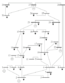
(a)

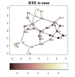
(b)

Figure 1: Motivating example: IEEE 30-bus system [45] (a) and its representation as a graph (b). The node color represents the state signal value.

The characteristics of the state estimation problem in power systems are as follows. First, the power flow equations are an up-to-a-constant function w.r.t. the state vector, $\theta$ [23], i.e. relative measurements, as described in Section V. Thus, the MSE cannot be used directly as a performance measure without the use of a reference bus (node). Additionally, it has recently been shown in [12, 11] that the state vector in power systems is a smooth graph signal w.r.t. the associated Laplacian matrix that is determined by the susceptances values. Thus, the GSP framework is well suited for PSSE, as shown, for example, in [11, 12] for addressing the problem of detection of false data injection attacks in power systems based on the GFT of the states.

III Laplacian-based WMSE estimation

Sampling and recovery of graph signals are fundamental tasks in GSP that have received considerable attention. In regular domains, signal recovery is usually performed based on the MSE criterion. However, the MSE may be limited for characterizing the performance of graph signal recovery since it ignores the structural relationship in the neighborhood of the graph signals [14, 15]. In this section, we suggest the use of the WMSE for graph signal recovery. The proposed WMSE measures the variation of the estimation error w.r.t. the underlying graphs. The rationale behind the WMSE as a difference-based criterion that fits various applications, its Dirichlet energy interpretation, and its graph frequency interpretation are discussed in Subsections III-1, III-2, and III-3, respectively.

In this paper, we suggest the use of the following matrix cost function for graph signal recovery:

$${\bf{C}}(\hat{{\mbox{\boldmath$\theta$}}},{\mbox{\boldmath$\theta$}})\stackrel{{\scriptstyle\triangle}}{{=}}{\bf{\Lambda}}^{\frac{1}{2}}{\bf{V}}^{T}(\hat{{\mbox{\boldmath$\theta$}}}-{\mbox{\boldmath$\theta$}})(\hat{{\mbox{\boldmath$\theta$}}}-{\mbox{\boldmath$\theta$}})^{T}{\bf{V}}{\bf{\Lambda}}^{\frac{1}{2}},$$ (6)

where ${\bf{V}}$ and ${\bf{\Lambda}}$ are defined in (1). The corresponding risk, which is the expected cost from (6), is the following WMSE:

$${\rm{E}}_{{\mbox{\boldmath{\scriptsize$\theta$}}}}[{\bf{C}}(\hat{{\mbox{\boldmath$\theta$}}},{\mbox{\boldmath$\theta$}})]={\bf{\Lambda}}^{\frac{1}{2}}{\bf{V}}^{T}{\text{MSE}}(\hat{{\mbox{\boldmath$\theta$}}},{\mbox{\boldmath$\theta$}}){\bf{V}}{\bf{\Lambda}}^{\frac{1}{2}},$$ (7)

where the MSE matrix is defined as:

$${\text{MSE}}(\hat{{\mbox{\boldmath$\theta$}}},{\mbox{\boldmath$\theta$}})\stackrel{{\scriptstyle\triangle}}{{=}}{\rm{E}}_{{\mbox{\boldmath{\scriptsize$\theta$}}}}[(\hat{{\mbox{\boldmath$\theta$}}}-{\mbox{\boldmath$\theta$}})(\hat{{\mbox{\boldmath$\theta$}}}-{\mbox{\boldmath$\theta$}})^{T}].$$ (8)

The proposed risk in (7) can be interpreted as a WMSE criterion [46, 43] with a positive semidefinite weighting matrix, ${\bf{\Lambda}}^{\frac{1}{2}}{\bf{V}}^{T}$. Different weights are assigned to the individual errors, where these weights are based on the graph topology. The Laplacian matrix, ${\bf{L}}$, which is used to determine these weights through ${\bf{\Lambda}}$ and ${\bf{V}}^{T}$, can be based on a physical network or on statistical dependency, such as a probabilistic graphical model that is obtained from historic, offline data.

The rationale behind this cost function, as well as some of its properties, are as follows:

III-1 Difference-based criterion

It is proved in Appendix A that the $(m,n)$th element of the matrix cost, ${\bf{C}}(\hat{{\mbox{\boldmath$\theta$}}},{\mbox{\boldmath$\theta$}})$, is

$${\bf{C}}_{m,n}(\hat{{\mbox{\boldmath$\theta$}}},{\mbox{\boldmath$\theta$}})\hskip 170.71652pt$$

$$={\bf{\Lambda}}^{\frac{1}{2}}_{m,m}{\bf{\Lambda}}^{\frac{1}{2}}_{n,n}\sum_{k=1}^{M}\sum_{l=1}^{M}{\bf{V}}_{k,m}{\bf{V}}_{l,n}(\epsilon_{k}-\epsilon_{m})(\epsilon_{l}-\epsilon_{n}),$$ (9)

where the estimation error at node $m$ is defined by

$$\epsilon_{m}\stackrel{{\scriptstyle\triangle}}{{=}}\hat{\theta}_{m}-\theta_{m},~{}m=1,\ldots,M.$$ (10)

The elements of the cost matrix in (III-1) imply that the proposed matrix cost function only takes into account the relative estimation errors of the differences between the error signals at different nodes. Thus, any translation of all errors by a vector $c{\bf{1}}$, would not change the matrix cost. This property reflects the fact that in various applications, such as control, power systems, and image processing [20, 21, 15, 8, 9, 22], graph signals are only a function of the differences between vertex values, and estimation can only be achieved up to a constant addend [23, 20, 21]. It should be noted that the derivation of (III-1) in Appendix A is based on the fact that $(\lambda_{1},{\bf{v}}_{1})=(0,\frac{1}{\sqrt{M}}{\bf{1}})$ is the smallest eigenvalue-eigenvector pair of ${\bf{L}}$. Thus, (III-1) does not hold for other forms of the Laplacians.

In addition, since for the Laplacian matrix $\lambda_{1}=0$, then ${\bf{\Lambda}}_{1,1}=\lambda_{1}=0$. By substituting this value in (III-1), we obtain

$${\bf{C}}_{m,n}(\hat{{\mbox{\boldmath$\theta$}}},{\mbox{\boldmath$\theta$}})=0,~{}{\text{if }}m=1{\text{ and{/}or }}n=1.$$ (11)

Therefore, minimization of the expected matrix cost, ${\rm{E}}_{\mbox{\boldmath{\scriptsize$\theta$}}}[{\bf{C}}(\hat{{\mbox{\boldmath$\theta$}}},{\mbox{\boldmath$\theta$}})]$, in the sense of positive semidefinite matrices, is equivalent to minimization of the submatrix ${\rm{E}}_{\mbox{\boldmath{\scriptsize$\theta$}}}[{\bf{C}}_{\mathcal{M}\setminus 1}(\hat{{\mbox{\boldmath$\theta$}}},{\mbox{\boldmath$\theta$}})]$.

III-2 Dirichlet energy interpretation

By substituting (1) in (6) and using the trace operator properties, it can be verified that the trace of ${\bf{C}}(\hat{{\mbox{\boldmath$\theta$}}},{\mbox{\boldmath$\theta$}})$ is given by

$${\text{Tr}}({\bf{C}}(\hat{{\mbox{\boldmath$\theta$}}},{\mbox{\boldmath$\theta$}}))=(\hat{{\mbox{\boldmath$\theta$}}}-{\mbox{\boldmath$\theta$}})^{T}{\bf{V}}{\bf{\Lambda}}{\bf{V}}^{T}(\hat{{\mbox{\boldmath$\theta$}}}-{\mbox{\boldmath$\theta$}})$$

$$=(\hat{{\mbox{\boldmath$\theta$}}}-{\mbox{\boldmath$\theta$}})^{T}{\bf{L}}(\hat{{\mbox{\boldmath$\theta$}}}-{\mbox{\boldmath$\theta$}}).\hskip 22.76228pt$$ (12)

By substituting ${\bf{L}}={\bf{D}}-{\bf{W}}$ in (III-2) it can be shown that

$${\text{Tr}}({\bf{C}}(\hat{{\mbox{\boldmath$\theta$}}},{\mbox{\boldmath$\theta$}}))=\frac{1}{2}\sum_{m=1}^{M}\sum_{k\in{\mathcal{N}}_{m}}{\bf{W}}_{m,k}(\epsilon_{k}-\epsilon_{m})^{2},$$ (13)

where ${\mathcal{N}}_{m}$ is the set of connected neighbors of node $m$, as defined in Definition 1.

The trace of the cost in (III-2) and (13) is the Dirichlet energy of the estimation error signal, ${\mbox{\boldmath$\epsilon$}}=\hat{{\mbox{\boldmath$\theta$}}}-{\mbox{\boldmath$\theta$}}$, w.r.t. the Laplacian matrix ${\bf{L}}$ [47, 31]. This smoothness measure, which is well known in spectral graph theory, quantifies how much the signal changes w.r.t. the variability encoded by the graph weights. Intuitively, since the weights are nonnegative, the graph Dirichlet energy in (III-2) shows that an estimator, $\hat{{\mbox{\boldmath$\theta$}}}$, is considered to be a “good estimator” if the error is a smooth signal and the error values are close to their neighbors’ values, as described on the right hand side (r.h.s.) of (13). Additionally, it can be seen from (13) that the proposed measure penalizes the squared differences of estimation errors proportionally to the weights of connections between them, $\{{\bf{W}}_{m,k}\}_{(m,k)\in{\xi}}$. This is due to the fact that the errors in highly-connected vertices with a large degree have more influence on subsequent processing than those of separated vertices and, thus, should be penalized more.

III-3 Graph frequency interpretation

By substituting the GFT operator from (2) in (6), we obtain the equivalent graph frequency cost function:

$${\bf{C}}(\hat{{\mbox{\boldmath$\theta$}}},{\mbox{\boldmath$\theta$}})={\bf{\Lambda}}^{\frac{1}{2}}(\hat{\tilde{{\mbox{\boldmath$\theta$}}}}-\tilde{{\mbox{\boldmath$\theta$}}})(\hat{\tilde{{\mbox{\boldmath$\theta$}}}}-\tilde{{\mbox{\boldmath$\theta$}}})^{T}{\bf{\Lambda}}^{\frac{1}{2}},$$ (14)

where $\hat{\tilde{{\mbox{\boldmath$\theta$}}}}\stackrel{{\scriptstyle\triangle}}{{=}}{\bf{V}}^{T}\hat{{\mbox{\boldmath$\theta$}}}$ can be interpreted as an estimator of $\tilde{{\mbox{\boldmath$\theta$}}}$. That is, the proposed matrix cost function penalizes the marginal estimation errors in the frequency domain, weighted by the associated eigenvalue. In particular, since for the Laplacian matrix $\lambda_{1}=0$, then ${\bf{\Lambda}}_{1,1}=0$ and $\hat{\tilde{\theta}}_{1}-\tilde{\theta}_{1}$, does not affect the cost function in (14). By applying the trace operator on (14), one obtains

$${\text{Tr}}({\bf{C}}(\hat{{\mbox{\boldmath$\theta$}}},{\mbox{\boldmath$\theta$}}))=\sum_{m=2}^{M}\lambda_{m}(\hat{\tilde{\theta}}_{m}-\tilde{\theta}_{m})^{2}.$$ (15)

III-4 Alternative cost function

It should be noted that the matrix cost function ${\bf{C}}(\hat{{\mbox{\boldmath$\theta$}}},{\mbox{\boldmath$\theta$}})$ from (6) can be straightforwardly modified according to the specific parameter estimation problem. For example, problem dimensionality can be reduced using only part of the graph frequencies, instead of the full Laplacian matrix, for the reconstruction of graph bandlimited signals. That is, we can use the cost matrix

$${\bf{\Lambda}}_{\mathcal{S},\mathcal{S}}^{\frac{1}{2}}{\bf{V}}_{\mathcal{M},\mathcal{S}}^{T}(\hat{{\mbox{\boldmath$\theta$}}}-{\mbox{\boldmath$\theta$}})(\hat{{\mbox{\boldmath$\theta$}}}-{\mbox{\boldmath$\theta$}})^{T}{\bf{V}}_{\mathcal{M},\mathcal{S}}{\bf{\Lambda}}_{\mathcal{S},\mathcal{S}}^{\frac{1}{2}},$$ (16)

where $\mathcal{S}\subseteq{\mathcal{M}}$ is a subset of the indices of the graph frequencies. In addition, the cost function in (6) can be extended to different smoothness measures, e.g. by using

$${\bf{\Lambda}}^{\frac{p}{2}}{\bf{V}}^{T}(\hat{{\mbox{\boldmath$\theta$}}}-{\mbox{\boldmath$\theta$}})(\hat{{\mbox{\boldmath$\theta$}}}-{\mbox{\boldmath$\theta$}})^{T}{\bf{V}}{\bf{\Lambda}}^{\frac{p}{2}},~{}p\geq 1.$$ (17)

Another class of matrix costs can be obtained by using the SVD of other forms of Laplacian, such as the random-walk Laplacian, and any general graph-shift operator (GSO), ${\bf{S}}$, which is an $M\times M$ matrix whose $(m,k)$th entry is zero for any nonadjacent vertices, $m$ and $k$. For example, in [15], the sum-of-squares errors between all connected vertices, i.e. a loss function that is based on weighting by the adjacency matrix of the network, has been proposed. Another alternative cost function can be defined based on different choices of GFT bases with variation operators, as described in Table 1 in [32]. In general, taking practical considerations into account, a cost function should capture the relevant errors meaningfully and, at the same time, be easily computed. An example for an alternative cost function is described for bandlimited graph signal recovery in Subsection VI-E.

IV Graph CRB

The CRB is a commonly-used lower bound on the MSE matrix from (8) of any unbiased estimator. In this section, a Cram$\acute{\text{e}}$r-Rao-type lower bound for graph-signal recovery, which is useful for performance analysis and system design in networks, is derived in Section IV-B. The proposed graph CRB is a lower bound on the WMSE from (7) of any unbiased estimator, where the unbiasedness w.r.t. the graph is defined in Section IV-A by using the concept of Lehmann unbiasedness.

IV-A Graph unbiasedness

Lehmann [37] proposed a generalization of the unbiasedness concept based on the chosen cost function for each scenario, which can be used for various cost functions (see, e.g. [48, 17, 17, 43]). The Lehmann unbiasedness definition for a matrix cost functions is defined as follows (p. 13 in [49]):

Definition 2.

The estimator, $\hat{{\mbox{\boldmath$\theta$}}}$, is said to be a uniformly unbiased estimator of $\theta$ in the Lehmann sense w.r.t. a general positive semidefinite matrix cost function, ${\bf{C}}(\hat{{\mbox{\boldmath$\theta$}}},{\mbox{\boldmath$\theta$}})$, if

$${\rm{E}}_{{\mbox{\boldmath{\scriptsize$\theta$}}}}[{\bf{C}}(\hat{{\mbox{\boldmath$\theta$}}},{\mbox{\boldmath$\eta$}})]\succeq{\rm{E}}_{{\mbox{\boldmath{\scriptsize$\theta$}}}}[{\bf{C}}(\hat{{\mbox{\boldmath$\theta$}}},{\mbox{\boldmath$\theta$}})],~{}\forall{\mbox{\boldmath$\eta$}},{\mbox{\boldmath$\theta$}}\in\Omega_{\mbox{\boldmath{\scriptsize$\theta$}}},$$ (18)

where $\Omega_{\mbox{\boldmath{\scriptsize$\theta$}}}$ is the parameter space.

The following proposition defines a sufficient condition for the graph unbiasedness of estimators in the Lehmann sense w.r.t. the Laplacian-based WMSE and under the linear parametric constraints.

Proposition 1.

If an estimator, $\hat{{\mbox{\boldmath$\theta$}}}$, satisfies

$${\bf{U}}^{T}{\bf{L}}{\rm{E}}_{{\mbox{\boldmath{\scriptsize$\theta$}}}}[\hat{{\mbox{\boldmath$\theta$}}}-{\mbox{\boldmath$\theta$}}]={\bf{0}},~{}\forall{\mbox{\boldmath$\theta$}}\in\Omega_{\mbox{\boldmath{\scriptsize$\theta$}}},$$ (19)

where $\Omega_{\mbox{\boldmath{\scriptsize$\theta$}}}$ is defined in (4), then, $\hat{{\mbox{\boldmath$\theta$}}}$ is an unbiased estimator of the graph signal, $\theta$, in the Lehmann sense, as defined in Definition 2, w.r.t. the weighted squared-error cost function from (6) and under the constrained set in (3).

Proof:

The proof is given in Appendix B. ∎

It can be seen that if an estimator has a zero mean bias, i.e. ${\rm{E}}_{{\mbox{\boldmath{\scriptsize$\theta$}}}}[\hat{{\mbox{\boldmath$\theta$}}}]-{\mbox{\boldmath$\theta$}}={\bf{0}}$, $\forall{\mbox{\boldmath$\theta$}}\in\Omega_{\mbox{\boldmath{\scriptsize$\theta$}}}$, then it satisfies (19), but not vice versa. Thus, the uniform graph unbiasedness condition is a weaker condition than requiring the mean-unbiasedness property. For example, since ${\bf{L}}{\bf{1}}={\bf{0}}$, the condition in (19) is oblivious to the estimation error of a constant bias over the graph, $c{\bf{1}}$, for any constant $c\in{\mathbb{R}}$, in contrast with mean unbiasedness. It can be seen that the graph unbiasedness in (19) is a function of the specific graph topology. In addition, the unbiasedness definition can be reformulated by using any matrix that spans the null space of ${\bf{G}}$, ${\mathcal{N}}({\bf{G}})$, instead of ${\bf{U}}$.

Special case 1.

For the case where no constraint is imposed, i.e. $K=0$, we have ${\bf{U}}={\bf{I}}_{M}$ and the condition in (19) is reduced to

$${\bf{V}}{\bf{\Lambda}}{\rm{E}}_{{\mbox{\boldmath{\scriptsize$\theta$}}}}[\hat{\tilde{{\mbox{\boldmath$\theta$}}}}-\tilde{{\mbox{\boldmath$\theta$}}}]={\bf{0}},~{}\forall\tilde{{\mbox{\boldmath$\theta$}}}\in{\mathbb{R}}^{M},$$ (20)

where we used the GFT operator from (2). The condition in (20) is equivalent to the requirement that for each nonzero eigenvalue, the bias in the frequency domain should be zero.

Another special case of the graph-unbiasedness for a bandlimited graph signal is discussed in Subsection VI-B.

In non-Bayesian estimation theory, two types of unbiasedness are usually considered: uniform unbiasedness at any point in the parameter space, and local unbiasedness, in which the estimator is assumed to be unbiased only in the vicinity of the parameter ${\mbox{\boldmath$\theta$}}_{0}$. By using the feasible directions of the constraint set, similar to the derivations in [44, 43], it can be shown that the local graph-unbiasedness conditions are as follows:

Definition 3.

Necessary conditions for an estimator $\hat{{\mbox{\boldmath$\theta$}}}:\Omega_{\bf{x}}\rightarrow{\mathbb{R}}^{M}$ to be a locally Lehmann-unbiased estimator in the vicinity of ${\mbox{\boldmath$\theta$}}_{0}\in\Omega_{\mbox{\boldmath{\scriptsize$\theta$}}}$ w.r.t. the WMSE are

$${\bf{U}}^{T}{\bf{L}}\left.{\rm{E}}_{{\mbox{\boldmath{\scriptsize$\theta$}}}}[\hat{{\mbox{\boldmath$\theta$}}}-{\mbox{\boldmath$\theta$}}]\right|_{{\mbox{\boldmath{\scriptsize$\theta$}}}={\mbox{\boldmath{\scriptsize$\theta$}}}_{0}}={\bf{0}}$$ (21)

and

$${\bf{U}}^{T}{\bf{L}}\left.\nabla_{{\mbox{\boldmath{\scriptsize$\theta$}}}}{\rm{E}}_{{\mbox{\boldmath{\scriptsize$\theta$}}}}[\hat{{\mbox{\boldmath$\theta$}}}-{\mbox{\boldmath$\theta$}}]\right|_{{\mbox{\boldmath{\scriptsize$\theta$}}}={\mbox{\boldmath{\scriptsize$\theta$}}}_{0}}{\bf{U}}={\bf{0}}.$$ (22)

IV-B Graph CRB

In the following, a novel graph CRB for the estimation of graph parameters is derived. Various low-complexity, distributive algorithms exist for graph signal recovery. The new bound is a useful tool for assessing their performance. The proposed graph CRB is a lower bound on the WMSE of local graph-unbiased estimators in the vicinity of $\theta$.

Theorem 1.

Let $\hat{{\mbox{\boldmath$\theta$}}}$ be a locally graph-unbiased estimator of $\theta$, as defined in Definition 3, and assume the following regularity conditions:

1. The operations of integration w.r.t. ${\bf{x}}$ and differentiation w.r.t. $\theta$ can be interchanged, as follows:

   $$\nabla_{{\mbox{\boldmath{\scriptsize$\theta$}}}}\int_{\Omega_{\bf{x}}}{\bf{g}}({\bf{x}},{\mbox{\boldmath$\theta$}})\,\mathrm{d}{\bf{x}}=\int_{\Omega_{\bf{x}}}\nabla_{{\mbox{\boldmath{\scriptsize$\theta$}}}}{\bf{g}}({\bf{x}},{\mbox{\boldmath$\theta$}})\,\mathrm{d}{\bf{x}},$$ (23)

   for any measurable function ${\bf{g}}({\bf{x}},{\mbox{\boldmath$\theta$}})$.

2. The Fisher information matrix (FIM),

   $${\bf{J}}({\mbox{\boldmath$\theta$}})\stackrel{{\scriptstyle\triangle}}{{=}}{\rm{E}}_{{\mbox{\boldmath{\scriptsize$\theta$}}}}\left[\nabla_{{\mbox{\boldmath{\scriptsize$\theta$}}}}^{T}\log f({\bf{x}};{\mbox{\boldmath$\theta$}})\nabla_{{\mbox{\boldmath{\scriptsize$\theta$}}}}\log f({\bf{x}};{\mbox{\boldmath$\theta$}})\right],$$ (24)

   is well defined and finite.

Then,

$${\rm{E}}_{{\mbox{\boldmath{\scriptsize$\theta$}}}}[{\bf{C}}(\hat{{\mbox{\boldmath$\theta$}}},{\mbox{\boldmath$\theta$}})]\succeq{\bf{B}}({\mbox{\boldmath$\theta$}}),~{}\forall{\mbox{\boldmath$\theta$}}\in\Omega_{\mbox{\boldmath{\scriptsize$\theta$}}},$$ (25)

where

$${\bf{B}}({\mbox{\boldmath$\theta$}})\stackrel{{\scriptstyle\triangle}}{{=}}{\bf{\Lambda}}^{\frac{1}{2}}{\bf{V}}^{T}{\bf{U}}({\bf{U}}^{T}{\bf{J}}({\mbox{\boldmath$\theta$}}){\bf{U}})^{\dagger}{\bf{U}}^{T}{\bf{V}}{\bf{\Lambda}}^{\frac{1}{2}}.$$ (26)

Equality in (25) is obtained iff the estimation error in the graph-frequency domain satisfies

$${\bf{\Lambda}}^{\frac{1}{2}}(\hat{\tilde{{\mbox{\boldmath$\theta$}}}}-\tilde{{\mbox{\boldmath$\theta$}}})={\bf{\Lambda}}^{\frac{1}{2}}{\bf{V}}^{T}{\bf{U}}\left({\bf{U}}^{T}{\bf{J}}({\mbox{\boldmath$\theta$}}){\bf{U}}\right)^{\dagger}{\bf{U}}^{T}\nabla_{{\mbox{\boldmath{\scriptsize$\theta$}}}}^{T}\log f({\bf{x}};{\mbox{\boldmath$\theta$}}),$$ (27)

$\forall{\mbox{\boldmath$\theta$}}\in\Omega_{\mbox{\boldmath{\scriptsize$\theta$}}}$.

Proof:

The proof is given in Appendix C. ∎

Similar to the explanations in Subsection III-1, it can be seen that the first row and column of the proposed matrix bound in (26), ${\bf{B}}({{\mbox{\boldmath$\theta$}}})$, is zero. Thus, in practice, we use the submatrix bound, ${\bf{B}}_{\mathcal{M}\setminus 1}({{\mbox{\boldmath$\theta$}}})$. Discussion of pseudo-inverse matrix bounds in the general case can be found, for example, in [50].

IV-B1 Relation with the constrained CRB (CCRB) on the MSE

The CCRB, which was originally presented in [41], is a lower bound on the MSE of $\chi$-unbiased estimators [43, 44] in constrained parameter estimation settings. The CCRB is especially suitable for the case of linear constraints [43] and it is attained asymptotically by the commonly-used constrained maximum likelihood (CML) estimator [51]. It can be verified that the proposed bound in (26) is a weighted version of the CCRB, i.e.

$${\bf{B}}({\mbox{\boldmath$\theta$}})={\bf{\Lambda}}^{\frac{1}{2}}{\bf{V}}^{T}{\bf{B}}_{\text{CCRB}}({\mbox{\boldmath$\theta$}}){\bf{V}}{\bf{\Lambda}}^{\frac{1}{2}},$$ (28)

where the CCRB is given by [42]

$${\bf{B}}_{\text{CCRB}}({\mbox{\boldmath$\theta$}})={\bf{U}}({\bf{U}}^{T}{\bf{J}}({\mbox{\boldmath$\theta$}}){\bf{U}})^{\dagger}{\bf{U}}^{T}.$$ (29)

This result stems from the fact that the performance criterion in this paper is a weighted version of the MSE with the structure described in (7). The equality condition of the CCRB holds iff [42, 41, 43, 44]

$$\hat{{\mbox{\boldmath$\theta$}}}-{\mbox{\boldmath$\theta$}}={\bf{U}}\left({\bf{U}}^{T}{\bf{J}}({\mbox{\boldmath$\theta$}}){\bf{U}}\right)^{\dagger}{\bf{U}}^{T}\nabla_{{\mbox{\boldmath{\scriptsize$\theta$}}}}^{T}\log f({\bf{x}};{\mbox{\boldmath$\theta$}}).$$ (30)

It can be verified that if there is a constrained-efficient estimator which satisfies (30), then it is also an estimator which satisfies (27), but not vice versa. The equality conditions of the graph signal recovery are less restrictive, since the error w.r.t. the zero-graph frequency can be neglected.

IV-B2 Graph CRB on the Dirichlet energy

The WMSE bound in Theorem 1 is a matrix bound. As such, it implies bounds on the marginal WMSE of each node and on submatrices that are related to subgraphs. In particular, by applying the trace operator on the bound from (25)-(26) and using the trace operator properties, (1), and (III-2), we obtain the associated graph CRB on the expected Dirichlet energy:

$${\rm{E}}_{\mbox{\boldmath{\scriptsize$\theta$}}}[(\hat{{\mbox{\boldmath$\theta$}}}-{\mbox{\boldmath$\theta$}})^{T}{\bf{L}}(\hat{{\mbox{\boldmath$\theta$}}}-{\mbox{\boldmath$\theta$}})]\geq{\text{Tr}}({\bf{B}}({\mbox{\boldmath$\theta$}}))\hskip 71.13188pt$$

$$={\text{Tr}}\left({\bf{L}}{\bf{U}}({\bf{U}}^{T}{\bf{J}}({\mbox{\boldmath$\theta$}}){\bf{U}})^{\dagger}{\bf{U}}^{T}\right).$$ (31)

For an unconstrained estimation problem, in which ${\bf{U}}={\bf{I}}_{M}$, the bound in (IV-B2) is reduced to

$${\rm{E}}_{\mbox{\boldmath{\scriptsize$\theta$}}}[(\hat{{\mbox{\boldmath$\theta$}}}-{\mbox{\boldmath$\theta$}})^{T}{\bf{L}}(\hat{{\mbox{\boldmath$\theta$}}}-{\mbox{\boldmath$\theta$}})]\geq{\text{Tr}}({\bf{B}}({\mbox{\boldmath$\theta$}}))={\text{Tr}}\left({\bf{L}}{\bf{J}}^{\dagger}({\mbox{\boldmath$\theta$}})\right).$$ (32)

IV-B3 Efficiency

Definition 4.

A graph-unbiased estimator, in the sense of Proposition 1, that achieves the graph CRB in Theorem 1 is said to be an efficient estimator on the graph ${\mathcal{G}}({\mathcal{M}},\xi,{\bf{W}})$.

Similar to the conventional theory on estimators’ efficiency, it can be shown that if there is an estimator which satisfies (27) and it is not a function of $\theta$, then this is an efficient estimator. Moreover, similar to the uniformly minimum variance unbiased estimator [52, p. 20], the graph-efficient estimator from Definition 4 is also the uniformly minimum risk unbiased estimator, i.e. an estimator that is uniformly graph-unbiased (i.e. it satisfies (19)), and achieves minimum WMSE, defined in (7). From the definition of ${\bf{L}}$, it can be verified that ${\bf{L}}^{T}{\bf{y}}={\bf{0}}$ iff ${\bf{y}}=c{\bf{1}}_{M}$, where $c$ is an arbitrary scalar. Thus, if $\hat{{\mbox{\boldmath$\theta$}}}_{e}$ is an efficient estimator, then any shifted estimator $\hat{{\mbox{\boldmath$\theta$}}}_{e}+c{\bf{1}}$, where $c\in{\mathbb{R}}$ is a constant, is also an efficient estimator, since it also satisfies (27) and is not a function of $\theta$.

In the following, the graph CRB, estimation methods, and sensor allocation based on the graph CRB are developed for the special cases: 1) linear Gaussian model with relative measurements (Section V); and 2) recovery of a bandlimited graph signal from corrupted measurements (Section VI).

V Example 1: Linear Gaussian model with relative measurements

In this section, we discuss the problem of estimating vector-valued node variables from noisy relative measurements. This problem arises in many network applications, such as localization in sensor networks and motion consensus [20, 21], synchronization of translations [33, 53], edge flows [15], and state estimation in power systems [10, 11, 12, 13], where the vector $\theta$ represents parameters such as positions, states, opinions, and voltages. The measurement sensor network in this model (i.e. the measurement graph) may be different from the physical network used in the WMSE cost in Subsection II-C. This model represents the fact that many cyber-physical systems consist of two interacting networks: an underlying physical system with topological structure and a sensor network topology that may be with a different topology. Similarly, in other real-life applications such as in genetics, there exist dual networks, with a physical-world network and a second network that represents the conceptual or statistical world [54]. Another example is in communication systems where the topology (local data passage) of internode communication may be different from the graphical model use to describe local dependency [39]. In general, the two topologies do not necessarily match. In this section, we use “bar” to denote the topology associated with the measurements and determined by the sensing approach in order to distinguish it from the topology used in the WMSE (“physical” topology or a topology that was generated from a-priori data), described above. Finally, in this section we consider a linear model. For completeness, the interested reader is referred to an example of the recovery of a nonlinear model with relative measurements in power systems that is described in [23].

V-A Model

We consider a noisy measurement of the weighted relative state of each edge, as follows:

$$h_{m,k}=\bar{w}_{m,k}(\theta_{m}-\theta_{k})+\nu_{m,k},~{}~{}~{}\forall(m,k)\in\bar{\xi},$$ (33)

where $\{\nu_{m,k}\}$, $\forall(m,k)\in\bar{\xi}$, $m>k$, is an i.i.d. Gaussian noise sequence with variance $\sigma^{2}$. The sequence $\{\bar{w}_{m,k}\}$, $\forall(m,k)\in\bar{\xi}$, contains positive weights that are given by the system parameters and is assumed to be known. We assume that the edge weights satisfy $\bar{w}_{k,m}=\bar{w}_{m,k}$. Thus, from symmetry, the measurement and the noise sequences satisfy $h_{k,m}=-h_{m,k}$ and $\nu_{k,m}=-\nu_{m,k}$, respectively, $\forall(m,k)\in\bar{\xi}$. In general, $\bar{\xi}$ and $\{\bar{w}_{m,k}\}$, that are associated with the measurements and determined by the sensing approach, are different from $\xi$ and $\{{w}_{m,k}\}$, that are based on the physical graph. The goal here is to estimate the state vector, ${\mbox{\boldmath$\theta$}}=[\theta_{1},\ldots,\theta_{M}]^{T}$, from the observations in (33). For example, this problem with the model in (33) where $w_{m,k}=1$, $\forall(m,k)\in\bar{\xi}$, is the problem of synchronization of translations from [33, 53] . Another example is PSSE in electrical networks, [10, 11, 13], as described in Section VII.

Let ${\mathcal{G}}({\mathcal{M}},\bar{\xi},\bar{{\bf{W}}})$ be defined as the measurement graph associated with the model in (33) over the same vertex set as in the “physical” graph, ${\mathcal{G}}({\mathcal{M}},\xi,{\bf{W}})$, which is used in (7). We assume that ${\mathcal{G}}({\mathcal{M}},\bar{\xi},\bar{{\bf{W}}})$ is a connected simple graph and define its associated Laplacian matrix, $\bar{{\bf{L}}}{\in{\mathbb{R}}^{M\times M}}$, with the elements

$$\bar{{\bf{L}}}_{m,k}=\left\{\begin{array}[]{lr}\sum_{k\in\bar{\mathcal{N}}_{m}}\bar{w}_{m,k}&{\text{if }}m=k\\ -\bar{w}_{m,k}&{\text{if }}(m,k)\in\bar{\xi}\\ 0&{\text{otherwise}}\end{array}\right.,$$ (34)

where, similar to Definition 1, $\bar{\mathcal{N}}_{m}=\{k\in{\mathcal{M}}:(m,k)\in\bar{\xi}\}$. In addition, let the matrix $\bar{{\bf{E}}}$ be the ${M\times|\bar{\xi}|}$ oriented incidence matrix of the graph ${\mathcal{G}}({\mathcal{M}},\bar{\xi},\bar{{\bf{W}}})$. Thus, each of the columns of $\bar{{\bf{E}}}$ has two nonzero elements, $1$ in the $m$th row and $-1$ in the $k$th row, representing an edge connecting nodes $m$ and $k$, where the sign is chosen arbitrarily [55]. Then, the model in (33) can be rewritten in a matrix form as follows:

$${\bf{x}}={\text{diag}}(\bar{{\bf{w}}})\bar{{\bf{E}}}^{T}{\mbox{\boldmath$\theta$}}+{\mbox{\boldmath$\nu$}},$$ (35)

where ${\bf{x}}$, $\bar{{\bf{w}}}$, and $\nu$ include the elements $\{h_{m,k}\}$, $\{\bar{w}_{m,k}\}$, $\{\nu_{m,k}\}$, respectively, $\forall(m,k)\in\bar{\xi}$, $m>k$, in the same order, and we used the symmetry in the model, i.e. the fact that $\bar{w}_{k,m}=\bar{w}_{m,k}$, $h_{k,m}=-h_{m,k}$, and $\nu_{k,m}=-\nu_{m,k}$. By multiplying (35) by $\bar{{\bf{E}}}$ from the left and using the fact that [55]

$$\bar{{\bf{L}}}=\bar{{\bf{E}}}{\text{diag}}(\bar{{\bf{w}}})\bar{{\bf{E}}}^{T},$$ (36)

we obtain

$$\bar{{\bf{E}}}{\bf{x}}=\bar{{\bf{L}}}{\mbox{\boldmath$\theta$}}+\bar{{\bf{E}}}{\mbox{\boldmath$\nu$}}.$$ (37)

Since $\{\nu_{m,k}\}$, $m>k$, is an i.i.d. Gaussian noise sequence with variance $\sigma^{2}$, then $\bar{{\bf{E}}}{\mbox{\boldmath$\nu$}}$ is a zero-mean Gaussian vector with a covariance matrix $\sigma^{2}\bar{{\bf{E}}}\bar{{\bf{E}}}^{T}$.

V-B Graph CRB and an efficient estimator

The log-likelihood function for the modified model in (37), after removing constant terms and by using $\bar{{\bf{L}}}^{T}=\bar{{\bf{L}}}$, is

$$\log f({\bf{x}};{\mbox{\boldmath$\theta$}})=-\frac{1}{2\sigma^{2}}(\bar{{\bf{E}}}{\bf{x}}-\bar{{\bf{L}}}{\mbox{\boldmath$\theta$}})^{T}(\bar{{\bf{E}}}\bar{{\bf{E}}}^{T})^{\dagger}(\bar{{\bf{E}}}{\bf{x}}-\bar{{\bf{L}}}{\mbox{\boldmath$\theta$}}).\hskip 17.07182pt$$ (38)

Thus, the gradient of (38) satisfies

$$\nabla_{{\mbox{\boldmath{\scriptsize$\theta$}}}}^{T}\log f({\bf{x}};{\mbox{\boldmath$\theta$}})=\frac{1}{\sigma^{2}}\bar{{\bf{L}}}(\bar{{\bf{E}}}\bar{{\bf{E}}}^{T})^{\dagger}\left(\bar{{\bf{E}}}{{\bf{x}}}-\bar{{\bf{L}}}{\mbox{\boldmath$\theta$}}\right).$$ (39)

The matrix $\bar{{\bf{E}}}\bar{{\bf{E}}}^{T}$ is a Laplacian matrix with $M$ nodes and equal unit weights for all edges. Thus, its pseudo-inverse is given by [56]

$$(\bar{{\bf{E}}}\bar{{\bf{E}}}^{T})^{\dagger}=\left(\bar{{\bf{E}}}\bar{{\bf{E}}}^{T}-\frac{1}{M}{\bf{1}}{\bf{1}}^{T}\right)^{-1}+\frac{1}{M}{\bf{1}}{\bf{1}}^{T}.$$ (40)

By substituting (40) in (39) and using the null-space property, $\bar{{\bf{L}}}{\bf{1}}={\bf{0}}$, one obtains

$$\nabla_{{\mbox{\boldmath{\scriptsize$\theta$}}}}^{T}\log f({\bf{x}};{\mbox{\boldmath$\theta$}})=\frac{1}{\sigma^{2}}\bar{{\bf{L}}}\left(\bar{{\bf{E}}}\bar{{\bf{E}}}^{T}-\frac{1}{M}{\bf{1}}{\bf{1}}^{T}\right)^{-1}\left(\bar{{\bf{E}}}{{\bf{x}}}-\bar{{\bf{L}}}{\mbox{\boldmath$\theta$}}\right).$$ (41)

Thus, the FIM from (24) for this case is given by

$${\bf{J}}({\mbox{\boldmath$\theta$}}) = \frac{1}{\sigma^{2}}\bar{{\bf{L}}}\left(\bar{{\bf{E}}}\bar{{\bf{E}}}^{T}-\frac{1}{M}{\bf{1}}{\bf{1}}^{T}\right)^{-1}\bar{{\bf{L}}}.$$ (42)

The FIM in (42) is a function of the graph topology via the Laplacian and the oriented incidence matrices. For the special case of unit weights, i.e. for $\bar{{\bf{L}}}=\bar{{\bf{E}}}\bar{{\bf{E}}}^{T}$, the FIM satisfies ${\bf{J}}({\mbox{\boldmath$\theta$}})=\frac{1}{\sigma^{2}}\bar{{\bf{L}}}$, which coincides with the result in [33].

It is shown in Appendix D that the pseudo-inverse of the FIM in (42) is given by

$${\bf{J}}^{\dagger}({\mbox{\boldmath$\theta$}})=\sigma^{2}\bar{{\bf{L}}}^{\dagger}\bar{{\bf{E}}}\bar{{\bf{E}}}^{T}\bar{{\bf{L}}}^{\dagger}.$$ (43)

By substituting (43) and ${\bf{U}}={\bf{I}}_{M}$ (since there are no constraints in the considered model) in (25)-(26), we obtain that the graph CRB for this case is

$${\rm{E}}_{{\mbox{\boldmath{\scriptsize$\theta$}}}}[{\bf{C}}(\hat{{\mbox{\boldmath$\theta$}}},{\mbox{\boldmath$\theta$}})]\succeq{\bf{B}}({\mbox{\boldmath$\theta$}})=\sigma^{2}{\bf{\Lambda}}^{\frac{1}{2}}{\bf{V}}^{T}\bar{{\bf{L}}}^{\dagger}\bar{{\bf{E}}}\bar{{\bf{E}}}^{T}\bar{{\bf{L}}}^{\dagger}{\bf{V}}{\bf{\Lambda}}^{\frac{1}{2}},$$ (44)

which is not a function of the specific values of $\theta$. By applying the trace operator on (44), we obtain the bound on the expected Dirichlet energy, which is

$${\rm{E}}_{\mbox{\boldmath{\scriptsize$\theta$}}}[(\hat{{\mbox{\boldmath$\theta$}}}-{\mbox{\boldmath$\theta$}})^{T}{\bf{L}}(\hat{{\mbox{\boldmath$\theta$}}}-{\mbox{\boldmath$\theta$}})]\geq{\text{Tr}}({\bf{B}}({\mbox{\boldmath$\theta$}}))=\sigma^{2}{\text{Tr}}(\bar{{\bf{E}}}^{T}\bar{{\bf{L}}}^{\dagger}{\bf{L}}\bar{{\bf{L}}}^{\dagger}\bar{{\bf{E}}}).$$ (45)

The graph CRBs are lower bounds on the WMSE and on the Dirichlet energy of any graph unbiased estimators, as defined for this unconstrained setting in (20) in Special case 1.

For the estimator, by substituting (39), (43), and ${\bf{U}}={\bf{I}}_{M}$ in (27), equality in (44) is obtained iff

$${\bf{\Lambda}}^{\frac{1}{2}}{\bf{V}}^{T}(\hat{{\mbox{\boldmath$\theta$}}}-{\mbox{\boldmath$\theta$}})={\bf{\Lambda}}^{\frac{1}{2}}{\bf{V}}^{T}\bar{{\bf{L}}}^{\dagger}\bar{{\bf{E}}}^{T}\bar{{\bf{E}}}\bar{{\bf{L}}}^{\dagger}\bar{{\bf{L}}}(\bar{{\bf{E}}}\bar{{\bf{E}}}^{T})^{\dagger}(\bar{{\bf{E}}}{{\bf{x}}}-\bar{{\bf{L}}}{\mbox{\boldmath$\theta$}}).$$ (46)

By using the properties of the Laplacian and incidence matrices, as well as its pseudo-inverse properties, it can be shown that $\bar{{\bf{E}}}^{T}\bar{{\bf{E}}}\bar{{\bf{L}}}^{\dagger}\bar{{\bf{L}}}(\bar{{\bf{E}}}\bar{{\bf{E}}}^{T})^{\dagger}\bar{{\bf{E}}}=\bar{{\bf{E}}}$ and $\bar{{\bf{E}}}^{T}\bar{{\bf{E}}}\bar{{\bf{L}}}^{\dagger}\bar{{\bf{L}}}(\bar{{\bf{E}}}\bar{{\bf{E}}}^{T})^{\dagger}\bar{{\bf{L}}}=\bar{{\bf{L}}}$. Thus, (46) implies the following condition for achievablity of the bound:

$${\bf{\Lambda}}^{\frac{1}{2}}{\bf{V}}^{T}\hat{{\mbox{\boldmath$\theta$}}} = {\bf{\Lambda}}^{\frac{1}{2}}{\bf{V}}^{T}\bar{{\bf{L}}}^{\dagger}\bar{{\bf{E}}}{{\bf{x}}}+{\bf{\Lambda}}^{\frac{1}{2}}{\bf{V}}^{T}({\bf{I}}_{M}-\bar{{\bf{L}}}^{\dagger}\bar{{\bf{L}}}){\mbox{\boldmath$\theta$}}$$ (47)

$$= {\bf{\Lambda}}^{\frac{1}{2}}{\bf{V}}^{T}\bar{{\bf{L}}}^{\dagger}\bar{{\bf{E}}}{{\bf{x}}}+\frac{1}{M}{\bf{\Lambda}}^{\frac{1}{2}}{{\bf{V}}}^{T}{\bf{1}}{\bf{1}}^{T}{\mbox{\boldmath$\theta$}}$$

$$= {\bf{\Lambda}}^{\frac{1}{2}}{\bf{V}}^{T}\bar{{\bf{L}}}^{\dagger}\bar{{\bf{E}}}{{\bf{x}}},$$

where the second equality is obtained by using the fact that for connected graphs there is only one zero eigenvalue of the Laplacian matrix, which is associated with the eigenvector ${\bf{v}}_{1}=\frac{1}{\sqrt{M}}{\bf{1}}$, and the last equality is obtained by using the Laplacian null-space property, ${\bf{\Lambda}}^{\frac{1}{2}}{{\bf{V}}}^{T}{\bf{1}}={\bf{0}}$. Since the estimator on the r.h.s. of (47) is not a function of $\theta$, then it is also an efficient estimator, in the sense of Definition 4. By using the null-space property ${{\bf{V}}}^{T}{\bf{1}}={\bf{0}}$, it can be verified that any estimator of the form

$$\hat{{\mbox{\boldmath$\theta$}}}=\bar{{\bf{L}}}^{\dagger}\bar{{\bf{E}}}{\bf{x}}+c{\bf{1}},$$ (48)

with an arbitrary scalar $c\in{\mathbb{R}}$, satisfies the equality condition in (47). Thus, the efficient estimator is not unique and the true signals, $\theta$, can be recovered up to a constant vector, $c{\bf{1}}$. This result is reasonable, since, with relative measurements alone, as given in the model in (33), determining the signal is possible only up to an additive constant [20, 21, 23].

V-C Sample allocation

In this subsection, we design a sample allocation rule for the sensing model from Subsection V-A based on solving an optimization problem that aims to minimize the graph CRB in (45). In this case, the graph CRB is achievable by the efficient estimator in (48) and is not a function of the unknown graph signal, $\theta$. Thus, minimizing the graph CRB in (45) will result in the minimum WMSE over graph unbiased estimators.

In many cases, the physical topology is known and is the one that is both used in the cost function in (7) and governs the measurement model in (33) for any edge that is measured. Thus, in the following we assume that the edge weights in (33) satisfy $\bar{w}_{m,k}={w}_{m,k}$, $\forall(m,k)\in\xi\bigcap\bar{\xi}$, and the sensors can be located only in existing edges of the physical network, where if $(m,k)\in\bar{\xi}$, then $(k,m)\in\bar{\xi}$. We assume a constrained amount of sensing resources, e.g. due to limited energy and communication budget. We thus state the sensor placement problem as follows:

Problem 1.

Given a graph ${\mathcal{G}}({\mathcal{M}},\xi,{\bf{W}})$, find the smallest subset $\bar{\xi}\subset{\xi}$ such that the graph signal, $\theta$, can be correctly recovered (up-to-a-constant) by the measurements on $\bar{\xi}$ and the graph CRB from (45), $\sigma^{2}{\text{Tr}}(\bar{{\bf{E}}}^{T}\bar{{\bf{L}}}^{\dagger}{\bf{L}}\bar{{\bf{L}}}^{\dagger}\bar{{\bf{E}}})$, is minimized, where $\bar{w}_{m,k}={w}_{m,k}$, $\forall(m,k)\in\xi\bigcap\bar{\xi}$.

The requirement of correct graph signal recovery in Problem 1 is defined as recovery up to a constant vector, $c{\bf{1}}$, which is an inherent ambiguity with relative measurements. In order to correctly reconstruct the full graph signal by the estimator from (48) up-to-a-constant, we need to have ${\text{rank}}(\bar{{\bf{L}}})=M-1$. That is, for each node, $m\in M$, we need to have at least one edge in $\bar{\xi}$ which is associated with this node. It can be shown that this condition for unique up-to-a-constant recovery is that $\bar{\xi}$ is a spanning tree of ${\mathcal{G}}({\mathcal{M}},\xi,{\bf{W}})$ [57]. Thus, Problem 1 is equivalent to the following optimization problem.

Problem 2.

Given a graph ${\mathcal{G}}({\mathcal{M}},\xi,{\bf{W}})$, find the Laplacian matrix $\bar{{\bf{L}}}^{*}$ such that

$$\bar{{\bf{L}}}^{*}=\arg\min_{\bar{{\bf{L}}}}{\text{Tr}}(\bar{{\bf{L}}}^{\dagger}\bar{{\bf{E}}}\bar{{\bf{E}}}^{T}\bar{{\bf{L}}}^{\dagger}{\bf{L}}),~{}~{}{\text{such that }}\bar{{\bf{L}}}\in S_{T}({\mathcal{G}}),$$ (49)

where $S_{T}({\mathcal{G}})$ is the set of spanning trees of ${\mathcal{G}}({\mathcal{M}},\xi,{\bf{W}})$.

If $\bar{{\bf{L}}}$ is a spanning tree of a connected (loopless) graph, then it can be seen that its oriented incidence matrix, $\bar{{\bf{E}}}$, has $M-1$ linearly independent columns. Thus, $\bar{{\bf{E}}}^{T}(\bar{{\bf{E}}}\bar{{\bf{E}}}^{T})^{\dagger}\bar{{\bf{E}}}=\bar{{\bf{E}}}^{\dagger}\bar{{\bf{E}}}={\bf{I}}_{M-1}$ and by substituting (36), we obtain that for spanning trees

$$\bar{\bar{{\bf{L}}}}\stackrel{{\scriptstyle\triangle}}{{=}}\bar{{\bf{L}}}(\bar{{\bf{E}}}\bar{{\bf{E}}}^{T})^{\dagger}\bar{{\bf{L}}}=\bar{{\bf{E}}}{\text{diag}}(\bar{{\bf{w}}})\bar{{\bf{E}}}^{T}(\bar{{\bf{E}}}\bar{{\bf{E}}}^{T})^{\dagger}\bar{{\bf{E}}}{\text{diag}}(\bar{{\bf{w}}})\bar{{\bf{E}}}^{T}$$

$$=\bar{{\bf{E}}}{\text{diag}}(\bar{{\bf{w}}}){\text{diag}}(\bar{{\bf{w}}})\bar{{\bf{E}}}^{T}.\hskip 110.96556pt$$ (50)

That is, $\bar{\bar{{\bf{L}}}}$ is also a Laplacian matrix of a spanning tree of ${\bf{L}}$ with the weights $\{{w}_{m,k}^{2}\}$, $\forall(m,k)\in\bar{\xi}$, and the optimization from (49) is reduced to

Problem 3.

Given a graph ${\mathcal{G}}({\mathcal{M}},\xi,{\bf{W}})$, find the Laplacian matrix $\bar{\bar{{\bf{L}}}}^{*}$ such that

$$\min_{\bar{\bar{{\bf{L}}}}}{\text{Tr}}(\bar{\bar{{\bf{L}}}}^{\dagger}{\bf{L}}),~{}~{}{\text{such that }}\bar{{\bf{L}}}\in S_{T}({\mathcal{G}}),$$ (51)

where $\bar{\bar{{\bf{L}}}}=\bar{{\bf{E}}}{\text{diag}}(\bar{{\bf{w}}}){\text{diag}}(\bar{{\bf{w}}})\bar{{\bf{E}}}^{T}$ and ${\bar{{\bf{L}}}}=\bar{{\bf{E}}}{\text{diag}}(\bar{{\bf{w}}})\bar{{\bf{E}}}^{T}$.

It is shown in [58] that

$${\text{Tr}}({\bar{{\bf{L}}}}^{\dagger}{\bf{L}})=st_{{\bar{{\bf{L}}}}}({\bf{L}}),$$ (52)

where $st_{{\bar{{\bf{L}}}}}({\bf{L}})$ is the total stretch of the graph ${\mathcal{G}}({\mathcal{M}},\xi,{\bf{W}})$ w.r.t. the spanning tree represented by ${\bar{{\bf{L}}}}$. Total stretch is a parameter used to measure the quality of a spanning tree in terms of distance preservation and can represent the average effective resistance [58, 59]. The objective function in Problem 3 is the $\ell_{p=\frac{1}{2}}$ total stretch of the graph ${\mathcal{G}}({\mathcal{M}},\xi,{\bf{W}})$, i.e. the total stretch from (52) after taking the $p=\frac{1}{2}$ power of the weights of the edges [60]. Thus, the problem of finding the minimum graph CRB is equivalent to the problem of finding a spanning tree with the minimum average $\ell_{p=\frac{1}{2}}$ stretch, which is a classical problem in network design, graph theory, and discrete mathematics. Although this problem in general is an NP-hard problem, it was shown that a standard maximum weight spanning tree algorithm [61] yields good results in practice [62]. Thus, in this paper we solve the sensor allocation problem in Problem 3 by finding the maximum weight spanning tree of ${\mathcal{G}}({\mathcal{M}},\xi,{\bf{W}}^{2})$, which is one of the fundamental problems of algorithmic graph theory and can be solved by existing algorithms in near-linear time [61, 63].

VI Example 2: Bandlimited graph signal recovery

In this section, we consider the problem of signal recovery from noisy, corrupted, and incomplete measurements, under the constraint of bandlimited graph signals [64, 65]. In Subsection VI-A we present the model assumed in this section. The graph CRB and Lehmann unbiasedness are developed in Subsection VI-B and sensor allocation which uses the graph CRB as an objective function is discussed in Subsection VI-C. An efficient estimator for the Gaussian case is presented in Subsection VI-D. Finally, in Subsection VI-E we demonstrate the use of an alternative cost function, which does not enforce strictly bandlimited constraints.

VI-A Model

We assume the following measurement model:

$${\bf{x}}={\bf{M}}({\mbox{\boldmath$\theta$}}+{\bf{w}}),$$ (53)

where $\theta$ is an unknown signal, ${\bf{w}}$ is a noise vector with zero mean and a known distribution, and ${\bf{M}}\in[0,1]^{D\times M}$ is a binary mask matrix with $D\leq M$. The mask matrix, ${\bf{M}}$, may indicate missing data, i.e. the indicator matrix for the missing values [66], removing data which is irrelevant for a specific task [67, 68], as well as representing any interpolation, filtering, and normalization approaches [64]. The task is to recover the true signal, $\theta$, based on the accessible measurement vector, ${\bf{x}}$. Signal recovery from inaccessible and corrupted measurements requires additional knowledge of signal properties. In GSP, a widely-used assumption is that the signal of interest, $\theta$, is a graph-bandlimited signal [3, 2, 4], i.e. its GFT, $\tilde{{\mbox{\boldmath$\theta$}}}$, defined in (2), is a $R$-sparse vector. Here we assume a graph low-frequency signal defined as follows:

Definition 5.

A graph signal ${\mbox{\boldmath$\theta$}}\in{\mathbb{R}}^{M}$ is bandlimited w.r.t. a GFT basis ${\bf{V}}$, as defined in (2), with bandwidth $R$ when

$$\tilde{\theta}_{m}=0,~{}~{}~{}m=R+1,\ldots,M.$$ (54)

The condition in (54) can be represented as the linear constraint from (3) with

$${\bf{G}}={\bf{Q}}{\bf{V}}^{T}~{}{\text{and }}{\bf{a}}={\bf{0}}_{(M-R)\times 1},$$ (55)

where ${\bf{Q}}$ is an $(M-R)\times M$ matrix of the form $\ {\bf{Q}}=\left[{\bf{0}}_{(M-R)\times R},{\bf{I}}_{M-R}\right]$. Thus, a null-space matrix ${\bf{U}}$, defined in (5), can be chosen to be ${\bf{U}}={\bf{V}}\bar{{\bf{Q}}}$, where $\bar{{\bf{Q}}}=\left[\begin{array}[]{c}{\bf{I}}_{R}\\ {\bf{0}}_{(M-R)\times R}\end{array}\right]$.

VI-B Graph CRB and Lehmann unbiasedness

By substituting the model from Subsection VI-A in (19) it can be verified that in this case an estimator, $\hat{{\mbox{\boldmath$\theta$}}}$, is a Lehmann-unbiased estimator of $\theta$ under the constrained set in (54) iff

$$\bar{{\bf{Q}}}^{T}{\bf{V}}^{T}{\bf{\Lambda}}^{\frac{1}{2}}{\bf{V}}^{T}{\rm{E}}_{{\mbox{\boldmath{\scriptsize$\theta$}}}}[\hat{{\mbox{\boldmath$\theta$}}}-{\mbox{\boldmath$\theta$}}]={\bf{0}},~{}\forall{\mbox{\boldmath$\theta$}}\in\Omega_{\mbox{\boldmath{\scriptsize$\theta$}}}^{R},$$ (56)

where $\Omega_{\mbox{\boldmath{\scriptsize$\theta$}}}^{R}$ is the subspace of $R$-bandlimited graph signals that satisfy Definition (5). By using the GFT operator from (2), as well as the fact that $\lambda_{1}=0$, it can be verified that the unbiasedness condition in (56) is equivalent to requiring that

$${\rm{E}}_{{\mbox{\boldmath{\scriptsize$\theta$}}}}[\hat{\tilde{\theta}}_{m}-\tilde{\theta}_{m}]=0,~{}~{}~{}2\leq m\leq R.$$ (57)

The condition in (57) reflects the fact that the high graph frequencies are known to be zero for a $R$-bandlimited graph signal, and, thus, there is no need for an unbiasedness condition on frequencies higher than $R$. In addition, since the proposed cost is oblivious to the estimation error of a constant bias over the graph, $c{\bf{1}}$, then the estimator of the first graph frequency, $\hat{\tilde{\theta}}_{1}$, can also have an arbitrary bias.

By substituting ${\bf{U}}={\bf{V}}\bar{{\bf{Q}}}$, ${\bf{V}}^{T}{\bf{V}}={\bf{I}}$, and the model from (53) in (26), we obtain that the proposed graph CRB for graph bandlimited signals is given by

$${\bf{B}}({\mbox{\boldmath$\theta$}})={\bf{\Lambda}}^{\frac{1}{2}}\bar{{\bf{Q}}}\left(\bar{{\bf{Q}}}^{T}{\bf{V}}^{T}{\bf{M}}^{T}{\bf{J}}({\bf{M}}{\mbox{\boldmath$\theta$}}){\bf{M}}{\bf{V}}\bar{{\bf{Q}}}\right)^{\dagger}\bar{{\bf{Q}}}^{T}{\bf{\Lambda}}^{\frac{1}{2}},$$ (58)

where according to (24), ${\bf{J}}({\bf{M}}{\mbox{\boldmath$\theta$}})\in{\mathbb{R}}^{D\times D}$ is the FIM w.r.t. the unknown parameter vector ${\bf{M}}{\mbox{\boldmath$\theta$}}$. Thus, by a reparametrization of the FIM, it can be seen that ${\bf{J}}({\mbox{\boldmath$\theta$}})={\bf{M}}^{T}{\bf{J}}({\bf{M}}{\mbox{\boldmath$\theta$}}){\bf{M}}$.

Since ${\bf{\Lambda}}_{1,1}=0$, and due to the structure of $\bar{{\bf{Q}}}$, the first row and the last $M-R$ rows of ${\bf{\Lambda}}^{\frac{1}{2}}\bar{{\bf{Q}}}$ are zero rows. Thus, the relevant bound in (58) is the submatrix ${\bf{B}}_{\mathcal{M}\setminus 1}({\mbox{\boldmath$\theta$}})$, which deploys a bound in the estimation error associated with the low graph frequencies. As a result, by substituting (1) and (5) in (58), applying the trace operator on the result and using its properties, as well as the definition of $\bar{{\bf{Q}}}$, and under the assumption that $R\leq D$, we obtain that the trace graph CRB is given by

$${\text{Tr}}({\bf{B}}({\mbox{\boldmath$\theta$}}))=\sum_{m=2}^{R}\lambda_{m}\left[({\bf{V}}_{\mathcal{M},\mathcal{R}}^{T}{\bf{M}}^{T}{\bf{J}}({\bf{M}}{\mbox{\boldmath$\theta$}}){\bf{M}}{\bf{V}}_{\mathcal{M},\mathcal{R}})^{-1}\right]_{m,m},$$ (59)

where $\mathcal{R}=\{1,\ldots,R\}$. According to (IV-B2), (59) is a lower bound on the expected Dirichlet energy. It can be seen that a necessary and sufficient condition for a unique up-to-a-constant reconstruction of a graph bandlimited signal as defined in Definition (5), i.e. the reconstruction of $\tilde{\theta}_{m}$, $m=2,\ldots,R$, is that ${\text{rank}}({\bf{V}}_{\mathcal{M},\mathcal{R}}^{T}{\bf{M}}^{T}{\bf{J}}({\bf{M}}{\mbox{\boldmath$\theta$}}){\bf{M}}{\bf{V}}_{\mathcal{M},\mathcal{R}})=R$, which is determined by the properties of the matrix ${\bf{M}}$.

For the special case where ${\bf{M}}$ is a sampling matrix associated with the subset of nodes ${\mathcal{S}}$, i.e. it satisfies ${\bf{M}}_{\mathcal{D},{\mathcal{S}}}={\bf{I}}_{{\mathcal{S}}}$, ${\bf{M}}_{\mathcal{D},{\mathcal{S}}^{c}}={\bf{0}}$, $\mathcal{D}=\{1,\ldots,D\}$, and $D=|{\mathcal{S}}|$, then, according to the model in (53), ${\bf{x}}={\mbox{\boldmath$\theta$}}_{\mathcal{S}}+{\bf{w}}_{\mathcal{S}}$. Thus, ${\bf{M}}{\bf{V}}_{\mathcal{M},\mathcal{R}}={\bf{V}}_{\mathcal{S},\mathcal{R}}$ and (59) is reduced to

$${\text{Tr}}({\bf{B}}({\mbox{\boldmath$\theta$}}))=\sum\nolimits_{m=2}^{R}\lambda_{m}\left[({\bf{V}}_{\mathcal{S},\mathcal{R}}^{T}{\bf{J}}({\mbox{\boldmath$\theta$}}_{\mathcal{S}}){\bf{V}}_{{\mathcal{S}},\mathcal{R}})^{-1}\right]_{m,m}.$$ (60)

The r.h.s. of (60) demonstrates the fact that while we only have access to information on a subset of the states, ${\mbox{\boldmath$\theta$}}_{\mathcal{S}}$, we still have a well-defined estimator of the full vector $\theta$ as long as ${\bf{V}}_{\mathcal{S},\mathcal{R}}^{T}{\bf{J}}({\mbox{\boldmath$\theta$}}_{\mathcal{S}}){\bf{V}}_{{\mathcal{S}},\mathcal{R}}$ is a non-singular matrix.

Similar to the derivation of (60), by substituting ${\bf{U}}={\bf{V}}\bar{{\bf{Q}}}$, ${\bf{V}}^{T}{\bf{V}}={\bf{I}}$, and the model from (53) with ${\bf{M}}_{\mathcal{D},{\mathcal{S}}}={\bf{I}}_{{\mathcal{S}}}$ and ${\bf{M}}_{\mathcal{D},{\mathcal{S}}^{c}}={\bf{0}}$, in (29), we obtain that the trace CCRB for graph bandlimited signals is given by

$${\text{Tr}}\left({\bf{B}}_{\text{CCRB}}({\mbox{\boldmath$\theta$}})\right)={\text{Tr}}\left(\left(\bar{{\bf{Q}}}^{T}{\bf{V}}^{T}{\bf{M}}^{T}{\bf{J}}({\mbox{\boldmath$\theta$}}_{\mathcal{S}}){\bf{M}}{\bf{V}}\bar{{\bf{Q}}}\right)^{-1}\right)$$

$$=\sum_{m=1}^{R}\left[({\bf{V}}_{\mathcal{S},\mathcal{R}}^{T}{\bf{J}}({\mbox{\boldmath$\theta$}}_{\mathcal{S}}){\bf{V}}_{\mathcal{S},\mathcal{R}})^{-1}\right]_{m,m},$$ (61)

under the assumption that ${\bf{V}}_{\mathcal{S},\mathcal{R}}^{T}{\bf{J}}({\mbox{\boldmath$\theta$}}_{\mathcal{S}}){\bf{V}}_{\mathcal{S},\mathcal{R}}$ is a non-singular matrix. Thus, the CCRB is not affected by the eigenvalues of the Laplacian matrix (i.e. by the graph frequencies). For the special case of an i.i.d. Gaussian model, i.e. when ${\bf{J}}({\mbox{\boldmath$\theta$}})=\frac{1}{\sigma^{2}}{\bf{I}}$, the CCRB in (VI-B) satisfies

$${\text{Tr}}\left({\bf{B}}_{\text{CCRB}}({\mbox{\boldmath$\theta$}})\right)=\sigma^{2}{\text{Tr}}\left(({\bf{V}}_{\mathcal{S},\mathcal{R}}^{T}{\bf{V}}_{\mathcal{S},\mathcal{R}})^{-1}\right).$$ (62)

The conventional CCRB on the r.h.s. of (62) has been used as an objective function for graph sampling of bandlimited graph signals in [32], where this policy is called A-optimal design (up to a multiplication by $\sigma^{2}$).

VI-C Sensor allocation

The graph CRB in (60) allows us to define a criterion for sampling set selection. We thus state the sensor placement problem as follows:

Problem 4.

Given a graph ${\mathcal{G}}({\mathcal{M}},\xi,{\bf{W}})$, a cutoff frequency, $\lambda_{R}$, and a number of sensors $D$, find the subset of nodes (sensor placements) $\mathcal{S}^{*}$ such that all $R$-bandlimited signals can be uniquely recovered from their samples on this subset and the worst-case graph CRB from (60) is minimized, i.e.

$$\mathcal{S}^{*}=\arg\min_{\mathcal{S}:|\mathcal{S}|=D}\max_{{\mbox{\boldmath{\scriptsize$\theta$}}}\in\Omega_{\mbox{\boldmath\tiny$\theta$}}^{R}}\\ \sum_{m=2}^{R}\lambda_{m}\left[({\bf{V}}_{\mathcal{S},\mathcal{R}}^{T}{\bf{J}}({\mbox{\boldmath$\theta$}}_{\mathcal{S}}){\bf{V}}_{\mathcal{S},\mathcal{R}})^{-1}\right]_{m,m}.$$

In order for this problem to be well defined, we should consider only subsets such that ${\bf{V}}_{\mathcal{S},\mathcal{R}}^{T}{\bf{J}}({\mbox{\boldmath$\theta$}}_{\mathcal{S}}){\bf{V}}_{\mathcal{S},\mathcal{R}}$ is a full rank matrix. In particular, we require $D\geq R$. Since finding the optimal set in Problem 4 is an NP-hard problem, a greedy algorithm is described in Algorithm 1. At each iteration of this algorithm we remove the node that maximally increases the graph CRB in (60) (maximized w.r.t. $\theta$), until we obtain the subset $\mathcal{S}\subset{\mathcal{M}}$ with cardinality $D$. The greedy approach removes one sample at each iteration rather than adding one sensor at a time in order for the matrix ${\bf{V}}_{\mathcal{L}^{(i)}\setminus w,\mathcal{R}}^{T}{\bf{J}}({\mbox{\boldmath$\theta$}}_{\mathcal{L}^{(i)}\setminus w}){\bf{V}}_{\mathcal{L}^{(i)}\setminus w,\mathcal{R}}$ from the r.h.s. of (4) to be a non-singular matrix at each step. The complexity of this greedy approach can be reduced even further by applying methods with reduced complexity (see, e.g. [69, 70, 71, 72]).

Input:1) Laplacian matrix, ${\bf{L}}={\bf{V}}{\bf{\Lambda}}{\bf{V}}^{T}$, 2) number of sensors $D\geq R$, and 3) cutoff frequency, $R$
Output: Subset of sensors, $\mathcal{S}$

1:  Initialize the set of available locations, $\mathcal{L}^{(0)}={\mathcal{M}}$

2:  Initialize iteration index, $i=0$

3:  while $|\mathcal{L}^{(i)}|>M-D$ do

4:     Find the optimal node to remove:

$$w=\arg\min_{w\in{\mathcal{L}}^{(i)}}\max_{{\mbox{\boldmath{\scriptsize$\theta$}}}\in\Omega_{\mbox{\boldmath\tiny$\theta$}}^{R}}\sum\nolimits_{m=2}^{R}\lambda_{m}\hskip 71.13188pt$$

$$\times\left[({\bf{V}}_{\mathcal{L}^{(i)}\setminus w,\mathcal{R}}^{T}{\bf{J}}({\mbox{\boldmath$\theta$}}_{\mathcal{L}^{(i)}\setminus w}){\bf{V}}_{\mathcal{L}^{(i)}\setminus w,\mathcal{R}})^{-1}\right]_{m,m}$$ (63)

5:     Update the available locations, $\mathcal{L}^{(i)}\leftarrow\mathcal{L}^{(i-1)}\setminus w$, and the iteration index, $i\leftarrow i+1$

6:  end while

7:  Update the set of removed locations: $\mathcal{S}=\mathcal{M}\setminus\mathcal{L}^{(i)}$

Algorithm 1 Sensor allocation for bandlimited graph signals

VI-D Efficient estimator for the Gaussian case

The CML estimator of $\tilde{{\mbox{\boldmath$\theta$}}}$ is obtained by maximizing the log-likelihood function of the model in (53) under the constraint in (54). Then, by using the invariance property of the ML estimator [52], the CML estimator of $\theta$ is given by $\hat{{{\mbox{\boldmath$\theta$}}}}^{\text{CML}}={\bf{V}}\hat{\tilde{{\mbox{\boldmath$\theta$}}}}$. In the following, we develop an efficient estimator for the special case of Gaussian noise, which is also the CML estimator in this case. Thus, in the following, ${\bf{w}}$ is zero-mean Gaussian noise with a known covariance matrix, $\Sigma$, and, thus, (p. 47, [52])

$${\bf{J}}({\mbox{\boldmath$\theta$}})={\bf{M}}^{T}({\bf{M}}{\mbox{\boldmath$\Sigma$}}{\bf{M}}^{T})^{-1}{\bf{M}}.$$ (64)

By substituting ${\bf{U}}={\bf{V}}\bar{{\bf{Q}}}$ and the model from (53) in (27) and using ${\bf{V}}^{T}{\bf{V}}={\bf{I}}$, we obtain

$${\bf{\Lambda}}^{\frac{1}{2}}(\hat{\tilde{{\mbox{\boldmath$\theta$}}}}-\tilde{{\mbox{\boldmath$\theta$}}})={\bf{\Lambda}}^{\frac{1}{2}}\bar{{\bf{Q}}}\left(\bar{{\bf{Q}}}^{T}{\bf{V}}^{T}{\bf{M}}^{T}({\bf{M}}{\mbox{\boldmath$\Sigma$}}{\bf{M}}^{T})^{-1}{\bf{M}}{\bf{V}}\bar{{\bf{Q}}}\right)^{\dagger}$$

$$\times\bar{{\bf{Q}}}^{T}{\bf{V}}^{T}{\bf{M}}^{T}({\bf{M}}{\mbox{\boldmath$\Sigma$}}{\bf{M}}^{T})^{-1}\left({\bf{x}}-{\bf{M}}{\bf{V}}\tilde{{\mbox{\boldmath$\theta$}}}\right),$$ (65)

$\forall{\mbox{\boldmath$\theta$}}\in\Omega_{\mbox{\boldmath{\scriptsize$\theta$}}}^{R}$, where we use ${\bf{V}}^{T}{\bf{V}}={\bf{I}}_{M}$. Under the assumption that $\tilde{{\mbox{\boldmath$\theta$}}}$ is a $R$-bandlimited graph signal as defined in Definition 5 and that ${\text{rank}}({\bf{M}}{\bf{V}})=R$, it can be verified that

$$\hat{\tilde{{\mbox{\boldmath$\theta$}}}}=\bar{{\bf{Q}}}\left(\bar{{\bf{Q}}}^{T}{\bf{V}}^{T}{\bf{M}}^{T}({\bf{M}}{\mbox{\boldmath$\Sigma$}}{\bf{M}}^{T})^{-1}{\bf{M}}{\bf{V}}\bar{{\bf{Q}}}\right)^{\dagger}$$

$$\times\bar{{\bf{Q}}}^{T}{\bf{V}}^{T}{\bf{M}}^{T}({\bf{M}}{\mbox{\boldmath$\Sigma$}}{\bf{M}}^{T})^{-1}{\bf{x}}\hskip 42.67912pt$$ (66)

satisfies the efficiency condition in (VI-D). By using the definition of $\bar{{\bf{Q}}}$, the estimator from (VI-D) can be written as

$$\hat{\tilde{{\mbox{\boldmath$\theta$}}}}_{\mathcal{R}}=\left(\bar{{\bf{Q}}}^{T}{\bf{V}}^{T}{\bf{M}}^{T}({\bf{M}}{\mbox{\boldmath$\Sigma$}}{\bf{M}}^{T})^{-1}{\bf{M}}{\bf{V}}\bar{{\bf{Q}}}\right)^{\dagger}$$

$$\times\bar{{\bf{Q}}}^{T}{\bf{V}}^{T}{\bf{M}}^{T}({\bf{M}}{\mbox{\boldmath$\Sigma$}}{\bf{M}}^{T})^{-1}{\bf{x}}\hskip 28.45274pt$$ (67)

$$\hat{\tilde{{\mbox{\boldmath$\theta$}}}}_{\mathcal{M}\setminus\mathcal{R}}={\bf{0}}.\hskip 120.92421pt$$ (68)

Since $\hat{\tilde{{\mbox{\boldmath$\theta$}}}}$ is also the CML estimator of $\tilde{{\mbox{\boldmath$\theta$}}}$, then, by using the invariance property and (VI-D)-(68), the CML estimator of $\theta$ is given by $\hat{{{\mbox{\boldmath$\theta$}}}}^{\text{CML}}={\bf{V}}\hat{\tilde{{\mbox{\boldmath$\theta$}}}}$. Once the full-rank assumption of $\bar{{\bf{Q}}}^{T}{\bf{V}}^{T}{\bf{M}}^{T}({\bf{M}}{\mbox{\boldmath$\Sigma$}}{\bf{M}}^{T})^{-1}{\bf{M}}{\bf{V}}\bar{{\bf{Q}}}$ is satisfied, we can find a sampling operator to achieve perfect recovery for a given $M$.

VI-E Alternative approach for bandlimited graph signal recovery

In Subsections VI-A-VI-D we present the estimation approach that aims to minimize the WMSE from (7) under the strict constraints of zero high graph frequencies from (54). In this subsection we present an alternative approach for bandlimited graph signal recovery based on minimizing the WMSE only over the low graph frequencies, and without constraints. That is, we use the expected cost function from (16) with the frequency band $\mathcal{S}=\{1,\ldots,R\}$, which satisfies

$${\rm{E}}\left[{\bf{\Lambda}}_{\mathcal{R}}^{\frac{1}{2}}{\bf{V}}_{\mathcal{M},\mathcal{R}}^{T}(\hat{{\mbox{\boldmath$\theta$}}}-{\mbox{\boldmath$\theta$}})(\hat{{\mbox{\boldmath$\theta$}}}-{\mbox{\boldmath$\theta$}})^{T}{\bf{V}}_{\mathcal{M},\mathcal{R}}{\bf{\Lambda}}_{\mathcal{S},\mathcal{R}}^{\frac{1}{2}}\right]$$

$$={\bf{\Lambda}}_{\mathcal{R}}^{\frac{1}{2}}{\rm{E}}[(\hat{\tilde{{\mbox{\boldmath$\theta$}}}}-\tilde{{\mbox{\boldmath$\theta$}}})(\hat{\tilde{{\mbox{\boldmath$\theta$}}}}-\tilde{{\mbox{\boldmath$\theta$}}})^{T}]{\bf{\Lambda}}_{\mathcal{S},\mathcal{R}}^{\frac{1}{2}},$$ (69)

without forcing constraints. Similar to the derivations of the graph unbiasedness in Proposition 1, it can be shown that in this case the Lehmann unbiasedness condition is identical to the condition in (57). Similar to the derivation of the graph CRB from Theorem 1 in Appendix C, for any estimator $\hat{{\mbox{\boldmath$\theta$}}}$ that is an unbiased estimator of $\theta$ in the sense of (57), we can obtain the following bound on the risk in (VI-E):

$$\tilde{{\bf{B}}}({\mbox{\boldmath$\theta$}})={\bf{\Lambda}}_{\mathcal{R}}^{\frac{1}{2}}{\bf{V}}_{\mathcal{M},\mathcal{S}}^{T}{\bf{J}}^{\dagger}({\mbox{\boldmath$\theta$}}){\bf{V}}_{\mathcal{M},\mathcal{R}}{\bf{\Lambda}}^{\frac{1}{2}}.$$ (70)

By applying the trace operator on (70) and substituting the model from (53), we obtain the same scalar bound as the bound on the WMSE under constraints in (59). Finally, the alternative cost function from (VI-E) implies that the low-graph-frequencies should be estimated by the estimator in (VI-D). However, this alternative cost does not force the estimator to satisfy the bandlimitedness constraints, as in (68). This approach fits the practical setting when the original signal is only approximately bandlimited [32].

VII Simulations

In this section, we evaluate the performance of the proposed graph CRB, estimators, and sensor allocation methods. In Subsection VII-A we present simulations of the linear Gaussian model with relative measurements, as described in Section V. In Subsection VII-B we present simulations of bandlimited graph signal recovery, as described in Section VI. The performance of all estimators is evaluated using at least $1,000$ Monte-Carlo simulations.

We consider the following two test cases:

VII-1 State estimation in electrical networks

The PSSE problem is described in Subsection II-E. The simulations of this test case are implemented on the IEEE 118-bus system from [45] that represents a portion of the American Electric Power System and has $M=118$ vertices. Sensor allocation in power systems is of great importance (see, e.g. [73] and references therein).

VII-2 Graph signal recovery in random graphs

We simulate synthetic graphs from the Watts-Strogatz small-world graph model [74] with varying numbers of nodes, $M$, and an average nodal degree of $4$. In addition, we simulate the Erdős-R$\acute{\text{e}}$nyi graph model, which is constructed by connecting nodes randomly, where each edge is included in the graph with a probability that is independent of any other edge.

VII-A Linear Gaussian model with relative measurements

In this subsection we consider the linear Gaussian model with relative measurements from Section V-C. We compare the estimation performance of the estimator from (48) and the proposed graph CRB from (45) for the following sensor allocation policies:

1. Max. ST - maximum spanning tree of ${\mathcal{G}}({\mathcal{M}},\xi,{\bf{W}}^{2})$, which is the approximated solution of Problem 3.

2. Min. ST - minimum spanning tree of ${\mathcal{G}}({\mathcal{M}},\xi,{\bf{W}}^{2})$, which can be considered as the worst-case solution of Problem 3.

3. Rand ST - arbitrary spanning tree of ${\mathcal{G}}({\mathcal{M}},\xi,{\bf{W}}^{2})$, choosing randomly over the network.

To find the minimum and maximum spanning trees in 1 and 2 we use the MATLAB function graphminspantree, which has a computational complexity of ${\cal{O}}(M^{2}\log(M))$.

First, we consider PSSE with supervisory control and data acquisition (SCADA) sensors that measure the power flow at the edges. The linear approximations of the power flow model, named DC model [22], which represents the measurement vector of the active powers at the buses, ${\bf{x}}$, can be written as the model in (33), where $\theta_{m}$ is the voltage phase at bus $m$, $m=1,\ldots,M$, $M=118$, and $\bar{w}_{m,k}=w_{m,k}$, $\forall(m,k)\in\bar{\xi}$, are the susceptances of the transmission lines. Since the DC model is an up-to-a-constant model, conventional PSSE considers a reference bus with $\hat{\theta}_{1}=0$ and then uses the ML estimator of the other parameters, $\hat{{\mbox{\boldmath$\theta$}}}_{\mathcal{M}\setminus 1}=\left({\bf{L}}_{\mathcal{M},\mathcal{M}\setminus 1}\right)^{\dagger}\bar{{\bf{x}}}$. This procedure is equivalent to the simulated estimator from (48), where $c$ is chosen such that $\hat{\theta}_{1}=0$.

The root WMSE (square of the Dirichlet energy) of the estimator from (48) and the root of the graph CRB are presented for PSSE in electrical networks under the different sensor allocation policies are presented in Fig. 2.a versus $\frac{1}{\sigma^{2}}$, where $\sigma^{2}$ is the variance of the Gaussian noise, $\nu_{m,k}$, from (33). Similarly, in Fig. 2.b the estimation performance and the root of the graph CRB are presented for a random graph with the three sample allocation policies versus the number of nodes in the system for $\sigma^{2}=1$. It can be seen that in both figures the maximum spanning tree policy has significantly lower Dirichlet energy than that of the random and the minimum spanning tree schemes, where the minimum spanning tree is worse than random sampling by an arbitrary spanning tree. The results indicate that by applying knowledge of the physical nature of the grid, we can achieve significant performance gain by using a limited number of well-placed sensors. Finally, it can be verified that since the estimator from (48) is an efficient estimator on the graph ${\mathcal{G}}({\mathcal{M}},\xi,{\bf{W}})$ in the sense of Definition 4, then it coincides with the associated graph CRB for all the considered scenarios.

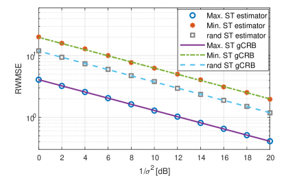
(a)

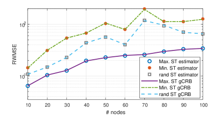
(b)

Figure 2: Linear Gaussian model with relative measurements: The graph CRB and the root WMSE for the three sensor allocation policies (Max. ST, Min. ST, and rand ST) for a) state estimation in power systems versus $\frac{1}{\sigma^{2}}$, in IEEE 118-bus system, $M=118$; and b) signals in random graphs versus the number of nodes in the network, for $\sigma^{2}=1$.

VII-B Bandlimited graph signal recovery

In this subsection we consider the problem of bandlimited graph signal recovery from Section VI for electrical networks, where ${\bf{w}}$ is zero-mean Gaussian noise with a known diagonal covariance matrix. The noise variance is set to $\sigma_{l}^{2}$ for the 64 buses (vertices) with loads and $\sigma_{g}^{2}=0.5\sigma_{l}^{2}$ for the 54 buses with generators. Thus, in this case ${\bf{J}}({\mbox{\boldmath$\theta$}})$ is a diagonal matrix with twos and fours on its diagonal, associated with load and generator buses, respectively. The signal, $\theta$, is set to the values in [45].

We assume a PSSE with direct access to a limited number of state (voltage) measurements. Thus, we assume the model in (53) for the special case where ${\bf{M}}$ is a sampling matrix associated with the subset of nodes ${\mathcal{S}}$, i.e. it satisfies ${\bf{M}}_{\mathcal{D},{\mathcal{S}}}={\bf{I}}_{{\mathcal{S}}}$ and ${\bf{M}}_{\mathcal{D},{\mathcal{S}}^{c}}={\bf{0}}$. This can be obtained in practical electrical networks by using Phasor Measurement Units (PMUs) [75]. However, installing PMUs on all possible buses is impossible due to budget constraints and limitations on power and communication resources. Thus, there is a need to establish a method to determine which information should be observed in the course of designing electrical networks. In power systems, the voltage signal, $\theta$, is shown to be smooth [12, 11]. However, the existing PSSE methods do not incorporate the smoothness and bandlimitedness constraints.

We compare the estimation performance of the CML estimator from (VI-D)-(68) and the proposed graph CRB from (60) for the following sensor selection policies:

1. Random sensor allocation policy (rand.) - named also uniform sampling [4], in which sample indices are chosen from ${1,\ldots,M}$ independently and randomly, where we bound the condition number of the matrix $(\bar{{\bf{Q}}}^{T}{\bf{V}}^{T}{\bf{M}}^{T}{\bf{M}}{\bf{V}}\bar{{\bf{Q}}})$ of the chosen set.

2. Minimum graph CRB (Alg. 1) - the sensor allocation policy from Algorithm 1.

3. Experimentally designed sampling (E-design) [76] - that maximizes the smallest singular value of the matrix ${\bf{M}}{\bf{V}}_{\mathcal{M},\mathcal{R}}={\bf{V}}_{{\mathcal{S}},\mathcal{R}}$.

4. A-optimal design (A-design) [32] - which is equivalent to minimizing the CCRB under i.i.d. Gaussian assumptions on the r.h.s. of (62).

The objective functions in 2)-4) lead to combinatorial problems, and, thus, are implemented here by greedy algorithms. In order to have a fair comparison, we implement all methods by Algorithm 1, where (4) is replaced by the chosen objective.

In Figs. 3.a and 3.b the root WMSE of the CML estimator from (VI-D)-(68) and the root of the graph CRB are presented for the IEEE 118-bus test case with the sampling policies 1)-4). In Fig. 3.a we present the results versus $\frac{M}{\sigma_{l}^{2}}$, where the cutoff frequency assumed by the graph CRB and by the estimator is set to $R=10$ and the number of sensors is $D=40$. The random sampling policy has been omitted from this figure since it has significantly high WMSE compared with the other methods. It can be seen that the proposed sampling allocation policy from Algorithm 1 has lower Dirichlet energy than that of the E-design [76] and A-design [32] methods, both in terms of the associated graph CRBs and the actual CML performance. For a low noise variance shown in the figure, i.e. low $\frac{1}{\sigma_{l}^{2}}$, the performance of the CML estimators deviated from the associated graph CRBs. This is due to the fact that in this figure we use real-data values of $\theta$, and, thus, $\theta$ is not a perfect bandlimited graph signal in practice. This mismatch prior assumption affects the performance, especially in the case of high SNRs. In Fig. 3.b we present the results versus the number of selected sensors for a perfectly $R=10$ bandlimited graph signal and for $\sigma_{l}^{2}=0.5$. It can be seen that the proposed sampling allocation policy from Algorithm 1, the A-design, and the E-design methods are all consistent, in the sense that the WMSE decreases with the number of samples, in contrast to the random sampling policy. The proposed method outperforms the other methods for any number of selected sensors. These figures demonstrate the fact that the sampling set of ${\bf{M}}$ affects the graph CRB differently for each choice of $D$ nodes. Therefore, by proper selection of sensors that are placed at the most informative locations (in the sense of the new gCRB), we can obtain the best performance for the same number of nodes, $R$.

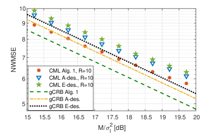
(a)

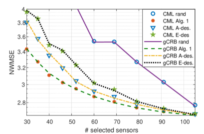
(b)

Figure 3: Bandlimited graph signal recovery: The graph CRB and the root WMSE for a random sensor allocation policy, and for Algorithm 1, A-design, and E-design methods for state estimation in power systems in IEEE 118-bus system (with $M=118$) for a) real-data values and assumed $R=10$ cutoff frequency and $D=40$ sensors versus $\frac{M}{\sigma_{l}^{2}}$; and b) $R=10$ bandlimited graph signal versus $D$ for $\sigma_{l}^{2}=0.5$.

In Figs. 4.a and 4.b the root WMSE of the CML estimator and the root of the graph CRB are presented for Erdős-R$\acute{\text{e}}$nyi graphs versus the number of nodes in the system, $M$, with the sampling policies 1)-4). We consider the case of $R=15$ graph frequencies and $D=0.2\times M$ sensors, and edge connecting probabilities $0.1$ and $0.05$. It can be seen that the proposed method outperforms the existing methods for any number of selected sensors and for the two edge connecting probabilities. The WMSE decreases as the network size decreases, as expected, since for all networks we have the same number of parameters to be estimated ($R$ parameters in the graph frequency domain), with an increasing number of sampled nodes, $D$. By comparing these figures, it can be seen that the estimation performance is better for less connected networks, i.e. the WMSE of all methods is lower for edge connecting probability of $p=0.05$.

In order to demonstrate the empirical complexity of Algorithm 1 for different network sizes and different graph topologies, the average computation time was evaluated by running Algorithm 1 using Matlab on an Intel Core(TM) i7-7600U CPU computer, 2.80 GHz. Fig. 4(c) shows the runtime of the different sampling policy methods versus $M$. The runtime of the proposed Algorithm 1 is identical to the runtime of the A-design method. The E-design method has a higher runtime than the others for small networks, but is more scalable to large networks. However, its estimation performance is worse than those of Algorithm 1 and E-design methods. It can be seen that for all methods, as more measurements are available, the computation time increases since the search is over more values. However, the edge connecting probability does not affect the runtime of the proposed approach.

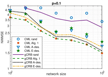
(a)

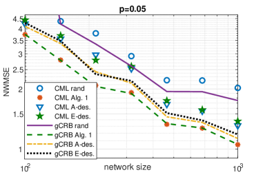
(b)

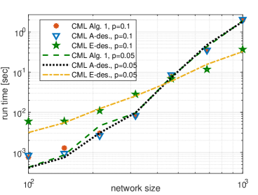
(c)

Figure 4: Bandlimited graph signal recovery: Performance of the random sensor allocation policy, and Algorithm 1, A-design, and E-design methods for Erdős-R$\acute{\text{e}}$nyi graphs with edge connecting probabilities of (a) $0.1$, (b) $0.05$, o and (c) both $0.1$ and $0.05$, with $R=15$-bandlimited signals and $D=0.2M$ sensors versus the number of nodes in terms of graph CRB and the root WMSE (a,b) and runtime (c).

VIII Conclusion

We consider the problem of graph signal recovery as a non-Bayesian parameter estimation under the Laplacian-based WMSE performance evaluation measure. We develop the graph CRB, which is a lower bound on the WMSE of any graph-unbiased estimator in the Lehmann sense. We present new sensor allocation policies that aim to reduce the graph CRB under a constrained amount of sensing nodes. The relation between the problem of finding the optimal sensor locations of relative measurements in the graph-CRB sense and the problem of finding the maximum weight spanning tree of a graph is demonstrated. The proposed graph CRB is evaluated and compared with the Laplacian-based WMSE of the CML estimator, for signal recovery over random graphs and for PSSE in electrical networks. Significant performance gains are observed from these simulations for using the optimal sensor locations. Thus, the proposed graph CRB can be used as a system design tool for sensing networks. Future work includes extensions to complex-valued systems and nonlinear examples, as well as developing low-complexity graph sampling methods based on the graph CRB that avoid SVD computation that are similar to the approaches in [70, 71]. In addition, methods that include the cost of communication and computation should be developed, in order to assess the performance of distributive algorithms for graph signal recovery.

Appendix A Derivation of (III-1)

By using the facts that $({\bf{V}}{\bf{\Lambda}}^{\frac{1}{2}})^{T}={\bf{\Lambda}}^{\frac{1}{2}}{\bf{V}}^{T}$ and that ${\bf{\Lambda}}^{\frac{1}{2}}$ is a diagonal matrix, the $(m,n)$th element of the matrix cost function ${\bf{C}}(\hat{{\mbox{\boldmath$\theta$}}},{\mbox{\boldmath$\theta$}})$, defined in (6), satisfies

$${\bf{C}}_{m,n}(\hat{{\mbox{\boldmath$\theta$}}},{\mbox{\boldmath$\theta$}})=\sum_{k=1}^{M}\sum_{l=1}^{M}[{\bf{\Lambda}}^{\frac{1}{2}}{\bf{V}}^{T}]_{m,k}[{\bf{\Lambda}}^{\frac{1}{2}}{\bf{V}}^{T}]_{n,l}\epsilon_{k}\epsilon_{l}\hskip 28.45274pt$$

$$={\bf{\Lambda}}^{\frac{1}{2}}_{m,m}{\bf{\Lambda}}^{\frac{1}{2}}_{n,n}\sum_{k=1}^{M}\sum_{l=1}^{M}{\bf{V}}_{k,m}{\bf{V}}_{l,n}\epsilon_{k}\epsilon_{l}\hskip 38.41139pt$$

$$=-\frac{1}{2}{\bf{\Lambda}}^{\frac{1}{2}}_{m,m}{\bf{\Lambda}}^{\frac{1}{2}}_{n,n}\sum_{k=1}^{M}\sum_{l=1}^{M}{\bf{V}}_{k,m}{\bf{V}}_{l,n}(\epsilon_{k}-\epsilon_{l})^{2}$$

$$+{\bf{\Lambda}}^{\frac{1}{2}}_{m,m}{\bf{\Lambda}}^{\frac{1}{2}}_{n,n}\sum_{k=1}^{M}{\bf{V}}_{k,m}\epsilon_{k}^{2}\times\sum_{l=1}^{M}{\bf{V}}_{l,n},\hskip 25.6073pt$$ (71)

where $\epsilon_{m}$, $m=1,\ldots,M$, are defined in (10). Since $(\lambda_{1},{\bf{v}}_{1})=(0,\frac{1}{\sqrt{M}}{\bf{1}})$ is the smallest eigenvalue-eigenvector pair of the positive semidefinite Laplacian matrix, then, ${\bf{1}}$ is orthogonal to the other $M-1$ eigenvectors of ${\bf{L}}$ that are given by the last $M-1$ columns of ${\bf{V}}$. Thus, $\sum\nolimits_{l=1}^{M}{\bf{V}}_{l,n}=0$, $\forall n=2,\ldots,M$. Since in addition ${\bf{\Lambda}}^{\frac{1}{2}}_{1,1}=0$, we can conclude that

$${\bf{\Lambda}}^{\frac{1}{2}}_{n,n}\sum\nolimits_{l=1}^{M}{\bf{V}}_{l,n}=0,~{}\forall n=1,\ldots,M.$$ (72)

By substituting (72) in (A), we obtain

$${\bf{C}}_{m,n}(\hat{{\mbox{\boldmath$\theta$}}},{\mbox{\boldmath$\theta$}})\hskip 142.26378pt$$

$$=-\frac{1}{2}{\bf{\Lambda}}^{\frac{1}{2}}_{m,m}{\bf{\Lambda}}^{\frac{1}{2}}_{n,n}\sum_{k=1}^{M}\sum_{l=1}^{M}{\bf{V}}_{k,m}{\bf{V}}_{l,n}(\epsilon_{k}-\epsilon_{l})^{2}.$$ (73)

By substituting

$$(\epsilon_{k}-\epsilon_{l})^{2}=(\epsilon_{k}-\epsilon_{m}+\epsilon_{m}-\epsilon_{l}+\epsilon_{n}-\epsilon_{n})^{2}\hskip 28.45274pt$$

$$=(\epsilon_{k}-\epsilon_{m})^{2}+(\epsilon_{l}-\epsilon_{n})^{2}+(\epsilon_{m}-\epsilon_{n})^{2}\hskip 19.91684pt$$

$$-2\left[(\epsilon_{k}-\epsilon_{m})(\epsilon_{l}-\epsilon_{n})\right.\hskip 91.04872pt$$

$$\left.+(\epsilon_{k}-\epsilon_{m})(\epsilon_{m}-\epsilon_{n})+(\epsilon_{l}-\epsilon_{n})(\epsilon_{m}-\epsilon_{n})\right]$$ (74)

into (A) and reordering the elements, we obtain

$${\bf{C}}_{m,n}(\hat{{\mbox{\boldmath$\theta$}}},{\mbox{\boldmath$\theta$}})={\bf{\Lambda}}^{\frac{1}{2}}_{m,m}{\bf{\Lambda}}^{\frac{1}{2}}_{n,n}\sum_{k=1}^{M}{\bf{V}}_{k,m}\sum_{l=1}^{M}{\bf{V}}_{l,n}\hskip 42.67912pt$$

$$\times\left\{-\frac{1}{2}\left[(\epsilon_{k}-\epsilon_{m})^{2}+(\epsilon_{l}-\epsilon_{n})^{2}+(\epsilon_{m}-\epsilon_{n})^{2}\right]\right.\hskip 9.95863pt$$

$$+\left[(\epsilon_{k}-\epsilon_{m})(\epsilon_{l}-\epsilon_{n})\right.\hskip 119.50148pt$$

$$\left.\left.+(\epsilon_{k}-\epsilon_{m})(\epsilon_{m}-\epsilon_{n})+(\epsilon_{l}-\epsilon_{n})(\epsilon_{m}-\epsilon_{n})\right]\right\}\hskip 22.76228pt$$

$$={\bf{\Lambda}}^{\frac{1}{2}}_{m,m}\sum_{k=1}^{M}{\bf{V}}_{k,m}\left[-\frac{1}{2}(\epsilon_{k}-\epsilon_{m})^{2}\right.\hskip 69.70915pt$$

$$\left.-\frac{1}{2}(\epsilon_{m}-\epsilon_{n})^{2}+(\epsilon_{k}-\epsilon_{m})(\epsilon_{m}-\epsilon_{n})\right]\hskip 48.36958pt$$

$$\times\left({\bf{\Lambda}}^{\frac{1}{2}}_{n,n}\sum_{l=1}^{M}{\bf{V}}_{l,n}\right)\hskip 125.19194pt$$

$$+{\bf{\Lambda}}^{\frac{1}{2}}_{n,n}\sum_{l=1}^{M}{\bf{V}}_{l,n}\left[-\frac{1}{2}(\epsilon_{l}-\epsilon_{n})^{2}+(\epsilon_{l}-\epsilon_{n})(\epsilon_{m}-\epsilon_{n})\right]$$

$$\times\left({\bf{\Lambda}}^{\frac{1}{2}}_{m,m}\sum_{k=1}^{M}{\bf{V}}_{k,m}\right)\hskip 118.07875pt$$

$$+{\bf{\Lambda}}^{\frac{1}{2}}_{m,m}{\bf{\Lambda}}^{\frac{1}{2}}_{n,n}\sum_{k=1}^{M}\sum_{l=1}^{M}{\bf{V}}_{k,m}{\bf{V}}_{l,n}(\epsilon_{k}-\epsilon_{m})(\epsilon_{l}-\epsilon_{n}).\hskip 6.82881pt$$ (75)

By substituting (72) in (A), we obtain the term in (III-1).

Appendix B Proof of Proposition 1

In this appendix, we prove that the graph-unbiasedness is obtained from the Lehmann unbiasedness definition in Definition 2 with the cost function from (6) and under the constrained set in (3). By substituting (6) in (18), we obtain that the Lehmann unbiasedness in this case requires that

$${\bf{\Lambda}}^{\frac{1}{2}}{\bf{V}}^{T}{\rm{E}}_{{\mbox{\boldmath{\scriptsize$\theta$}}}}\left[(\hat{{\mbox{\boldmath$\theta$}}}-{\mbox{\boldmath$\eta$}})(\hat{{\mbox{\boldmath$\theta$}}}-{\mbox{\boldmath$\eta$}})^{T}\right]{\bf{V}}{\bf{\Lambda}}^{\frac{1}{2}}\hskip 56.9055pt$$

$$\succeq{\bf{\Lambda}}^{\frac{1}{2}}{\bf{V}}^{T}{\rm{E}}_{{\mbox{\boldmath{\scriptsize$\theta$}}}}\left[(\hat{{\mbox{\boldmath$\theta$}}}-{\mbox{\boldmath$\theta$}})(\hat{{\mbox{\boldmath$\theta$}}}-{\mbox{\boldmath$\theta$}})^{T}\right]{\bf{V}}{\bf{\Lambda}}^{\frac{1}{2}},$$ (76)

$\forall{\mbox{\boldmath$\theta$}},{\mbox{\boldmath$\eta$}}\in\Omega_{\mbox{\boldmath{\scriptsize$\theta$}}}$. Similar to the derivation on p. 14 of [37], on adding and subtracting ${\rm{E}}_{{\mbox{\boldmath{\scriptsize$\theta$}}}}[\hat{{\mbox{\boldmath$\theta$}}}]$ inside the four round brackets in (B), this condition is reduced to

$${\bf{\Lambda}}^{\frac{1}{2}}{\bf{V}}^{T}{\rm{E}}_{{\mbox{\boldmath{\scriptsize$\theta$}}}}\left[({\rm{E}}_{{\mbox{\boldmath{\scriptsize$\theta$}}}}[\hat{{\mbox{\boldmath$\theta$}}}]-{\mbox{\boldmath$\eta$}})({\rm{E}}_{{\mbox{\boldmath{\scriptsize$\theta$}}}}[\hat{{\mbox{\boldmath$\theta$}}}]-{\mbox{\boldmath$\eta$}})^{T}\right]{\bf{V}}{\bf{\Lambda}}^{\frac{1}{2}}\hskip 42.67912pt$$

$$\succeq{\bf{\Lambda}}^{\frac{1}{2}}{\bf{V}}^{T}{\rm{E}}_{{\mbox{\boldmath{\scriptsize$\theta$}}}}\left[({\rm{E}}_{{\mbox{\boldmath{\scriptsize$\theta$}}}}[\hat{{\mbox{\boldmath$\theta$}}}]-{\mbox{\boldmath$\theta$}})({\rm{E}}_{{\mbox{\boldmath{\scriptsize$\theta$}}}}[\hat{{\mbox{\boldmath$\theta$}}}]-{\mbox{\boldmath$\theta$}})^{T}\right]{\bf{V}}{\bf{\Lambda}}^{\frac{1}{2}},$$ (77)

$\forall{\mbox{\boldmath$\theta$}},{\mbox{\boldmath$\eta$}}\in\Omega_{\mbox{\boldmath{\scriptsize$\theta$}}}$. By using the definition of the constrained set in (4), and since the range of ${\bf{U}}$ is the null-space of ${\bf{G}}$, it can be seen that for a given ${\mbox{\boldmath$\theta$}}\in\Omega_{\mbox{\boldmath{\scriptsize$\theta$}}}$, any ${\mbox{\boldmath$\eta$}}\in\Omega_{\mbox{\boldmath{\scriptsize$\theta$}}}$ can be written as (see, e.g. Section 4.2.4 in [77])

$${\mbox{\boldmath$\eta$}}={\mbox{\boldmath$\theta$}}+{\bf{U}}{\bf{w}},$$ (78)

for some vector ${\bf{w}}\in{\mathbb{R}}^{M-K}$. By substituting (78) in (B), we obtain

$${\bf{\Lambda}}^{\frac{1}{2}}{\bf{V}}^{T}{\rm{E}}_{{\mbox{\boldmath{\scriptsize$\theta$}}}}\left[({\rm{E}}_{{\mbox{\boldmath{\scriptsize$\theta$}}}}[\hat{{\mbox{\boldmath$\theta$}}}]-{\mbox{\boldmath$\theta$}}-{\bf{U}}{\bf{w}})({\rm{E}}_{{\mbox{\boldmath{\scriptsize$\theta$}}}}[\hat{{\mbox{\boldmath$\theta$}}}]-{\mbox{\boldmath$\theta$}}-{\bf{U}}{\bf{w}})^{T}\right]{\bf{V}}{\bf{\Lambda}}^{\frac{1}{2}}$$

$$\succeq{\bf{\Lambda}}^{\frac{1}{2}}{\bf{V}}^{T}{\rm{E}}_{{\mbox{\boldmath{\scriptsize$\theta$}}}}\left[({\rm{E}}_{{\mbox{\boldmath{\scriptsize$\theta$}}}}[\hat{{\mbox{\boldmath$\theta$}}}]-{\mbox{\boldmath$\theta$}})({\rm{E}}_{{\mbox{\boldmath{\scriptsize$\theta$}}}}[\hat{{\mbox{\boldmath$\theta$}}}]-{\mbox{\boldmath$\theta$}})^{T}\right]{\bf{V}}{\bf{\Lambda}}^{\frac{1}{2}},$$ (79)

$\forall{\mbox{\boldmath$\theta$}}\in\Omega_{\mbox{\boldmath{\scriptsize$\theta$}}},{\bf{w}}\in{\mathbb{R}}^{M-K}$. The condition in (B) can be rewritten as

$${\bf{\Lambda}}^{\frac{1}{2}}{\bf{V}}^{T}{\bf{U}}{\bf{w}}{\bf{w}}^{T}{\bf{U}}^{T}{\bf{V}}{\bf{\Lambda}}^{\frac{1}{2}}\succeq\hskip 120.92421pt$$

$${\bf{\Lambda}}^{\frac{1}{2}}{\bf{V}}^{T}\left(({\rm{E}}_{{\mbox{\boldmath{\scriptsize$\theta$}}}}[\hat{{\mbox{\boldmath$\theta$}}}]-{\mbox{\boldmath$\theta$}}){\bf{w}}^{T}{\bf{U}}^{T}+{\bf{U}}{\bf{w}}({\rm{E}}_{{\mbox{\boldmath{\scriptsize$\theta$}}}}[\hat{{\mbox{\boldmath$\theta$}}}]-{\mbox{\boldmath$\theta$}})^{T}\right){\bf{V}}{\bf{\Lambda}}^{\frac{1}{2}}.$$ (80)

A necessary condition for (B) to be satisfied is that

$${\bf{w}}^{T}{\bf{U}}^{T}{\bf{L}}{\bf{U}}{\bf{w}}\geq 2{\bf{w}}^{T}{\bf{U}}^{T}{\bf{L}}({\rm{E}}_{{\mbox{\boldmath{\scriptsize$\theta$}}}}[\hat{{\mbox{\boldmath$\theta$}}}]-{\mbox{\boldmath$\theta$}}),$$ (81)

where we applied the trace operator on both sides on (B) and used the trace operator properties. Since the l.h.s. of (81) is nonnegative, (19) is a sufficient condition for (81) to hold. In addition, since the condition in (81) should be satisfied for any ${\bf{w}}\in{\mathbb{R}}^{M-K}$, it should be satisfied in particular for both ${\bf{w}}=\epsilon{\bf{e}}_{k}\in{\mathbb{R}}^{M-K}$ and ${\bf{w}}=-\epsilon{\bf{e}}_{k}\in{\mathbb{R}}^{M-K}$, $k=1,\ldots,K$, with small positive $\epsilon$. By substituting these values in (81), we require

$$\epsilon^{2}{\bf{e}}_{k}^{T}{\bf{U}}^{T}{\bf{L}}{\bf{U}}{\bf{e}}_{k}\geq\pm\epsilon 2{\bf{e}}_{k}^{T}{\bf{U}}^{T}{\bf{L}}({\rm{E}}_{{\mbox{\boldmath{\scriptsize$\theta$}}}}[\hat{{\mbox{\boldmath$\theta$}}}]-{\mbox{\boldmath$\theta$}}),$$ (82)

for any $k=1,\ldots,K$, which, by taking the limit $\epsilon\rightarrow 0^{+}$, implies that $[{\bf{U}}^{T}{\bf{L}}({\rm{E}}_{{\mbox{\boldmath{\scriptsize$\theta$}}}}[\hat{{\mbox{\boldmath$\theta$}}}]-{\mbox{\boldmath$\theta$}})]_{k}=0$ for any $k=1,\ldots,K$, and, thus, (19) is also a necessary condition for (81) to be satisfied. Thus, we can conclude that (19) is a sufficient condition for the graph unbiasedness of estimators in the Lehmann sense in (B).

Appendix C Proof of Theorem 1

The following proof for the development of the graph CRB is along the path of the development of the CCRB on the MSE in a conventional estimation problem in [42]. Let ${\bf{W}}\in{\mathbb{R}}^{M\times M}$ be an arbitrary matrix. Then, the Cauchy-Schwarz inequality implies that

$${\bf{\Lambda}}^{\frac{1}{2}}{\bf{V}}^{T}{\rm{E}}_{\mbox{\boldmath{\scriptsize$\theta$}}}\left[\left(\hat{{\mbox{\boldmath$\theta$}}}-{\mbox{\boldmath$\theta$}}-{\bf{W}}{\bf{U}}{\bf{U}}^{T}\nabla_{{\mbox{\boldmath{\scriptsize$\theta$}}}}^{T}\log f({\bf{x}};{\mbox{\boldmath$\theta$}})\right)\right.\hskip 35.56593pt$$

$$\times\left.\left(\hat{{\mbox{\boldmath$\theta$}}}-{\mbox{\boldmath$\theta$}}-{\bf{W}}{\bf{U}}{\bf{U}}^{T}\nabla_{{\mbox{\boldmath{\scriptsize$\theta$}}}}^{T}\log f({\bf{x}};{\mbox{\boldmath$\theta$}})\right)^{T}\right]{\bf{V}}{\bf{\Lambda}}^{\frac{1}{2}}\succeq{\bf{0}}.$$ (83)

Under Condition C.2, the matrix inequality in (C) implies that

$${\bf{\Lambda}}^{\frac{1}{2}}{\bf{V}}^{T}{\rm{E}}_{\mbox{\boldmath{\scriptsize$\theta$}}}[(\hat{{\mbox{\boldmath$\theta$}}}-{\mbox{\boldmath$\theta$}})(\hat{{\mbox{\boldmath$\theta$}}}-{\mbox{\boldmath$\theta$}})^{T}]{\bf{V}}{\bf{\Lambda}}^{\frac{1}{2}}\hskip 91.04872pt$$

$$\succeq{\bf{\Lambda}}^{\frac{1}{2}}{\bf{V}}^{T}{\rm{E}}_{\mbox{\boldmath{\scriptsize$\theta$}}}[(\hat{{\mbox{\boldmath$\theta$}}}-{\mbox{\boldmath$\theta$}})\nabla_{{\mbox{\boldmath{\scriptsize$\theta$}}}}\log f({\bf{x}};{\mbox{\boldmath$\theta$}})]{\bf{U}}{\bf{U}}^{T}{\bf{W}}^{T}{\bf{V}}{\bf{\Lambda}}^{\frac{1}{2}}\hskip 5.69046pt$$

$$+{\bf{\Lambda}}^{\frac{1}{2}}{\bf{V}}^{T}{\bf{W}}{\bf{U}}{\bf{U}}^{T}{\rm{E}}_{\mbox{\boldmath{\scriptsize$\theta$}}}[\nabla_{{\mbox{\boldmath{\scriptsize$\theta$}}}}^{T}\log f({\bf{x}};{\mbox{\boldmath$\theta$}})(\hat{{\mbox{\boldmath$\theta$}}}-{\mbox{\boldmath$\theta$}})^{T}]{\bf{V}}{\bf{\Lambda}}^{\frac{1}{2}}$$

$$-{\bf{\Lambda}}^{\frac{1}{2}}{\bf{V}}^{T}{\bf{W}}{\bf{U}}{\bf{U}}^{T}{\bf{J}}({\mbox{\boldmath$\theta$}}){\bf{U}}{\bf{U}}^{T}{\bf{W}}^{T}{\bf{V}}{\bf{\Lambda}}^{\frac{1}{2}}.\hskip 46.23572pt$$ (84)

By using regularity condition C.1 with $g({\bf{x}},{\mbox{\boldmath$\theta$}})=(\hat{{\mbox{\boldmath$\theta$}}}-{\mbox{\boldmath$\theta$}})f({\bf{x}};{\mbox{\boldmath$\theta$}})$ and the product rule, it can be verified that (see, e.g. Appendix 3B in [52])

$${\rm{E}}_{\mbox{\boldmath{\scriptsize$\theta$}}}\left[(\hat{{\mbox{\boldmath$\theta$}}}-{\mbox{\boldmath$\theta$}})\nabla_{{\mbox{\boldmath{\scriptsize$\theta$}}}}\log f({\bf{x}};{\mbox{\boldmath$\theta$}})\right]={\bf{I}}_{M}+\nabla_{{\mbox{\boldmath{\scriptsize$\theta$}}}}{\rm{E}}_{\mbox{\boldmath{\scriptsize$\theta$}}}[\hat{{\mbox{\boldmath$\theta$}}}-{\mbox{\boldmath$\theta$}}].$$ (85)

Thus, by multiplying (85) by ${\bf{L}}$ and ${\bf{U}}$ from left and right, respectively, and substituting the local graph-unbiasedness from (22) in Definition 3, we obtain

$${\bf{L}}{\rm{E}}_{\mbox{\boldmath{\scriptsize$\theta$}}}\left[(\hat{{\mbox{\boldmath$\theta$}}}-{\mbox{\boldmath$\theta$}})\nabla_{{\mbox{\boldmath{\scriptsize$\theta$}}}}\log f({\bf{x}};{\mbox{\boldmath$\theta$}})\right]{\bf{U}}={\bf{L}}{\bf{U}}.$$ (86)

Or, equivalently, by using ${\bf{L}}={\bf{V}}{\bf{\Lambda}}{\bf{V}}^{T}$ and the fact that ${\bf{\Lambda}}$ is a nonnegative diagonal matrix,

$${\bf{\Lambda}}^{\frac{1}{2}}{\bf{V}}^{T}{\rm{E}}_{\mbox{\boldmath{\scriptsize$\theta$}}}\left[(\hat{{\mbox{\boldmath$\theta$}}}-{\mbox{\boldmath$\theta$}})\nabla_{{\mbox{\boldmath{\scriptsize$\theta$}}}}\log f({\bf{x}};{\mbox{\boldmath$\theta$}})\right]{\bf{U}}={\bf{\Lambda}}^{\frac{1}{2}}{\bf{V}}^{T}{\bf{U}}.$$ (87)

By substituting (7) and (87) in (C), we obtain

$${\rm{E}}_{{\mbox{\boldmath{\scriptsize$\theta$}}}}[{\bf{C}}(\hat{{\mbox{\boldmath$\theta$}}},{\mbox{\boldmath$\theta$}})]\succeq{\bf{\Lambda}}^{\frac{1}{2}}{\bf{V}}^{T}{\bf{U}}{\bf{U}}^{T}{\bf{W}}^{T}{\bf{V}}{\bf{\Lambda}}^{\frac{1}{2}}\hskip 64.01869pt$$

$$+{\bf{\Lambda}}^{\frac{1}{2}}{\bf{V}}^{T}{\bf{W}}{\bf{U}}{\bf{U}}^{T}{\bf{V}}{\bf{\Lambda}}^{\frac{1}{2}}\hskip 64.01869pt$$

$$-{\bf{\Lambda}}^{\frac{1}{2}}{\bf{V}}^{T}{\bf{W}}{\bf{U}}{\bf{U}}^{T}{\bf{J}}({\mbox{\boldmath$\theta$}}){\bf{U}}{\bf{U}}^{T}{\bf{W}}^{T}{\bf{V}}{\bf{\Lambda}}^{\frac{1}{2}}.$$ (88)

Now, let ${\bf{W}}$ be such that

$${\bf{W}}{\bf{U}}={\bf{U}}\left({\bf{U}}^{T}{\bf{J}}({\mbox{\boldmath$\theta$}}){\bf{U}}\right)^{\dagger}.$$ (89)

By substituting (89) in (C) and using ${\bf{A}}^{\dagger}{\bf{A}}{\bf{A}}^{\dagger}={\bf{A}}^{\dagger}$ for any matrix ${\bf{A}}$, we obtain the bound in (25)-(26).

According to the conditions for equality in the Cauchy-Schwarz inequality, for any given matrix ${\bf{W}}$, the equality holds in (C) iff

$${\bf{\Lambda}}^{\frac{1}{2}}{\bf{V}}^{T}(\hat{{\mbox{\boldmath$\theta$}}}-{\mbox{\boldmath$\theta$}})=\zeta({\mbox{\boldmath$\theta$}}){\bf{\Lambda}}^{\frac{1}{2}}{\bf{V}}^{T}{\bf{W}}{\bf{U}}{\bf{U}}^{T}\nabla_{{\mbox{\boldmath{\scriptsize$\theta$}}}}^{T}\log f({\bf{x}};{\mbox{\boldmath$\theta$}}),$$ (90)

where $\zeta({\mbox{\boldmath$\theta$}})$ is a scalar function of $\theta$. By substituting (89) in (90), we obtain the following condition for achievability:

$${\bf{\Lambda}}^{\frac{1}{2}}{\bf{V}}^{T}(\hat{{\mbox{\boldmath$\theta$}}}-{\mbox{\boldmath$\theta$}})=\hskip 128.0374pt$$

$$\zeta({\mbox{\boldmath$\theta$}}){\bf{\Lambda}}^{\frac{1}{2}}{\bf{V}}^{T}{\bf{U}}\left({\bf{U}}^{T}{\bf{J}}({\mbox{\boldmath$\theta$}}){\bf{U}}\right)^{\dagger}{\bf{U}}^{T}\nabla_{{\mbox{\boldmath{\scriptsize$\theta$}}}}^{T}\log f({\bf{x}};{\mbox{\boldmath$\theta$}}).$$ (91)

Computing the expected quadratic term (${\bf{a}}{\bf{a}}^{T}$) of each side of (C), substituting (7) and (24), we obtain

$${\rm{E}}_{{\mbox{\boldmath{\scriptsize$\theta$}}}}[{\bf{C}}(\hat{{\mbox{\boldmath$\theta$}}},{\mbox{\boldmath$\theta$}})]=\zeta^{2}({\mbox{\boldmath$\theta$}}){\bf{B}}({\mbox{\boldmath$\theta$}}),$$ (92)

where ${\bf{B}}({\mbox{\boldmath$\theta$}})$ is defined in (26). Thus, for obtaining equality in (25), we require $\zeta({\mbox{\boldmath$\theta$}})=\pm 1$. It can be verified that in order for $\hat{{\mbox{\boldmath$\theta$}}}$ from (92) to satisfy (22) from Definition 3, we must take $\zeta({\mbox{\boldmath$\theta$}})=1$. By substituting $\zeta({\mbox{\boldmath$\theta$}})=1$ in (C), we obtain (27).

Appendix D Derivation of (43)

Since $\bar{{\bf{E}}}\bar{{\bf{E}}}^{T}$ is a Laplacian matrix, it satisfies ${\bf{1}}^{T}\left(\bar{{\bf{E}}}\bar{{\bf{E}}}^{T}-\frac{1}{M}{\bf{1}}{\bf{1}}^{T}\right)^{-1}=-{\bf{1}}^{T}$ and $\left(\bar{{\bf{E}}}\bar{{\bf{E}}}^{T}-\frac{1}{M}{\bf{1}}{\bf{1}}^{T}\right)^{-1}{\bf{1}}=-{\bf{1}}$. By using these results, the null-space property of ${\bf{L}}$, and $\bar{{\bf{L}}}=\bar{{\bf{L}}}-\frac{1}{M}{\bf{1}}{\bf{1}}^{T}+\frac{1}{M}{\bf{1}}{\bf{1}}^{T}$, we obtain that (42) can be rewritten as

$${\bf{J}}({\mbox{\boldmath$\theta$}})=\frac{1}{\sigma^{2}}\hskip 170.71652pt$$

$$\times\left(\bar{{\bf{L}}}-\frac{1}{M}{\bf{1}}{\bf{1}}^{T}\right)\left(\bar{{\bf{E}}}\bar{{\bf{E}}}^{T}-\frac{1}{M}{\bf{1}}{\bf{1}}^{T}\right)^{-1}\left(\bar{{\bf{L}}}-\frac{1}{M}{\bf{1}}{\bf{1}}^{T}\right).$$ (93)

By using Lemma 3 from [78], we obtain

$${\bf{J}}^{\dagger}({\mbox{\boldmath$\theta$}})=\sigma^{2}({\bf{I}}-\frac{{\mbox{\boldmath$\psi$}}{\mbox{\boldmath$\psi$}}^{T}}{{\mbox{\boldmath$\psi$}}^{T}{\mbox{\boldmath$\psi$}}})\left(\bar{{\bf{L}}}-\frac{1}{M}{\bf{1}}{\bf{1}}^{T}\right)^{-1}\hskip 42.67912pt$$

$$\times\left(\bar{{\bf{E}}}\bar{{\bf{E}}}^{T}-\frac{1}{M}{\bf{1}}{\bf{1}}^{T}\right)\left(\bar{{\bf{L}}}-\frac{1}{M}{\bf{1}}{\bf{1}}^{T}\right)^{-1}\left({\bf{I}}-\frac{{\bf{y}}{\bf{y}}^{T}}{{\bf{y}}^{T}{\bf{y}}}\right),$$ (94)

where ${\mbox{\boldmath$\psi$}}=-\frac{1}{\sqrt{M}}{\bf{1}}$ ${\bf{y}}^{T}=\frac{1}{\sqrt{M}}{\bf{1}}^{T}$, and we used the facts that ${\bf{1}}^{T}\left(\bar{{\bf{E}}}\bar{{\bf{E}}}^{T}-\frac{1}{M}{\bf{1}}{\bf{1}}^{T}\right)^{-1}=-{\bf{1}}^{T}$ and $\left(\bar{{\bf{E}}}\bar{{\bf{E}}}^{T}-\frac{1}{M}{\bf{1}}{\bf{1}}^{T}\right)^{-1}{\bf{1}}=-{\bf{1}}$. By substituting $\psi$ and ${\bf{y}}$ in (D), one obtains

$${\bf{J}}^{\dagger}({\mbox{\boldmath$\theta$}})=\sigma^{2}({\bf{I}}-\frac{1}{M}{\bf{1}}{\bf{1}}^{T})\left(\bar{{\bf{L}}}-\frac{1}{M}{\bf{1}}{\bf{1}}^{T}\right)^{-1}\hskip 28.45274pt$$

$$\times\left(\bar{{\bf{E}}}\bar{{\bf{E}}}^{T}-\frac{1}{M}{\bf{1}}{\bf{1}}^{T}\right)\left(\bar{{\bf{L}}}-\frac{1}{M}{\bf{1}}{\bf{1}}^{T}\right)^{-1}({\bf{I}}-\frac{1}{M}{\bf{1}}{\bf{1}}^{T}).$$ (95)

It is well known that the pseudo-inverse of a Laplacian matrix with $M$ nodes is given by [56]

$$\bar{{\bf{L}}}^{\dagger}=\left(\bar{{\bf{L}}}-\frac{1}{M}{\bf{1}}{\bf{1}}^{T}\right)^{-1}+\frac{1}{M}{\bf{1}}{\bf{1}}^{T}.$$ (96)

By substituting (96) in (D) and using the null-space property of $\bar{{\bf{E}}}\bar{{\bf{E}}}^{T}$ and $\bar{{\bf{L}}}^{\dagger}$, we obtain (43).

References

- [1] M. Newman, Networks: An Introduction, Oxford University Press, Inc., New York, NY, USA, 2010.
- [2] D. I. Shuman, S. K. Narang, P. Frossard, A. Ortega, and P. Vandergheynst, “The emerging field of signal processing on graphs: Extending high-dimensional data analysis to networks and other irregular domains,” IEEE Signal Processing Magazine, vol. 30, no. 3, pp. 83–98, May 2013.
- [3] A. Sandryhaila and J. M. F. Moura, “Discrete signal processing on graphs,” IEEE Trans. Signal Processing, vol. 61, no. 7, pp. 1644–1656, Apr. 2013.
- [4] S. Chen, R. Varma, A. Singh, and J. Kovačević, “Signal recovery on graphs: Fundamental limits of sampling strategies,” IEEE Trans. Signal and Information Processing over Networks, vol. 2, no. 4, pp. 539–554, Dec. 2016.
- [5] A. Ortega, P. Frossard, J. Kovačević, J. M. F. Moura, and P. Vandergheynst, “Graph signal processing: Overview, challenges, and applications,” Proceedings of the IEEE, vol. 106, no. 5, pp. 808–828, May 2018.
- [6] S. Segarra, S. P. Chepuri, A. G. Marques, and G. Leus, “Statistical graph signal processing: Stationarity and spectral estimation,” in Cooperative and Graph Signal Processing, pp. 325–347. Elsevier, 2018.
- [7] A. G. Marques, S. Segarra, G. Leus, and A. Ribeiro, “Sampling of graph signals with successive local aggregations,” IEEE Trans. Signal Processing, vol. 64, no. 7, pp. 1832–1843, 2016.
- [8] A. Singer and Y. Shkolnisky, “Three-dimensional structure determination from common lines in cryo-EM by eigenvectors and semidefinite programming,” SIAM journal on imaging sciences, vol. 4, no. 2, pp. 543–572, 2011.
- [9] A. Giridhar and P. R. Kumar, “Distributed clock synchronization over wireless networks: Algorithms and analysis,” in IEEE Conference on Decision and Control (CDC), Dec. 2006, pp. 4915–4920.
- [10] G. B. Giannakis, V. Kekatos, N. Gatsis, S. Kim, H. Zhu, and B. F. Wollenberg, “Monitoring and optimization for power grids: A signal processing perspective,” IEEE Signal Processing Magazine, vol. 30, no. 5, pp. 107–128, Sept. 2013.
- [11] E. Drayer and T. Routtenberg, “Detection of false data injection attacks in smart grids based on graph signal processing,” IEEE Systems Journal, vol. 14, no. 2, pp. 1886–1896, June 2020, doi: 10.1109/JSYST.2019.2927469.
- [12] E. Drayer and T. Routtenberg, “Detection of false data injection attacks in power systems with graph fourier transform,” in GlobalSIP, Nov. 2018, pp. 890–894.
- [13] S. Grotas, Y. Yakoby, I. Gera, and T. Routtenberg, “Power systems topology and state estimation by graph blind source separation,” IEEE Trans. Signal Processing, vol. 67, no. 8, pp. 2036–2051, Apr. 2019.
- [14] Z. Wang and A. C. Bovik, “Mean squared error: Love it or leave it? a new look at signal fidelity measures,” IEEE signal processing magazine, vol. 26, no. 1, pp. 98–117, 2009.
- [15] J. Jia, M. T. Schaub, S. Segarra, and A. R. Benson, “Graph-based semi-supervised and active learning for edge flows,” in International Conference on Knowledge Discovery and Data Mining, 2019, p. 761–771.
- [16] A. Breloy, G. Ginolhac, A. Renaux, and F. Bouchard, “Intrinsic Cramr-Rao bounds for scatter and shape matrices estimation in CES distributions,” IEEE Signal Processing Letters, vol. 26, no. 2, pp. 262–266, Feb. 2019.
- [17] T. Routtenberg and J. Tabrikian, “Non-Bayesian periodic Cramr-Rao bound,” IEEE Trans. Signal Processing, vol. 61, no. 4, pp. 1019–1032, Feb. 2013.
- [18] A. Sandryhaila and J. M. F. Moura, “Big data analysis with signal processing on graphs: Representation and processing of massive data sets with irregular structure,” IEEE Signal Processing Magazine, vol. 31, no. 5, pp. 80–90, Sept. 2014.
- [19] F. Nielsen, “Cramér-rao lower bound and information geometry,” in Connected at Infinity II, pp. 18–37. Springer, 2013.
- [20] P. Barooah and J. P. Hespanha, “Estimation on graphs from relative measurements,” IEEE Control Systems Magazine, vol. 27, no. 4, pp. 57–74, Aug 2007.
- [21] P. Barooah and J. P. Hespanha, “Estimation from relative measurements: Electrical analogy and large graphs,” IEEE Trans. Signal Processing, vol. 56, no. 6, pp. 2181–2193, 2008.
- [22] A. Abur and A. Gomez-Exposito, Power System State Estimation: Theory and Implementation, Marcel Dekker, 2004.
- [23] A. Kroizer, Y. C. Eldar, and T. Routtenberg, “Modeling and recovery of graph signals and difference-based signals,” in GlobalSIP, Nov. 2019, pp. 1–5.
- [24] M. Zheng, J. Bu, C. Chen, C. Wang, L. Zhang, G. Qiu, and D. Cai, “Graph regularized sparse coding for image representation,” IEEE Trans. Image Processing, vol. 20, no. 5, pp. 1327–1336, May 2011.
- [25] A. Elmoataz, O. Lezoray, and S. Bougleux, “Nonlocal discrete regularization on weighted graphs: A framework for image and manifold processing,” IEEE Trans. Image Processing, vol. 17, no. 7, pp. 1047–1060, July 2008.
- [26] D. Cai, X. He, J. Han, and T. S. Huang, “Graph regularized nonnegative matrix factorization for data representation,” IEEE Trans. pattern analysis and machine intelligence, vol. 33, no. 8, pp. 1548–1560, 2010.
- [27] N. Shahid, V. Kalofolias, X. Bresson, M. Bronstein, and P. Vandergheynst, “Robust principal component analysis on graphs,” in IEEE International Conference on Computer Vision, 2015, pp. 2812–2820.
- [28] F. Wang and C. Zhang, “Label propagation through linear neighborhoods,” IEEE Trans. Knowledge and Data Engineering, vol. 20, no. 1, pp. 55–67, 2007.
- [29] M. Belkin, I. Matveeva, and P. Niyogi, “Regularization and semi-supervised learning on large graphs,” in International Conference on Computational Learning Theory. Springer, 2004, pp. 624–638.
- [30] O. Chapelle, B. Scholkopf, and A. Zien, Semi-Supervised Learning, Cambridge, Massachusetts: The MIT Press, 2006.
- [31] D. I. Shuman, B. Ricaud, and P. Vandergheynst, “A windowed graph Fourier transform,” in IEEE Statistical Signal Processing Workshop (SSP), Aug. 2012, pp. 133–136.
- [32] A. Anis, A. Gadde, and Antonio A. Ortega, “Efficient sampling set selection for bandlimited graph signals using graph spectral proxies,” IEEE Trans. Signal Processing, vol. 64, no. 14, pp. 3775–3789, 2016.
- [33] N. Boumal, “On intrinsic Cramr-Rao bounds for Riemannian submanifolds and quotient manifolds,” IEEE Trans. Signal Processing, vol. 61, no. 7, pp. 1809–1821, Apr. 2013.
- [34] N. Boumal, A. Singer, P. A. Absil, and V. D. Blondel, “Cramr-Rao bounds for synchronization of rotations,” Information and Inference: A Journal of the IMA, vol. 3, no. 1, pp. 1–39, 2014.
- [35] S. Rosenberg, The Laplacian on a Riemannian manifold: an introduction to analysis on manifolds, Number 31. Cambridge University Press, 1997.
- [36] L. I. Rudin, S. Osher, and E. Fatemi, “Nonlinear total variation based noise removal algorithms,” Physica D: nonlinear phenomena, vol. 60, no. 1-4, pp. 259–268, 1992.
- [37] E. L. Lehmann and J. P. Romano, Testing Statistical Hypotheses, Springer Texts in Statistics, New York, 3 edition, 2005.
- [38] A. Deshpande, C. Guestrin, S.R. Madden, J. M. Hellerstein, and W. Hong, “Model-driven data acquisition in sensor networks,” in international conference on Very large data bases, 2004, pp. 588–599.
- [39] A. Wiesel and A. O. Hero, “Distributed covariance estimation in Gaussian graphical models,” IEEE Trans. Signal Processing, vol. 60, no. 1, pp. 211–220, Jan 2012.
- [40] S. Bezuglyi and P. E. Jorgensen, “Graph Laplace and Markov operators on a measure space,” in Linear Systems, Signal Processing and Hypercomplex Analysis, pp. 67–138. Springer, 2019.
- [41] J. D. Gorman and A. O. Hero, “Lower bounds for parametric estimation with constraints,” IEEE Trans. Inf. Theory, vol. 36, no. 6, pp. 1285–1301, Nov. 1990.
- [42] P. Stoica and B. C. Ng, “On the Cramr-Rao bound under parametric constraints,” IEEE Signal Process. Lett., vol. 5, no. 7, pp. 177–179, July 1998.
- [43] E. Nitzan, T. Routtenberg, and J. Tabrikian, “Cramr-Rao bound for constrained parameter estimation using Lehmann-unbiasedness,” IEEE Trans. Signal Processing, vol. 67, no. 3, pp. 753–768, Feb. 2019.
- [44] Z. Ben-Haim and Y. C. Eldar, “The Cramr-Rao bound for estimating a sparse parameter vector,” IEEE Trans. Signal Process., vol. 58, no. 6, pp. 3384–3389, June 2010.
- [45] “Power systems test case archive,” Tech. Rep., University of Washington, http://www.ee.washington.edu/research/pstca/.
- [46] Y. C. Eldar, “Universal weighted MSE improvement of the least-squares estimator,” IEEE Trans. Signal Process., vol. 56, no. 5, pp. 1788–1800, May 2008.
- [47] M. Belkin and P. Niyogi, “Laplacian eigenmaps and spectral techniques for embedding and clustering,” in Advances in neural information processing systems, 2002, pp. 585–591.
- [48] T. Routtenberg and L. Tong, “Estimation after parameter selection: Performance analysis and estimation methods,” IEEE Trans. Signal Processing, vol. 64, no. 20, pp. 5268–5281, Oct. 2016.
- [49] T. Routtenberg, Parameter Estimation under Arbitrary Cost Functions with Constraints, Ph.D. thesis, http://aranne5.bgu.ac.il/others/RouttenbergTirza3.pdf, Ben-Gurion University of the Negev, May 2012.
- [50] P. Stoica and T. L. Marzetta, “Parameter estimation problems with singular information matrices,” IEEE Trans. Signal Processing, vol. 49, no. 1, pp. 87–90, 2001.
- [51] T. J. Moore, B. M. Sadler, and R. J. Kozick, “Maximum-likelihood estimation, the Cramr-Rao bound, and the method of scoring with parameter constraints,” IEEE Trans. Signal Process., vol. 56, no. 3, pp. 895–908, Mar. 2008.
- [52] S. M. Kay, Fundamentals of statistical signal processing: Estimation Theory, vol. 1, Prentice Hall PTR, Englewood Cliffs (N.J.), 1993.
- [53] S. D. Howard, D. Cochran, W. Moran, and F. R. Cohen, “Estimation and registration on graphs,” arXiv, 1010.2983, 2010.
- [54] S. Prabhu and I. Pe’er, “Ultrafast genome-wide scan for SNP–SNP interactions in common complex disease,” Genome research, vol. 22, no. 11, pp. 2230–2240, 2012.
- [55] K. S. Lu and A. Ortega, “Closed form solutions of combinatorial graph Laplacian estimation under acyclic topology constraints,” arXiv preprint arXiv:1711.00213, 2017.
- [56] I. Gutman and W. Xiao, “Generalized inverse of the Laplacian matrix and some applications,” Bulletin, , no. 29, pp. 15–23, 2004.
- [57] S. Narasimhan and C. Jordache, Data Reconciliation and Gross Error Detection: An Intelligent Use of Process Data, Elsevier Science, 1999.
- [58] D. A. Spielman and J. Woo, “A note on preconditioning by low-stretch spanning trees,” arXiv preprint arXiv:0903.2816, 2009.
- [59] N. Alon, R. M. Karp, D. Peleg, and D. West, “A graph-theoretic game and its application to the k-server problem,” SIAM Journal on Computing, vol. 24, no. 1, pp. 78–100, 1995.
- [60] M. B. Cohen, G. L. Miller, J. W. Pachocki, R. Peng, and S. C. Xu, “Stretching stretch,” arXiv preprint arXiv:1401.2454, 2014.
- [61] D. Jungnickel, Graphs, networks and algorithms, vol. 5, Springer Science & Business Media, 2007.
- [62] P. A. Papp, S. Kisfaludi-Bak, and Z. Kiraly, Low-stretch spanning trees, Ph.D. thesis, Eotvos Lorand University, 2014.
- [63] I. Abraham, Y. Bartal, and O. Neiman, “Nearly tight low stretch spanning trees,” in IEEE Symposium on Foundations of Computer Science, 2008, pp. 781–790.
- [64] S. Chen, A. Sandryhaila, J. M. F. Moura, and J. Kovačević, “Signal recovery on graphs: Variation minimization,” IEEE Trans. Signal Processing, vol. 63, no. 17, pp. 4609–4624, Sept 2015.
- [65] F. Gama, E. Isufi, A. Ribeiro, and G. Leus, “Controllability of bandlimited graph processes over random time varying graphs,” IEEE Trans. Signal Processing, vol. 67, no. 24, pp. 6440–6454, 2019.
- [66] Y. Yankelevsky and M. Elad, “Dual graph regularized dictionary learning,” IEEE Trans. Signal and Information Processing over Networks, vol. 2, no. 4, pp. 611–624, Dec. 2016.
- [67] E. Bayram, D. Thanou, E. Vural, and P. Frossard, “Mask combination of multi-layer graphs for global structure inference,” IEEE Trans. Signal and Information Processing over Networks, vol. 6, pp. 394–406, 2020.
- [68] Xianghui Mao and Yuantao Gu, Time-Varying Graph Signals Reconstruction, pp. 293–316, Springer International Publishing, Cham, 2019.
- [69] A. Sakiyama, Y. Tanaka, T. Tanaka, and A. Ortega, “Eigendecomposition-free sampling set selection for graph signals,” IEEE Trans. Signal Processing, vol. 67, no. 10, pp. 2679–2692, 2019.
- [70] F. Wang, G. Cheung, and Y. Wang, “Low-complexity graph sampling with noise and signal reconstruction via Neumann series,” IEEE Trans. Signal Processing, vol. 67, no. 21, pp. 5511–5526, 2019.
- [71] Y. Bai, F. Wang, G. Cheung, Y. Nakatsukasa, and W. Gao, “Fast graph sampling set selection using Gershgorin disc alignment,” IEEE Trans. Signal Processing, vol. 68, pp. 2419–2434, 2020.
- [72] G. Ortiz-Jiménez, M. Coutino, S. P. Chepuri, and G. Leus, “Sparse sampling for inverse problems with tensors,” IEEE Trans. Signal Processing, vol. 67, no. 12, pp. 3272–3286, 2019.
- [73] Y. Zhao, J. Chen, A. Goldsmith, and H. V. Poor, “Identification of outages in power systems with uncertain states and optimal sensor locations,” IEEE Journal of Selected Topics in Signal Processing, vol. 8, no. 6, pp. 1140–1153, 2014.
- [74] D. J. Watts and S. H. Strogatz, “Collective dynamics of small-world networks,” Nature, pp. 393–440, 1998.
- [75] A.G. Phadke and J.S. Thorp, Synchronized Phasor Measurements and Their Applications, New York: Springer Science, 2008.
- [76] S. Chen, R. Varma, A. Sandryhaila, and J. Kovačević, “Discrete signal processing on graphs: Sampling theory,” IEEE Trans. Signal Processing, vol. 63, no. 24, pp. 6510–6523, 2015.
- [77] S. Boyd and L. Vandenberghe, Convex Optimization, Cambridge University Press, New York, NY, USA, 2004.
- [78] D. Boley, G. Ranjan, and Z. L. Zhang, “Commute times for a directed graph using an asymmetric Laplacian,” Linear Algebra and its Applications, vol. 435, no. 2, pp. 224–242, 2011.