Adaptive Identification of Nonlinear Time-delay Systems Using Output Measurements

Abstract

A novel adaptive identifier is developed for nonlinear time-delay systems composed of linear, Lipschitz and non-Lipschitz components. To begin with, an identifier is designed for uncertain systems with a priori known delay values, and then it is generalized for systems with unknown delay values. The algorithm ensures the asymptotic parameter estimation and state observation by using gradient algorithms. The unknown delays and plant parameters are estimated by using a special equivalent extension of the plant equation. The algorithms stability is presented by solvability of linear matrix inequalities. Simulation results are invoked to support the developed identifier design and to illustrate the efficiency of the proposed synthesis procedure.

1 Introduction

The investigation focuses on adaptive/on-line identification of unknown time-invariant plant parameters. The existing literature suggests many design methods for plants with lumped model and known structure, see, e.g. Landau (1979); Goodwin and Sin (1984); Astrom and Wittenmark (1989); Narendra and Annaswamy (1989); Sastry and Bodson (1989); Ioannou and Sun (1995); Ljung (1999). These methods demonstrate acceptable robustness in the presence of small input and output disturbances or small perturbations of model parameters. Due to this, the methods have found practical applications in electrical vehicle application Flah et. al. (2014), robotics Farza et al. (2009), chemical industry Ekramian et al. (2013), etc. However, there are only few results applicable to synthesis of plants with time-delays, see, e.g. Nakagiri and Yamamoto (1995); Verduyn (2001); Orlov et al. (2001); Belkoura and Orlov (2002); Orlov et al. (2002, 2003, 2009).

In Nakagiri and Yamamoto (1995); Verduyn (2001) the identification of time-delay systems demonstrated complexity of the problem, particularly, the identifiability of a delay system was shown to place a restrictive condition on the structure of the system. This condition was defined through the characteristic matrix of the functional differential equation of the plant whereas no indication was given on how to attain this condition using some accessible inputs.

In Orlov et al. (2001); Belkoura and Orlov (2002); Orlov et al. (2002, 2003, 2009), the adaptive identifiers were developed step by step, for systems with the complete state information and for single input single output (SISO) linear time delay systems, given in the canonical form of a differential equation of an arbitrary order. Necessary and sufficient conditions for a linear delay system to be identifiable have been given in terms of weak controllability property and nonsmooth input signals. In Orlov et al. (2009) the proposed results were experimentally confirmed in an application to a port-fuel-injected internal combustion engine.

However, the identification of single-input single-output (SISO) nonlinear systems with delays has not been addressed so far. Therefore, the main contribution of the paper consists in solving the following problems:

1. design of the adaptive plant identifier for uncertain nonlinear SISO systems with a priori known time-delays;

2. generalization of the proposed adaptive identifier to the case with unknown time-delays;

3. derivation of the stability conditions in terms of feasibility of linear matrix inequalities (LMIs).

The rest of the paper is outlined as follows. The problem statement is given in Section 2. In Sections 3 and 4, two algorithms are developed side by side for a priori known and unknown delays, accompanied with the convergence conditions of the proposed algorithms, given in terms of specific LMIs feasibility. In Section 5, the capability of the proposed synthesis is illustrated in a simulation study to additionally support the analytical results. Finally, Section 6 collects some conclusions.

Notations. Throughout the paper, the superscript $\rm T$ stands for the matrix transposition; $\mathbb{R}^{n}$ denotes the $n$ dimensional Euclidean space with vector norm $|\cdot|$; $\mathbb{R}^{n\times m}$ is the set of all $n\times m$ real matrices; the notation $P>0$ for $P\in\mathbb{R}^{n\times n}$ means that $P$ is symmetric and positive definite; $I$ is the identity matrix of an appropriate dimension; $diag\{\cdot\}$ is used for a block diagonal matrix.

2 Problem Formulation

Consider a plant model in the form

$$\begin{array}[]{l}\dot{x}(t)=\sum_{i=0}^{k}\big{[}A_{i}x(t-\tau_{i})+D_{i}\varphi(x(t-\tau_{i}))\\ ~{}~{}~{}~{}~{}~{}~{}~{}+G_{i}\psi(y(t-\tau_{i}))+B_{i}u(t-\tau_{i})\big{]},\\ y(t)=Cx(t),\end{array}$$ (1)

where $t\geq 0$, $x(t)\in\mathbb{R}^{n}$ is the state vector, $u(t)\in\mathbb{R}$ is the control input which is assumed to be piece-wise continuous bounded function, $y(t)\in\mathbb{R}$ is the output signal, available for the measurement. For certainty, the time-delay values $\tau_{i}$ are ordered as follows $0=\tau_{0}<\tau_{1}<...<\tau_{r}$.

The function $\varphi(x)\in\mathbb{R}^{l}$ is globally Lipschitz continuous with an a priori known Lipschitz constant $L$. The nonlinear function $\psi(y(t))\in\mathbb{R}^{m}$ is a piece-wise continuous. The well-posedness of system (1) is thus ensured in the open-loop. Along with the above functions, the matrix $C\in\mathbb{R}^{1\times n}$ is also known a priori whereas the matrices $A_{i}\in\mathbb{R}^{n\times n}$, $D_{i}\in\mathbb{R}^{n\times l}$, $G_{i}\in\mathbb{R}^{n\times m}$ and $B_{i}\in\mathbb{R}^{n}$ are unknown. Due to the duality of control synthesis and observer design, the measured output is pre-determined with no measurement delays to ensure the identifiability of uncertain matrix parameters (see Assumption 4). Since some matrices might be zero, without loss of generality system (1) has been assumed to possess the same state and input delays.

The delay-free model (1), formally coming with $\tau_{1}=...=\tau_{r}=0$, is considered for feedback control and for observation of $x$ in Farza et al. (2009); Ekramian et al. (2013). In these papers it is noted that such free delay model can describe a number of technical systems and technological processes. For instance, the estimation of the state and kinetic parameters is addressed in Farza et al. (2009) for a bioreactor whereas in Farza et al. (2009), the estimation is investigated for a single-link manipulator with revolute joints actuator. In Kumar et al. (2019) the model of chemical and biochemical reactors have input and state delays which arise due to delays in the reception and transmission of data and technological cycles. While controlling electrical equipment, delays are caused by the remote control via digital communication channels. However, for model with delays (1) the identification problem has not been addressed so far.

The following technical assumptions are made throughout.

Assumption 1

System (1) is a BIBO (bounded input - bounded output) system in the sense that while being driven by a bounded input, the system generates a bounded solution regardless of wherever it is initialized.

Assumption 2

The input signal $u(t)$ is uniformly bounded and periodic, and persistently excites system (1) in the sense that there exist constants $C>0$ and $\alpha>0$ such that $\int_{t}^{t+C}\Phi(s)\Phi(s)^{\rm T}ds\geq\alpha I$ with $\Phi(t)=col\{x(t-\tau_{0}),...,x(t-\tau_{k}),\varphi(t-\tau_{0}),...,\varphi(t-\tau_{k}),\psi(t-\tau_{0}),...,\psi(t-\tau_{k}),u(t-\tau_{0}),...,u(t-\tau_{k})\}$ , computed along an arbitrary system trajectory $x(t)$.

Assumption 3

The following matching conditions hold

$$\begin{array}[]{l}A_{i}=A_{i}^{0}+T_{0}\kappa_{i}^{A},~{}~{}~{}D_{i}=D_{i}^{0}+T_{0}\kappa_{i}^{D},{}{}{}\\ G_{i}=G_{i}^{0}+T_{0}\kappa_{i}^{G},~{}~{}~{}B_{i}=B_{i}^{0}+T_{0}\kappa_{i}^{B},~{}~{}~{}i=0,...,k,\end{array}$$

where $A_{i}^{0}$, $D_{i}^{0}$, $G_{i}^{0}$, $B_{i}^{0}$, and $T_{0}\in\mathbb{R}^{n}$ are known and $CT_{0}\neq 0$, whereas $\kappa_{i}^{A}\in\mathbb{R}^{1\times n}$, $\kappa_{i}^{D}\in\mathbb{R}^{1\times l}$, $\kappa_{i}^{G}\in\mathbb{R}^{1\times m}$, and $\kappa_{i}^{B}\in\mathbb{R}$ are unknown.

Assumption 4

System (1) is identifiable in the sense that there exists a persistently exciting input $u(t)$ such that the unknown parameters in (1) are uniquely determined from the measured output $y(t)$ Orlov et al. (2003).

Assumption 5

System (1) is locally observable in the sense that the difference $\Delta x(t)$ of arbitrary solutions $x(t),\hat{x}(t)$ of (1) asymptotically escapes $\lim_{t\rightarrow\infty}\Delta x(t)=0$ to zero provided that these solutions generate the same output $Cx(t)=C(\hat{x}(t)$ for all $t\geq 0$.

The above assumptions are made for technical reasons. Assumption 1 is well-recognized from the linear theory to be imposed on a system for its on-line identification in open-loop Orlov et al. (2002).

Assumption 2 is an extension of the well-known Persistency-of-Excitation (PE) condition (see definition of PE condition in Shimkin and Feuer (1987); Mareels and Gevers (1988); Ioannou (1996)) to the underlying time-delay system. Such an assumption is typically invoked to prove the identifier convergence to the nominal system parameters (cf. that of Theorem 1 where the input periodicity is particularly utilized to apply the invariance principle).

Assumption 3 is inspired from a finite-dimensional matching condition counterpart used to ensure the identifiability of the unknown parameters. A similar identifiability problem is repeatedly discussed in the adaptive control Tao (2003); Hovakimyan and Cao (2010) and adaptive identification of free-delay linear plants in Tao (2003).

Assumptions 4 and 5, coupled together, ensure that relation

$$\begin{array}[]{l}\lim_{t\rightarrow\infty}CT_{0}\sum_{i=0}^{k}\Big{[}\Delta\kappa_{i}^{A}x(t-\tau_{i})+\Delta\kappa_{i}^{D}\varphi(x(t-\tau_{i}))\\ +\Delta\kappa_{i}^{G}\psi(y(t-\tau_{i}))\par+\Delta\kappa_{i}^{B}u(t-\tau_{i})\Big{]}=0\end{array}$$ (2)

can only be satisfied for the trivial parameter errors

$$\begin{array}[]{l}\Delta\kappa_{i}^{A}=0,\ \Delta\kappa_{i}^{D}=0,\ \Delta\kappa_{i}^{G}=0,\\ \Delta\kappa_{i}^{B}=0,\ i=0,1,\ldots,k\end{array}$$ (3)

where $\Delta\kappa_{i}^{A}=\kappa_{i}^{A}-\hat{\kappa}_{i}^{A}$, $\Delta\kappa_{i}^{D}=\kappa_{i}^{D}-\hat{\kappa}_{i}^{D}$, $\Delta\kappa_{i}^{G}=\kappa_{i}^{G}-\hat{\kappa}_{i}^{G}$, $\Delta\kappa_{i}^{B}=\kappa_{i}^{B}-\hat{\kappa}_{i}^{B}$, $i=0,...,k,$ are the deviations of the nominal parameters $\kappa_{i}^{A}$, $\kappa_{i}^{D}$, $\kappa_{i}^{G}$, $\kappa_{i}^{B}$ from their estimates $\hat{\kappa}_{i}^{A}$, $\hat{\kappa}_{i}^{D}$, $\hat{\kappa}_{i}^{G}$, $\hat{\kappa}_{i}^{B}$. To reproduce this conclusion it suffices to equate the outputs $Cx(t)=C\hat{x}(t)$ of system (1), generated with the nominal parameters $\kappa_{i}^{A}$, $\kappa_{i}^{D}$, $\kappa_{i}^{G}$, $\kappa_{i}^{B}$ and their estimates $\hat{\kappa}_{i}^{A}$, $\hat{\kappa}_{i}^{D}$, $\hat{\kappa}_{i}^{G}$, $\hat{\kappa}_{i}^{B}$, and after that differentiate the resulting equality along the corresponding solutions of (1), taking into account the local observability of the system.

If confined to SISO time-delay systems, Assumption 4 is well-known Orlov et al. (2009) to hold true. The identifiability of the system parameters and delays can then be enforced by applying to the system a sufficiently nonsmooth signal that persistently excites the system. These signals are constructively introduced by imposing the state of the system and the system input to have different smoothness properties Orlov et al. (2003). In general, Assumption 4, roughly speaking, requires that not only the solutions $x(t-\tau_{i})$ and the inputs $u(t-\tau_{i})$, but in addition to Orlov et al. (2003), also $\varphi(t-\tau_{i})$ and $\psi(t-\tau_{i})$, viewed in combination with $x(t-\tau_{i})$ and $u(t-\tau_{i})$, present different behaviour. For MIMO systems, this topic however calls for further investigation and remains beyond the scope of the paper.

In the sequel, Assumption 4 is simply postulated, and only numerical evidences are given in Section 5 to support it in a nontrivial academic example, illustrating the theory developed.

For later use, let us introduce the estimation errors

$$\begin{array}[]{l}\Delta\kappa_{i}^{A}(t)=\kappa_{i}^{A}-\hat{\kappa}_{i}^{A}(t),~{}~{}~{}\Delta\kappa_{i}^{D}(t)=\kappa_{i}^{D}-\hat{\kappa}_{i}^{D}(t),{}{}{}\\ \Delta\kappa_{i}^{G}(t)=\kappa_{i}^{G}-\hat{\kappa}_{i}^{G}(t),~{}\Delta\kappa_{i}^{B}(t)=\kappa_{i}^{B}-\hat{\kappa}_{i}^{B}(t),~{}i=0,...,k,\\ \varepsilon(t)=x(t)-\hat{x}(t),\end{array}$$

where $\hat{\kappa}_{i}^{A}(t)$, $\hat{\kappa}_{i}^{D}(t)$, $\hat{\kappa}_{i}^{G}(t)$, $\hat{\kappa}_{i}^{B}(t)$, and $\hat{x}(t)$ are dynamic estimates of the nominal values $\kappa_{i}^{A}$, $\kappa_{i}^{D}$, $\kappa_{i}^{G}$, $\kappa_{i}^{B}$, and $x(t)$ accordingly.

The objective is to design an identification algorithm that ensures

$$\begin{array}[]{l}\lim\limits_{t\to\infty}\Delta\kappa_{i}^{A}(t)=0,~{}~{}\lim\limits_{t\to\infty}\Delta\kappa_{i}^{D}(t)=0,{}{}\\ \lim\limits_{t\to\infty}\Delta\kappa_{i}^{G}(t)=0,~{}~{}\lim\limits_{t\to\infty}\Delta\kappa_{i}^{B}(t)=0,~{}~{}i=0,...,k,\\ \lim\limits_{t\to\infty}\varepsilon(t)=0.\end{array}$$ (4)

In what follows, such an identification algorithm is developed for the nonlinear time-delay system in question.

3 Adaptive identifier design under a priori known delay values

Consider a plant model

$$\begin{array}[]{l}\dot{\hat{x}}(t)=\sum_{i=0}^{k}\Big{[}A_{i}^{0}\hat{x}(t-\tau_{i})+D_{i}^{0}\varphi(\hat{x}(t-\tau_{i}))\\ ~{}~{}~{}~{}~{}~{}~{}~{}+G_{i}^{0}\psi(y(t-\tau_{i}))+B_{i}^{0}u(t-\tau_{i})-Y_{i}\varepsilon(t-\tau_{i})\\ ~{}~{}~{}~{}~{}~{}~{}~{}+T_{0}\sum_{i=0}^{k}\Big{[}\hat{\kappa}_{i}^{A}(t)\hat{x}(t-\tau_{i})+\hat{\kappa}_{i}^{D}(t)\varphi(\hat{x}(t-\tau_{i}))\\ ~{}~{}~{}~{}~{}~{}~{}~{}+\hat{\kappa}_{i}^{G}(t)\psi(y(t-\tau_{i}))+\hat{\kappa}_{i}^{B}(t)u(t-\tau_{i})\big{)}\Big{]},\\ \hat{y}(t)=C\hat{x}(t),\end{array}$$ (5)

of the same structure as that of (1) with Hurwitz matrices $Y_{i}\in\mathbb{R}^{n\times n}$ at the designer disposition. Let the model parameters be updated as $\dot{\hat{\kappa}}_{i}^{A}(t)^{\rm T}=-\Gamma_{i}^{A}e(t)\hat{x}(t-\tau_{i})$, $\dot{\hat{\kappa}}_{i}^{D}(t)^{\rm T}=-\Gamma_{i}^{D}e(t)\varphi(\hat{x}(t-\tau_{i}))$, $\dot{\hat{\kappa}}_{i}^{G}(t)-\Gamma_{i}^{G}e(t)\psi(y(t-\tau_{i}))$, $\dot{\hat{\kappa}}_{i}^{B}(t)=-\Gamma_{i}^{B}e(t)u(t-\tau_{i})$, $i=0,1,\ldots,k$, so that the parameter errors are governed by

$$\begin{array}[]{l}\Delta\dot{\kappa}_{i}^{A}(t)^{\rm T}=-\Gamma_{i}^{A}e(t)\hat{x}(t-\tau_{i}),{}{}{}{}{}\\ \Delta\dot{\kappa}_{i}^{D}(t)^{\rm T}=-\Gamma_{i}^{D}e(t)\varphi(\hat{x}(t-\tau_{i})),\\ \Delta\dot{\kappa}_{i}^{G}(t)^{\rm T}=-\Gamma_{i}^{G}e(t)\psi(y(t-\tau_{i})),{}{}{}{}{}\\ \Delta\dot{\kappa}_{i}^{B}(t)=-\Gamma_{i}^{B}e(t)u(t-\tau_{i}).\end{array}$$ (6)

The matrices $\Gamma_{i}^{A}$, $\Gamma_{i}^{D}$, $\Gamma_{i}^{G}$, and $\Gamma_{i}^{B}>0$ are positive definite and of appropriate dimensions. Then the plant deviation $\varepsilon(t)$ from the model variable is computed according to (1) and (5), and it is therefore governed by

$$\begin{array}[]{l}\dot{\varepsilon}(t)=\sum_{i=0}^{k}\Big{[}A_{i}\varepsilon(t-\tau_{i})+D_{i}[\varphi(x(t-\tau_{i})\\ ~{}~{}~{}-\varphi(\hat{x}(t-\tau_{i})]-Y_{i}\varepsilon(t-\tau_{i})\\ ~{}~{}~{}+T_{0}\sum_{i=0}^{k}\Big{[}\Delta\kappa_{i}^{A}(t)\hat{x}(t-\tau_{i})+\Delta\kappa_{i}^{D}(t)\varphi(\hat{x}(t-\tau_{i}))\\ ~{}~{}~{}+\Delta\kappa_{i}^{G}(t)\psi(y(t-\tau_{i}))+\Delta\kappa_{i}^{B}(t)u(t-\tau_{i})\Big{]},\\ e(t)=C\varepsilon(t).\end{array}$$ (7)

The result, stated below, relies on the notation

$$\begin{array}[]{l}\bar{\Psi}_{11}=A_{0}^{\rm T}P+PA_{0}-Y_{0}+\sum_{i=0}^{k}S_{i},\par\\ \Psi_{11}=\begin{bmatrix}\bar{\Psi}_{11}&P(A_{1}-Y_{1})&...&P(A_{k}-Y_{k})\\ *&-S_{1}-Y_{1}&...&0\\ \vdots&\vdots&\ddots&\vdots\\ *&*&...&-S_{k}-Y_{k}\end{bmatrix},\par\par\\ \Psi_{12}=\begin{bmatrix}PD_{0}&PD_{1}&...&PD_{k}\\ *&0&...&0\\ \vdots&\vdots&\ddots&\vdots\\ *&*&...&0\end{bmatrix},\par\\ \Psi=\begin{bmatrix}\bar{\Psi}_{11}+L^{2}I&\Psi_{12}\\ *&-I\end{bmatrix}.\end{array}$$ (8)

Here the notation $"*"$ means a symmetric block of a symmetric matrix.

Theorem 1

Let the delay values $\tau_{j}$, $j=1,...,k$ be known a priori, and let Assumptions 1–5 hold. Moreover, let there exist matrices $P=P^{\rm T}>0$, $S_{i}>0$, $i=0,...,k$ such that the relations

$$\begin{array}[]{l}\Psi<0~{}~{}~{}\mbox{and}~{}~{}~{}PT_{0}=C^{\rm T}\end{array}$$ (9)

hold true. Then the over-all error system (6), (7) is asymptotically stable so that the above objective (4) is achieved with identifier (5), updated according to (7).

Proof 1

The proof is constructed in two steps.

3.1 Stability analysis

Consider Lyapunov-Krasovskii functional

$$\begin{array}[]{c}V=V_{1}+V_{2},\end{array}$$ (10)

where

$$\begin{array}[]{c}V_{1}=\varepsilon^{\rm T}(t)P\varepsilon(t)+\sum_{i=0}^{k}\Big{[}\Delta\kappa_{i}^{A}(t)(\Gamma_{i}^{A})^{-1}\kappa_{i}^{A}(t)^{\rm T}\\ ~{}~{}~{}~{}~{}+\Delta\kappa_{i}^{D}(t)(\Gamma_{i}^{D})^{-1}\Delta\kappa_{i}^{D}(t)^{\rm T}\\ ~{}~{}~{}~{}~{}+\Delta\kappa_{i}^{G}(t)(\Gamma_{i}^{G})^{-1}\Delta\kappa_{i}^{G}(t)^{\rm T}\\ ~{}~{}~{}~{}~{}+(\Gamma_{i}^{B})^{-1}[\Delta\kappa_{i}^{B}(t)]^{2}\Big{]},\end{array}$$ (11)

$$\begin{array}[]{c}V_{2}=\sum_{i=0}^{k}\int_{t-\tau_{i}}^{t}\varepsilon^{\rm T}(s)S_{i}\varepsilon(s)ds.\end{array}$$ (12)

The computation of the time-derivative of $V_{1}$ along the trajectories of (6) and (7) yields

$$\begin{array}[]{l}\dot{V}_{1}=\varepsilon^{\rm T}(A_{0}^{\rm T}P+PA_{0}-Y_{0})\varepsilon^{\rm T}\\ ~{}~{}~{}~{}~{}~{}+2\varepsilon^{\rm T}PD_{0}[\varphi(x(t)-\varphi(\hat{x}(t))]\\ ~{}~{}~{}~{}~{}~{}+2\varepsilon^{\rm T}P\sum_{i=1}^{k}\Big{[}A_{i}\varepsilon(t-\tau_{i})\\ ~{}~{}~{}~{}~{}~{}+D_{i}[\varphi(x(t-\tau_{i})-\varphi(\hat{x}(t-\tau_{i})]\\ ~{}~{}~{}~{}~{}~{}-Y_{i}\varepsilon(t-\tau_{i})\Big{]}.\end{array}$$ (13)

In turn, computing the time-derivative of $V_{2}$, yields

$$\begin{array}[]{c}\dot{V}_{2}=\sum_{i=0}^{k}[\varepsilon(t)^{\rm T}S_{i}\varepsilon(t)-\varepsilon(t-\tau_{i})^{\rm T}S_{i}\varepsilon(t-\tau_{i})].\end{array}$$ (14)

Introducing the vectors $\chi_{1}(t)=col\{\varepsilon(t),\varepsilon(t-\tau_{1}),...,\varepsilon(t-\tau_{k})\}$, $\chi_{2}(t)=col\{\varphi(x(t))-\varphi(\hat{x}(t)),\varphi(x(t-\tau_{1}))-\varphi(\hat{x}(t-\tau_{1})),...,\varphi(x(t-\tau_{k}))-\varphi(\hat{x}(t-\tau_{k}))\}$ and combining (4), (13) and (14), let us represent $\dot{V}$ in the form

$$\begin{array}[]{c}\dot{V}=[\chi_{1}^{\rm T}~{}\chi_{2}^{\rm T}]\begin{bmatrix}\Psi_{11}&\Psi_{12}\\ *&0\end{bmatrix}\begin{bmatrix}\chi_{1}\\ \chi_{2}\end{bmatrix}\end{array}$$ (15)

where $\Psi_{11},\Psi_{12}$ are governed by (4).

Since the right-hand side of (15) does not depend of the estimation errors it cannot be negative definite, however it might be negative semi-definite. In order to conclude that $\dot{V}\leq 0$ it suffices to establish that the matrix $\begin{bmatrix}\Psi_{11}&\Psi_{12}\\ *&0\end{bmatrix}$ is negative definite. For reproducing this, let us deduce the inequality

$$\begin{array}[]{c}[\chi_{1}^{\rm T}~{}\chi_{2}^{\rm T}]\mbox{diag}\{L^{2}I,-I\}[\chi_{1}^{\rm T}~{}\chi_{2}^{\rm T}]^{\rm T}\geq 0.\end{array}$$ (16)

from the global Lipschitz condition $[\varphi(x(t-\tau_{i}))-\varphi(\hat{x}(t-\tau_{i}))]^{\rm T}[\varphi(x(t-\tau_{i}))-\varphi(\hat{x}(t-\tau_{i}))]\leq L^{2}\varepsilon(t-\tau_{i})^{\rm T}\varepsilon(t-\tau_{i})$, $i=0,...,k$, imposed in Section 2 on the function $\varphi(x)$. Using S-procedure from Yakubovich (1973); Boyd and Vandenberghe (2004) and taking (16) into account, let us represent (15) as $\dot{V}\leq[\chi_{1}^{\rm T}~{}\chi_{2}^{\rm T}]\Psi[\chi_{1}^{\rm T}~{}\chi_{2}^{\rm T}]^{\rm T}$ where $\Psi$ is given by (4). It is straightforward now to conclude that the inequality $\dot{V}\leq 0$ holds provided that $\Psi<0$ which is actually guaranteed by (9).

It follows that the signals $\varepsilon(t)$, $\Delta\kappa_{i}^{A}(t)$, $\Delta\kappa_{i}^{D}(t)$, $\Delta\kappa_{i}^{G}(t)$, and $\Delta\kappa_{i}^{B}(t)$ are uniformly bounded, and the over-all error system (6), (7) is stable. Moreover, taking into account Assumption 1, the boundedness of $\hat{x}(t)$ follows from that of $x(t)$ and $\varepsilon(t)$ as well as the boundedness of $\dot{\varepsilon}(t)$ is straightforwardly concluded from (7) due to the boundedness of $\varepsilon(t)$ and $x(t)$.

3.2 Asymptotic stability analysis

The asymptotic stability of the error system (6), (7) is established based on the infinite-dimensional extension Henry (1991) of the Krasovskii–LaSalle invariance principle to time-periodic delay systems, similar to that of Rouche et al. (1977). According to the invariance principle, thus extended, there must be a convergence of the trajectories of the error system (6), (7) to the largest invariant subset of the set of the solutions of (6), (7) for which $\dot{V}=0$, or equivalently

$$\chi_{1}\equiv 0,\ \chi_{2}\equiv 0.$$ (17)

Let us show that manifold (17) does not contain nontrivial trajectories of (6), (7). Indeed, if confined to (17), one has

$$\varepsilon\equiv 0\ \Rightarrow\ \dot{\varepsilon}\equiv 0,$$ (18)

and by virtue of (6), one derives that

$$\begin{array}[]{l}\Delta\dot{\kappa}_{i}^{A}(t)=0,\ \Delta\dot{\kappa}_{i}^{D}(t)=0,\ \Delta\dot{\kappa}_{i}^{G}(t)=0,\\ \Delta\dot{\kappa}_{i}^{B}(t)=0,\ i=0,1,\ldots,k.\end{array}$$ (19)

Then along the invariant subset (17), relation $\sum_{i=0}^{k}\Big{[}A_{i}\varepsilon(t-\tau_{i})+D_{i}[\varphi(x(t-\tau_{i})-\varphi(\hat{x}(t-\tau_{i})]-Y_{i}\varepsilon(t-\tau_{i})-T_{0}\Delta\kappa_{i}^{A}(t)\varepsilon(t-\tau_{i})-T_{0}\Delta\kappa_{i}^{D}(t)[\varphi(x(t-\tau_{i}))-\varphi(\hat{x}(t-\tau_{i}))]\Big{]}=0$ is straightforwardly verified. With this in mind and taking relations (18), (19) into account, the error dynamics (7) result in (2), thereby ensuring that (3) holds true. Thus, the largest invariant subset of the set $\dot{V}=0$ coincides with the origin, and by applying the invariance principle, the error system (6), (7) is established to be asymptotically stable. This completes the proof of Theorem 1.

4 Case of unknown time-delays

In the present section, the number $k$ of time-delays $\tau_{i}$, $i=1,...,k$ of the plant dynamics (1) are no longer assumed to be known a priori. The identifier design in such a frame calls for another interpretation of equation (1). To formally apply the developed identifier let us introduce the following notations

$$\begin{array}[]{l}\bar{k}\geq k,~{}~{}~{}0=\hat{\tau}_{0}<\hat{\tau}_{1}<...<\hat{\tau}_{\bar{k}},{}{}{}\\ \bar{A}_{i}\in\mathbb{R}^{n\times n},\bar{D}_{i}\in\mathbb{R}^{n\times l},\\ \bar{G}_{i}\in\mathbb{R}^{n\times m},\bar{B}_{i}\in\mathbb{R}^{n},~{}~{}i=1,...,\bar{k},\\ \Xi=\{\tau_{1},...,\tau_{k}\},\\ \bar{\Xi}=\{\hat{\tau}_{1},...,\hat{\tau}_{\bar{k}}\},\\ \Lambda=\{A_{i},D_{i},G_{i},B_{i},~{}i=1,...,k\},\\ \bar{\Lambda}=\{\bar{A}_{i},\bar{D}_{i},\bar{G}_{i},\bar{B}_{i},~{}i=1,...,\bar{k}\},\end{array}$$ (20)

and impose the following assumptions.

Assumption 6

The values of $\bar{k}$ and $\hat{\tau}_{i}$, $i=1,...,\bar{k}$ are known a priori whereas the matrices $\bar{A}_{i}$, $\bar{D}_{i}$, $\bar{G}_{i}$, $\bar{B}_{i}$, $i=1,...,\bar{k}$ are unknown.

Assumption 7

The implications $\Xi\subseteq\bar{\Xi}$ and $\Lambda\subseteq\bar{\Lambda}$ are in force and the sets $\bar{\Xi}\setminus\Xi$ and $\bar{\Lambda}\setminus\Lambda$ contain zero elements.

The above assumptions presume that unknown plant delays belong to an a priori known finite set as it happens, e.g., in computer networks where transmission delays are commensurate a specific precision. Thus, the identification of unknown delay values is reduced to identifying fictitious delay values, which are associated with zero matrix multipliers to be identified along with other nonzero parameter values. Indeed, using notations (20) and Assumptions 6, 7, rewrite plant equation (1) in the form

$$\begin{array}[]{l}\dot{x}(t)=\sum_{i=0}^{\bar{k}}\big{[}\bar{A}_{i}x(t-\hat{\tau}_{i})+\bar{D}_{i}\varphi(x(t-\hat{\tau}_{i}))\\ ~{}~{}~{}~{}~{}~{}~{}~{}+\bar{G}_{i}\psi(y(t-\hat{\tau}_{i}))+\bar{B}_{i}u(t-\hat{\tau}_{i})\big{]},\\ y(t)=Cx(t).\end{array}$$ (21)

It is worth noticing that model (21) has been obtained based on the modifications of Assumptions 2 and 3, given below.

Assumption 8

The input signal $u(t)$ is uniformly bounded and periodic, and persistently excites system (21) in the sense that there exist constants $C>0$ and $\alpha>0$ such that $\int_{t}^{t+C}\Phi(s)\Phi(s)^{\rm T}ds\geq\alpha I$ with $\Phi(t)=col\{x(t-\bar{\tau}_{0}),...,x(t-\bar{\tau}_{\bar{k}}),\varphi(t-\bar{\tau}_{0}),...,\varphi(t-\bar{\tau}_{\bar{k}}),\psi(t-\bar{\tau}_{0}),...,\psi(t-\bar{\tau}_{\bar{k}}),u(t-\bar{\tau}_{0}),...,u(t-\bar{\tau}_{\bar{k}})\}$, computed along an arbitrary system trajectory $x(t)$.

Assumption 9

The following matching conditions hold $\bar{A}_{i}=\bar{A}_{i}^{0}+T_{0}\kappa_{i}^{\bar{A}}$, $\bar{D}_{i}=\bar{D}_{i}^{0}+T_{0}\kappa_{i}^{\bar{D}}$, $\bar{G}_{i}=\bar{G}_{i}^{0}+T_{0}\kappa_{i}^{\bar{G}}$, $\bar{B}_{i}=\bar{B}_{i}^{0}+T_{0}\kappa_{i}^{\bar{B}}$, $i=0,...,\bar{k}$, where $\bar{A}_{i}^{0}$, $\bar{D}_{i}^{0}$, $\bar{G}_{i}^{0}$, $\bar{B}_{i}^{0}$, $T_{0}\in\mathbb{R}^{n}$ are known matrices and vectors, and $CT_{0}\neq 0$, whereas $\kappa_{i}^{\bar{A}}\in\mathbb{R}^{n\times 1}$, $\kappa_{i}^{\bar{D}}\in\mathbb{R}^{1\times l}$, $\kappa_{i}^{\bar{G}}\in\mathbb{R}^{1\times m}$, and $\kappa_{i}^{\bar{B}}\in\mathbb{R}$ are unknown.

The basic idea behind the representation of model (1) in form (21) is as follows. If $x(t-\hat{\tau}_{l})=x(t-\tau_{j})$ for some $l\in\{i,...,\bar{k}\}$ and $j\in\{i,...,k\}$, then $\bar{A}_{l}=A_{j}$. Otherwise, $x(t-\hat{\tau}_{l})\neq x(t-\tau_{j})$ for any $l\in\{i,...,\bar{k}\}$ and $j\in\{i,...,k\}$, and $\bar{A}_{l}=0$. Similar comments are also in order for other terms in (21). Thus, identifying nonzero matrices among of $\bar{A}_{i},\bar{D}_{i},\bar{G}_{i}$, $\bar{B}_{i},i=1,...,\bar{k}$ yields corresponding (non-fictitious) time-delays.

Let us now consider the identifier in the form

$$\begin{array}[]{l}\dot{\hat{x}}(t)=\sum_{i=0}^{\bar{k}}\Big{[}\bar{A}_{i}^{0}\hat{x}(t-\tau_{i})+\bar{D}_{i}^{0}\varphi(\hat{x}(t-\tau_{i}))\\ ~{}~{}~{}~{}~{}~{}~{}~{}~{}+\bar{G}_{i}^{0}\psi(y(t-\tau_{i}))+\bar{B}_{i}^{0}u(t-\tau_{i})\Big{]}\\ ~{}~{}~{}~{}~{}~{}~{}~{}~{}+T_{0}\sum_{i=0}^{\bar{k}}\Big{[}\hat{\kappa}_{i}^{A}(t)\hat{x}(t-\tau_{i})\\ ~{}~{}~{}~{}~{}~{}~{}~{}~{}+\hat{\kappa}_{i}^{D}(t)\varphi(\hat{x}(t-\tau_{i}))+\hat{\kappa}_{i}^{\bar{A}}(t)\hat{x}(t-\hat{\tau}_{i})\\ ~{}~{}~{}~{}~{}~{}~{}~{}~{}+\hat{\kappa}_{i}^{\bar{D}}(t)\varphi(\hat{x}(t-\hat{\tau}_{i}))+\hat{\kappa}_{i}^{\bar{G}}(t)\psi(y(t-\hat{\tau}_{i}))\\ ~{}~{}~{}~{}~{}~{}~{}~{}~{}+\hat{\kappa}_{i}^{\bar{B}}(t)u(t-\hat{\tau}_{i})\Big{]}-Y_{i}\varepsilon(t-\hat{\tau}_{i}),\\ \hat{y}(t)=C\hat{x}(t),\end{array}$$ (22)

Computing the time derivative of $\varepsilon(t)=x(t)-\hat{x}(t)$ along the trajectories (21) and (22), one obtains

$$\begin{array}[]{l}\dot{\varepsilon}(t)=\sum_{i=0}^{\bar{k}}\Big{[}\bar{A}_{i}\varepsilon(t-\hat{\tau}_{i})-Y_{i}\varepsilon(t-\hat{\tau}_{i})\\ ~{}~{}~{}~{}~{}~{}~{}~{}+\bar{D}_{i}[\varphi(x(t-\hat{\tau}_{i})-\varphi(\hat{x}(t-\hat{\tau}_{i})]\Big{]}\\ ~{}~{}~{}~{}~{}~{}~{}~{}+T_{0}\sum_{i=0}^{\bar{k}}\Big{[}\Delta\kappa_{i}^{\bar{A}}(t)\hat{x}(t-\hat{\tau}_{i})\\ ~{}~{}~{}~{}~{}~{}~{}~{}+\Delta\kappa_{i}^{\bar{D}}(t)\varphi(\hat{x}(t-\hat{\tau}_{i}))\\ ~{}~{}~{}~{}~{}~{}~{}~{}+\Delta\kappa_{i}^{\bar{G}}(t)\psi(y(t-\hat{\tau}_{i}))+\Delta\kappa_{i}^{\bar{B}}(t)u(t-\hat{\tau}_{i})\Big{]},\\ e(t)=C\varepsilon(t).\end{array}$$ (23)

According to model (23), the corresponding matrices in (4) are represented as

$$\begin{array}[]{l}\bar{\Psi}_{11}=\bar{A}_{0}^{\rm T}P+P\bar{A}_{0}-Y_{0}+\sum_{i=0}^{\bar{k}}S_{i},\par\\ \Psi_{11}=\begin{bmatrix}\bar{\Psi}_{11}&P(\bar{A}_{1}-Y_{1})&...&P(\bar{A}_{k}-Y_{\bar{k}})\\ *&-S_{1}-Y_{1}&...&0\\ \vdots&\vdots&\ddots&\vdots\\ *&*&...&-S_{\bar{k}}-Y_{\bar{k}}\end{bmatrix},\par\par\\ \Psi_{12}=\begin{bmatrix}P\bar{D}_{0}&P\bar{D}_{1}&...&P\bar{D}_{\bar{k}}\\ *&0&...&0\\ \vdots&\vdots&\ddots&\vdots\\ *&*&...&0\end{bmatrix}.\end{array}$$

The structure of $\Psi$ is the same as in (4).

Theorem 2

Let Assumptions 1, 4–9 hold and let there exist matrices $P=P^{\rm T}>0$, $S_{i}>0$, $i=1,...,\bar{k}$ such that

$$\begin{array}[]{c}\Psi<0~{}~{}~{}\mbox{and}~{}~{}~{}~{}PT_{0}=C^{\rm T}.\end{array}$$ (24)

Then the identification algorithms

$$\begin{array}[]{l}\dot{\hat{\kappa}}_{i}^{\bar{A}}(t)^{\rm T}=\Gamma_{i}^{\bar{A}}\hat{x}(t-\hat{\tau}_{i})e(t),\\ \dot{\hat{\kappa}}_{i}^{\bar{D}}(t)^{\rm T}=\Gamma_{i}^{\bar{D}}\varphi(\hat{x}(t-\hat{\tau}_{i}))e(t),\\ \dot{\hat{\kappa}}_{i}^{\bar{G}}(t)^{\rm T}=\Gamma_{i}^{\bar{G}}\psi(y(t-\hat{\tau}_{i}))e(t),\\ \dot{\hat{\kappa}}_{i}^{\bar{B}}(t)^{\rm T}=\Gamma_{i}^{\bar{B}}u(t-\hat{\tau}_{i})e(t)\end{array}$$ (25)

ensure objective (4), where $\Gamma_{i}^{\bar{A}}$, $\Gamma_{i}^{\bar{D}}$, and $\Gamma_{i}^{\bar{G}}$ are positive definite matrices with appropriate dimensions and $\Gamma_{i}^{\bar{B}}>0$.

Proof 2

It is clear that Theorem 1 is applicable to system (23), (25) of the same structure as that of (7), (6). Thus, by applying Theorem 1, the assertion of Theorem 2 is verified.

Remark 1

Model (21) has a rough approximation relatively to value of $\bar{k}$. Thus, an overestimated number of estimated parameters is in play, and hence, a larger transient time is obtained. However, using the model

$$\begin{array}[]{l}\dot{x}(t)=\sum_{i=0}^{\bar{k}_{1}}\bar{A}_{i}x(t-\hat{\tau}_{i})+\sum_{i=0}^{\bar{k}_{2}}\bar{D}_{i}\varphi(x(t-\hat{\tau}_{i}))\\ ~{}~{}~{}~{}~{}~{}~{}~{}+\sum_{i=0}^{\bar{k}_{3}}\bar{G}_{i}\psi(y(t-\hat{\tau}_{i}))+\sum_{i=0}^{\bar{k}_{4}}\bar{B}_{i}u(t-\hat{\tau}_{i}),\\ y(t)=Cx(t).\end{array}$$ (26)

with smaller numbers $\bar{k}_{j}<\bar{k}$, $j=1,...,4$ of estimated parameters allows one to reduce the number of adjustable parameters, thereby reducing the transient time of estimation of unknown parameters. It is clear that the algorithm for model (26) remains similar to the algorithm for model (21).

5 Example

Let model (1) be described as

$$\begin{array}[]{l}\dot{x}(t)=\begin{bmatrix}0&1\\ a_{01}&a_{02}\end{bmatrix}x(t)+\begin{bmatrix}0&0\\ a_{11}&a_{12}\end{bmatrix}x(t-\tau_{1})\\ ~{}~{}~{}~{}~{}~{}~{}~{}+\begin{bmatrix}0&0\\ d_{11}&d_{12}\end{bmatrix}\varphi(x(t-\tau_{2}))\\ ~{}~{}~{}~{}~{}~{}~{}~{}+\begin{bmatrix}0\\ g_{0}\end{bmatrix}\psi(y(t))+\begin{bmatrix}0\\ b_{0}\end{bmatrix}u(t)+\begin{bmatrix}0\\ b_{1}\end{bmatrix}u(t-\tau_{3}),\\ y(t)=[1~{}~{}3]x(t),\end{array}$$ (27)

where $x(t)=col\{x_{1}(t),x_{2}(t)\}$, the nonlinearities $\varphi(x)=col\{x_{1}^{\frac{1}{3}},x_{2}^{\frac{1}{3}}\}$ and $\psi(y)=y^{2}$ are known. Only output $y(t)$ and input $u(t)$ are available for measurement. Assume that the value set of the system delays is a priori known, but it is unknown which delay corresponds to each component $x(t)$, $\varphi(x(t))$, $\psi(y(t))$, $u(t)$. Therefore, according to model (21), rewrite (27) in the form

$$\begin{array}[]{l}\dot{x}(t)=\sum_{i=0}^{3}\Big{(}\begin{bmatrix}0&1\\ \bar{a}_{i1}&\bar{a}_{i2}\end{bmatrix}x(t-\hat{\tau}_{i})\\ ~{}~{}~{}~{}~{}~{}~{}~{}+\begin{bmatrix}0&0\\ \bar{d}_{i1}&\bar{d}_{i2}\end{bmatrix}\varphi(x(t-\hat{\tau}_{i}))\\ ~{}~{}~{}~{}~{}~{}~{}~{}+\begin{bmatrix}0\\ \bar{g}_{i}\end{bmatrix}\psi(y(t-\hat{\tau}_{i}))+\begin{bmatrix}0\\ \bar{b}_{i}\end{bmatrix}u(t-\hat{\tau}_{i})\Big{)},\end{array}$$ (28)

where $\hat{\tau}_{0}=0$, $\hat{\tau}_{1}=\tau_{1}$, $\hat{\tau}_{2}=\tau_{2}$ and $\hat{\tau}_{3}=\tau_{3}$ due to known values of delays. Thus, model (28) contains any combination of delays in (27).

Let $u(t)=\sin(2.3t)+\sin(10t)+\sin(20.2t)+\sin(35.7t)+\sin(51.9t)+P$, $P$ is the function describing pulse generator with amplitude 1, period 1 s and pulse wight $0.5\%$, $\tau_{1}=1$, $\tau_{2}=1.7$, and $\tau_{3}=2.3$ in (27), $\Gamma_{i}^{\bar{A}}=400I$, $\Gamma_{i}^{\bar{D}}=400I$, $\Gamma_{i}^{\bar{G}}=400I$, and $\Gamma_{i}^{\bar{B}}=400$, $i=0,...,3$ in (25). The simulations show that Assumption 8 holds for $C\geq 10^{3}$ and $\alpha\leq 10^{-4}$. Choosing $\bar{A}_{0}^{0}=\begin{bmatrix}0&1\\ 0&0\end{bmatrix}$, $\bar{A}_{j}^{0}=\begin{bmatrix}0&0\\ 0&0\end{bmatrix}$, $j=1,2,3$, $\bar{D}_{i}^{0}=\begin{bmatrix}0&0\\ 0&0\end{bmatrix}$, $\bar{G}_{i}^{0}=\bar{B}_{i}^{0}=\begin{bmatrix}0\\ 0\end{bmatrix}$, $i=0,...,3$, and $T_{0}=[0~{}~{}1]^{\rm T}$, Assumption 9 holds. Denote $\kappa_{i}^{\bar{A}}(t)=[\hat{a}_{i1}(t),\hat{a}_{i2}(t)]$, $\kappa_{i}^{\bar{D}}(t)=[\hat{d}_{i1}(t),\hat{d}_{i2}(t)]$, $\kappa_{i}^{\bar{G}}(t)=\hat{g}_{i}(t)$, and $\kappa_{i}^{\bar{B}}(t)=\hat{b}_{i}(t)$, where $\hat{a}_{i1}(t)$, $\hat{a}_{i2}(t)$, $\hat{d}_{i1}(t)$, $\hat{d}_{i2}(t)$, $\hat{g}_{i}(t)$, $\hat{b}_{i}(t)$ are the estimates of $\bar{a}_{i1}$, $\bar{a}_{i2}$, $\bar{d}_{i1}$, $\bar{d}_{i2}$, $\bar{g}_{i}$, and $\bar{b}_{i}$ $i=0,...,3$ accordingly. In Figures the transients of these estimates are presented.

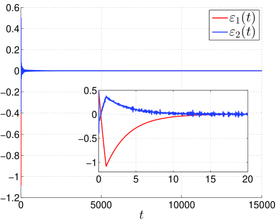
Figure 1: The transients of $\varepsilon(t)=col\{\varepsilon_{1}(t),\varepsilon_{2}(t)\}$.

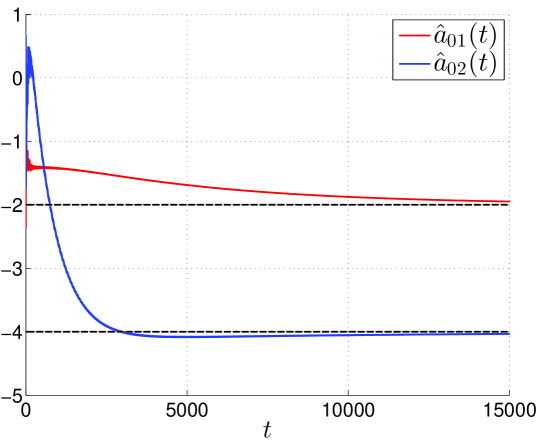
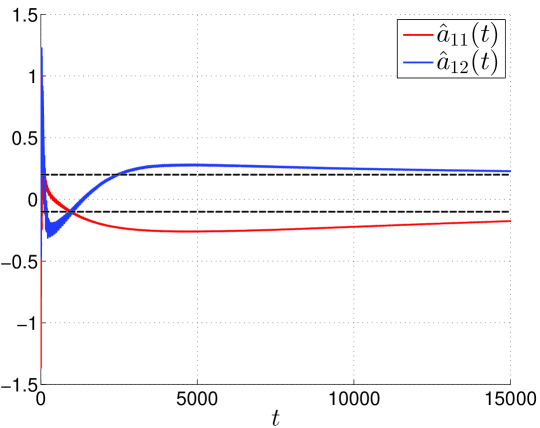
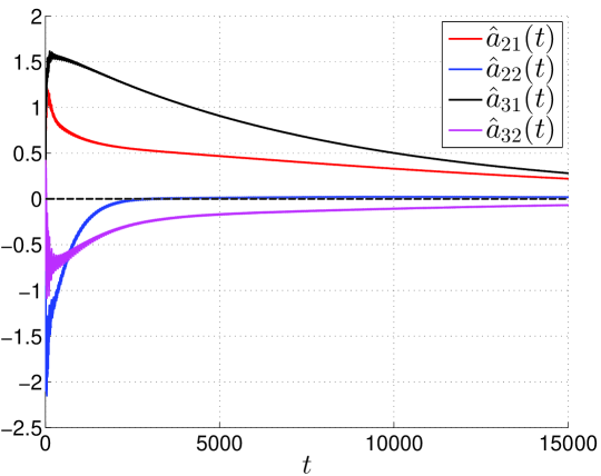
Figure 2: The transients of $\hat{a}_{i1}(t)$, $\hat{a}_{i2}(t)$, $i=0,...,3$, where $a_{01}=-2$, $a_{02}=-4$, $a_{11}=-0.1$, $a_{12}=0.2$, $a_{21}=a_{22}=a_{31}=a_{32}=0$.

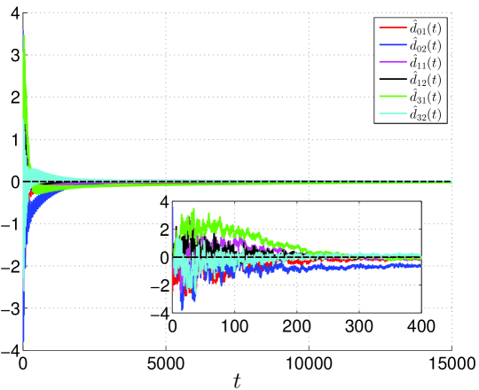
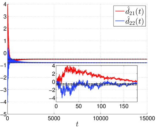
Figure 3: The transients of $\hat{d}_{i1}(t)$, $\hat{d}_{i2}(t)$, $i=0,...,3$, where $d_{21}=-0.5$, $d_{22}=-0.8$, $d_{01}=d_{02}=d_{11}=d_{12}=d_{31}=d_{32}=0$.

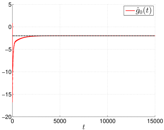
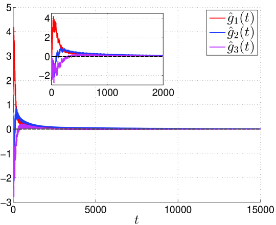
Figure 4: The transients of $\hat{g}_{i}(t)$, $i=0,...,3$, where $g_{0}=-2$, $g_{1}=g_{2}=g_{3}=0$.

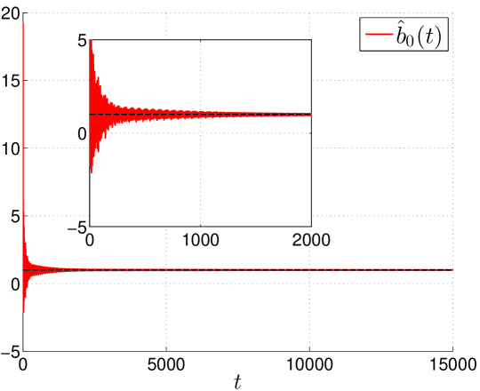
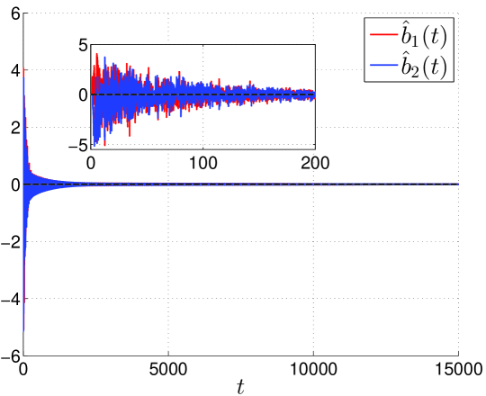
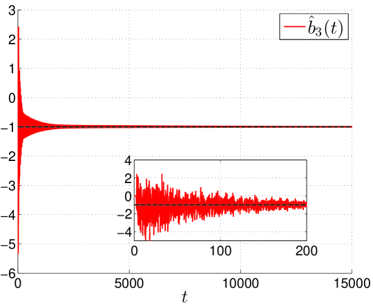
Figure 5: The transients of $\hat{b}_{i}(t)$, $i=0,...,3$, where $b_{0}=1$, $b_{1}=b_{2}=0$, and $b_{3}=-1$.

6 Conclusions

In the paper, a novel adaptive identifier design is proposed for nonlinear systems composed of linear part, Lipschitz and non-Lipschitz nonlinearities. The case of known time-delay values and that of unknown delays are addressed side by side. In contrast to the existing literature, SISO time delay systems are considered in the general form rather than in the canonical form only. The identifiability and observability properties are coupled to the persistent excitation of the plant model to ensure the asymptotic convergence of estimated parameters to their real values by using the gradient algorithm. The stability analysis is given in terms of the feasibility of certain linear matrix inequalities, relying on input and output matrices. The numerical simulations confirm theoretical results and illustrate efficiency of the proposed algorithm for on-line simultaneous estimation of a large number of unknown parameters, including $2$ state components and $24$ parameters.

References

Astrom and Wittenmark (1989)
Astrom, K.J. and Wittenmark, B. (1989). Adaptive Control. Addison-Wesley, Reading MA.
Belkoura and Orlov (2002)
Belkoura, L. and Orlov, Y. (2002). Identifiability analysis of linear delay-differential systems. IMA Journal of Mathematical
Control and Information, volume 19, 73–81.
Boyd and Vandenberghe (2004)
Boyd, S. and Vandenberghe, L.(2004). Convex Optimization. University Press, Cambridge.
Ekramian et al. (2013)
Ekramian, M., Sheikholeslam, F., Hosseinnia, S., Yazdanpanah, M.J. (2013).
Adaptive state observer for Lipschitz nonlinear systems.
Systems & Control Letters, volume 62, 4, 319–323.
Farza et al. (2009)
Farza, M., M’Saad, M., Maatoug, T., Kamounb, M. (2009).
Adaptive observers for nonlinearly parameterized class of nonlinear systems.
Automatica, volume 45, 10, 2292–2299.
Flah et. al. (2014)
Flah, A., Novak, M., Lassaad, S., and Novak, J. (2014).
Estimation of motor parameters for an electrical vehicle application. Int. J. Modelling, Identification and Control, volume 22, 2, 150–158.
Goodwin and Sin (1984)
Goodwin, G.C. and Sin, K.S. (1984).
Adaptive Filtering Prediction and Control. Prentice-Hall: Englewood Cliffs, NJ.
Henry (1991) Henry, D. (1981) Geometric theory of semilinear parabolic
equations. Lecture Notes in Mathematics, Springer-Verlag, Berlin.
Hovakimyan and Cao (2010)
Hovakimyan, N. and Cao, C. (2010)
L1 Adaptive Control Theory. SIAM.
Ioannou and Sun (1995)
Ioannou, P.A. and Sun, J. (1995).
Robust Adaptive Control. Prentice-Hall: Englewood Cliffs, NJ.
Ioannou (1996)
Ioannou, P.A. and Sun Jung. (1996).
Robust Adaptive Control. Prentice Hall, Upper Saddle River.
Kumar et al. (2019)
Kumar, M., Prasad, D., Giri, B.S., and Singh, R.S. (2019).
Temperature control of fermentation bioreactor for ethanol production using IMC-PID controller. Biotechnol Rep (Amst)., doi: 10.1016/j.btre.2019.e00319.
Landau (1979)
Landau, Y.D. (1979).
Adaptive Control – The Model Reference Approach. Marcel Dekker: New York.
Ljung (1999)
Ljung, L. (1999).
System Identification. Theory for the User. 2nd ed. PTR Prentice Hall, Upper Saddle River.
Mareels and Gevers (1988)
Mareels, I.M.Y. and Gevers, M. (1988).
Persistency of Excitation Criteria for
Linear, Multivariable, Time-Varying Systems. Mathematics of Control,
Signals, and Systems, volume 1, 203–226.
Nakagiri and Yamamoto (1995)
Nakagiri, S.I. and Yamamoto, M. (1995).
Unique identification of coefficient matrices, time delay and initial function of
functional differential equations. Journal of Mathematical Systems, volume 5, 3, 323–344.
Narendra and Annaswamy (1989)
Narendra, K.S. and Annaswamy, A. (1989). Stable Adaptive Systems. Prentice-Hall: Englewood Cliffs, NJ, 1989.
Orlov et al. (2001)
Orlov, Y., Belkoura, L., Richard, J.P., and Dambrine, M. (2001). Identifiability analysis of linear time delay systems. Proc. of
the 40th IEEE Conference on Decision and Control, Orlando, USA, 4776–4781.
Orlov et al. (2002)
Orlov, Y., Belkoura, L., Richard, J.-P., and Dambrine, M. (2002). On identifiability of linear time-delay systems. IEEE Transactions
on Automatic Control, volume 47, 8.
Orlov et al. (2003)
Orlov, Y., Belkoura, L., Richard, J.-P., and Dambrine,M. (2003). Adaptive identification of linear time-delay systems. Int. J. Robust Nonlinear Control, volume 13, 857–872.
Orlov et al. (2009)
Orlov, Y., Kolmanovsky, I.V., and Gomez, O. (2009). Adaptive identification of linear time-delay systems: From theory toward application to engine transient fuel identification. Int. J. Adapt. Control Signal Processing, volume 23, 150–165.
Rouche et al. (1977) Rouche, N., Habets, P., Laloy, M. (1977). Stability theory by Lyapunov’s direct method. Springer Verlag, New York.
Sastry and Bodson (1989)
Sastry, S.S. and Bodson, M. (1989). Adaptive Control: Stability, Convergence and Robustness. Prentice-Hall: Englewood Cliffs, NJ.
Shimkin and Feuer (1987)
Shimkin, N. and Feuer, A. (1987). Persistency of Excitation in Continuous-Time
Systems. Systems and Control Letters, volume 9, 225–233.
Tao (2003)
Tao, G. (2003). Adaptive Control Design and Analysis. John Wiley & Sons,
Inc., NY.
Verduyn (2001)
Verduyn Lunel, S.M. (2001). Parameter identifiability of differential delay equations. Adaptive Control and Signal Processing, volume 15, 6, 655–678.
Yakubovich (1973)
Yakubovich, V.A. (1973).
A frequency theorem in control theory. Siberian Mathematical Journal, volume 14, 2, 265–289.