Edge-Weighted Online Bipartite Matching

Online bipartite matching and its variants are among the most fundamental problems in the online algorithms literature. Karp, Vazirani, and Vazirani (STOC 1990) introduced an elegant algorithm for the unweighted problem that achieves an optimal competitive ratio of $1-\nicefrac{{1}}{{e}}$. Later, Aggarwal et al. (SODA 2011) generalized their algorithm and analysis to the vertex-weighted case. Little is known, however, about the most general edge-weighted problem aside from the trivial $\nicefrac{{1}}{{2}}$-competitive greedy algorithm. In this paper, we present the first online algorithm that breaks the long-standing $\nicefrac{{1}}{{2}}$ barrier and achieves a competitive ratio of at least $0.5086$. In light of the hardness result of Kapralov, Post, and Vondrák (SODA 2013) that restricts beating a $\nicefrac{{1}}{{2}}$ competitive ratio for the more general problem of monotone submodular welfare maximization, our result can be seen as strong evidence that edge-weighted bipartite matching is strictly easier than submodular welfare maximization in the online setting.

The main ingredient in our online matching algorithm is a novel subroutine called online correlated selection (OCS), which takes a sequence of pairs of vertices as input and selects one vertex from each pair. Instead of using a fresh random bit to choose a vertex from each pair, the OCS negatively correlates decisions across different pairs and provides a quantitative measure on the level of correlation. We believe our OCS technique is of independent interest and will find further applications in other online optimization problems.

1 Introduction

Matchings are fundamental structures in graph theory that play an indispensable role in combinatorial optimization. For decades, there have been tremendous and ongoing efforts to design more efficient algorithms for finding maximum matchings in terms of their cardinality, and more generally, their total weight. In particular, matchings in bipartite graphs have found countless applications in settings where it is desirable to assign entities from one set to those in another set (e.g., matching students to schools, physicians to hospitals, computing tasks to servers, and impressions in online media to advertisers). Due to the enormous growth of matching markets in digital domains, efficient online matching algorithms have become increasingly important. In particular, search engine companies have created opportunities for online matching algorithms to have a massive impact in multibillion-dollar advertising markets. Motivated by these applications, we consider the problem of matching a set of impressions that arrive one by one to a set of advertisers that are known in advance. When an impression arrives, its edges to the advertisers are revealed and an irrevocable decision has to be made about to which advertiser the impression should be assigned. Karp, Vazirani, and Vazirani [27] gave an elegant online algorithm called Ranking to find matchings in unweighted bipartite graphs with a competitive ratio of $1-\nicefrac{{1}}{{e}}$. They also proved that this is the best achievable competitive ratio. Further, Aggarwal et al. [1] generalized their algorithm to the vertex-weighted online bipartite matching problem and showed that the $1-\nicefrac{{1}}{{e}}$ competitive ratio is still attainable.

The edge-weighted case, however, is much more nebulous. This is partly due to the fact that no competitive algorithm exists without an additional assumption. To see this, consider two instances of the edge-weighted problem, each with one advertiser and two impressions. The edge weight of the first impression is $1$ in both instances, and the weight of the second impression is $0$ in the first instance and $W$ in the second instance, for some arbitrarily large $W$. An online algorithm cannot distinguish between the two instances when the first impression arrives, but it has to decide whether or not to assign this impression to the advertiser. Not assigning it gives a competitive ratio of $0$ in the first instance, and assigning it gives an arbitrarily small competitive ratio of $\nicefrac{{1}}{{W}}$ in the second. This problem cannot be tackled unless assigning both impressions to the advertiser is an option.

In display advertising, assigning more impressions to an advertiser than they paid for only makes them happier. In other words, we can assign multiple impressions to any given advertiser. However, instead of achieving the weights of all the edges assigned to it, we only acknowledge the maximum weight (i.e., the objective equals the sum of the heaviest edge weight assigned to each advertiser). This is equivalent to allowing the advertiser to dispose of previously matched edges for free to make room for new, heavier edges. This assumption is commonly known as the free disposal model. In the display advertising literature [8, 23], the free-disposal assumption is well received and widely applied because of its natural economic interpretation. Finally, edge-weighted online bipartite matching with free disposal is a special case of the monotone submodular welfare maximization problem, where we can apply known $\nicefrac{{1}}{{2}}$-competitive greedy algorithms [10, 28].

1.1 Our Contributions

Despite thirty years of research in online matching since the seminal work of Karp et al. [27], finding an algorithm for edge-weighted online bipartite matching that achieves a competitive ratio greater than $\nicefrac{{1}}{{2}}$ has remained a tantalizing open problem. This paper gives a new online algorithm and answers the question affirmatively, breaking the long-standing $\nicefrac{{1}}{{2}}$ barrier (under free disposal).

Theorem 1.

There is a 0.5086-competitive algorithm for edge-weighted online bipartite matching.

Given the hardness result of Kapralov, Post, and Vondrák [26] that restricts beating a competitive ratio of $\nicefrac{{1}}{{2}}$ for monotone submodular welfare maximization, our algorithm shows that edge-weighted bipartite matching is strictly easier than submodular welfare maximization in the online setting.

From now on, we will use the more formal terminologies of offline and online vertices in a bipartite graph instead of advertisers and impressions. One of our main technical contributions is a novel algorithmic ingredient called online correlated selection (OCS), which is an online subroutine that takes a sequence of pairs of vertices as input and selects one vertex from each pair. Instead of using a fresh random bit to make each of its decisions, the OCS asks to what extent the decisions across different pairs can be negatively correlated, and ultimately guarantees that a vertex appearing in $k$ pairs is selected at least once with probability strictly greater than $1-2^{-k}$. See Section 3 for a short introduction and Section 5 for the full details.

Given an OCS, we can achieve a better than $\nicefrac{{1}}{{2}}$ competitive ratio for unweighted online bipartite matching with the following (barely) randomized algorithm. For each online vertex, either pick a pair of offline neighbors and let the OCS select one of them, or choose one offline neighbor deterministically. More concretely, among the neighbors that have not been matched deterministically, find the least-matched ones (i.e., those that have appeared in the least number of pairs). Pick two if there are at least two of them; otherwise, choose one deterministically. We analyze this algorithm in Appendix A.

Although the competitive ratio of the algorithm above is far worse than the optimal $1-\nicefrac{{1}}{{e}}$ ratio by Karp et al. [27], it benefits from improved generalizability. To extend this algorithm to the edge-weighted problem, we need a reasonable notion of “least-matched” offline neighbors. Suppose one neighbor’s heaviest edge weight is either $1$ or $4$ each with probability $\nicefrac{{1}}{{2}}$, another neighbor’s heaviest edge is $2$ with certainty, and their edge weights with the current online vertex are both $3$. Which one is less matched? To remedy this, we use the online primal-dual framework for matching problems by Devanur, Jain, and Kleinberg [5], along with an alternative formulation of the edge-weighted online bipartite matching problem by Devanur et al. [4]. In short, we account for the contribution of each offline vertex by weight-levels, and at each weight-level we consider the probability that the heaviest edge matched to the vertex has weight at least this level. This is the complementary cumulative distribution function (CCDF) of the heaviest edge weight, and hence we call this the CCDF viewpoint. Then for each offline neighbor, we utilize the dual variables to compute an offer at each weight-level, should the current online vertex be matched to it. The neighbor with the largest net offer aggregating over all weight-levels is considered the “least-matched”. We introduce the online primal-dual framework and the CCDF viewpoint in Section 2. Then we formally present our edge-weighted matching algorithm in Section 4, followed by its analysis. Lastly, Appendix B includes hard instances that show the competitive ratio of our algorithm is nearly tight.

1.2 Related Works

The literature of online weighted bipartite matching algorithms is extensive, but most of these works are devoted to achieving competitive ratios greater than $\nicefrac{{1}}{{2}}$ by assuming that offline vertices have large capacities or that some stochastic information about the online vertices is known in advance. Below we list the most relevant works and refer interested readers to the excellent survey of Mehta [29]. We note that there have recently been several significant advances in more general settings, including different arrival models and general (non-bipartite) graphs [15, 13, 12, 17].

Large Capacities.

The capacity of an offline vertex is the number of online vertices that can be assigned to it. Exploiting the large-capacity assumption to beat $\nicefrac{{1}}{{2}}$ dates back two decades ago to Kalyanasundaram and Pruhs [25]. Feldman et al. [8] gave a $(1-\nicefrac{{1}}{{e}})$-competitive algorithm for Display Ads, which is equivalent to edge-weighted online bipartite matching assuming large capacities. Under similar assumptions, the same competitive ratio was obtained for AdWords [33, 2], in which offline vertices have some budget constraint on the total weight that can be assigned to them rather than the number of impressions. From a theoretical point of view, one of the primary goals in the online matching literature is to provide algorithms with competitive ratio greater than $\nicefrac{{1}}{{2}}$ without making any assumption on the capacities of offline vertices.

Stochastic Arrivals.

If we have knowledge about the arrival patterns of online vertices, we can often leverage this information to design better algorithms. Typical stochastic assumptions include assuming the online vertices are drawn from some known or unknown distribution [9, 22, 6, 16, 30, 32, 21], or that they arrive in a random order [14, 3, 7, 35, 31, 34, 19]. These works achieve a $1-\varepsilon$ competitive ratio if the large capacity assumption holds in addition to the stochastic assumptions, or at least $1-\nicefrac{{1}}{{e}}$ for arbitrary capacities. Korula, Mirrokni, and Zadimoghaddam [24] showed that the greedy algorithm is $0.505$-competitive for the more general problem of submodular welfare maximization if the online vertices arrive in a random order, without any assumption on the capacities. The random order assumption is particularly justified because Kapralov et al. [26] proved that beating $\nicefrac{{1}}{{2}}$ for submodular welfare maximization in the oblivious adversary model implies $\textbf{NP}=\textbf{RP}$.

2 Preliminaries

The edge-weighted online matching problem considers a bipartite graph $G=(L,R,E)$, where $L$ and $R$ are the sets of vertices on the left-hand side (LHS) and right-hand side (RHS), respectively, and $E\subseteq L\times R$ is the set of edges. Every edge $(i,j)\in E$ is associated with a nonnegative weight $w_{ij}\geq 0$, and we can assume without loss of generality that this is a complete bipartite graph, i.e., $E=L\times R$, by assigning zero weights to the missing edges.

The vertices on the LHS are offline in that they are all known to the algorithm in advance. The vertices on the RHS, however, arrive online one at a time. When an online vertex $j\in R$ arrives, its incident edges and their weights are revealed to the algorithm, who must then irrevocably match $j$ to an offline neighbor. Each offline vertex can be matched any number of times, but only the weight of its heaviest edge counts towards the objective. This is equivalent to allowing a matched offline vertex $i$, say, to $j$, to be rematched to a new online vertex $j^{\prime}$ with edge weight $w_{ij^{\prime}}>w_{ij}$, disposing of vertex $j$ and edge $(i,j)$ for free. This assumption is known as the free disposal model.

The goal is to maximize the total weight of the matching. A randomized algorithm is $\Gamma$-competitive if its expected objective value is at least $\Gamma$ times the offline optimal in hindsight, for any instance of edge-weighted online matching. We refer to $0\leq\Gamma\leq 1$ as the competitive ratio of the algorithm.

2.1 Complementary Cumulative Distribution Function Viewpoint

Next we describe an alternative formulation of the edge-weighted online matching problem due to Devanur et al. [4] that captures the contribution of each offline vertex $i\in L$ to the objective in terms of the complementary cumulative distribution function (CCDF) of the heaviest edge weight matched to $i$. We refer to this approach as the CCDF viewpoint.

For any offline vertex $i\in L$ and any weight-level $w\geq 0$, let $y_{i}(w)$ be CCDF of the weight of the heaviest edge matched to $i$, i.e., the probability that $i$ is matched to at least one online vertex $j$ such that $w_{ij}\geq w$. Then, $y_{i}(w)$ is a non-increasing function of $w$ that takes values between $0$ and $1$. Observe that $y_{i}(w)$ is a step function with polynomially many pieces, because the number of pieces is at most the number of incident edges. Hence, we will be able to maintain $y_{i}(w)$ in polynomial time.

The expected weight of the heaviest edge matched to $i$ then equals the area under $y_{i}(w)$, i.e.:

$$\int_{0}^{\infty}y_{i}(w)dw\leavevmode\nobreak\ .$$ (1)

This follows from an alternative formula for the expected value of a nonnegative random variable involving only its cumulative distribution function.

We illustrative this idea with an example in Figure 1. Suppose an offline vertex $i$ has four online neighbors $j_{1}$, $j_{2}$, $j_{3}$, and $j_{4}$ with edge weights $w_{1}<w_{2}<w_{3}<w_{4}$. Further, suppose that $j_{1}$ is matched to $i$ with certainty, while $j_{2}$, $j_{3}$, and $j_{4}$ each have some probability of being matched to $i$. (The latter events may be correlated.) Next, suppose a new neighbor arrives whose edge weight is also $w_{3}$. The values of $y_{i}(w)$ are then increased for $w_{1}<w\leq w_{3}$ accordingly, and the total area of the shaded regions is the increment in the expected weight of the heaviest edge matched to vertex $i$.

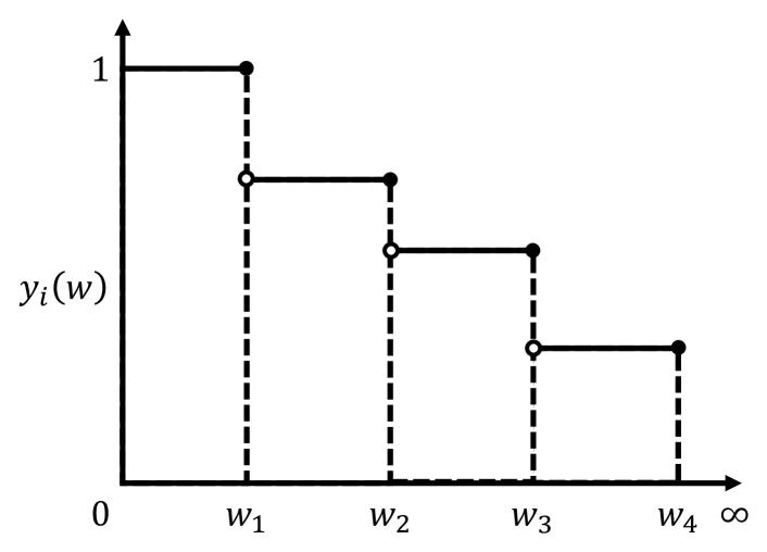
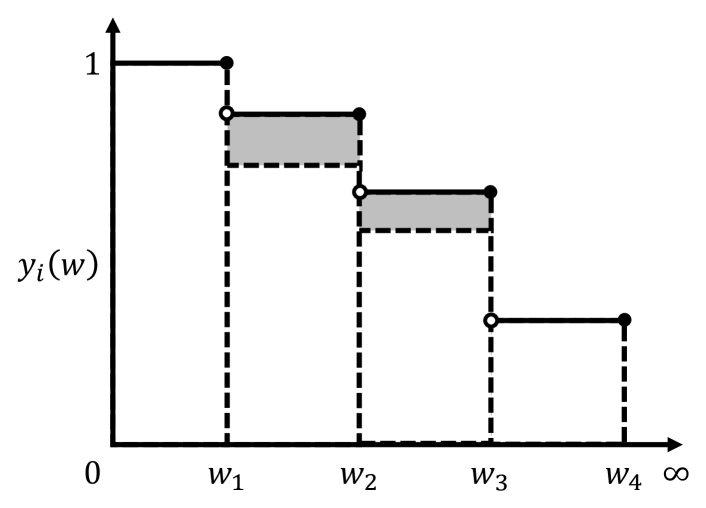
Figure 1: Complementary cumulative distribution function (CCDF) viewpoint. The first function is the CCDF of vertex $i$, and the second function demonstrates how the CCDF of vertex $i$ is updated.

2.2 Online Primal-Dual Framework

We analyze our algorithms using a linear program (LP) for edge-weighted matching under the online primal-dual framework. Consider the standard matching LP and its dual below. We interpret the primal variables $x_{ij}$ as the probability that $(i,j)$ is the heaviest edge matched to vertex $i$. $\displaystyle\max\quad$ $\displaystyle\sum_{i\in L}\sum_{j\in R}w_{ij}x_{ij}$ s.t. $\displaystyle\sum_{j\in R}x_{ij}\leq 1$ $\displaystyle\forall i\in L$ $\displaystyle\sum_{i\in L}x_{ij}\leq 1$ $\displaystyle\forall j\in R$ $\displaystyle x_{ij}\geq 0$ $\displaystyle\forall i\in L,\forall j\in R$ $\displaystyle\min\quad$ $\displaystyle\sum_{i\in L}\alpha_{i}+\sum_{j\in R}\beta_{j}$ s.t. $\displaystyle\alpha_{i}+\beta_{j}\geq w_{ij}$ $\displaystyle\forall i\in L,\forall j\in R$ $\displaystyle\alpha_{i}\geq 0$ $\displaystyle\forall i\in L$ $\displaystyle\beta_{j}\geq 0$ $\displaystyle\forall j\in R$

Let P denote the primal objective. If $x_{ij}$ is the probability that $(i,j)$ is the heaviest edge matched to $i$, then P also equals the objective of the algorithm. Let D denote the dual objective.

Online algorithms under the online primal-dual framework maintain not only a matching but also a dual assignment (not necessarily feasible) at all times subject to the conditions summarized below.

Lemma 2.

Suppose an online algorithm simultaneously maintains primal and dual assignments such that for some constant $0\leq\Gamma\leq 1$, the following conditions hold at all times:

1. Approximate dual feasibility:  For any $i\in L$ and any $j\in R$, we have $\alpha_{i}+\beta_{j}\geq\Gamma\cdot w_{ij}$.

2. Reverse weak duality:  The objectives of the primal and dual assignments satisfy $\textsc{P}\geq\textsc{D}$.

Then, the algorithm is $\Gamma$-competitive.

Proof.

By the first condition, the values $\Gamma^{-1}\alpha_{i}$ and $\Gamma^{-1}\beta_{j}$ form a feasible dual assignment whose objective equals $\Gamma^{-1}\textsc{D}$. By weak duality of linear programming, the objective of any feasible dual assignment upper bounds the optimal (i.e., D is at least $\Gamma$ times the optimal). Applying the second condition now proves the lemma. ∎

Online Primal-Dual in the CCDF Viewpoint.

In light of the CCDF viewpoint, for any offline vertex $i\in L$ and any weight-level $w>0$, we introduce and maintain new variables $\alpha_{i}(w)$ that satisfy:

$$\alpha_{i}=\int_{0}^{\infty}\alpha_{i}(w)dw\leavevmode\nobreak\ .$$ (2)

Accordingly, we rephrase approximate dual feasibility in Lemma 2 in the CCDF viewpoint as:

$$\int_{0}^{\infty}\alpha_{i}(w)dw+\beta_{j}\geq\Gamma\cdot w_{ij}\leavevmode\nobreak\ .$$ (3)

Concretely, at each step of our primal-dual algorithm, $\alpha_{i}(w)$ is a piecewise constant function with possible discontinuities at the weight-levels $w\in\{w_{ij}\in E:\text{online vertex $j$ has arrived}\}$. Initially, all of the $\alpha_{i}(w)$’s are the zero function. Then, as each online vertex $j\in R$ arrives, if $j$ is potentially matched to an offline candidate $i\in L$, the function values of $\alpha_{i}(w)$ are systematically increased according to the dual update rules in Section 4.1. In contrast, each dual variable $\beta_{j}$ is a scalar value that is initialized to zero and increased only once during the algorithm, at the time when $j$ arrives.

3 Online Correlated Selection: An Introduction

This section introduces our novel ingredient for online algorithms, which we believe to be widely-applicable and of independent interest. To motivate this technique, consider the following thought experiment in the case of unweighted online matching, i.e., $w_{ij}\in\{0,1\}$ for any $i\in L$ and any $j\in R$.

Deterministic Greedy.

We first recall why all deterministic greedy algorithms that match each online vertex to an unmatched offline neighbor are at most $\nicefrac{{1}}{{2}}$-competitive. Consider an instance with a graph that has two offline and two online vertices. The first online vertex is adjacent to both offline vertices, and the algorithm deterministically chooses one of them. The second online vertex, however, is only adjacent to the previously matched vertex.

Two-Choice Greedy with Independent Random Bits.

We can avoid the problem above by matching the first online vertex randomly, which improves the expected matching size from $1$ to $1.5$. In this spirit, consider the following two-choice greedy algorithm. When an online vertex arrives, identify its neighbors that are least likely to be matched (over the randomness in previous rounds). If there is more than one such neighbor, choose any two, e.g., lexicographically, and match to one with a fresh random bit. Otherwise, match to the least-matched neighbor deterministically. We refer to the former as a randomized round and the latter as a deterministic round. Since each randomized round uses a fresh random bit, this is equivalent to matching to neighbors that have been chosen in the least number of randomized rounds and in no deterministic round. Unfortunately, this algorithm is also $\nicefrac{{1}}{{2}}$-competitive due to upper triangular graphs. We defer this standard example to Appendix B.

Two-choice Greedy with Perfect Negative Correlation.

The last algorithm in this thought experiment is an imaginary variant of two-choice greedy that perfectly and negatively correlates the randomized rounds so that each offline vertex is matched with certainty after being a candidate in two randomized rounds. This is infeasible in general. Nevertheless, if we assume feasibility then this algorithm is $\nicefrac{{5}}{{9}}$-competitive [18]. In fact, it is effectively the $2$-matching algorithm of Kalyanasundaram and Pruhs [25], by having two copies of each online vertex and allowing offline vertices to be matched twice.

Can we use partial negative correlation to retain feasibility and break the $\nicefrac{{1}}{{2}}$ barrier?

We answer this question affirmatively by introducing an algorithmic ingredient called online correlated selection (OCS), which allows us to quantify the negative correlation among randomized rounds. Appendix A provides an analysis of the two-choice greedy algorithm powered by OCS in the unweighted case. Furthermore, Section 4 generalizes this approach to edge-weighted online matching, achieving the first algorithm with a competitive ratio that is provably greater than $\nicefrac{{1}}{{2}}$.

Definition 1 ($\gamma$-semi-OCS).

Consider a set of ground elements. For any $\gamma\in[0,1]$, a $\gamma$-semi-OCS is an online algorithm that takes as input a sequence of pairs of elements, and selects one per pair such that if an element appears in $k\geq 1$ pairs, it is selected at least once with probability at least:

$$1-2^{-k}(1-\gamma)^{k-1}\leavevmode\nobreak\ .$$

Using independent random bits is a $0$-semi-OCS, and the perfect negative correlation in the thought experiment corresponds to a $1$-semi-OCS, although it is typically infeasible. Our algorithms satisfy a stronger definition, which considers any collection of pairs containing an element $i$. This stronger definition is useful for generalizing to the edge-weighted bipartite matching problem.

In the following definition, a subsequence (not necessarily contiguous) of pairs containing element $i$ is consecutive if it includes all the pairs that contain element $i$ between the first and last pair in the subsequence. Further, two subsequences of pairs are disjoint if no pair belongs to both of them. For example, consider the sequence $(\{a,i\},\{b,i\},\{c,d\},\{e,i\},\{i,z\})$. The subsequences $(\{a,i\},\{b,i\})$ and $(\{i,z\})$ are consecutive and disjoint, but the subsequence $(\{a,i\},\{b,i\},\{i,z\})$ is not consecutive because it does not include the pair $\{e,i\}$.

Definition 2 ($\gamma$-OCS).

Consider a set of ground elements. For any $\gamma\in[0,1]$, a $\gamma$-OCS is an online algorithm that takes as input a sequence of pairs of elements, and selects one per pair such that for any element $i$ and any disjoint subsequences of $k_{1},k_{2},\dots,k_{m}$ consecutive pairs containing $i$, $i$ is selected in at least one of these pairs with probability at least:

$$1-\prod_{\ell=1}^{m}2^{-k_{\ell}}(1-\gamma)^{k_{\ell}-1}\leavevmode\nobreak\ .$$

Theorem 3.

There exists a $\frac{13\sqrt{13}-35}{108}>0.1099$-OCS.

We defer the design and analysis of this OCS to Section 5, and instead describe a weaker $\nicefrac{{1}}{{16}}$-OCS, which is already sufficient for breaking the $\nicefrac{{1}}{{2}}$ barrier in edge-weighted online bipartite matching.

Proof Sketch of a $\nicefrac{{1}}{{16}}$-OCS.

Consider two sequences of random bits. The first set is used to construct a random matching among the pairs, where any two consecutive pairs (with respect to some element) are matched with probability $\nicefrac{{1}}{{16}}$. Concretely, each pair is consecutive to at most four pairs, one before it and one after it for each of its two elements. For each pair, choose one of its consecutive pairs, each with probability $\nicefrac{{1}}{{4}}$. Two consecutive pairs are matched if they choose each other.

The second random sequence is used to select elements from the pairs. For any unmatched pair, choose one of its elements with a fresh random bit. For any two matched pairs, use a fresh random bit to choose an element in the first pair, and then make the opposite selection for the later one (i.e., select the common element if it is not selected in the earlier pair, and vice versa). Observe that even if two matched pairs are identical, there is no ambiguity in the opposite selection.

Next, fix any element $i$ and any disjoint subsequences of $k_{1},k_{2},\dots,k_{m}$ consecutive pairs containing $i$. We bound the probability that $i$ is never selected. If any two of the pairs are matched, $i$ is selected once in the two pairs. Otherwise, the selections from the pairs are independent, and the probability that $i$ is never selected is $\prod_{\ell=1}^{m}2^{-k_{\ell}}$. Applying the law of total probability to the event that $i$ is in a matched pair, it remains to upper bound the probability of having no such matched pairs by $\prod_{\ell=1}^{m}(1-\nicefrac{{1}}{{16}})^{k_{\ell}-1}$. Intuitively, this is because there are $k_{\ell}-1$ choices of two consecutive pairs within the $\ell$-th subsequence, each of which is matched with probability $\nicefrac{{1}}{{16}}$. Further, these events are negatively dependent and therefore, the probability that none of them happens is upper bounded by the independent case. The formal analysis in Section 5 substantiates this claim. ∎

4 Edge-Weighted Online Matching

This section presents an online primal-dual algorithm for the edge-weighted online bipartite matching problem. The algorithm uses a $\gamma$-OCS as a black box, and its competitive ratio depends on the value of $\gamma$. For $\gamma=\nicefrac{{1}}{{16}}$ (as sketched in Section 3) it is $0.505$-competitive, and for $\gamma\approx 0.1099$ (as in Theorem 3) it is $0.5086$-competitive, proving our main result about edge-weighted online matching.

4.1 Online Primal-Dual Algorithm

The algorithm is similar to the two-choice greedy in the previous section. It maintains an OCS with the offline vertices as the ground elements. For each online vertex, the algorithm either (1) matches it deterministically to one offline neighbor, (2) chooses a pair of offline neighbors and matches to the one selected by the OCS, or (3) leaves it unmatched. We refer to the first case as a deterministic round, the second as a randomized round, and the third as an unmatched round.

How does the algorithm decide whether it is a randomized, deterministic or unmatched round, and how does it choose the candidate offline vertices? We leverage the online primal-dual framework. When an online vertex $j$ arrives, it calculates for every offline vertex $i$ how much the dual variable $\beta_{j}$ would gain if $j$ is matched to $i$ in a deterministic round, denoted as $\Delta_{i}^{D}\beta_{j}$, and similarly $\Delta_{i}^{R}\beta_{j}$ for a randomized round. Then it finds $i^{*}$ with the maximum $\Delta_{i}^{D}\beta_{j}$, and $i_{1},i_{2}$ with the maximum $\Delta_{i}^{R}\beta_{j}$. If both $\Delta_{i_{1}}^{R}\beta_{j}+\Delta_{i_{2}}^{R}\beta_{j}$ and $\Delta_{i^{*}}^{D}\beta_{j}$ are negative, it leaves $j$ unmatched. If $\Delta_{i_{1}}^{R}\beta_{j}+\Delta_{i_{2}}^{R}\beta_{j}$ is nonnegative and greater than $\Delta_{i^{*}}^{D}\beta_{j}$, it matches $j$ in a randomized round with $i_{1}$ and $i_{2}$ as the candidates using its OCS. Finally, if $\Delta_{i^{*}}^{D}\beta_{j}$ is nonnegative and greater than $\Delta_{i_{1}}^{R}\beta_{j}+\Delta_{i_{2}}^{R}\beta_{j}$, it matches $j$ to $i^{*}$ in a deterministic round. See Algorithm 1 for the formal definition of the algorithm.

It remains to explain how $\Delta_{i}^{D}\beta_{j}$ and $\Delta_{i}^{R}\beta_{j}$ are calculated. For any offline vertex $i\in L$ and any weight-level $w>0$, let $k_{i}(w)$ be the number of randomized rounds in which $i$ has been chosen and has edge weight at least $w$. The values of $k_{i}(w)$ may change over time, so we consider these values at the beginning of each online round. The increments to the dual variables $\alpha_{i}(w)$ and $\beta_{j}$ depend on the values of $k_{i}(w)$ via the following gain-sharing parameters, which we determine later using a factor-revealing LP to optimize the competitive ratio. The gain-sharing values are listed at the end of this section in Table 1.

• $a(k)$ : Amortized increment in the dual variable $\alpha_{i}(w)$ if $i$ is chosen as one of the two candidates in a randomized round in which its edge weight is at least $w$ and $k_{i}(w)=k$.

• $b(k)$ : Increment in the dual variable $\beta_{j}$ due to an offline vertex $i$ at weight-level $w\leq w_{ij}$ if $j$ is matched in a randomized round with $i$ as one of the two candidates and $k_{i}(w)=k$.

Note that these gain-sharing values $a(k)$ and $b(k)$ are instance independent (i.e., they do not depend on the underlying graph) and defined for all $k\in\mathbb{Z}_{\geq 0}$. We interpret these parameters according to a gain-splitting rule. If $i$ is one of the two candidates to be matched to $j$ in a randomized round, the increase in the expected weight of the heaviest edge matched to $i$ equals the integration of $y_{i}(w)$’s increments, for $0<w\leq w_{ij}$, which can be related to the values of the $k_{i}(w)$’s. We then lower bound the gain due to the increment of $y_{i}(w)$ using the definition of a $\gamma$-OCS and split the gain into two parts, $a(k_{i}(w))$ and $b(k_{i}(w))$. The former is assigned to $\alpha_{i}(w)$ and the latter goes to $\beta_{j}$.

Algorithm 1 Online primal-dual edge-weighted bipartite matching algorithm.

State variables:

• $k_{i}(w)\geq 0$ : The number of randomized rounds in which $i$ is a candidate and its edge weight is at least $w$; $k_{i}(w)=\infty$ if it has been chosen in a deterministic round in which its edge weight is at least $w$.

On the arrival of an online vertex $j\in R$:

1. For every offline vertex $i\in L$, compute $\Delta_{i}^{R}\beta_{j}$ and $\Delta_{i}^{D}\beta_{j}$ according to Eqn. (5) and (6).

2. Find $i_{1},i_{2}$ with the maximum $\Delta_{i}^{R}\beta_{j}$.

3. Find $i^{*}$ with the maximum $\Delta_{i}^{D}\beta_{j}$.

4. If $0>\Delta_{i_{1}}^{R}\beta_{j}+\Delta_{i_{2}}^{R}\beta_{j}$ and $\Delta_{i^{*}}^{D}\beta_{j}$, leave $j$ unmatched. (unmatched)

5. If $\Delta_{i_{1}}^{R}\beta_{j}+\Delta_{i_{2}}^{R}\beta_{j}\geq\Delta_{i^{*}}^{D}\beta_{j}$ and $0$, let the OCS pick one of $i_{1}$ and $i_{2}$. (randomized)

6. If $\Delta_{i^{*}}^{D}\beta_{j}>\Delta_{i_{1}}^{R}\beta_{j}$ and $\geq 0$, match $j$ to $i^{*}$. (deterministic)

7. Update the $k_{i}(w)$’s accordingly.

In fact, we prove at the end of this subsection the following invariant about how the dual variables $\alpha_{i}(w)$ are incremented:

$$\alpha_{i}(w)\geq\sum_{0\leq\ell<k_{i}(w)}a(\ell)\leavevmode\nobreak\ .$$ (4)

Next, define $\Delta^{R}_{i}\beta_{j}$ to be:

$$\Delta_{i}^{R}\beta_{j}\stackrel{{\scriptstyle\text{def}}}{{=}}\int_{0}^{w_{ij}}b\left(k_{i}(w)\right)dw-\frac{1}{2}\int_{w_{ij}}^{\infty}\sum_{0\leq\ell<k_{i}(w)}a(\ell)dw\leavevmode\nobreak\ .$$ (5)

We should think of $\Delta_{i}^{R}\beta_{j}$ as the increase in the dual variable $\beta_{j}$ due to offline vertex $i$, if $i$ is chosen as one of the two candidates for $j$ in an randomized round. The first term in Eqn. 5 follows from the interpretation of $b(k)$ above (and would be the only term in the unweighted case). The second term is designed to cancel out the extra help we get from the $\alpha_{i}(w)$’s at weight-levels $w>w_{ij}$ in order to satisfy approximate dual feasibility for the edge $(i,j)$. Concretely, if $j$ is matched in a randomized round to two candidates at least as good as $i$, our choice of $b(k)$’s ensures approximate dual feasibility between $i$ and $j$ (i.e., the following inequality holds):

$$\int_{0}^{\infty}\alpha_{i}(w)dw+2\cdot\Delta_{i}^{R}\beta_{j}\geq\Gamma\cdot w_{ij}\leavevmode\nobreak\ .$$

Finally, for some $1<\kappa<2$, define the value of $\Delta_{i}^{D}\beta_{j}$ to be:

$$\Delta_{i}^{D}\beta_{j}\stackrel{{\scriptstyle\text{def}}}{{=}}\kappa\cdot\Delta_{i}^{R}\beta_{j}\\ =\kappa\int_{0}^{w_{ij}}b\left(k_{i}(w)\right)dw-\frac{\kappa}{2}\int_{w_{ij}}^{\infty}\sum_{0\leq\ell<k_{i}(w)}a(\ell)dw\leavevmode\nobreak\ .$$ (6)

For concreteness, readers can assume $\kappa=1.5$. The competitive ratio, however, is insensitive to the choice of $\kappa$ as long as it is neither too close to $1$ nor to $2$. On the one hand, $\kappa>1$ ensures that if the algorithm chooses a randomized round with offline vertex $i_{1}$ and another vertex $i_{2}$ as the candidates, the contribution from $i_{2}$ to $\beta_{j}$ must be at least a $\kappa-1$ fraction of what $i_{1}$ offers; otherwise, the algorithm would have preferred a deterministic round with $i_{1}$ alone. On the other hand, we have $\kappa<2$ because otherwise a randomized round would always be inferior to a deterministic round. We further explain the definitions of $\Delta_{i}^{R}\beta_{j}$ and $\Delta_{i}^{D}\beta_{j}$ in Subsection 4.3, and we demonstrate how their terms interact when proving that the dual assignments always satisfy approximate dual feasibility.

Primal Increments.

We have defined the primal algorithm and, implicitly, how the dual algorithm updates the $\beta_{j}$’s. It remains to define the updates to $\alpha_{i}(w)$’s. Before that, we first need to characterize the primal increment since the dual updates are driven by it. Recall that by the CCDF viewpoint:

$$\textsc{P}=\sum_{i\in L}\int_{0}^{\infty}y_{i}(w)dw\leavevmode\nobreak\ .$$

Since it is difficult to account for the exact CCDF $y_{i}(w)$ due to complicated correlations in the selections, we instead consider a lower bound for it given by the $\gamma$-OCS. A critical observation here is that the decisions made by the primal-dual algorithm are deterministic, except for the randomness in the OCS. In particular, its choices of $i_{1}$, $i_{2}$, $i^{*}$ and the decisions about whether a round is unmatched, randomized, or deterministic are independent of the selections in the OCS and therefore deterministic quantities governed solely by the input graph and arrival order of the online vertices. Hence, we may view the sequence of pairs of candidates as fixed.

For any offline vertex $i$ and any weight-level $w>0$, consider the randomized rounds in which $i$ is a candidate and has edge weight at least $w$. Decompose these rounds into disjoint collections of, say, $k_{1},k_{2},\dots,k_{m}$ consecutive rounds. By Definition 2, vertex $i$ is selected by the $\gamma$-OCS in at least one of these rounds with probability at least:

$$\bar{y}_{i}(w)\stackrel{{\scriptstyle\text{def}}}{{=}}1-\prod_{\ell=1}^{m}2^{-k_{\ell}}\left(1-\gamma\right)^{k_{\ell}-1}\leavevmode\nobreak\ .$$ (7)

Accordingly, we will use the following surrogate primal objective:

$$\bar{\textsc{P}}=\sum_{i\in L}\int_{0}^{\infty}\bar{y}_{i}(w)dw\leavevmode\nobreak\ .$$

Lemma 4.

The primal objective is lower bounded by the surrogate, i.e., $\bar{\textsc{P}}\leq\textsc{P}$.

It will often be more convenient to consider the following characterization of $\bar{y}_{i}(w)$:

• Initially, let $\bar{y}_{i}(w)=0$.

• If $i$ is matched in a deterministic round in which its edge weight is at least $w$, let $\bar{y}_{i}(w)=1$.

• If $i$ is chosen in a randomized round in which its edge weight is at least $w$, further consider $w^{\prime}$, its edge weight in the previous round involving $i$; let $w^{\prime}=0$ if it is the first randomized round involving $i$. Then, decrease the gap $1-\bar{y}_{i}(w)$ by a $\nicefrac{{1}}{{2}}(1-\gamma)$ factor if $w^{\prime}\geq w$, i.e., if it is the second or later pair of a collection of consecutive pairs containing $i$ with edge weight at least $w$; otherwise, decrease $1-\bar{y}_{i}(w)$ by $\nicefrac{{1}}{{2}}$, to account for the $-1$ in the exponent of $1-\gamma$ in Eqn 7.

Lemma 5.

For any offline vertex $i$ and any weight-level $w>0$, we have:

$$1-\bar{y}_{i}(w)\geq 2^{-k_{i}(w)}\left(1-\gamma\right)^{\max\{k_{i}(w)-1,0\}}\leavevmode\nobreak\ .$$

Proof.

Initially, $1-\bar{y}_{i}(w)$ equals $1$. Then, it decreases by $\nicefrac{{1}}{{2}}$ in the first randomized round involving $i$ with edge weight at least $w$, and by at most $\nicefrac{{1}}{{2}}\left(1-\gamma\right)$ in each of the subsequent $k_{i}(w)-1$ rounds. ∎

This is equivalent to a lower bound of the increment in $y_{i}(w)$ in a deterministic round.

Lemma 6.

For any offline vertex $i$ and any weight-level $w>0$, if $i$ is matched in a deterministic round in which its edge weight is at least $w$, the increment in $\bar{y}_{i}(w)$ is at least:

$$2^{-k_{i}(w)}\left(1-\gamma\right)^{\max\{k_{i}(w)-1,0\}}\leavevmode\nobreak\ .$$

Lemma 7.

For any offline vertex $i$ and any weight-level $w>0$, if $i$ is chosen as a candidate in a randomized round in which its edge weight is at least $w$, the increment in $\bar{y}_{i}(w)$ is at least:

$$2^{-k_{i}(w)-1}\left(1-\gamma\right)^{\max\{k_{i}(w)-1,0\}}\leavevmode\nobreak\ .$$

Suppose further that vertex $i$’s edge weight is also at least $w$ in the last randomized round involving $i$. Then, it follows that $k_{i}(w)\geq 1$ and the increment in $\bar{y}_{i}(w)$ is at least:

$$2^{-k_{i}(w)-1}\left(1-\gamma\right)^{k_{i}(w)-1}\left(1+\gamma\right)\leavevmode\nobreak\ .$$

Proof.

By definition, $1-\bar{y}_{i}(w)$ decreases by a factor of either $\nicefrac{{1}}{{2}}(1-\gamma)$ or $\nicefrac{{1}}{{2}}$ in a randomized round, depending on whether vertex $i$’s edge weight is at least $w$ the last time it is chosen in a randomized round. Therefore, the increment in $\bar{y}_{i}(w)$ is either a $\nicefrac{{1}}{{2}}(1+\gamma)$ fraction of $1-\bar{y}_{i}(w)$, or a $\nicefrac{{1}}{{2}}$ fraction. Putting this together with the lower bound for $1-\bar{y}_{i}(w)$ in Lemma 5 proves the lemma. ∎

Dual Updates to Online Vertices.

Consider any online vertex $j\in R$ at the time of its arrival. The dual variable $\beta_{j}$ will only increase at the end of this round, depending on the type of assignment. If $j$ is left unmatched, then the value of $\beta_{j}$ remains zero. If $j$ is matched in a randomized round, set $\beta_{j}=\Delta_{i_{1}}^{R}\beta_{j}+\Delta_{i_{2}}^{R}\beta_{j}$. Lastly, if $j$ is matched in a deterministic round, set $\beta_{j}=\Delta_{i^{*}}^{D}\beta_{j}$.

Dual Updates to Offline Vertices: Proof of Eqn. (4).

Fix any offline vertex $i\in L$. Suppose that $i$ is matched in a deterministic round in which its edge weight is $w_{ij}$. Then, for any weight-level $w>w_{ij}$, the value of $k_{i}(w)$ stays the same, so we leave $\alpha_{i}(w)$ unchanged. On the other hand, for any weight-level $w\leq w_{ij}$, the value of $k_{i}(w)$ becomes $\infty$ by definition. Therefore, to maintain the invariant in Eqn. (4), we increase $\alpha_{i}(w)$ for each weight-level $w\leq w_{ij}$ by:

$$\sum_{\ell=k_{i}(w)}^{\infty}a(\ell)\leavevmode\nobreak\ .$$ (8)

The updates in randomized rounds are more subtle. Suppose $i$ is one of the two candidates in a randomized round in which its edge weight is $w_{ij}$. Further consider $i$’s edge weight the last time it was chosen in a randomized round, denoted as $w^{\prime}$; let $w^{\prime}=0$ if this is the first randomized round involving vertex $i$. Then, $w_{ij}$ and $w^{\prime}$ partition the weight-levels $w>0$ into up to three subsets, each of which requires a different update rule for $\alpha_{i}(w)$. Concretely, the algorithm increase $\alpha_{i}(w)$ by:

$$\begin{cases}a\left(k_{i}(w)\right)&\text{if }0<w\leq w_{ij},w^{\prime}\textrm{ or }k_{i}(w)=0\leavevmode\nobreak\ ;\\ a\left(k_{i}(w)\right)-2^{-k_{i}(w)-1}\left(1-\gamma\right)^{k_{i}(w)-1}\gamma&\text{if }w^{\prime}<w\leq w_{ij}\textrm{ and }k_{i}(w)\geq 1\leavevmode\nobreak\ ;\\ 2^{-k_{i}(w)-1}\left(1-\gamma\right)^{k_{i}(w)-1}\gamma&\text{if }w>w_{ij}\textrm{ and }k_{i}(w)\geq 1\leavevmode\nobreak\ .\end{cases}$$ (9)

The first case is straightforward—we simply increase $\alpha_{i}(w)$ by $a\left(k_{i}(w)\right)$ to maintain the invariant in Eqn. (4). Observe that this is the only case in the unweighted problem.

For a weight-level $w$ that falls into the second case (if there is any), the increment in $\alpha_{i}(w)$ is smaller than the first case by $2^{-k_{i}(w)-1}(1-\gamma)^{k_{i}(w)-1}\gamma$. This is the difference between the lower bounds for the increments in $\bar{y}_{i}(w)$ in Lemma 7, depending on whether $i$’s edge weight was at least $w$ the last time it was chosen in a randomized round. Since the increase in the surrogate primal objective $\bar{\textsc{P}}$ due to vertex $i$ and weight-level $w$ (when $w^{\prime}<w$) is less than the first case of Eqn. (9), we subtract this difference from the increment in $\alpha_{i}(w)$ so that the update to $\beta_{j}$ is unaffected.

How can we still maintain the invariant in Eqn. (4) given the subtraction in the second case? Observe that if the second case happens, the same weight-level must fall into the third case in the previous randomized round in which $i$ is involved. Thus, an equal amount is prepaid to each $\alpha_{i}(w)$ in the previous round. This give-and-take in the offline dual vertex updates becomes clear when we prove reverse weak duality in the next subsection.

4.2 Online Primal-Dual Analysis: Reverse Weak Duality

This subsection derives a set of sufficient conditions under which the increment in the surrogate primal $\bar{\textsc{P}}$ is at least that of the dual solution D. Reverse weak duality then follows from $\textsc{P}\geq\bar{\textsc{P}}\geq\textsc{D}$.

Deterministic Rounds.

Suppose $j$ is matched to $i$ in a deterministic round. Using the lower bound for the increase of $\bar{\textsc{P}}$ in Lemma 6, the increase of the $\alpha_{i}(w)$’s in Eqn. (8), and a lower bound for $\beta_{j}$ by dropping the second term in Eqn. (6), we need:

$$\int_{0}^{w_{ij}}\sum_{\ell=k_{i}(w)}^{\infty}a(\ell)dw+\kappa\int_{0}^{w_{ij}}b\left(k_{i}(w)\right)dw\leq\int_{0}^{w_{ij}}2^{-k_{i}(w)}\left(1-\gamma\right)^{\max\{k_{i}(w)-1,0\}}dw\leavevmode\nobreak\ .$$

We will ensure the inequality locally at every weight-level, so it suffices to have:

$$\forall k\geq 0\quad:\quad\sum_{\ell=k}^{\infty}a(\ell)+\kappa\cdot b(k)\leq 2^{-k}\left(1-\gamma\right)^{\max\{k-1,0\}}\leavevmode\nobreak\ .$$ (10)

Randomized Rounds.

Now suppose $j$ is matched with candidates $i_{1},i_{2}$ in a randomized round. We show that the increment in $\bar{\textsc{P}}$ due to $i_{1}$ is at least the increase in the $\alpha_{i_{1}}(w)$’s plus its contribution to $\beta_{j}$ (i.e., $\Delta_{i_{1}}^{R}\beta_{j}$). This also holds for $i_{2}$ by symmetry, and together they prove reverse weak duality.

Let $w_{1}$ be the edge weight of $i\leftarrow i_{1}$ in this round, and let $w_{1}^{\prime}$ be its edge weight the last time it was chosen in a randomized round; set $w_{1}^{\prime}=0$ if this has not happened. Then, $w_{1}$ and $w_{1}^{\prime}$ partition the weight-levels $w>0$ into three subsets corresponding to the three cases for incrementing the dual variables $\alpha_{i}(w)$ in a randomized round, as in Eqn. (9)

The first case is when $w\leq w_{1},w_{1}^{\prime}$ or $k_{i}(w)=0$. By Lemma 7, the increase in $\bar{\textsc{P}}$ due to vertex $i$ at weight-level $w$ is at least:

$$\begin{cases}\frac{1}{2}&\text{if }k_{i}(w)=0\leavevmode\nobreak\ ;\\ 2^{-k_{i}(w)-1}\left(1-\gamma\right)^{k_{i}(w)-1}\left(1+\gamma\right)&\text{if }k_{i}(w)\geq 1\textrm{ and }w\leq w_{1},w_{1}^{\prime}\leavevmode\nobreak\ .\end{cases}$$

By the first case of Eqn. (9), the increase in $\alpha_{i}(w)$ is $a(k_{i}(w))$. Finally, the contribution to the first term of $\beta_{j}=\Delta_{i}^{R}\beta_{j}+\Delta_{i_{2}}^{R}\beta_{j}$, at weight-level $w$, in Eqn. (5) is $b(k_{i}(w))$. Hence, it suffices to ensure:

$$a(0)+b(0)\leq\frac{1}{2}\quad\text{and}\quad\forall k\geq 1:a(k)+b(k)\leq 2^{-k-1}\left(1-\gamma\right)^{k-1}\left(1+\gamma\right)\leavevmode\nobreak\ .$$ (11)

The second case is when $w_{1}^{\prime}<w\leq w_{1}$ and $k_{i}(w)\geq 1$. By Lemma 7, the increment in $\bar{\textsc{P}}$ due to $i$ at weight-level $w$ is at least $2^{-k_{i}(w)-1}(1-\gamma)^{k_{i}(w)-1}$. By the second case of Eqn. (9), the increase in $\alpha_{i}(w)$ is $a(k_{i}(w))-2^{-k_{i}(w)-1}(1-\gamma)^{k_{i}(w)-1}\gamma$. Finally, the contribution to the first term of $\beta_{j}$, at weight-level $w$, is $b(k_{i}(w))$. Hence, we need:

$$a\left(k_{i}(w)\right)-2^{-k_{i}(w)-1}\left(1-\gamma\right)^{k_{i}(w)-1}\gamma+b\left(k_{i}(w)\right)\leq 2^{-k_{i}(w)-1}\left(1-\gamma\right)^{k_{i}(w)-1}\leavevmode\nobreak\ .$$

Rearranging the second term to the RHS gives us the same conditions as the second part of Eqn. (11).

The third case is when $w>w_{1}$ and $k_{i}(w)\geq 1$. The increment in $\bar{\textsc{P}}$ due to $i$ at weight-level $w$ is 0. By the last case of Eqn. (9), the increase in $\alpha_{i}(w)$ is $2^{-k_{i}(w)-1}(1-\gamma)^{k_{i}(w)-1}\gamma$. The negative contribution from the second term of $\beta_{j}$, at weight-level $w$, is $\frac{1}{2}\sum_{0\leq\ell<k_{i}(w)}a(\ell)$. Hence, we need:

$$2^{-k_{i}(w)-1}\left(1-\gamma\right)^{k_{i}(w)-1}\gamma-\frac{1}{2}\sum_{0\leq\ell<k_{i}(w)}a(\ell)\leq 0\leavevmode\nobreak\ .$$

The first term is decreasing in $k_{i}(w)$ and the second is increasing, so it suffices to consider $k_{i}(w)=1$:

$$a(0)\geq\frac{\gamma}{2}\leavevmode\nobreak\ .$$ (12)

4.3 Online Primal-Dual Analysis: Approximate Dual Feasibility

This subsection derives a set of conditions that are sufficient for approximate dual feasibility, i.e., Eqn. (3). Start by fixing any $i\in L$ and any $j\in R$, and also the values of the $k_{i}(w)$’s when $j$ arrives.

Boundary Condition at the Limit.

First, it may be the case that $k_{i}(w)=\infty$ for all $0<w\leq w_{ij}$ and $j$ is unmatched. This means $\beta_{j}=0$ in this round and thus, the contribution from the $\alpha_{i}(w)$’s alone must ensure approximate dual feasibility. To do so, we will ensure that the value of $\alpha_{i}(w)$ is at least $\Gamma$ whenever $k_{i}(w)=\infty$. By the invariant in Eqn. (4), it suffices to have:

$$\sum_{\ell=0}^{\infty}a(\ell)\geq\Gamma\leavevmode\nobreak\ .$$ (13)

Next, we consider five different cases that depend on whether the round of $j$ is randomized, deterministic or unmatched, and if $i$ is chosen as a candidate. We first analyze the cases when $j$ is in a randomized round, and then we will show that the other cases only require weaker conditions.

Case 1: Round of $j$ is a randomized, $i$ is not chosen.

By definition, $\beta_{j}=\Delta_{i_{1}}^{R}\beta_{j}+\Delta_{i_{2}}^{R}\beta_{j}$. Since $i$ is not chosen, both terms on the RHS are at least $\Delta_{i}^{R}\beta_{j}$. Using the definition of $\Delta_{i}^{R}\beta_{j}$ in Eqn. (5) and lower bounding $\alpha_{i}(w)$ by Eqn. (4), approximate dual feasibility in Eqn. (3) reduces to:

$$\int_{0}^{w_{ij}}\sum_{0\leq\ell<k_{i}(w)}a(\ell)dw+2\int_{0}^{w_{ij}}b\left(k_{i}(w)\right)dw\geq\Gamma\cdot w_{ij}\leavevmode\nobreak\ .$$

We will again ensure this inequality at every weight-level. Therefore, it suffices to have:

$$\forall k\geq 0\quad:\qquad\sum_{0\leq\ell<k}a(\ell)+2\cdot b(k)\geq\Gamma\leavevmode\nobreak\ .$$ (14)

Case 2: Round of $j$ is randomized, $i$ is chosen.

By symmetry, suppose WLOG that $i\leftarrow i_{2}$ and $i_{1}$ is the other candidate. By definition, $\beta_{j}=\Delta_{i}^{R}\beta_{j}+\Delta_{i_{1}}^{R}\beta_{j}$. Next, we derive a lower bound only in terms of $\Delta_{i}^{R}\beta_{j}$. Since the algorithm does not choose a deterministic round with $i$ alone, we have $\Delta_{i}^{R}\beta_{j}+\Delta_{i_{1}}^{R}\beta_{j}\geq\Delta_{i}^{D}\beta_{j}$. Further, we have $\Delta_{i}^{D}\beta_{j}=\kappa\cdot\Delta_{i}^{R}\beta_{j}$ by Eqn. (6). Combining these, we have $\beta_{j}\geq\kappa\cdot\Delta_{i}^{R}\beta_{j}$. Finally, by the definition of $\Delta_{i}^{R}\beta_{j}$ in Eqn. (5), $\beta_{j}$ is at least:

$$\kappa\cdot\bigg{(}\int_{0}^{w_{ij}}b\big{(}k_{i}(w)\big{)}dw-\frac{1}{2}\int_{w_{ij}}^{\infty}\sum_{0\leq\ell<k_{i}(w)}a(\ell)dw\bigg{)}\leavevmode\nobreak\ .$$

Lower bounding the $\alpha_{i}(w)$’s is more subtle. Recall that $k_{i}(w)$ denotes the value at the beginning of the round when $j$ arrives. Thus, the value of $k_{i}(w)$ increases by $1$ for any weight-level $0<w\leq w_{ij}$ and stays the same for any other weight-level $w>w_{ij}$. Therefore, the contribution of the $\alpha_{i}(w)$’s to approximate dual feasibility is at least:

$$\int_{0}^{w_{ij}}\sum_{0\leq\ell\leq k_{i}(w)}a(\ell)dw+\int_{w_{ij}}^{\infty}\sum_{0\leq\ell<k_{i}(w)}a(\ell)dw\leavevmode\nobreak\ .$$

Finally, since $\kappa<2$, the net contribution from weight-levels $w>w_{ij}$ is nonnegative, so we can drop them. Then approximate dual feasibility as in Eqn. (3) becomes:

$$\int_{0}^{w_{ij}}\left(\sum_{0\leq\ell\leq k_{i}(w)}a(\ell)+\kappa\cdot b\left(k_{i}(w)\right)\right)dw\geq\Gamma\cdot w_{ij}\leavevmode\nobreak\ .$$

Thus, it suffices to ensure the inequality locally at every weight-level:

$$\forall k\geq 0\quad:\qquad\sum_{0\leq\ell\leq k}a(\ell)+\kappa\cdot b(k)\geq\Gamma\leavevmode\nobreak\ .$$ (15)

There are two differences between Eqn. (14) and Eqn. (15) First, the summation above includes $\ell=k$. We can do this because $i$ is one of the two candidates and therefore, $k_{i}(w)$ increases by $1$ in the round of $j$ for any weight-level $w\leq w_{ij}$. Second, the $\kappa$ coefficient for the second term is smaller.

Case 3: Round of $j$ is deterministic, $i$ is not chosen.

By definition, $\beta_{j}=\Delta_{i^{*}}^{D}\beta_{j}$. Next, we derive a lower bound in terms of $\Delta_{i}^{R}\beta_{j}$. Since the algorithm does not choose a randomized round with $i$ and $i^{*}$ as the two candidates, we have $\Delta_{i^{*}}^{D}\beta_{j}>\Delta_{i^{*}}^{R}\beta_{j}+\Delta_{i}^{R}\beta_{j}$. By Eqn. (6) and $\kappa<2$, we have $\Delta_{i^{*}}^{R}\beta_{j}>\frac{1}{2}\cdot\Delta_{i^{*}}^{D}\beta_{j}$. Here, we use the fact that $\Delta_{i^{*}}^{D}\beta_{j}\geq 0$, because $i^{*}$ is chosen in a deterministic round. Putting this together gives us $\beta_{j}=\Delta_{i^{*}}^{D}\beta_{j}>2\cdot\Delta_{i}^{R}\beta_{j}$, which is identical to the lower bound in the first case. Therefore, approximate dual feasibility is guaranteed by Eqn. (14).

Case 4: Round of $j$ is deterministic, $i$ is chosen.

For any $0<w\leq w_{ij}$, we have $k_{i}(w)=\infty$ after this round. Therefore, approximate dual feasibility follows from the contribution of the $\alpha_{i}(w)$’s alone due to the invariant in Eqn. (4) and the boundary condition in Eqn. (13).

Case 5: Round of $j$ is unmatched.

By definition, $\beta_{j}=0$. Moreover, $\Delta_{i}^{D}\beta_{j}<0$ because the algorithm chooses to leave $j$ unmatched, which further implies $\Delta_{i}^{R}\beta_{j}<0$ by Eqn. (6). Therefore, we have $\beta_{j}\geq 2\cdot\Delta_{i}^{R}\beta_{j}$, identical to the lower bound in the first case. Thus, approximate dual feasibility is guaranteed by Eqn. (14).

4.4 Optimizing the Gain-Sharing Parameters

To optimize the competitive ratio $\Gamma$ in the above online primal-dual analysis, it remains to solve for the gain sharing parameters $a(k)$ and $b(k)$ using the following LP:

maximize $$\Gamma$$

subject to Eqn. (10), (11), (12), (13), (14), and (15)

We obtain a lower bound on the competitive ratio by solving a more restricted LP, which is finite. In particular, we set $a(k)=b(k)=0$ for all $k>k_{\max}$ for some sufficiently large integer $k_{\max}$, so that it becomes:

maximize $$\Gamma$$

subject to $$\sum_{k\leq\ell\leq k_{\max}}a(\ell)+\kappa\cdot b(k)\leq 2^{-k}\left(1-\gamma\right)^{\max\{k-1,0\}} \forall 0\leq k\leq k_{\max}$$

$$a(0)+b(0)\leq\frac{1}{2}$$

$$a(k)+b(k)\leq 2^{-k-1}\left(1-\gamma\right)^{k-1}\left(1+\gamma\right) \forall 1\leq k\leq k_{\max}$$

$$a(0)\geq\frac{\gamma}{2}$$

$$\sum_{0\leq\ell\leq k_{\max}}a(\ell)\geq\Gamma$$

$$\sum_{0\leq\ell<k}a(\ell)+2\cdot b(k)\geq\Gamma \forall 0\leq k\leq k_{\max}$$

$$\sum_{0\leq\ell\leq k}a(\ell)+\kappa\cdot b(k)\geq\Gamma \forall 0\leq k\leq k_{\max}$$

$$a(k),b(k)\geq 0 \forall 0\leq k\leq k_{\max}$$

We present an approximately optimal solution to the finite LP in Table 1(a) with $\gamma=\nicefrac{{1}}{{16}}$, $\kappa=\nicefrac{{3}}{{2}}$, and $k_{\max}=8$, which gives $\Gamma>0.505$. We also tried different values of $\kappa=1+\nicefrac{{\ell}}{{16}}$, for $0\leq\ell\leq 16$. If $\kappa=1$ or $\kappa=2$, then $\Gamma=0.5$; if $\kappa=1+\nicefrac{{15}}{{16}}$, then $\Gamma\approx 0.5026$; for all other values of $\kappa$, $\Gamma>0.505$. Hence, the analysis is robust to the choice of $\kappa$, so long as it is neither too close to $1$ nor to $2$. In Table 1(b) we present an approximately optimal solution under the same setting except we use a larger $\gamma=\frac{13\sqrt{13}-35}{108}>0.1099$ as in Theorem 3, which leads to an improved competitive ratio $\Gamma>0.5086$.

$k$	$a(k)$	$b(k)$
$0$	$0.24748256$	$0.25251744$
$1$	$0.13684883$	$0.12877617$
$2$	$0.06415997$	$0.06035174$
$3$	$0.03009310$	$0.02827176$
$4$	$0.01413332$	$0.01322521$
$5$	$0.00666576$	$0.00615855$
$6$	$0.00318572$	$0.00282566$
$7$	$0.00158503$	$0.00123280$
$8$	$0.00088057$	$0.00044028$

(a) $\gamma=\nicefrac{{1}}{{16}}$, $\Gamma=0.50503484$

$k$	$a(k)$	$b(k)$
$0$	$0.24566361$	$0.25433639$
$1$	$0.14597716$	$0.13150459$
$2$	$0.06497349$	$0.05851601$
$3$	$0.02892807$	$0.02602926$
$4$	$0.01289279$	$0.01156523$
$5$	$0.00576587$	$0.00511883$
$6$	$0.00260819$	$0.00223589$
$7$	$0.00122399$	$0.00093180$
$8$	$0.00063960$	$0.00031980$

(b) $\gamma=\frac{13\sqrt{13}-35}{108}\approx 0.109927$, $\Gamma=0.508672$

Table 1: Approximately optimal solutions to the factor-revealing LP with $\kappa=\nicefrac{{3}}{{2}}$ and $k_{\max}=8$.

5 Online Correlated Selection: In Detail

This section provides the formal description and analysis of the OCS used in Section 4. Section 5.1 introduces the basics of OCS with the proof of a $\nicefrac{{1}}{{16}}$-OCS, substantiating the sketch in Section 3. Section 5.2 then shows how to improve the design and analysis of the OCS to prove Theorem 3.

5.1 Warmup: Constructing a $\nicefrac{{1}}{{16}}$-OCS

Algorithm 2 Online Correlated Selection (OCS)

State variables:

• $\tau_{i}\in\big{\{}\textrm{\em selected},\textrm{\em not selected},\textrm{\em unknown}\big{\}}$ for each ground element $i$; initially, let $\tau_{i}=\textrm{\em unknown}$.

On receiving a pair of elements $i_{1}$ and $i_{2}$:

1. With probability $\nicefrac{{1}}{{2}}$, let it be a sender:

   1. Draw $\ell,m\in\{1,2\}$ uniformly at random.

   2. Let $\tau_{i_{-m}}=\textrm{\em unknown}$.

   3. If $m=\ell$, let $\tau_{i_{m}}=\textrm{\em selected}$; otherwise, let $\tau_{i_{m}}=\textrm{\em not selected}$.

2. Otherwise (i.e., with probability $\nicefrac{{1}}{{2}}$), let it be a receiver:

   1. Draw $m\in\{1,2\}$ uniformly at random.

   2. If $\tau_{i_{m}}=\textrm{\em selected}$, let $\ell=-m$;
      if $\tau_{i_{m}}=\textrm{\em not selected}$, let $\ell=m$;
      if $\tau_{i_{m}}=\textrm{\em unknown}$, draw $\ell\in\{1,2\}$ uniformly at random.

   3. Let $\tau_{i_{1}}=\tau_{i_{2}}=\textrm{\em unknown}$.

3. Select $i_{\ell}$.

Algorithm 2 presents the $\nicefrac{{1}}{{16}}$-OCS. It maintains a state variable $\tau_{i}$ for each element $i$. If the state $\tau_{i}$ equals selected or not selected, it reflects the selection in the last pair involving $i$ and indicates that this information can be used in the next pair involving $i$. If the state $\tau_{i}$ is unknown, it means that the past selection result of element $i$ cannot be used to determine the selections in future pairs.

For each pair of elements $i_{1}$ and $i_{2}$ in the sequence, the OCS first decides whether this is a sender or a receiver uniformly at random. If it is a sender, use a fresh random bit to select $i_{\ell}$, $\ell\in\{1,2\}$, for this pair. Then, draw $m\in\{1,2\}$ uniformly at random and set $\tau_{i_{m}}$ to reflect the selection in this round; set $\tau_{i_{-m}}$ to be unknown, where $-m$ is an abbreviation for $3-m$. That is, the OCS forwards the random selection in this round to subsequent rounds for only one of the two elements in the current pair, chosen uniformly at random.

If it is a receiver, on the other hand, the OCS seeks to use the previous selection result of the elements to determine its choice of $i_{\ell}$. First, it draws $m\in\{1,2\}$ uniformly at random and checks the state variable of $i_{m}$. To achieve negative correlation, the OCS makes the opposite selection in this round whenever possible. If the state is selected, indicating that $i_{m}$ is selected in the last pair involving it, the OCS selects $i_{-m}$ this time, and vice versa; if the state variable equals unknown, the OCS uses a fresh random bit to select $i_{\ell}$. In either case, reset the states of $i_{1}$ and $i_{2}$ to be unknown.

In fact, we will show a result stronger than the definition of $\nicefrac{{1}}{{16}}$-OCS.

Lemma 8.

For any fixed sequence of pairs of elements, any fixed element $i$, and any integer $k\geq 0$, Algorithm 2 ensures that after appearing in a collection of $k$ consecutive pairs, $i$ is selected at least once with probability at least $1-2^{-k}\cdot f_{k}$, where $f_{k}$ is defined recursively as:

$$f_{k}=\begin{cases}1&\text{if $k=0,1$ ;}\\ f_{k-1}-\frac{1}{16}f_{k-2}&\text{if $k\geq 2$ .}\end{cases}$$ (16)

Lemma 8 implies that Algorithm 2 is a $\nicefrac{{1}}{{16}}$-semi-OCS by considering the subsequence of all pairs involving element $i$ because:

$$f_{k}=f_{k-1}-\frac{1}{16}f_{k-2}\leq\left(1-\frac{1}{16}\right)f_{k-1}\leq\left(1-\frac{1}{16}\right)^{k-1}f_{1}=\left(1-\frac{1}{16}\right)^{k-1}\leavevmode\nobreak\ .$$

Let $P^{1}=\{i_{1}^{1},i_{2}^{1}\},P^{2}=\{i_{1}^{2},i_{2}^{2}\},\dots,P^{n}=\{i_{1}^{n},i_{2}^{n}\}$ be the sequence of pairs of ground elements. We start with a graph-theoretic interpretation of the OCS algorithm.

Ex-ante Dependence Graph.

Consider a graph $G^{\textrm{\em ex-ante}}=(V,E^{\textrm{\em ex-ante}})$ as follows, which we shall refer to as the ex-ante dependence graph. To make a distinction with the vertices and edges in the online matching problem, we shall refer to the vertices and edges in the dependence graph as nodes and arcs, respectively. Let there be a node for each pair of elements in the collection. We will refer to them as $1\leq j\leq n$, i.e.:

$$V=\big{\{}j\in\mathbb{Z}:1\leq j\leq n\big{\}}\leavevmode\nobreak\ .$$

Further, for any fixed element $i$ in the ground set, let there be a directed arc from $j_{1}$ to $j_{2}$ for any two consecutive pairs $j_{1}<j_{2}$ involving $i$, i.e.:

$$E^{\textrm{\em ex-ante}}=\big{\{}(j_{1},j_{2})_{i}:j_{1}<j_{2}\textrm{ s.t.\ }i\in P^{j_{1}},i\in P^{j_{2}},\textrm{ and }\forall j_{1}<t<j_{2},i\notin P^{t}\big{\}}\leavevmode\nobreak\ .$$

The subscript $i$ helps to distinguish parallel arcs when the pairs $j_{1}$ and $j_{2}$ have the same two elements. See Figure 2(a) for an illustrative example of the ex-ante dependence graph.

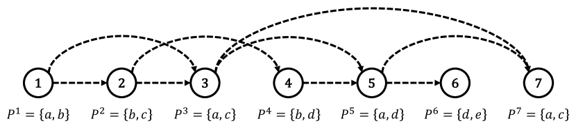
(a) Ex-ante dependence graph.

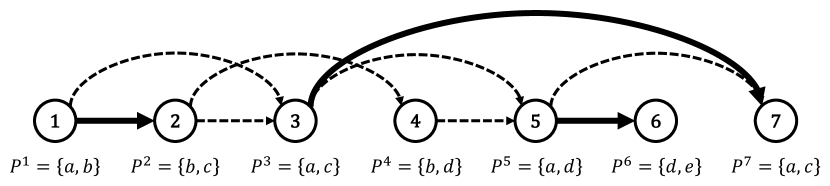
(b) Ex-post dependence graph (bold and solid edges).

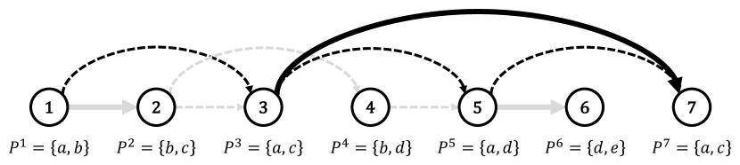
(c) Dependence subgraph associated with a fixed element $a$.

Figure 2: Example of dependence graphs with five ground elements and a sequence of seven pairs.

Each arc in the ex-ante dependence graph represents two pairs in the sequence in which the OCS could use the same random bit to select oppositely. By construction, there are at most two outgoing arcs and at most two incoming arcs for each node.

In particular, consider any arc $(j_{1},j_{2})_{i}$ in the ex-ante dependence graph, with $i$ being the common element. If the randomness used by the OCS satisfies (1) pair $j_{1}$ is a sender, (2) $i_{m}=i$ in pair $j_{1}$, (3) pair $j_{2}$ is a receiver, and (4) $i_{m}=i$ in pair $j_{2}$, the selections in the two pairs would be perfectly negatively correlated in the sense that $i$ is selected in exactly one of the two pairs. Each of these four events happens independently with probability $\nicefrac{{1}}{{2}}$. Hence, we achieve the above perfect negative correlation with probability $\nicefrac{{1}}{{16}}$.

Ex-post Dependence Graph.

The ex-post dependence graph $G^{\textrm{\em ex-post}}=(V,E^{\textrm{\em ex-post}})$ is a subgraph of the ex-ante dependence graph that keeps the arcs corresponding to pairs that are perfectly negatively correlated, given the realization of whether each step is a sender or a receiver, and the value of $m$ therein. Equivalently, the ex-post dependence graph is realized as follows. Over the randomness with which the OCS decides whether each step is a sender or a receiver, and the values of $m$, each node in the ex-ante dependence graph effectively picks at most one of its incident arcs, each with probability $\nicefrac{{1}}{{4}}$; an arc is realized in the ex-post graph if both incident nodes choose it. With this interpretation, we get that the ex-post graph is a matching. The OCS may be viewed as a randomized online algorithm that picks a matching in the ex-ante graph such that each arc in the ex-ante graph is chosen with probability lower bounded by a constant. See Figure 2(b) for an example.

Proof of Lemma 8.

Let $j_{1}<j_{2}<\dots$ be the pairs involving a ground element $i$. We will use the element $a$ and $k=4$ in Figure 2(c) as a running example, where $j_{1}=1,j_{2}=3,j_{3}=5,j_{4}=7$ and the relevant arcs in the dependence graphs are $(1,3)_{a}$, $(3,5)_{a}$, $(3,7)_{c}$, and $(5,7)_{a}$.

If at least one of the arcs among $j_{1}<j_{2}<\dots<j_{k}$ are realized in the ex-post dependence graph, element $i$ must be selected at least once. This is because the randomness (related to the choice of $\ell$ in the OCS) is perfectly negatively correlated in the two incident nodes of the arc and thus, $i$ is selected exactly once in these two steps. Importantly, this is true even if the arc is not due to element $i$. For example, given that the arc $(3,7)_{c}$ is realized in Figure 2(c), element $a$ must be selected at least once after step $7$.

On the other hand, if none of these arcs are realized, then the random bits used in the $k$ steps $j_{1}<j_{2}<\dots<j_{k}$ are independent. For example, consider element $a$ and $k=3$ in Figure 2(c). Element $a$ is selected independently with probability $\nicefrac{{1}}{{2}}$ in steps $j_{1}=1$, $j_{2}=3$, and $j_{3}=5$, given that neither $(1,3)_{a}$ nor $(3,5)_{a}$ is realized.

Importantly, even if some of these pairs are receivers in that the selections therein are based on the random bits realized earlier by some senders, from $i$’s point of view, they are still independent of the randomness in the other rounds that $i$ is involved in. For example, from $c$’s point of view in Figure 2(c), even though the selection in step $2$ is determined by the selection in step $1$, it is independent of the selections in steps $3$ and $7$, which involve $c$.

Putting this together, the probability that $i$ is never selected after steps $j_{1}<j_{2}<\dots<j_{k}$ is equal to the probability that (1) none of the arcs among these steps is realized, times the probability that (2) none of the $k$ independent random selections pick $i$. This follows from the law of total probability. The latter quantity equals $2^{-k}$, so it remains to analyze the former. We shall upper bound it by the probability that none of the arcs $(j_{1},j_{2})_{i},(j_{2},j_{3})_{i},\dots,(j_{k-1},j_{k})_{i}$ is realized. We shall omit the subscript $i$ in the rest of the proof for brevity. Denote this event as $F_{k}$ and its probability as $f_{k}$.

Trivially, we have $f_{0}=f_{1}=1$. To prove that the recurrence in Eqn. (16) governs $f_{k}$, further divide event $F_{k}$ into two subevents. Let $A_{k}$ the event that none of the arcs $(j_{1},j_{2}),(j_{2},j_{3}),\dots,(j_{k-1},j_{k})$ is realized, and node $j_{k}$ picks arc $(j_{k},j_{k+1})$ in realizing the ex-post dependence graph. Let $B_{k}$ be the event that none of the arcs is realized and node $j_{k}$ does not pick arc $(j_{k},j_{k+1})$. Let $a_{k}$ and $b_{k}$ be the probability of $A_{k}$ and $B_{k}$, respectively. We have that $A_{k}$ and $B_{k}$ form a partition of $F_{k}$, and thus:

$$f_{k}=a_{k}+b_{k}\leavevmode\nobreak\ .$$

If node $j_{k}$ picks arc $(j_{k},j_{k+1})$, which happens with probability $\nicefrac{{1}}{{4}}$, arc $(j_{k-1},j_{k})$ is not realized by definition, regardless of the remaining randomness. Therefore, conditioned on the choice of $j_{k}$, subevent $A_{k}$ happens if and only if the choices made by steps $j_{1},j_{2},\dots j_{k-1}$ is such that none of $(j_{1},j_{2}),\dots,(j_{k-2},j_{k-1})$ is realized, i.e., when $F_{k-1}$ happens. That is:

$$a_{k}=\frac{1}{4}f_{k-1}\leavevmode\nobreak\ .$$

On the other hand, if pair $j_{k}$ does not pick $(j_{k},j_{k+1})$, there are two possibilities. The first case is when $j_{k}$ picks $(j_{k-1},j_{k})$, which happens with probability $\nicefrac{{1}}{{4}}$. In this case, the choices made by $j_{1},\dots,j_{k-1}$ must be such that none of $(j_{1},j_{2}),\dots,(j_{k-2},j_{k-1})$ is realized, and $j_{k-1}$ does not pick $(j_{k-1},j_{k})$, i.e., $B_{k-1}$ happens. The second case is when $j_{k}$ picks neither $(j_{k-1},j_{k})$ nor $(j_{k},j_{k+1})$, which happens with probability $\nicefrac{{1}}{{2}}$. In this case, the choices made by $j_{1},\dots,j_{k-1}$ must be such that none of $(j_{1},j_{2}),\dots,(j_{k-2},j_{k-1})$ is realized, i.e., $F_{k-1}$ happens. Putting this together, we have:

$$b_{k}=\frac{1}{4}b_{k-1}+\frac{1}{2}f_{k-1}\leavevmode\nobreak\ .$$

Eliminating $a_{k}$’s and $b_{k}$’s with the above three equations, we get the recurrence in Eqn. (16). ∎

The same analysis generalizes to prove a stronger result, which implies a $\nicefrac{{1}}{{16}}$-OCS.

Lemma 9.

For any fixed sequence of pairs of elements, any fixed element $i$, and any disjoint collections of $k_{1},k_{2},\dots,k_{m}$ consecutive pairs involving $i$, Algorithm 2 ensures that $i$ is selected in at least one of these pairs with probability at least:

$$1-\prod_{\ell=1}^{m}2^{-k_{\ell}}\cdot f_{k_{\ell}}\leavevmode\nobreak\ .$$

Proof.

Let $j_{1}^{\ell}<j_{2}^{\ell}<\dots<j_{k_{\ell}}^{\ell}$ be the $\ell$-th subsequence of consecutive pairs involving element $i$, for any $1\leq\ell\leq m$. The probability that $i$ is never selected is equal to (1) the probability that none of the arcs among the steps in these collections is realized, times (2) the probability that all $\sum_{\ell=1}^{m}k_{\ell}$ random bits are against $i$. The latter is $\prod_{\ell=1}^{m}2^{-k_{\ell}}$. We upper bound the former with the probability that for any $1\leq\ell\leq m$, none of the arcs $(j_{1}^{\ell},j_{2}^{\ell}),\dots,(j_{k_{\ell}-1}^{\ell}j_{k_{\ell}}^{\ell})$ is realized. Finally, observe that the events are independent for different collections $\ell$ because the event concerning each collection only relies on the randomness of the nodes in the collection. Hence, it is at most $\prod_{\ell=1}^{m}f_{k_{\ell}}$. ∎

5.2 Optimizing the OCS: Proof of Theorem 3

Similar to the warmup algorithm, we will realize the ex-post dependence graph by letting each node be either a sender or a receiver independently and randomly. The probability of letting a node be a sender, denoted as $p$, will be optimized later.

A sender uses a fresh random bit to select an element from the corresponding pair. Further, it randomly picks an out-arc in the ex-post graph and sends its selection along the out-arc. Although the out-neighbors and out-arcs have yet to arrive, we can refer to them as the one due to the first and second element in the current pair, respectively. This is identical to the warmup case.

A receiver, on the other hand, adapts to the information it receives and makes the opposite selection. The improved OCS proactively checks both in-arcs of a receiver; in contrast, the warmup algorithm checks only one randomly chosen in-arc. Concretely, check both in-arcs in the ex-ante graph to see if any in-neighbor is a sender who picks the arc between them. If both in-neighbors are senders and both pick the corresponding arcs, choose one randomly. Add the arc to the ex-post dependence graph. Suppose a receiver $j$ receives the selection by a sender $j^{\prime}$ sent along arc $(j^{\prime},j)_{i}$. Then, select $i$ in round $j$ if it is not selected in round $j^{\prime}$, and vice versa.

See Algorithm 3 for a formal definition of the improved OCS.

Algorithm 3 Improved Online Correlated Selection

Parameter:

• $p$ : probability that a node is a sender.

State variables:

• $G^{\text{\em ex-ante}}=(V,E^{\text{\em ex-ante}})$ : ex-ante dependence graph; initially, $V=E^{\text{\em ex-ante}}=\emptyset$.

• $G^{\text{\em ex-post}}=(V,E^{\text{\em ex-post}})$ : ex-post dependence graph; initially, $V=E^{\text{\em ex-post}}=\emptyset$.

• $\tau_{j}\in\big{\{}\textrm{\em sender},\textrm{\em receiver}\big{\}}$ for any $j\in V$.

On receiving a pair $j$ of elements $i_{1}$ and $i_{2}$:

1. Add $j$ to $V$.

2. For $k\in\{1,2\}$, let $j_{k}$ be the last pair which involves $i_{k}$; add an arc $(j_{k},j)_{i_{k}}$ to $E^{\text{\em ex-ante}}$.

3. With probability $p$, let it be a sender:

   1. Let $i^{*}=i_{1}$ or $i_{2}$, each with probability $\nicefrac{{1}}{{2}}$.

   2. Pick an out-arc randomly.

4. Otherwise, i.e., with probability $1-p$, let it be a receiver:

   1. Pick a $j_{m}$, $m\in\{1,2\}$, that is a sender who picks arc $(j_{m},j)_{i_{m}}$ (break ties randomly):

      1. Add arc $(j_{m},j)_{i_{m}}$ to $E^{\text{\em ex-post}}$.

      2. Let $i^{*}=i_{m}$ if $i_{m}$ is not selected in round $j_{m}$, let $i^{*}=i_{-m}$ otherwise.

   2. Otherwise, let $i^{*}=i_{1}$ or $i_{2}$, each with probability $\nicefrac{{1}}{{2}}$.

5. Select $i^{*}$.

Lemma 10.

For any fixed sequence of pairs of elements, any fixed element $i$, and any disjoint subsequences of $k_{1},k_{2},\dots,k_{m}$ consecutive pairs involving $i$, Algorithm 3 ensures that $i$ is selected in at least one of these pairs with probability at least:

$$1-\prod_{\ell=1}^{m}2^{-k_{\ell}}\cdot g_{k_{\ell}}\leavevmode\nobreak\ ,$$

where $g_{k}$ is defined recursively as follows:

$$g_{k}=\begin{cases}1&\text{if $k=0,1$}\leavevmode\nobreak\ ;\\ g_{k-1}-\frac{1}{8}p\left(1-p\right)\left(4-p\right)\cdot g_{k-2}&\text{if $k\geq 2$}\leavevmode\nobreak\ .\end{cases}$$ (17)

Corollary 11.

Algorithm 3 is a $\frac{1}{8}p(1-p)(4-p)$-OCS.

To prove Theorem 3, let $p=\frac{5-\sqrt{13}}{3}$ to maximize $\frac{1}{8}p\big{(}1-p\big{)}\big{(}4-p\big{)}=\frac{13\sqrt{13}-35}{108}>0.1099$.

Proof of Lemma 10

Let $j^{\ell}_{1}<j^{\ell}_{2}<\dots<j^{\ell}_{k_{\ell}}$, $1\leq\ell\leq m$, be the subsequences of consecutive pairs that involve element $i$. The algorithm uses two kinds of independent random bits. The first kind is used to realized the ex-post dependence graph, i.e., the random type of each pair, the random out-arc chosen by each sender, and the random in-neighbor of each receiver in the tie-breaking case. The second kind is the random selections by senders, and by receivers that fail to receive the selection of any sender. Importantly, the two kinds of randomness are independent.

Similar to the warmup case, we are interested in the event that there is no arc among these pairs in the ex-post dependence graph:

$$F=\left\{\textrm{nodes $j^{\ell}_{s}$, for $1\leq\ell\leq m$ and $1\leq s\leq k_{\ell}$, are disjoint in $G^{\text{\em ex-post}}$}\right\}\leavevmode\nobreak\ .$$

If there is an arc between two pairs in the collections in the ex-post dependence graph, $i$ is selected in exactly one of the two pairs. Otherwise, the selections in these pairs are independent. Hence, the probability that $i$ is never selected is equal to the product of (1) the probability that the $\sum_{\ell=1}^{m}k_{\ell}$ nodes in the collections are disjoint in the ex-post dependence graph, and (2) none of the $\sum_{\ell=1}^{m}k_{\ell}$ independent random selections picks $i$. This follows from the law of total probability. The former quantity is $\Pr(F)$, and the latter is equal to $2^{-\sum_{\ell=1}^{m}k_{\ell}}$. Putting this together, it equals:

$$2^{-\sum_{1\leq\ell\leq m}k_{\ell}}\cdot\Pr(F)\leavevmode\nobreak\ .$$

Therefore, it remains to show that:

$$\Pr(F)\leq\prod_{\ell=1}^{m}g_{k_{\ell}}\leavevmode\nobreak\ .$$ (18)

Which arcs are we concerned about in the event $F$? Since these are subsequences of consecutive pairs involving element $i$, the arcs of the form $(j^{\ell}_{s},j^{\ell}_{s+1})_{i}$ always exist in the ex-ante dependence graph. To characterize whether some of these arcs are realized in the ex-post graphs, we need to further consider another set of arcs as follows.

For any $1\leq\ell\leq m$, consider the in-arcs of nodes $j^{\ell}_{1}<\dots<j^{\ell}_{k_{\ell}}$ in the ex-ante dependence graph due to the element other than $i$. Let them be $(\hat{j}^{\ell}_{s},j^{\ell}_{s})$, for $1\leq s\leq k_{\ell}$. We omit the subscript that denotes the common element in the two nodes, with the understanding that they are due to the element other than $i$ in the round of $j^{\ell}_{s}$. Then, an arc $(j^{\ell}_{s},j^{\ell}_{s+1})_{i}$ is realized in the ex-post graph if:

1. Node $j^{\ell}_{s}$ is a sender that picks arc $(j^{\ell}_{s},j^{\ell}_{s+1})_{i}$;

2. Node $j^{\ell}_{s+1}$ is a receiver;

3. Either node $\hat{j}^{\ell}_{s+1}$ is a receiver, or it is a sender but does not choose arc $(\hat{j}^{\ell}_{s+1},j^{\ell}_{s+1})$, or the tie-breaking by node $j^{\ell}_{s+1}$ is in favor of $j^{\ell}_{s}$.

Binding Case.

First, suppose all $\hat{j}^{\ell}_{s}$’s exist, and the $j^{\ell}_{s}$’s and $\hat{j}^{\ell}_{s}$’s are all distinct. It is relatively easy to analyze because in this case it suffices to consider arcs of the form $(j^{\ell}_{s},j^{\ell}_{s+1})_{i}$, and different subsequences of consecutive pairs depend on disjoint sets of random bits and therefore may be analyze separately. This turns out to be the binding case of the analysis. We will analyze the binding case in Lemma 12 and show in Lemma 13 that this is the worst-case scenario that maximizes $\Pr(F)$.

Lemma 12.

In the binding case, the probability of event $F$ is:

$$\Pr(F)=\prod_{\ell=1}^{m}g_{k_{\ell}}\leavevmode\nobreak\ .$$

Proof.

We start by formalizing the aforementioned implications of the assumption that all $j^{\ell}_{s}$’s and $\hat{j}^{\ell}_{s}$’s are distinct. First, two pairs in the collections are connected if and only if they are consecutive pairs in the same collection, e.g., $j^{\ell}_{s-1}$ and $j^{\ell}_{s}$, and arc $(j^{\ell}_{s-1},j^{\ell}_{s})_{i}$ is realized. A pair $j^{\ell}_{s}$ with $s>1$ cannot be the receiver of a sender other than $j^{\ell}_{s-1}$ in the collections because $\hat{j}^{\ell}_{s}$’s are not in the collections by the assumption. Second, the realization of these arcs in different collections are independent. The realization of arcs of the form $(j^{\ell}_{s-1},j^{\ell}_{s})_{i}$, for any fixed collection $\ell$, depends only on the realization of first kind of randomness related to nodes with superscript $\ell$, i.e., $j^{\ell}_{s}$’s and $\hat{j}^{\ell}_{s}$’s.

Next, we focus on a fixed subsequence $\ell$ and analyze the probability that no arc of the form $(j^{\ell}_{s},j^{\ell}_{s+1})_{i}$, for $1\leq s<k_{\ell}$, is realized. To simplify notation, we omit the superscripts and subscripts $\ell$ and write $j_{1}<j_{2}<\dots<j_{k}$ and $\hat{j}_{2},\hat{j}_{3},\dots,\hat{j}_{k}$. Let $G_{k}$ denote this event and $g_{k}$ be its probability. Trivially, we have $g_{0}=g_{1}=1$. It remains to show that $g_{k}$ follows the recurrence in Eqn. (17).

We will do so by further considering an auxiliary subevent $A_{k}$, which requires not only $G_{k}$ to happen, but also $j_{k}$ to be a sender who picks the out-arc due to $i$. Let $a_{k}$ denote its probability.

Auxiliary Event.

If $j_{k}$ is a sender who picks the out-arc due to $i$, which happens with probability $\nicefrac{{p}}{{2}}$, arc $(j_{k-1},j_{k})_{i}$ would not be realized regardless of the randomness of the other nodes in the collection. Therefore, under this condition, event $A_{k}$ reduces to event $G_{k-1}$.

$$a_{k}=\frac{p}{2}\cdot g_{k-1}\leavevmode\nobreak\ .$$

Main Event.

If $j_{k}$ is a sender, which happens with probability $p$, arc $(j_{k-1},j_{k})_{i}$ would not be realized regardless of the randomness of the other nodes in the collection. Therefore, under this condition, event $G_{k}$ reduces to event $G_{k-1}$. The contribution of this part to the probability of $G_{k}$ is:

$$p\cdot g_{k-1}\leavevmode\nobreak\ .$$

If $j_{k}$ is a receiver (probability $1-p$), but $\hat{j}_{k}$ is a sender who picks arc $(\hat{j}_{k},j_{k})$ (probability $\nicefrac{{p}}{{2}}$), and the tie-breaking at $j_{k}$ is in favor of $\hat{j}_{k}$ (probability $\nicefrac{{1}}{{2}}$), we still have that arc $(j_{k-1},j_{k})_{i}$ cannot be realized regardless of the randomness of the other nodes. The contribution of this part to the probability of $G_{k}$ is:

$$\frac{p(1-p)}{4}g_{k-1}\leavevmode\nobreak\ .$$

Otherwise, $j_{k-1}$ must not be a sender who picks arc $(j_{k-1},j_{k})_{i}$, or else arc $(j_{k-1},j_{k})_{i}$ would be realized. Therefore, conditioned on being in this case, events $G_{k}$ reduces to event $G_{k-1}\setminus A_{k-1}$. The contribution of this part to the probability of $G_{k}$ is:

$$(1-p)(1-\frac{p}{4})\left(g_{k-1}-a_{k-1}\right)\leavevmode\nobreak\ .$$

Putting everything together, we have:

$$g_{k}=g_{k-1}-(1-p)\left(1-\frac{p}{4}\right)a_{k-1}\leavevmode\nobreak\ .$$

Eliminating $a_{k}$’s by combining the two equations, we get the recurrence in Eqn. (17). ∎

Lemma 13.

The probability of event $F$ is maximized in the binding case.

Proof.

Here are the possible violations of the conditions of the regular case:

1. Some arc $(\hat{j}^{\ell}_{s},j^{\ell}_{s})$ may not exist, i.e., the element other than $i$ in pair $j^{\ell}_{s}$ has its first appearance in pair $j^{\ell}_{s}$.

2. There may be $\ell,\ell^{\prime},s,s^{\prime}$ such that $\hat{j}^{\ell}_{s}=j^{\ell^{\prime}}_{s^{\prime}}$, i.e., the element other than $i$ in pair $j^{\ell}_{s}$ is also a element in pair $j^{\ell^{\prime}}_{s^{\prime}}$, and in no other pairs in between.

3. There may be $\ell,\ell^{\prime},s,s^{\prime}$ such that $\hat{j}^{\ell}_{s}=\hat{j}^{\ell^{\prime}}_{s^{\prime}}$.

We use a coupling argument to compare the probability of event $F$ in a general case, potentially with some of the above violations, with the probability in the binding case.

Type-1 Violation.

Consider an instance almost identical to the one at hand, except we introduce a new node $\hat{j}_{s}^{\ell}$ for such a violation. For example, let pair $\hat{j}_{s}^{\ell}$ be at the beginning of the sequence, and let it contain the element other than $i$ in pair $j_{s}^{\ell}$ and a new dummy element that does not appear elsewhere. Further, couple the two instances by letting the common nodes realize identical random bits, and letting the new node draw fresh random bits. We claim that whenever event $F$ happens in the original instance, it also happens in the new instance. If arc $(\hat{j}_{s}^{\ell},j_{s}^{\ell})$ is not realized, the rest of the arcs are realized identically in the two cases. Otherwise, having arc $(\hat{j}_{s}^{\ell},j_{s}^{\ell})$ may preclude arc $(j_{s-1}^{\ell},j_{s}^{\ell})_{i}$ from being realized, making event $F$ more likely to happen in the new instance.

Type-2 Violation.

Consider an instance almost identical to the one at hand, except we introduce a new node $\hat{j}_{s}^{\ell}\neq j_{s^{\prime}}^{\ell^{\prime}}$ for such a violation. For example, let $\hat{j}_{s}^{\ell}$ be a pair arriving after $j_{s^{\prime}}^{\ell^{\prime}}$ and before $j_{s}^{\ell}$ which involves the element other than $i$ in these two pairs and a new dummy element that does not appear elsewhere. Further, couple the two instances by letting the common nodes realize identical random bits, and letting the new nodes draw fresh random bits. We claim that whenever event $F$ happens in the original instance, it also happens in the new instance. Since $F$ happens in the original instance, arc $(j_{s^{\prime}}^{\ell^{\prime}},j_{s}^{\ell})$ is not realized. If further arc $(\hat{j}_{s}^{\ell},j_{s}^{\ell})$ is not realized, the rest of the arcs are realized identically in the two cases. Otherwise, having arc $(\hat{j}_{s}^{\ell},j_{s}^{\ell})$ may preclude arc $(j_{s-1}^{\ell},j_{s}^{\ell})_{i}$ from being realized, making event $F$ more likely to happen in the new instance.

Type-3 Violation.

Consider an instance almost identical to the one at hand, except we introduce a new node $\hat{j}_{s}^{\ell}\neq\hat{j}_{s^{\prime}}^{\ell^{\prime}}$ for such a violation. For example, let $\hat{j}_{s}^{\ell}$ be a pair arriving right before $j_{s}^{\ell}$ which involves the element other than $i$ in pair $j_{s}^{\ell}$ and a new dummy element that does not appear elsewhere. To avoid confusion in the following discussion, let $\hat{j}$ be the node in the type-3 violation the original instance, and let $\hat{j}_{s}^{\ell}\neq\hat{j}_{s^{\prime}}^{\ell^{\prime}}$ be the nodes in the new instance. Further, couple the two instances by letting nodes other than $\hat{j}$, $\hat{j}_{s}^{\ell}$, and $\hat{j}_{s^{\prime}}^{\ell^{\prime}}$ realize identical random bits. To define the coupling for these three nodes, we need some notations. We say that node $j_{s}^{\ell}$ needs help if node $j_{s-1}^{\ell}$ is a sender who picks arc $(j_{s-1}^{\ell},j_{s}^{\ell})_{i}$, and if node $j_{s}^{\ell}$ is a receiver who breaks tie against $j_{s-1}^{\ell}$. For $F$ to happens in this case, $\hat{j}_{s}^{\ell}$ must be a sender who picks arc $(\hat{j}_{s}^{\ell},j_{s}^{\ell})$. Define similarly for node $j_{s^{\prime}}^{\ell^{\prime}}$. If $j_{s}^{\ell}$ needs help but $j_{s^{\prime}}^{\ell^{\prime}}$ does not, let $j^{*}$ and $j_{s}^{\ell}$ realize identical random bits, and let $\hat{j}_{s^{\prime}}^{\ell^{\prime}}$ draw fresh random bits; and vice versa. Otherwise, i.e., if none or both of them need help, let them have independent random bits. Then, when at most one of them needs help, event $F$ happens in the original instance if and only if it happens in the new instance, since the realization of the relevant arcs are identical. If both need help, on the other hand, $F$ cannot happen in the original instance because at least one of $(j_{s-1}^{\ell},j_{s}^{\ell})_{i}$ or $(j_{s^{\prime}-1}^{\ell^{\prime}},j_{s^{\prime}}^{\ell^{\prime}})_{i}$ would be realized. ∎

6 Conclusion

This paper presents an online primal-dual algorithm for the edge-weighted bipartite matching problem that is $0.5086$-competitive, resolving a long-standing open problem in the study of online algorithms. In particular, this work merges and refines the results of Fahrbach and Zadimoghaddam [11] and Huang and Tao [18, 20] to give a simpler algorithm under the online primal-dual framework. Our work initiates the study of online correlated selection, a key algorithmic ingredient that quantifies the level of negative correlation in online assignment problems, and we believe this technique will find further applications in other online problems.

Using independent random bits to make selections yields a $0$-OCS (no negative correlation), and using an imaginary $1$-OCS with perfect negative correlation results in inconsistent assignments. Therefore, we aim to design an online matching algorithm that uses partial negative correlation. We start by constructing a $\nicefrac{{1}}{{16}}$-OCS, and then we optimize this subroutine to obtain a $0.109927$-OCS. Designing a $\gamma$-OCS with the largest possible $\gamma\in[0,1]$ is an interesting open problem on its own, and would directly lead to an improved competitive ratio for the edge-weighted online bipartite matching problem. However, even if a 1-OCS existed, the best competitive ratio that can be achieved using this approach is at most $\nicefrac{{5}}{{9}}$, as shown in Appendix B. Thus, we need fundamentally new ideas in order to come closer to the optimal $1-\nicefrac{{1}}{{e}}$ ratio in the unweighted and vertex-weighted cases. One potential approach is to consider an OCS that allows for more than two candidates in each round, which we call a multiway OCS. We leave this as another interesting open problem for future works.

Appendix A Unweighted Online Matching

This section shows that the two-choice greedy algorithm is strictly better than $\nicefrac{{1}}{{2}}$-competitive when combined with an OCS in the randomized rounds to ensure partial negative correlation.

Theorem 14.

The two-choice greedy algorithm with the randomized rounds that use a $0.1099$-OCS is at least $0.508$-competitive for unweighted online bipartite matching.

Proof.

In the unweighted case, it suffices to consider a single weight-level $w=1$. Thus, for each offline vertex $i$, we write $k_{i}=k_{i}(1)$ for brevity. We will maintain $\bar{x}_{i}=1-2^{-k_{i}}\cdot g_{k_{i}}$ for each offline vertex $i$, which according to Lemma 10 lower bounds the probability that $i$ is matched. Correspondingly, we maintain the following lower bound on the primal objective:

$$\bar{\textsc{P}}=\sum_{i\in L}\bar{x}_{i}\leavevmode\nobreak\ .$$

To prove the stated competitive ratio, it suffices to explain how to maintain a dual assignment such that (1) the dual objective equals the lower bound of the primal objective, i.e., $\textsc{D}=\bar{\textsc{P}}$, and (2) it is approximately feasible up to a $\Gamma$ factor, i.e., $\alpha_{i}+\beta_{j}\geq\Gamma$ for every edge $(i,j)\in E$.

Dual Updates

The dual updates are based on a solution to a finite version of the following LP. All of the solution values are presented in Table 2 at the end of this section. The constraints below are simpler than in the more general edge-weighted case, but the competitive ratio we achieve is almost the same. Note in this LP that $\Delta\alpha(k)=\alpha(k+1)-\alpha(k)$ denotes the forward difference operator.

Lemma 15.

The optimal value of the LP below is at least $0.508$:

maximize $$\Gamma$$

subject to $$\Delta\alpha(k)+\Delta\beta(k)\leq 2^{-k}\cdot g_{k}-2^{-k-1}\cdot g_{k+1} \forall k\geq 0$$ (19)

$$\sum_{\ell=0}^{k-1}\Delta\alpha(\ell)+2\cdot\Delta\beta(k)\geq\Gamma \forall k\geq 0$$ (20)

$$\Delta\beta(k)\geq\Delta\beta(k+1) \forall k\geq 0$$ (21)

$$\Delta\alpha(k),\Delta\beta(k)\geq 0 \forall k\geq 0$$

Consider an online vertex $j\in R$, and recall that $k_{\min}=\min_{i\in N(j)}k_{i}$ denotes the minimum value of $k_{i}$ among offline neighbors $i$ of vertex $j$. First suppose it is a randomized round. Recall that $i_{1}$ and $i_{2}$ denote the two candidate offline vertices shortlisted in round $j$. Then, we have $k_{i}=k_{\min}$ for both $i\in\{i_{1},i_{2}\}$. Note in the unweighted case that the algorithm would enter a deterministic round if there is a unique offline vertex with minimum $k_{i}$. In the primal, $\bar{x}_{i}$ increases by $2^{-k_{\min}}\cdot g_{k_{\min}}-2^{-k_{\min}-1}\cdot g_{k_{\min}+1}$ for both $i\in\{i_{1},i_{2}\}$. In the dual, increase $\alpha_{i}$ by $\Delta\alpha(k_{\min})$ for both $i\in\{i_{1},i_{2}\}$, and let $\beta_{j}=2\cdot\Delta\beta(k_{\min})$ where each $i\in\{i_{1},i_{2}\}$ contributes $\Delta\beta(k_{\min})$.

Next, suppose it is a deterministic round. Recall that $i^{*}$ denotes the offline vertex to which vertex $j$ is matched deterministically. Then, $x_{i^{*}}$ increases by $2^{-k_{\min}}\cdot g_{k_{\min}}$ in the primal. In the dual, increase $\alpha_{i^{*}}$ by $\sum_{\ell\geq k_{\min}}\Delta\alpha(\ell)$, and let $\beta_{j}=2\cdot\Delta\beta(k_{\min}+1)$. No update is needed in an unmatched round, as $\bar{\textsc{P}}$ remains the same.

Objective Comparisons

Next, we show that the increment in the dual objective D is at most that in the lower bound of primal objective, i.e., $\bar{\textsc{P}}$. In a randomized round, it follows by Eqn. (19). In a deterministic round, it follows by a sequence of inequalities below:

$$\sum_{\ell\geq k}\Delta\alpha(\ell)+2\cdot\Delta\beta(k+1) \leq\sum_{\ell\geq k}\Delta\alpha(\ell)+\Delta\beta(k)+\Delta\beta(k+1)$$ (Eqn. (21))

$$\leq\sum_{\ell\geq k}\big{(}\Delta\alpha(\ell)+\Delta\beta(\ell)\big{)}$$

$$\leq\sum_{\ell\geq k}\big{(}2^{-\ell}\cdot g_{\ell}-2^{-\ell-1}\cdot g_{\ell+1}\big{)}$$ (Eqn. (19))

$$=2^{-k}\cdot g_{k}\leavevmode\nobreak\ .$$

Approximate Dual Feasibility.

We first summarize the following invariants, which follow by the definition of the dual updates.

• For any offline vertex $i\in L$, $\alpha_{i}=\sum_{\ell=0}^{k_{i}-1}\Delta\alpha(\ell)$.

• For any online vertex $j$, $\beta_{j}=2\cdot\Delta\beta(k)$ if it is matched either in a randomized round to neighbors with $k_{i}=k$, or in a deterministic round to a neighbor with $k_{i}=k-1$.

For any edge $(i,j)\in E$, consider the value of $k_{i}$ at the time when $j$ arrives. If $k_{i}=\infty$, the value of $\alpha_{i}$ alone ensures approximately dual feasibility because:

$$\alpha_{i} =\sum_{\ell\geq 0}\Delta\alpha(\ell)$$

$$=\lim_{k\to\infty}\sum_{\ell=0}^{k-1}\Delta\alpha(\ell)$$

$$\geq\Gamma-\lim_{k\to\infty}\beta(k)$$ (Eqn. (20))

$$=\Gamma\leavevmode\nobreak\ . 0$$ (Eqn. (19), whose RHS tends to )

Otherwise, by the definition of the two-choice greedy algorithm, $j$ is either matched in a randomized round to two vertices with $k_{i^{\prime}}\leq k_{i}$, or in a deterministic round to a vertex with $k_{i^{\prime}}<k_{i}$. In both cases, we have:

$$\beta_{j}\geq 2\cdot\Delta\beta(k_{i})\leavevmode\nobreak\ .$$

Approximate dual feasibility now follows by $\alpha_{i}=\sum_{\ell=0}^{k_{i}-1}\Delta\alpha(\ell)$ and Eqn. (20). ∎

Proof of Lemma 15.

Consider a restricted version of the LP which is finite. For some positive $k_{\max}$, let $\Delta\alpha(k)=\Delta\beta(k)=0$ for all $k>k_{\max}$. Then, the linear program becomes:

maximize $$\Gamma$$

subject to $$\Delta\alpha(k)+\Delta\beta(k)\leq 2^{-k}\cdot g_{k}-2^{-k-1}\cdot g_{k+1} 0\leq k\leq k_{\max}$$

$$\sum_{\ell=0}^{k-1}\Delta\alpha(\ell)+2\cdot\Delta\beta(k)\geq\Gamma 0\leq k\leq k_{\max}$$

$$\sum_{\ell=0}^{k_{\max}}\Delta\alpha(\ell)\geq\Gamma$$

$$\beta(k)\geq\beta(k+1) 0\leq k<k_{\max}$$

$$\Delta\alpha(k),\beta(k)\geq 0 0\leq k\leq k_{\max}$$

See Table 2 for an approximately optimal solution for the restricted LP with $k_{\max}=8$, which gives a competitive ratio of $\Gamma\approx 0.508986$. ∎

$k$	$g_{k}$	$\Delta\alpha(k)$	$\beta(k)$
$0$	$1.00000000$	$0.24550678$	$0.25449322$
$1$	$1.00000000$	$0.14574204$	$0.13173982$
$2$	$0.89007253$	$0.06613120$	$0.05886880$
$3$	$0.78014506$	$0.02907108$	$0.02580320$
$4$	$0.68230164$	$0.01273424$	$0.01126766$
$5$	$0.59654227$	$0.00559236$	$0.00490054$
$6$	$0.52153858$	$0.00248248$	$0.00210436$
$7$	$0.45596220$	$0.00114193$	$0.00086312$
$8$	$0.39863078$	$0.00058431$	$0.00029216$

Table 2: An approximately optimal solution to the factor-revealing linear program with $k_{\max}=8$ in the unweighted case. The competitive ratio obtained is $\Gamma\approx 0.508986$.

Appendix B Hard Instances

This section presents two families of unweighted graphs that demonstrate some hardness results for the online matching algorithms considered in this paper.

B.1 Upper Triangular Graphs

Consider a bipartite graph with $n$ vertices on each side. Let each online vertex $1\leq j\leq n$ be incident to the offline vertices $j\leq i\leq n$. Thus, the adjacency matrix (with online vertices as rows and offline vertices as columns) is an upper triangular matrix. This is a standard instance for showing hardness that dates back to Karp et al. [27].

Theorem 16.

The two-choice greedy algorithm using independent random bits in different randomized rounds is only $(\nicefrac{{1}}{{2}}+o(1))$-competitive.

Proof.

For ease of presentation, suppose the algorithm chooses candidates in reverse lexicographical order. Consider an upper triangular graph with $n=3^{k}$ for some large positive integer $k$. First, observe that there is a perfect matching where the $i$-th online vertex is matched to the $i$-th offline vertex. Hence, the optimal value is $n$.

Next, consider the performance of the online algorithm. The first $\nicefrac{{n}}{{3}}=3^{k-1}$ vertices are matched to the last $\nicefrac{{2}}{{3}}$ fraction of the offline vertices in randomized rounds. That is, their correct neighbors in the perfect matching are left unmatched, while the other offline vertices are only half matched. Then, the first one third of the remaining online vertices (i.e., $\nicefrac{{1}}{{3}}\cdot\nicefrac{{2n}}{{3}}=2\cdot 3^{k-2}$ of them in total) are matched to the last $(\nicefrac{{2}}{{3}})^{2}$ fraction of the offline vertices in randomized rounds. That is, their correct neighbors in the perfect matching are left matched by only half, while the correct neighbors of subsequent online vertices are now matched by three quarters. The argument goes on recursively.

Therefore, omitting a lower order term due to the last $2^{k}=n^{\log_{3}2}$ vertices on both sides, the expected size of the matching is:

$$\left(1\cdot\frac{1}{3}+\frac{1}{2}\cdot\frac{2}{9}+\cdots+\left(\frac{1}{2}\right)^{k}\cdot\frac{2^{k}}{3^{k+1}}+\cdots\right)n =\left(\frac{1}{3}+\frac{1}{9}+\cdots+\frac{1}{3^{k+1}}+\cdots\right)n$$

$$=\frac{n}{2}\leavevmode\nobreak\ .$$

Hence, the two-choice greedy algorithm is at best $(\nicefrac{{1}}{{2}}+o(1))$-competitive. ∎

Theorem 17.

The imaginary two-choice greedy algorithm with perfect negative correlation across different randomized rounds is only $\nicefrac{{5}}{{9}}$-competitive.

Proof.

For ease of presentation, suppose the algorithm chooses candidates in reverse lexicographical order. Consider an upper triangular graph with $n=9$. There are nine vertices on each side, denoted as $i_{1},i_{2},\dots,i_{9}$ and $j_{1},j_{2},\dots,j_{9}$, and a perfect matching with $i_{k}$ matched to $j_{k}$ for $k=1,2,\dots,9$. The first three online vertices, $j_{1}$, $j_{2}$, and $j_{3}$, are connected to all offline vertices. After their arrivals, $i_{1}$, $i_{2}$, and $i_{3}$ are unmatched while the remaining six offline vertices are matched by half. Then, the next two online vertices, $j_{4}$ and $j_{5}$, are connected to the last six offline vertices, i.e., $j_{4}$ to $j_{9}$. After their arrival, $i_{4}$ and $i_{5}$ remain matched by half, while $i_{6}$ to $i_{9}$ are fully matched. Therefore, the algorithm finds a matching of size $\nicefrac{{1}}{{2}}\cdot 2+1\cdot 4=5$ in expectation, but the optimal matching has size $9$. The competitive ratio is $\nicefrac{{5}}{{9}}$, which matches the lower bound that we want to show. ∎

B.2 Erdös–Rényi Upper Triangular Graphs

Consider the following random bipartite graph that has $n$ vertices on each side. Each online vertex $1\leq j\leq n$ is incident to the offline vertex $i=j$ with certainty, and each offline vertex $j<i\leq n$ is adjacent to $j$ independently with probability $p$, where $0<p<1$ is a parameter to be determined.

By considering the Erdös–Rényi variant of upper triangular graphs instead of the original ones, we ensure that with high probability any fixed online vertex is paired with different offline vertices in its randomized round. This is effectively the worst-case scenario in the analysis of the OCS algorithm in Section 5. Letting $n=2^{13}$ and $p=2^{-6}$, an empirical evaluation shows that our analysis for the combination of a two-choice greedy algorithm and with an OCS is nearly optimal.

Theorem 18.

The competitive ratio of the two-choice greedy algorithm with the OCS in Algorithm 2 is at most $0.5057$-competitive.

Theorem 19.

The competitive ratio of the two-choice greedy algorithm with the OCS in Algorithm 3 is at most $0.51$-competitive.

Appendix C Connections to the Original Algorithm

This section explains the connections between the online primal-dual algorithm in this paper to the original algorithm by Fahrbach and Zadimoghaddam [11]. We start by briefly describing the algorithm in Algorithm 4, with minor modifications to make it consistent with the notations in this paper. Next, we simplify the algorithm by considering the special case of unweighted online matching and present the result as Algorithm 5. Finally, we explain how Algorithm 5 in the unweighted case is effectively a two-choice greedy algorithm that implicitly uses the warmup $\nicefrac{{1}}{{16}}$-OCS from Section 5.

C.1 Original Algorithm

The algorithm uses two parameters $\varepsilon,\delta>0$ that are later optimized in the analysis in [11]. These parameters are not necessary for explaining the connections between the two algorithms, so we omit their values. For each offline vertex $i\in L$, it maintains the following state variables that express the behavior of the last randomized round involving $i$. First, it maintains a boolean variable $\textsf{active}(i)$ that indicates whether the realization of the last randomized selection involving vertex $i$ can be adaptively used in the next randomized round in which $i$ is involved. The goal here is to introduce negative correlation in the same way that the $\nicefrac{{1}}{{16}}$-OCS does. Each offline vertex also maintains two state variables about the last randomized selection involving $i$: the corresponding online vertex $\textsf{index}(i)$, and the other offline vertex $\textsf{partner}(i)$ in the last randomized round. Finally, the realization of the last randomized selection is stored as $\textsf{priority}(i)$. Informally in the notation of this paper, $\textsf{priority}(i)=0$ corresponds to the case when the last randomized round involving $i$ is a receiver; otherwise (i.e., the sender case) $\textsf{priority}(i)$ is $1$ if $i$ is selected the last time, and is $2$ if $i$ is not selected.

Algorithm 4 Original $0.501$-competitive algorithm for edge-weighted bipartite matching in [11].

parameters:  $\varepsilon$, $\delta$

state variables:  $\forall i\in L$, $\textsf{active}(i)\leftarrow\textsf{false}$, $\textsf{index}(i)\leftarrow 0$, $\textsf{partner}(i)\leftarrow 0$, $\textsf{priority}(i)\leftarrow 0$, $S(i)\leftarrow 0$

for all online vertex $j$ do

   $M_{j}\leftarrow\max_{i\in L}\mathbb{E}[\textsf{gain}_{ij}]=\int_{0}^{w_{ij}}\big{(}1-y_{i}(w)\big{)}dw$

   for all offline vertices $j$ do

      if $\textsf{active}(i)=\textsf{true}$ and $w_{ij}\geq w_{i,\textsf{index}(i)}-\delta M_{j}$ then

         $\textsf{adaptive\_gain}_{ij}\leftarrow(\mathbb{E}[\textsf{gain}_{i,\textsf{index}(i)}]/3-(w_{i,\textsf{index}(i)}-w_{ij})^{+}/3-S(i))^{+}/12$ 

      else

         $\textsf{adaptive\_gain}_{ij}\leftarrow 0$

      end if

   end for

   $B\leftarrow\{i\in L:w_{ij}\geq w_{i,\textsf{index}(i)}-\delta M_{j}\text{ and }\mathbb{E}[\textsf{gain}_{ij}]+\nicefrac{{2}}{{3}}\cdot\textsf{adaptive\_gain}_{ij}\geq(1-\varepsilon)M_{j}\}$ 

   if $|B|\geq 2$ then (case 1: there are enough candidates to exploit adaptivity)

      pick $i_{1},i_{2}\in B$ with the largest $\mathbb{E}[\textsf{gain}_{ij}]+2/3\cdot\textsf{adaptive\_gain}_{ij}$ 

      set $\textsf{active}(\textsf{partner}(i))\leftarrow\textsf{false}$ for $i=i_{1},i_{2}$ 

      set $\textsf{active}(i)\leftarrow\textsf{true}$, $S(i)\leftarrow 0$, $\textsf{index}(i)\leftarrow j$ for $i=i_{1},i_{2}$ 

      set $\textsf{partner}(i_{1})\leftarrow i_{2}$ and $\textsf{partner}(i_{2})\leftarrow i_{1}$ 

      pick $\ell\in\{1,2\}$ with the larger $\textsf{adaptive\_gain}_{i_{\ell}j}$ and let $-\ell$ denote $3-\ell$ 

      draw $R\in[0,1)$ uniformly at random 

      if $R\in[0,\nicefrac{{1}}{{3}})$ or $\textsf{adaptive\_gain}_{i_{\ell}j}=0$ then

         if $\textsf{priority}_{i_{\ell}}=2$ and $\textsf{adaptive\_gain}_{i_{\ell}j}>0$ then match $j$ to $i_{\ell}$ 

         if $\textsf{priority}_{i_{\ell}}=1$ and $\textsf{adaptive\_gain}_{i_{\ell}j}>0$ then match $j$ to $i_{-\ell}$ 

         if $\textsf{priority}_{i_{\ell}}=0$ or $\textsf{adaptive\_gain}_{i_{\ell}j}=0$ then match $j$ to $i_{1}$ or $i_{2}$ with equal probability

         set $\textsf{priority}_{i_{1}}\leftarrow 0$ and $\textsf{priority}_{i_{2}}\leftarrow 0$ 

      else

         if $R\in[\nicefrac{{1}}{{3}},\nicefrac{{2}}{{3}})$ then assign $i$ to $i_{1}$ and set $\textsf{priority}_{i_{1}}\leftarrow 1$, $\textsf{priority}_{i_{2}}\leftarrow 2$

         if $R\in[\nicefrac{{2}}{{3}},1)$ then assign $i$ to $i_{2}$ and set $\textsf{priority}_{i_{1}}\leftarrow 2$, $\textsf{priority}_{i_{2}}\leftarrow 1$

      end if

   else (case 2: there is no adaptivity)

      $B^{\prime}\leftarrow\{i\in L:(w_{ij}\geq w_{i,\textsf{index}(i)}-\delta M_{j})\textnormal{ and }(\mathbb{E}[\textsf{gain}_{ij}]\geq(1-\varepsilon)M_{j})\}$ 

      $C\leftarrow\{i\in L:(w_{ij}<w_{i,\textsf{index}(i)}-\delta M_{j})\textnormal{ and }(\mathbb{E}[\textsf{gain}_{ij}]\geq(1-\varepsilon)M_{j})\}$ 

      if $|B^{\prime}\cup C|=1$ then

         match $j$ to $i_{1}\leftarrow\arg\max_{i\in L}\mathbb{E}[\textsf{gain}_{ij}]$ 

         set $S(i_{1})\leftarrow S(i_{1})+M_{j}$ 

      else

         if $B^{\prime}\neq\emptyset$ then

            $i_{1}\leftarrow$ the only advertiser in $B^{\prime}$

         else

            $i_{1}\leftarrow\arg\max_{i\in C}\mathbb{E}[\textsf{gain}_{ij}]$

         end if

         $i_{2}\leftarrow\arg\max_{i\in C\setminus\{i_{1}\}}\mathbb{E}[\textsf{gain}_{ij}]$ 

         match $j$ to $i_{1}$ or $i_{2}$ with equal probability 

         set $S(i_{1})\leftarrow S(i_{1})+M_{j}/2$ and $S(i_{2})\leftarrow S(i_{2})+M_{j}/2$

      end if

   end if

end for

For each online vertex $j\in R$, the matching decision is made using two different quality measures for the offline vertices. For each offline vertex $i$, $\textsf{gain}_{ij}$ denotes how much $i$’s heaviest edge weight would increase, should $j$ be matched to $i$. The first measure is the expectation of $\textsf{gain}_{ij}$, which equals $\int_{0}^{w_{ij}}(1-y_{i}(w))dw$ in the CCDF viewpoint of this paper. It also defines $\textsf{adaptive\_gain}_{ij}$, which captures the extra value of matching $j$ to $i$ due to the ability to make adaptive decisions based on the realization of the last randomized round involving $i$. Informally, this corresponds to the benefit of using the OCS for negative correlation in our primal-dual algorithm. The formula of $\textsf{adaptive\_gain}_{ij}$ is derived from the analysis in [11] and its interpretation is not necessary for understanding the connections between the two algorithms. We refer the reader to [11] for a more detailed explanation of Algorithm 4 in the general edge-weighted online matching problem.

C.2 Simplified and Symmetrized Algorithm for Unweighted Online Matching

We now focus on a simplified algorithm in the special case of unweighted online matching in order to better explain the connections to our primal-dual algorithm in this paper. In this setting, $w_{ij}\in\{0,1\}$ for any $i\in L$ and any $j\in R$.

Simplifying Case 2.

The case when $|B|\leq 1$ in Algorithm 4 can be significantly simplified in the unweighted case. Observe that for any offline vertex $i\in L$, either $w_{ij}=0$, in which case we have $\mathbb{E}\big{[}\textsf{gain}_{ij}\big{]}=0$, or $w_{ij}=1$, in which case we have $w_{ij}>w_{i,\textsf{index}(i)}-\delta M_{j}$. In other words, $C$ is always an empty set. On the other hand, $|B^{\prime}|$ is nonempty because the offline neighbor with the maximum value of $\mathbb{E}\big{[}\textsf{gain}_{ij}\big{]}$ is always in the set. Further observe that $B^{\prime}$ must be a singleton because $B^{\prime}$ is a subset of $B$, which has at most one element since we are in the second case of the algorithm. Putting this all together, the algorithm always matches $i$ to the unique element in $B^{\prime}$. This corresponds to a deterministic round in our primal-dual algorithm in this paper.

Simplifying Gains and Adaptive Gains.

Recall that $x_{i}$ denotes the probability that an offline vertex $i$ is matched. Thus, the expected gain $\mathbb{E}\big{[}\textsf{gain}_{ij}\big{]}$ in the unweighted case equals $1-x_{i}$. Observe that the expected gain is $0$ if an offline vertex $i$ is involved in case 2 (i.e., a deterministic round).

Next, we consider the adaptive gain values. In the unweighted case, the second term in the formula for computing adaptive gains is always $0$ for any offline neighbor $i$ of the online vertex $j$, because both $w_{i,\textsf{index}(i)}$ and $w_{ij}$ are $1$. The third term, on the other hand, equals $0$ if $i$ has never been in case 2, and otherwise equals $\mathbb{E}[\textsf{gain}_{i,\textsf{index}(i)}]$ due to the discussion above on the simplification of case 2 in the unweighted case. In other words, the adaptive gain can be simplified as $\mathbb{E}[\textsf{gain}_{i,\textsf{index}(i)}]/36$ for any $i$ that has not yet been matched deterministically, and is $0$ otherwise.

Simplifying the Candidate Set.

Since both the gain and the adaptive gain values are $0$ for any offline vertex that has been deterministically matched, they cannot appear in the candidate set $B$. Therefore, it suffices to consider $j$’s offline neighbors that have not yet been matched deterministically. For such vertices, the first condition of the candidate set $B$ holds trivially because $w_{ij}=1$ and $w_{i,\textsf{index}(i)}-\delta M_{j}=1-\delta M_{j}<1$. In conclusion, it suffices to keep only the second condition.

Algorithm 5 Simplified and symmetrized version of the original algorithm in the unweighted case.

parameters:  $\varepsilon$, $\delta$

state variables:  $\forall i\in L$, $\textsf{active}(i)\leftarrow\textsf{false}$, $\textsf{index}(i)\leftarrow 0$, $\textsf{partner}(i)\leftarrow 0$, $\textsf{priority}(i)\leftarrow 0$, $S(i)\leftarrow 0$

for all online vertices $j$ do

   let $U_{j}$ be the set of neighbors of $j$ that have not been matched deterministically 

   $M_{j}\leftarrow\max_{i\in U_{j}}\mathbb{E}[\textsf{gain}_{ij}]=1-x_{i}$

   for all $i\in U_{j}$ do

      if $\textsf{active}(i)=\textsf{true}$ then

         $\textsf{adaptive\_gain}_{ij}\leftarrow\mathbb{E}[\textsf{gain}_{i,\textsf{index}(i)}]/36$ 

      else

         $\textsf{adaptive\_gain}_{ij}\leftarrow 0$ 

      end if

   end for

   $B\leftarrow\{i\in U_{j}:\mathbb{E}[\textsf{gain}_{ij}]+\nicefrac{{2}}{{3}}\cdot\textsf{adaptive\_gain}_{ij}\geq(1-\varepsilon)M_{j}\}$ 

   if $|B|\geq 2$ then (randomized round)

      pick $i_{1},i_{2}\in B$ with the largest $\mathbb{E}[\textsf{gain}_{ij}]+\nicefrac{{2}}{{3}}\cdot\textsf{adaptive\_gain}_{ij}$ 

      set $\textsf{active}(\textsf{partner}(i))\leftarrow\textsf{false}$ for $i=i_{1},i_{2}$ 

      set $\textsf{active}(i)\leftarrow\textsf{true}$, $S(i)\leftarrow 0$, $\textsf{index}(i)\leftarrow j$ for $i=i_{1},i_{2}$ 

      set $\textsf{partner}(i_{1})\leftarrow i_{2}$ and $\textsf{partner}(i_{2})\leftarrow i_{1}$ 

      draw $\ell\in\{1,2\}$ uniformly at random and let $-\ell$ denote $3-\ell$ 

      draw $R\in[0,1)$ uniformly at random 

      if $R\in[0,\nicefrac{{1}}{{3}})$ then

         if $\textsf{priority}_{i_{\ell}}=2$ and $\textsf{adaptive\_gain}_{i_{\ell}j}>0$ then match $j$ to $i_{\ell}$ 

         if $\textsf{priority}_{i_{\ell}}=1$ and $\textsf{adaptive\_gain}_{i_{\ell}j}>0$ then match $j$ to $i_{-\ell}$ 

         if $\textsf{priority}_{i_{\ell}}=0$ or $\textsf{adaptive\_gain}_{i_{\ell}j}=0$ then match $j$ to $i_{1}$ or $i_{2}$ with equal probability

         set $\textsf{priority}_{i_{1}}\leftarrow 0$ and $\textsf{priority}_{i_{2}}\leftarrow 0$ 

      else

         if $R\in[\nicefrac{{1}}{{3}},\nicefrac{{2}}{{3}})$ then assign $i$ to $i_{1}$ and set $\textsf{priority}_{i_{1}}\leftarrow 1$, $\textsf{priority}_{i_{2}}\leftarrow 2$

         if $R\in[\nicefrac{{2}}{{3}},1)$ then assign $i$ to $i_{2}$ and set $\textsf{priority}_{i_{1}}\leftarrow 2$, $\textsf{priority}_{i_{2}}\leftarrow 1$

      end if

   else (deterministic round)

      match $j$ to the $i$ with the largest $\mathbb{E}[\textsf{gain}_{ij}]$ 

   end if

end for

Symmetrizing the Choice of $\ell$.

We observe that choosing $\ell$ to maximize the adaptive gain has no significance in the analysis by [11]. The analysis therein distributes the benefit of making adaptive decision w.r.t. to $i_{\ell}$ equally between $i_{1}$ and $i_{2}$, and for $i_{-\ell}$ it merely needs its share to be at least half the benefit of making adaptive decision w.r.t. $i_{-\ell}$. To this end, we symmetrize the choice of $\ell\in\{1,2\}$ to be uniformly at random. Doing so makes the connection to the algorithm in this paper more apparent.

Optimizing the Efficiency of Adaptivity.

Finally, we remove the condition on the value of adaptive gain being $0$ in the if statement in the first case of the algorithm. This is driven by the observation that the online vertex $j$ is matched randomly to $i_{1}$ and $i_{2}$ with equal probability whenever it holds, which is identical to the else case of the if statement. Moreover, the latter case allows us to store the realization of the random selection to be exploited adaptively later, while the former does not. Hence, other than making the algorithm closer to the OCS introduced in this paper, this technical change also improves the efficiency of adaptivity in the original algorithm.

This simplified and symmetrized version of the original algorithm in the unweighted case is summarized as Algorithm 5.

C.3 Connections Between the Unweighted Algorithms

We focus on the randomized rounds to explain the connections to the warmup $\nicefrac{{1}}{{16}}$-OCS in Section 5. If $R\in[\nicefrac{{1}}{{3}},\nicefrac{{2}}{{3}})$, it corresponds to a sender round in the OCS where $i_{1}$ is selected. If $R\in[\nicefrac{{2}}{{3}},1)$, it corresponds to a sender round where $i_{2}$ is selected. If $R\in[0,\nicefrac{{1}}{{3}})$, it corresponds to a receiver round. The choice of $\ell$ corresponds to the choice of a random in-arc by a receiver in the OCS. The state variable $\textsf{active}(i)$ ensures that each sender’s selection is adaptively used by at most one receiver. In the OCS, the sender randomly picks an out-arc as the potential receiver. In contrast, Algorithm 5 deterministically picks the out-neighbor which arrives earlier; [11] effectively uses an amortization in the analysis to distribute the benefit between the two out-arcs.

In conclusion, aside from the different choices of constants and the use of an amortization in the analysis instead of a symmetrized algorithm, the $0.501-$-competitive algorithm in [11] implicitly contains the ideas behind the warmup $\nicefrac{{1}}{{16}}$-OCS presented as Algorithm 2 in this paper.

References

- AGKM [11] Gagan Aggarwal, Gagan Goel, Chinmay Karande, and Aranyak Mehta. Online vertex-weighted bipartite matching and single-bid budgeted allocations. In Proceedings of the Twenty-Second Annual ACM-SIAM Symposium on Discrete Algorithms (SODA), pages 1253–1264. Society for Industrial and Applied Mathematics, 2011.
- BJN [07] Niv Buchbinder, Kamal Jain, and Joseph Seffi Naor. Online primal-dual algorithms for maximizing ad-auctions revenue. In European Symposium on Algorithms (ESA), pages 253–264. Springer, 2007.
- DH [09] Nikhil R. Devanur and Thomas P. Hayes. The adwords problem: Online keyword matching with budgeted bidders under random permutations. In Proceedings of the 10th ACM Conference on Electronic Commerce (EC), pages 71–78. Association for Computing Machinery, 2009.
- DHK+ [16] Nikhil R. Devanur, Zhiyi Huang, Nitish Korula, Vahab S. Mirrokni, and Qiqi Yan. Whole-page optimization and submodular welfare maximization with online bidders. ACM Transactions on Economics and Computation (TEAC), 4(3):1–20, 2016.
- DJK [13] Nikhil R. Devanur, Kamal Jain, and Robert D. Kleinberg. Randomized primal-dual analysis of ranking for online bipartite matching. In Proceedings of the Twenty-Fourth Annual ACM-SIAM Symposium on Discrete Algorithms (SODA), pages 101–107. Society for Industrial and Applied Mathematics, 2013.
- DJSW [11] Nikhil R. Devanur, Kamal Jain, Balasubramanian Sivan, and Christopher A. Wilkens. Near optimal online algorithms and fast approximation algorithms for resource allocation problems. In Proceedings of the 12th ACM Conference on Electronic Commerce (EC), pages 29–38. Association for Computing Machinery, 2011.
- FHK+ [10] Jon Feldman, Monika Henzinger, Nitish Korula, Vahab S. Mirrokni, and Cliff Stein. Online stochastic packing applied to display ad allocation. In European Symposium on Algorithms (ESA), pages 182–194. Springer, 2010.
- FKM+ [09] Jon Feldman, Nitish Korula, Vahab Mirrokni, Shanmugavelayutham Muthukrishnan, and Martin Pál. Online ad assignment with free disposal. In International Workshop on Internet and Network Economics (WINE), pages 374–385. Springer, 2009.
- FMMM [09] Jon Feldman, Aranyak Mehta, Vahab Mirrokni, and Shan Muthukrishnan. Online stochastic matching: Beating . In Proceedings of the 50th Annual IEEE Symposium on Foundations of Computer Science (FOCS), pages 117–126. Institute of Electrical and Electronics Engineers, 2009.
- FNW [78] Marshall L. Fisher, George L. Nemhauser, and Laurence A. Wolsey. An analysis of approximations for maximizing submodular set functions—ii. In Polyhedral Combinatorics, pages 73–87. Springer, 1978.
- FZ [19] Matthew Fahrbach and Morteza Zadimoghaddam. Online weighted matching: Breaking the barrier. arXiv preprint arXiv:1704.05384v2, 2019.
- GKM+ [19] Buddhima Gamlath, Michael Kapralov, Andreas Maggiori, Ola Svensson, and David Wajc. Online matching with general arrivals. In Proceedings of the 60th Annual IEEE Symposium on Foundations of Computer Science (FOCS), pages 26–37. Institute of Electrical and Electronics Engineers, 2019.
- GKS [19] Buddhima Gamlath, Sagar Kale, and Ola Svensso. Beating greedy for stochastic bipartite matching. In Proceedings of the Thirtieth Annual ACM-SIAM Symposium on Discrete Algorithms (SODA), pages 2841–2854. Society for Industrial and Applied Mathematics, 2019.
- GM [08] Gagan Goel and Aranyak Mehta. Online budgeted matching in random input models with applications to adwords. In Proceedings of the Nineteenth Annual ACM-SIAM Symposium on Discrete Algorithms (SODA), pages 982–991. Society for Industrial and Applied Mathematics, 2008.
- HKT+ [18] Zhiyi Huang, Ning Kang, Zhihao Gavin Tang, Xiaowei Wu, Yuhao Zhang, and Xue Zhu. How to match when all vertices arrive online. In Proceedings of the 50th Annual ACM SIGACT Symposium on Theory of Computing (STOC), pages 17–29. Association for Computing Machinery, 2018.
- HMZ [11] Bernhard Haeupler, Vahab S. Mirrokni, and Morteza Zadimoghaddam. Online stochastic weighted matching: Improved approximation algorithms. In International Workshop on Internet and Network Economics (WINE), pages 170–181. Springer, 2011.
- HPT+ [19] Zhiyi Huang, Binghui Peng, Zhihao Gavin Tang, Runzhou Tao, Xiaowei Wu, and Yuhao Zhang. Tight competitive ratios of classic matching algorithms in the fully online model. In Proceedings of the Thirtieth Annual ACM-SIAM Symposium on Discrete Algorithms (SODA), pages 2875–2886. Society for Industrial and Applied Mathematics, 2019.
- HT [19] Zhiyi Huang and Runzhou Tao. Understanding Zadimoghaddam’s edge-weighted online matching algorithm: Unweighted case. arXiv preprint arXiv:1910.02569, 2019.
- HTWZ [19] Zhiyi Huang, Zhihao Gavin Tang, Xiaowei Wu, and Yuhao Zhang. Online vertex-weighted bipartite matching: Beating with random arrivals. ACM Transactions on Algorithms (TALG), 15(3):38, 2019.
- Hua [19] Zhiyi Huang. Understanding Zadimoghaddam’s edge-weighted online matching algorithm: Weighted case. arXiv preprint arXiv:1910.03287, 2019.
- JL [13] Patrick Jaillet and Xin Lu. Online stochastic matching: New algorithms with better bounds. Mathematics of Operations Research, 39(3):624–646, 2013.
- KMT [11] Chinmay Karande, Aranyak Mehta, and Pushkar Tripathi. Online bipartite matching with unknown distributions. In Proceedings of the Forty-Third Annual ACM Symposium on Theory of Computing (STOC), pages 587–596. Association for Computing Machinery, 2011.
- KMZ [13] Nitish Korula, Vahab S. Mirrokni, and Morteza Zadimoghaddam. Bicriteria online matching: Maximizing weight and cardinality. In International Conference on Web and Internet Economics (WINE), pages 305–318. Springer, 2013.
- KMZ [18] Nitish Korula, Vahab Mirrokni, and Morteza Zadimoghaddam. Online submodular welfare maximization: Greedy beats in random order. SIAM Journal on Computing, 47(3):1056–1086, 2018.
- KP [00] Bala Kalyanasundaram and Kirk R. Pruhs. An optimal deterministic algorithm for online -matching. Theoretical Computer Science, 233(1-2):319–325, 2000.
- KPV [13] Michael Kapralov, Ian Post, and Jan Vondrák. Online submodular welfare maximization: Greedy is optimal. In Proceedings of the Twenty-Fourth Annual ACM-SIAM Symposium on Discrete Algorithms (SODA), pages 1216–1225. Society for Industrial and Applied Mathematics, 2013.
- KVV [90] Richard Karp, Umesh Vazirani, and Vijay Vazirani. An optimal algorithm for on-line bipartite matching. In Proceedings of the Twenty-Second Annual ACM Symposium on Theory of Computing (STOC), pages 352–358. Association for Computing Machinery, 1990.
- LLN [06] Benny Lehmann, Daniel Lehmann, and Noam Nisan. Combinatorial auctions with decreasing marginal utilities. Games and Economic Behavior, 55(2):270–296, 2006.
- Meh [13] Aranyak Mehta. Online matching and ad allocation. Foundations and Trends in Theoretical Computer Science, 8(4):265–368, 2013.
- MGS [12] Vahideh H. Manshadi, Shayan Oveis Gharan, and Amin Saberi. Online stochastic matching: Online actions based on offline statistics. Mathematics of Operations Research, 37(4):559–573, 2012.
- MGZ [12] Vahab S. Mirrokni, Shayan Oveis Gharan, and Morteza Zadimoghaddam. Simultaneous approximations for adversarial and stochastic online budgeted allocation. In Proceedings of the Twenty-Third Annual ACM-SIAM Symposium on Discrete Algorithms (SODA), pages 1690–1701. Society for Industrial and Applied Mathematics, 2012.
- MP [12] Aranyak Mehta and Debmalya Panigrahi. Online matching with stochastic rewards. In Proceedings of the 53rd Annual IEEE Symposium on Foundations of Computer Science (FOCS), pages 728–737. Institute of Electrical and Electronics Engineers, 2012.
- MSVV [05] Aranyak Mehta, Amin Saberi, Umesh Vazirani, and Vijay Vazirani. Adwords and generalized on-line matching. In Proceedings of the 46th Annual IEEE Symposium on Foundations of Computer Science (FOCS), pages 264–273. Institute of Electrical and Electronics Engineers, 2005.
- MWZ [15] Aranyak Mehta, Bo Waggoner, and Morteza Zadimoghaddam. Online stochastic matching with unequal probabilities. In Proceedings of the Twenty-Sixth Annual ACM-SIAM Symposium on Discrete Algorithms (SODA), pages 1388–1404. Society for Industrial and Applied Mathematics, 2015.
- MY [11] Mohammad Mahdian and Qiqi Yan. Online bipartite matching with random arrivals: An approach based on strongly factor-revealing LPs. In Proceedings of the Forty-Third Annual ACM Symposium on Theory of Computing (STOC), pages 597–606. Association for Computing Machinery, 2011.