Time Dependence in Non-Autonomous Neural ODEs

Abstract

Neural Ordinary Differential Equations (ODEs) are elegant reinterpretations of deep networks where continuous time can replace the discrete notion of depth, ODE solvers perform forward propagation, and the adjoint method enables efficient, constant memory backpropagation. Neural ODEs are universal approximators only when they are non-autonomous, that is, the dynamics depends explicitly on time. We propose a novel family of Neural ODEs with time-varying weights, where time-dependence is non-parametric, and the smoothness of weight trajectories can be explicitly controlled to allow a tradeoff between expressiveness and efficiency. Using this enhanced expressiveness, we outperform previous Neural ODE variants in both speed and representational capacity, ultimately outperforming standard ResNet and CNN models on select image classification and video prediction tasks.

1 Introduction & Related Work

The most general Neural ODEs are nonlinear dynamical systems of the form,

$$\dot{x}=f(x,t,\theta)$$ (1)

parameterized by $\theta\in{\mathbb{R}^{k}}$ and evolving over an input space $x\in{\mathbb{R}^{n}}$. The observation that Euler integration of this ODE,

$$x_{t+dt}=x_{t}+f(x_{t},t,\theta)dt$$

resembles residual blocks in ResNets establishes a simple but profound connection between the worlds of deep learning and differential equations (Chen et al., 2018; Haber & Ruthotto, 2017). The evolution of an initial condition $x_{0}\in{\mathbb{R}^{n}}$ from $t_{0}$ to $t$ is given by the integral expression,

$$x_{t}(\theta)=x_{0}+\int_{t_{0}}^{t}f(x(s),s,\theta)ds.$$

The corresponding flow operator defined by,

$$\phi_{t}(x_{0};\theta)=x_{t}(\theta),$$

is a parametric map from ${\mathbb{R}^{n}}\mapsto{\mathbb{R}^{n}}$. As such, it provides a hypothesis space for function estimation in machine learning, and may be viewed as the continuous limit of ResNet-like architectures (He et al., 2016).

Reversible deep architectures enable a layer’s activations to be re-derived from the next layer’s activations, eliminating the need to store them in memory (Gomez et al., 2017). For a Neural ODE, by construction a reversible map, loss function gradients can be computed via the adjoint sensitivity method with constant memory cost independent of depth. This decoupling of depth and memory has major implications for applications involving large video and 3D datasets.

When time dependence is dropped from Eqn 1, the system becomes autonomous (Khalil & Grizzle, 2002). Irrespective of number of parameters, an autonomous Neural ODE cannot be a universal approximator since two trajectories cannot intersect, a consequence of each $x$ being uniquely associated to a $\dot{x}$ with no time-dependence. As a result, simple continuous, differentiable and invertible maps such as $h(x)=-x,x\in{\mathbb{R}}$ cannot be represented by the flow operators of autonomous systems (Dupont et al., 2019). Note that this is a price of continuity: residual blocks which are discrete dynamical systems can generate discrete points at unit-time intervals side-stepping trajectory crossing.

For continuous systems, it is easy to see that allowing flows to be time-varying is sufficient to resolve this issue (Zhang et al., 2019). Such non-autonomous systems turn out to be universal and can equivalently be expressed as autonomous systems evolving on an extended input space with dimensionality increased by one. This idea of augmenting the dimensionality of the input space of an autonomous system was explored in (Dupont et al., 2019), which further highlighted the representational capacity limitations of purely autonomous systems. Despite the crucial role of time in Neural ODE approximation capabilities, the dominant approach in the literature is simply to append time to other inputs, giving it no special status. Instead, in this work, we:

1. Introduce new, explicit constructions of non-autonomous Neural ODEs (NANODEs) of the form

   $$\dot{x}=f(x,\theta(t;\alpha)),$$ (2)

   where hidden units are rich functions of time with their own parameters, $\alpha$. This non-autonomous treatment frees the weights for each hidden layer to vary in complex ways with time $t$, allowing trajectories to cross. (Sec. 2.3). We explore a flexible mechanism for varying expressiveness while adhering to a given memory limit. (Sec. 4.1).

2. Connect stable, gradient vanishing/exploding resistant training of non-autonomous systems with flows on compact manifolds, in particular on the orthogonal group $\mathcal{O}(d)$. (Sec. 2.4 and 3).

3. We then use the above framework to outperform previous Neural ODE variants and standard ResNet and CNN baselines on CIFAR classification and video prediction tasks.

Figure 1: Overview of an architecture for CIFAR100 classification utilizing a NANODE block. In a Neural ODE, particularly for the discrete solver case, the discretization of time can be thought of as an analogue to depth in a standard Residual Neural Network. Here time, $t$, increments by $dt=\frac{1}{10}$, with this block roughly corresponding to 10 ResNet layers. In a NANODE block, the weights, $W_{t}$, are a function of this time parameter $t$, as well as learnable coefficients $\alpha$.

2 Methods: Neural ODEs & Time

2.1 Resnets & Autonomous Neural ODEs

Consider the case of a standard Neural Network with hidden states given by $h_{t+1}:=\sigma(W_{t}h_{t})$ . The linear transformation of each layer, $W_{t}h_{t}$, is a matrix multiplication between a weight matrix $W_{t}\in\mathbb{R}^{N\times N}$ and a vector $h_{t}\in\mathbb{R}^{N}$.

In a Deep Neural Network, the weight matrices $W_{t}$ are composed of $N\times N$ scalar weights, $w_{ij}\in\mathbb{R}$. The hidden dynamics can be rewritten as $\mathbf{h}_{t+1}:=f(\mathbf{h}_{t},\theta_{t})$, where $\theta_{t}$ are learned parameters encoding the weight matrices.

Unconstrained ResNet (Uncon-Resnet): Residual Neural Networks (ResNets) iteratively apply additive non-linear residuals to a hidden state:

$$\mathbf{h}_{t+1}=\mathbf{h}_{t}+f(\mathbf{h}_{t},\theta_{t}),$$ (3)

where $t\in\{0...T\}$ and $\theta_{t}$ are the parameters of each Residual Block. This can be viewed as a discretization of the Initial Value Problem (IVP):

$$\textbf{h}_{T}=\textbf{h}_{0}+\int_{0}^{T}f(\textbf{h}_{s},\theta_{s})ds$$ (4)

Constrained ResNet (Con-Resnet): In the Neural ODE used in the classification experiments in (Chen et al., 2018), a function ${\dot{\mathbf{h}_{t}}=f(\mathbf{h}_{t};\theta)}$ specifies the derivative and is approximated by a given Neural Network block. This block is defined independent of time, so weights are shared across steps. Through a dynamical systems lens, this Neural ODE approximates an autonomous nonlinear dynamical system. This Neural ODE is analogous to a Constrained ResNet with shared weights between blocks.

2.2 Non-Autonomous Neural ODEs - Time Appended State

By contrast to an autonomous system, consider the general non-autonomous system of the form, $\dot{x}=f(x,t,\theta)$, where $\theta$ are the parameters. For simplicity, let us discuss the case where $f$ is specified by a single linear neural net layer with an activation function $\sigma$.

Recall that in an autonomous system there is no time dependence, so at each time $t$, $\dot{x}=\sigma(Wx)$, and $\theta:=W\in\mathbb{R}^{N\times N}$ for $x\in\mathbb{R}^{N}$.

Time Appended (AppNODE): In works by Chen et al. (2018) and Dupont et al. (2019), we see a limited variant of a non-autonomous system that one might call semi-autonomous as time $t$ is simply added in: $\dot{x}=\sigma(W[x,t])$. In this case, $W\in\mathbb{R}^{N\times(N+1)}$. Each layer can take the node corresponding to $t$ and decide to use it to adjust other weights, but there is no explicit requirement or regularization to force or encourage the network to do this.

Let us consider an alternative: making the weights themselves explicit functions of time. For clarity, everything hereon is our novel contribution unless otherwise noted.

2.3 Non-Autonomous ODEs - Weights as a Function of Time

As illustrated in Figure 1, in a Neural ODE, the discretization of the ODE solver is roughly analogous to depth in a standard Neural Network. This connection is most intuitive in the discrete, as opposed to adaptive, ODE solver case, where the integral in Equation 4 is approximated by a discretization:

$$\int_{0}^{T}f(\textbf{h}_{s},\theta_{s})ds\approx\sum\limits_{t=0}^{T/{\Delta t}}f(\textbf{h}_{t},\theta_{t}){\Delta}t.$$ (5)

For Non-Autonomous Neural ODE (NANODE) where weights $\theta_{t}$ are themselves functions of time, $\theta(t;\alpha)$, with parameters $\alpha$ (Figure 1), the question arises of what kinds of functions to use to specify $\theta(t;\alpha)$. We consider the following framings to be natural to explore.

2.3.1 Bases for Time Varying Dynamics

Framed in terms of a dense network block $\sigma(Wh)$, we can make the weight matrix a function of time, $W\rightarrow W_{t}$ by associating each $W_{t,ij}$ element in the time-dependent weight matrix with a function $W_{t,ij}=\phi(t,{\alpha})$. This function, $\phi$, can be defined by numerous bases.

Bucketed Time (B-NANODE): Here, we consider piecewise constant weights. We initialize a vector $\vec{b}\in\mathbb{R}^{d}$ to represent each $W_{ij}$ over $t$ (i.e., fixing $i,j$). In the simplest case, if our discretization (depth) $L$ and $d$ are the same, then we can map each time $t$ to an index in $\vec{b}$ to select distinct parameters over time. For $d<L$, we can group parameters between successive times to have partial weight-sharing.

Polynomial (Poly-NANODE): We define $\phi(t,{\alpha})$ as the output of a ($d-1$)-degree polynomial with learned coefficients ${\alpha}\in\mathbb{R}^{d}$, i.e.

$$W_{t,ij}=\phi(t,{\alpha})={\alpha}^{T}z(t),$$ (6)

where $z$ is the monomial basis or a better conditioned basis like Chebyshev or Legendre polynomials. For the monomial basis, we have:

$$W_{t,ij}=\phi(t,{\alpha})=\sum\limits_{n=0}^{d-1}\alpha_{n}t^{n}.$$ (7)

As we increase $d$, each $W_{t,ij}$ function’s expressiveness increases, allowing $W$ to vary in complex ways over time.

Note that using 1-degree polynomials is analogous to augmenting the state with scalar value t. Augmenting the state in this way is therefore strictly less general than the above non-autonomous construction. If we were to reframe our non-autonomous system to be autonomous, where $x\in\mathbb{R}^{n+1}$ instead of $x\in\mathbb{R}^{n}$, by simply letting $x_{n+1}=t$ and $x^{\prime}_{n+1}=1$, we arrive at the augmented case (Dupont et al., 2019). We note that trajectories can now cross over each other.

While this standard polynomial construction is intuitive, we find it difficult to train, for reasons given in Sec. 2.4. This motivates the trigonometric construction below.

Trigonometric Polynomials (T-NANODE): We define $W_{t}$ as a finite linear combination of basis functions $\sin(nt)$ and $\cos(nt)$, with where $n\in\mathbb{N_{+}}$:

$$W_{t,ij}=\phi(t,{\alpha})=a_{0}+\sum\limits_{n=1}^{d}a_{n}\cos(nt)+\sum\limits_{n=1}^{d}b_{n}\sin(nt)$$ (8)

with per $W_{ij}$ learnable coefficients:

$${\alpha}=[a_{0},a_{1},...,a_{n},b_{0},b_{1},...b_{n}].$$

These polynomials are widely used, for example, in the interpolation of periodic functions and in discrete Fourier transforms.

The proposed trigonometric polynomial scheme is also mathematically equivalent to learning random features of the familiar form:

$$W_{t,ij}=\phi(t,{\alpha})=\alpha^{T}z(t),$$ (9)

where $z$ is a different feature map:

$$z(t)={\cos(\zeta{t}+\eta)},$$ (10)

and $\zeta$ and $\eta$ $\in\mathbb{R}^{d}$ are $d$-dimensional random vectors drawn from appropriate Gaussian and uniform distributions respectively. When we add a regularizer by penalizing the L2-norm of $\alpha$ or $\phi$ , we are dampening higher frequencies in a spectral decomposition of $W_{ij}$. As $d$ increases and the regularization is lowered, we effectively have arbitrary weights at each time point, mimicking Unconstrained ResNets.

Hypernetworks (Hyper-NANODE): As leveraged in (Grathwohl et al., 2018), to construct continuous normalizing flows, we take inspiration from Hypernetworks (Ha et al., 2016) and define each $W_{t,ij}$ itself to be the output of a neural net:

$$W_{t,ij}=\Psi([\vec{v_{ij}},t]),$$ (11)

where $\vec{v_{ij}}$ (which represents a learned scalar or a vector state embedding for a given weight $W_{t,ij}$) is augmented with $t$ and passed to Neural Network $\Psi$. Unsatisfying, perhaps, this method offers us no clear way to vary the expressiveness of the time-dependent dynamics.

In contrast, we could learn a $\sigma{(t)}$ gating mechanism that combines $d$ different potential hidden dynamics $f$ in a proportion defined by a sigmoid. This results in

$$\frac{d\textbf{h}_{t}}{dt}=\sum\limits_{n=1}^{d}\sigma_{n}{(t)}f_{n}(\textbf{h}_{t},\theta_{t}),$$ (12)

with $\sigma_{n}{(t)}\in(0,1)$. This is inspired by the gating mechanism briefly discussed in (Chen et al., 2018) for Continuous Normalizing Flows, but is at the level of combining $d$ hidden kernels $W_{t}$, rather than serving as a learned weighting on each fixed hidden unit $w_{ij}$ of a single kernel.

2.4 Optimization over compact manifolds, and the design of bases for time-varying dynamics

In theory, any arbitrarily expressive basis can be used to model time-varying dynamics and parameterize $W_{t,ij}$. However, when viewed in the context of parameterizing time/depth varying weights for a Neural Network, additional matters must be considered. Here we explore how the choice of basis interacts with the larger system and affects the optimization of $\dot{x}=f(x,t,\theta)$.

Much work in deep learning has examined conditions under which neural network training is stable, and designed mechanisms to improve stability. This work spans the design of activation functions, initialization and regularization schemes, and other constrained optimization techniques (Helfrich et al., 2017; Glorot & Bengio, 2010; Miyato et al., 2018; Nair & Hinton, 2010). These constructions largely share the motivation of preventing vanishing and exploding gradients issues, introduced by Hochreiter (1991).

Gradient explosion arises when computation pushes the norm of the hidden state to increase exponentially fast with $\|W\|_{2}>1$, or vanish with $\|W\|_{2}<1$, for weight matrices $W$. Both effects hamper learning by impeding optimization methods’ ability to traverse down a cost surface or via disrupting credit assignment during backpropagation, respectively (Bengio et al., 1994). Orthogonal $W\in\mathcal{O}(N)$ can alleviate these gradient norm challenges. Here $\mathcal{O}(N)=\{W\in\mathbb{R}^{N\times N}\,|\,W^{\top}W=I\}$ is called the orthogonal group. Since orthogonal linear operators are $L_{2}$-norm preserving, the norm of the intermediate state gradient can be made approximately constant. Lezcano-Casado & Martínez-Rubio (2019) propose methods for preserving the orthogonality while performing unconstrained optimization over Euclidean space by leveraging Lie group theory (Lee, 2012) and maps such as the exponential or Cayley transform (Helfrich et al., 2017). These studies demonstrate that neural networks suffer from vanishing/exploding gradients.

The issue, therefore, with an arbitrary basis function is that we have no guarantees on the magnitude of resulting weights $W_{t,ij}$. Also, higher-order variants of these functions, e.g. polynomials, can be very sensitive to small changes in $t$, expanding or contracting dramatically, as shown in Fig. 2.

Figure 2: The values of 4 order-4 Chebyshev polynomials representing a given $W_{t,ij}=C(t,\alpha)$ with lecun-normal random coefficients $\alpha$. These polynomials are evaluated at various $t$ along the interval $t\in\{{0...1}\}$. Their values can grow or contract rapidly, potentially leading to poorly conditioned weight matrices $W_{t}$.

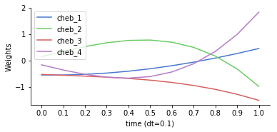
With specifically crafted $t$ or coefficient scaling, we could get more complex and controlled behavior, but that would require careful engineering. More generally, we have guarantees that a matrix computed by a given $\phi$ will be well-conditioned after projecting it onto the orthogonal manifold.

2.5 Orthogonal Projection via Householder Reflections

We adopt the following scheme for orthogonal manifold projection. Given a set of unconstrained parameters $\mathbf{u}_{1},\dots,\mathbf{u}_{d}\in\mathbb{R}^{d}\setminus\{\mathbf{0}\}$ and $s\in\{-1,+1\}$, we map them onto the orthogonal group, $\mathcal{O}(d)$, with the following.

Lemma 1 (Mhammedi et al., 2017).

For $\mathbf{u}_{1},\dots,\mathbf{u}_{d}\in\mathbb{R}^{d}\setminus\{\mathbf{0}\},s\in\{-1,+1\}$ define a function

$$\mathcal{M}(\mathbf{u}_{1},\dots,\mathbf{u}_{d},s)=s\cdot\mathcal{H}(\mathbf{u}_{1})\dots\mathcal{H}(\mathbf{u}_{d}),$$

where

$$\mathcal{H}(\mathbf{u})=\mathbf{I}_{d}-2\frac{\mathbf{u}\mathbf{u}^{\top}}{\|\mathbf{u}\|_{2}^{2}}$$

is a Householder reflection matrix parameterized by $\mathbf{u}$. Then $\mathcal{M}$ is a surjective function into $\mathcal{O}(d)$.

We use $\mathbf{u}_{1},\dots,\mathbf{u}_{d}$ as learnable parameters and take $s=1$ for simplicity. The presented Householder reflection approach has been evaluated in the context of recurrent neural networks (Mhammedi et al., 2017) and normalizing flows (van den Berg et al., 2018).

We test this reparameterization scheme on an 4-degree Poly-NANODE and compare to standard batch-norm in Figure 3, finding that it significantly improves stability.

Figure 3: Here, the learning curves of two NANODEs with 4-degree Chebyshev polynomial basis functions illustrate how poorly selected bases lead to learning collapse. The non-orthogonal variant with batch norm only experiences learning collapse, while learning stability is preserved by orthogonal re-parameterization. This procedure is costly, thus motivating our choice of the trigonometric polynomial or random feature bases.

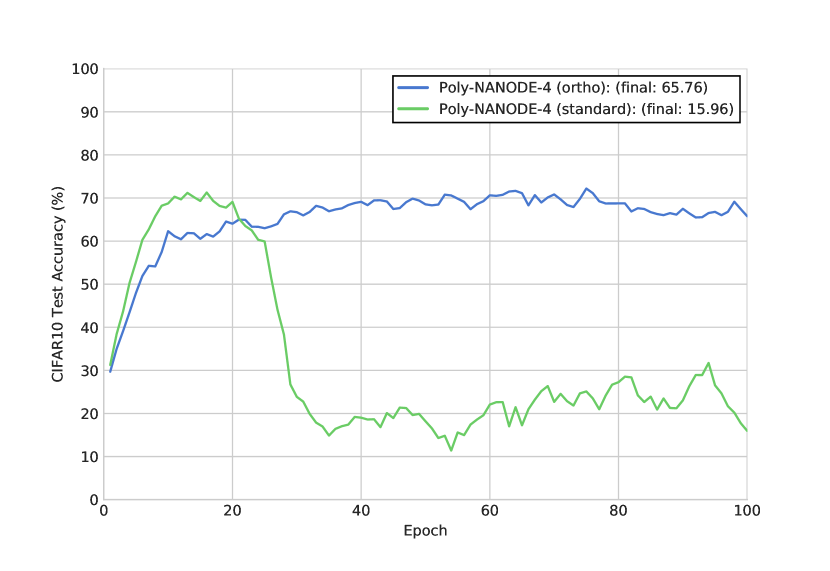
Although multiplying a vector by $\mathcal{H}(\mathbf{u}_{i})$ is of $O(d)$ time complexity, we find that sequential application of $d$ Householder reflections is slower in practice than efficient matrix-vector multiplication product when using unconstrained weights. Therefore, while the orthogonal reparameterization approach of Householder reflections resolves scale and conditioning issues (ensuring stability), trigonometric polynomials (which can be interpreted as a special case of direct optimization along the orthogonal manifold) are preferable.

3 Theoretical Results

3.1 Trigonometric Polynomials and Evolution on Compact Manifolds

Equipped with different methods, for constructing time-varying weights, we will now establish an interesting connection between some of these techniques and flows on compact manifolds.

We need a few definitions. Recall that an orthogonal group is defined as: $\mathcal{O}(N)=\{Q\in\mathbb{R}^{N\times N}:Q^{\top}Q=I_{N}\}$. Manifold $\mathcal{O}(N)$ was already a key actor in the mechanism involving Householder reflections (see: Sec. 2.5). Interestingly, it appears also in the context of proposed parameterizations with trigonometric polynomials, as we show below.

Denote by $\mathcal{T}_{Q}(\mathcal{O}(N))$ linear space tangent to $\mathcal{O}(N)$ in $Q$ (see: Lee (2012)). It can be proven that:

$$\mathcal{T}_{Q}(\mathcal{O}(N))=\{Q\Omega:\Omega\in\mathbb{R}^{N\times N}\text{ and }\Omega^{\top}=-\Omega\}.$$ (13)

Space $\mathcal{T}_{Q}(\mathcal{O}(N))$ can be interpreted as a local linearization of $\mathcal{O}(N)$ in the neighborhood of $Q$.

The geodesics on $\mathcal{O}(N)$ passing through fixed $Q\in\mathcal{O}(N)$ and tangent to $Q\Omega\in\mathcal{T}_{Q}{(\mathcal{O}(N))}$ are of the form: $\gamma_{\Omega}(t)=Q\mathrm{exp}(t\Omega)$. Let $H_{i,j}$ for $1\leq i<j\leq d$ be defined as: $H_{i,j}[i,j]=1$, $H_{i,j}[j,i]=-1$ and $H_{i,j}[k,l]=0$ for other $(k,l)$. Geodesics corresponding to the canonical basis $\{QH_{i,j}:1\leq i<j\leq d\}$ of $\mathcal{T}_{Q}(\mathcal{O}(N))$ have very special form, namely:

$$\gamma_{i,j}(t)=QG^{t}_{i,j},$$ (14)

where $G^{t}_{i,j}\in\mathbb{R}^{N\times N}$ is the so-called Givens rotation - a matrix of the two-dimensional rotation in the subspace spanned by two canonical vectors $\mathbf{e}_{i},\mathbf{e}_{j}$ and with angle $\theta=t$.

Thus Givens rotations can be thought of as encoding curvilinear coordinates corresponding to the canonical basis of tangent spaces $\mathcal{T}_{Q}(\mathcal{O}(N))$ to $\mathcal{O}(N)$.

That observation is a gateway to establishing the tight connection between time-varying weights encoded by trigonometric polynomials in our architectures and walks on compact manifolds. Notice that coordinate-aligned walks on $\mathcal{O}(N)$ can be encoded via products of Givens rotations as:

$$W=QG^{\theta_{1}}_{i_{1},j_{1}}\cdot...\cdot G^{\theta_{k}}_{i_{k},j_{k}},$$ (15)

where $Q\in\mathcal{O}(N)$.

Now notice that $G_{i_{l},j_{l}}^{\theta_{l}}[i,j]=\cos(\theta_{l})$ for $i=j=i_{l}$ or $i=j=j_{l}$, $G_{i_{l},j_{l}}^{\theta_{l}}[i,j]=-G_{i_{l},j_{l}}^{\theta_{l}}[j,i]=\sin(\theta_{l})$ for $(i,j)=(i_{l},j_{l})$ and $G_{i_{l},j_{l}}$ equals the identity matrix on other entries.

Thus we conclude (using standard trigonometric formulae) that if the walk starts at $Q=I_{N}$, and $\theta_{1}=...=\theta_{k}=\theta$ then the $(i,j)$ entry $W[i,j]$ of $W$ is of the form:

$$W[i,j]=\sum_{s=1}^{k}a_{i,j}^{(s)}\cos(s\theta)+\sum_{s=1}^{k}b_{i,j}^{(s)}\sin(s\theta)$$ (16)

for some coefficients: $\{a_{i,j}^{(s)},b_{i,j}^{(s)}\}_{s=1,...,k}$.

Note that if we take $\theta=t$ and $n=k$, then we get the formula for weights that we obtained through trigonometric polynomials. We see that our proposed mechanism leveraging trigonometric polynomials can be utilized to parameterize weight matrices evolving on the orthogonal group, where polynomial degree encodes number of steps of the walk on $\mathcal{O}(d)$ and time corresponds to step sizes along curvilinear axes (geodesics’ lengths). These observations extend to rectangular weight matrices by conducting analogous analysis on the Stiefel Manifold (Lee, 2012).

3.2 Stability of Neural ODEs with Time-Varying Weights

Analysis of gradient stability in the context of neural ODEs with time-varying weights sheds a light on the intriguing connection between stable NANODEs and flows on compact matrix manifolds as we now discuss.

Consider a Neural ODE of the form introduced in Eqn. 1.

Learning this Neural ODE entails optimizing a loss function $L(\cdot)$ summed over a collection of initial conditions,

$$\theta_{*}=\arg\min_{\theta}\sum_{i}L(x^{i}(t,\theta)),$$

where $i$ indexes the training data. At any final time $t$, by the chain rule, the per-example gradient is given by

$$\frac{\partial L}{\partial\theta}=\frac{\partial L(x(t,\theta))}{\partial x}\frac{\partial x(t,\theta)}{\partial\theta}.$$

As a function of time, the spectrum of the Jacobian of $x(t,\theta)$ with respect to $\theta$ dictates how much the gradient is amplified or diminished. Denoting

$$S(t)=\frac{\partial x(t,\theta)}{\partial\theta}\in{\mathbb{R}}^{n\times k},$$

this Jacobian satisfies sensitivity equations (Khalil & Grizzle, 2002) given by the matrix differential equation,

$$\dot{S} = A(t,\theta)S+B(t,\theta),~{}~{}~{}S_{0}=0$$ (17)

$$A(t,\theta) = \frac{\partial f(x,t,\theta)}{\partial x}(x(t,\theta))$$

$$B(t,\theta) = \frac{\partial f(x,t,\theta)}{\partial\theta}(x(t,\theta)).$$

3.2.1 Linear Time Varying Analysis

Let $z=vec(S)$. Then, we can write Eqn. 17 as,

$$\dot{z}=A(t)z+b(t),$$

where $A(t)=I\otimes A(t,\theta)$ and $b(t)=vec(B(t,\theta))$ (with some notation abuse). The solution to such an Linear Time Varying system (LTV) is given by (Kailath, 1980),

$$z(t)=\Phi(t,t_{0})z_{0}+\int_{t_{0}}^{t}\Phi(t,\tau)b(\tau)d\tau,$$

where $\Phi(t,t_{0})$ is the associated state transition matrix (STM, Kailath, 1980). For sensitivity equations, $z_{0}=0$. Hence, we are interested in the spectrum of,

$$S(t)=vec^{-1}\left(\int_{t_{0}}^{t}\Phi(t,\tau)b(\tau)d\tau\right).$$ (18)

As $t\mapsto\infty$, if $S(t)\mapsto 0$ we experience vanishing gradients and if $\|S(t)\|_{2}\mapsto\infty$, exploding gradients.

3.2.2 The State Transition Matrix

The STM, $\Phi(t,\tau)$, is the solution to the matrix differential equation,

$$\dot{M}=A(t)M,~{}~{}~{}M(\tau)=I.$$ (19)

In general, there is no analytical expression for the STM. Under some conditions though, we have some simplifications. Suppose $A(t)$ commutes with $\int_{0}^{t}A(s)ds$. Then we have

$$\phi(t,\tau)=e^{\int_{\tau}^{t}A(s)ds}.$$

This is true when $A(t)$ is diagonal or when $A(t_{1})$ and $A(t_{2})$ commute for all $t_{1},t_{2}$. See (Kailath, 1980) for details.

3.2.3 Time-varying Neural ODEs

With the machinery developed in previous sections, we are finally ready to turn our attention back to NANODEs. Let us consider Neural ODEs of the form,

$$\dot{x}=\sigma(W(t,\theta)x).$$

Then,

$$A(t,\theta) = diag(\sigma^{\prime}(W(t,\theta)x))W(t,\theta)$$ (20)

$$B(t,\theta) = diag(\sigma^{\prime}(W(t,\theta)x))(x^{T}\otimes I)\Gamma,$$ (21)

where $\Gamma=\frac{\partial vec(W(t,\theta))}{\partial\theta}$.

Even though analysis of the spectrum of matrix $S(t)$ from Eq. 18 is a challenging problem, we make several observations. We conjecture that constructing time-dependent weights in such a way that corresponding matrices $A(t)$ belong to spaces tangent in $I_{N}$ to certain compact matrix manifolds (those tangent spaces are also called Lie algebras if the corresponding manifolds are Lie groups (Lee, 2012)) helps $S(t)$ to stabilize.

To see that, note that under these conditions the solution of Eq. 19 evolves on the compact matrix manifold (Lee, 2012), e.g. on the orthogonal group $\mathcal{O}(N)$ if $A(t)$ belongs to the linear space of skew-symmetric matrices (Hairer, 1999). This implies in particular that $\phi(t,\tau)$ from Eq. 18 is bounded. Therefore gradients do not explode if $\int_{t_{0}}^{t}b(\tau)d\tau$ is bounded. We leave further analysis of the connections between time-varying parameterizations and stability to future work.

Figure 4: Increasing the order of the time-varying function defining a NANODEs dynamics enhances its expressiveness. For these NANODEs with discretization of 100 steps ($dt=0.01$), as the degree of the trigonometric basis scales from 1 to 30, the representational capacity of the network increases, as shown by its ability to fit the training set. The threshold line represents the deepest constrained ResNet baseline that we could train on a single GPU.

Figure 5: Mirroring results on the training set, as we scale the order of the Trigonometric Polynomial from 4 to 10, the expressiveness of the network increases as shown by its generalization performance on the test set. T-NANODE outperforms B-NANODE for order $d<$ discretization, suggesting the benefits of smoothness. Horizontal lines illustrate how unconstrained and constrained ResNet baselines, the largest we could train on a single GPU, compare.

4 Experiments

We conduct a suite of experiments to demonstrate the broad applicability of our NANODE approach.

4.1 Image Classification

We first consider the task of image classification using residual flow architectures defined by successive bottleneck residual blocks. As baselines, we trained two ResNet variants: 1) Uncon-ResNet and 2) Con-ResNet (described in Section 2.1). Uncon-ResNet is a standard ResNet architecture where the weight of each ResNet block are not tied to the weights of other ResNet blocks. Con-ResNet is a ResNet architecture where the weights of each ResNet block are constrained to all utilize the same set of parameters, resembling an autonomous Neural ODE, where the weight at each step are fixed (see Figure 1).

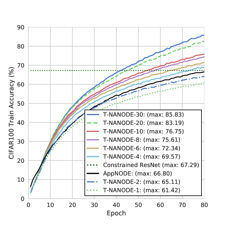
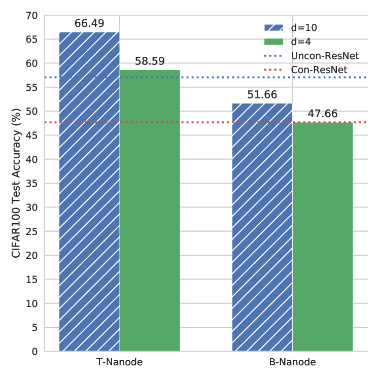
In addition to these baselines, we train several NANODE variants, shown in Figures 5 and 5. Each NANODE has bases $\phi$ of varying orders parameterizing their hidden unit dynamics. Our experiments demonstrate that by making the hidden unit dynamics non-autonomous, we can retain much of the memory benefit of an autonomous ODE (Auto) while achieving performance comparable to that of an Unconstrained ResNet. Furthermore, the memory efficiency benefits granted via the adjoint method allow us to train models significantly ”deeper” than the Unconstrained ResNets and outperform them, as shown in Table 1.

Table 1: Comparison of various architectures for CIFAR-10 and CIFAR-100 image classification tasks. Trigonometric NANODE (T-NANODE-10) outperforms an Autonomous NODE (Auto), as well as the largest Unconstrained ResNet we could train on a single GPU. All the NANODE architectures have a significantly smaller activation memory footprint (ACT. MEM) than the equivalent Unconstrained Resnet. Bucket NANODE (B-NANODE) tended to perform worse than T-NANODE for order $<$ depth. Results averaged across 3 runs, distribution info in supplementary materials.

MODEL	CIFAR10 Acc (%)	CIFAR100 Acc (%)	Act. MEM (GB)	Param Mem (GB)
Auto	82.98	50.33	0.3	2.8e-4
AppNODE	83.20	60.68	0.3	2.8e-4
Con. ResNet	82.35	54.69	3.0	2.8e-4
Uncon. ResNet	86.72	60.91	3.0	2.8e-3
B-NANODE-10	84.38	51.66	0.3	2.8e-3
T-NANODE-10	90.10	66.49	0.3	5.6e-3
B-NANODE-100	93.22	64.06	0.3	2.8e-2

In Figures 5 and 5, we show how we can leverage the order $d$ of $W_{t,ij}=\phi(t,{\alpha})$ to vary the NANODE’s representational capacity. This allows us to elegantly trade off between expressiveness and parameter-efficiency. It is worth noting that parameters typically require far less memory than activations in the CNN or ResNet context. For a reversible architecture such as our NANODEs, with activation memory complexity $\mathcal{O}(1)$, we only need to store our parameters, and the activations of a single Block. However, a standard ResNet with $\mathcal{O}(L)$ activation memory complexity must store activations for all $L$ layers. As shown in Table 1, this means that, for a given memory budget, we can train much wider and deeper neural networks.

In Figure 5, we also compare Bucket and Trigonometric time treatments, the two best performing variants. We find that the trigonometric treatment outperforms the piece-wise, Bucket treatment for order less than the discretization, $d<L$, suggesting the benefits of smoothness. Note, we also experimented with Hypernetwork variants, specified in Eqn. 11 and 12, but obsevered no performance gains over autonomous Neural ODEs, as discussed further in the supplementary materials $A.1$.

4.2 Video Prediction

Leveraging this memory scaling advantage, we consider the problem of video prediction, whereby a model is tasked with generating future frames conditioned upon some initial observation frames. In deterministic settings, e.g. an object sliding with a fixed velocity, a model has to infer the speed and direction from the prior frames to accurately extrapolate. Standard video prediction models can be memory intensive to train. Video tensor activations must contain an additional time dimension that scales linearly as the number of conditioning or generation frames increases. This makes it difficult to simultaneously parameterize powerful models with many filters, and learn long-horizon dynamics.

Figure 6: Loss convergence on a stochastic video prediction task. Here, the total loss of an autonomous NODE, SVG baseline, and a NANODE are compared on the Moving MNIST dataset. The NANODE converges far faster than the SVG baseline and requires a smaller memory footprint. Even after 10 hours of training, the SVG baseline still cannot match the loss reached by the NANODE after the first epoch.

Table 2: Comparison in performance of different architectures on both the MNIST and BAIR Robot Pushing Small (BRP) video prediction datasets. The Evidence Lower Bound (ELBO) and the memory footprint of the network’s activations and parameters are shown. The NANODE model is able to significantly outperform the SVG and NODE models on both tasks, while keeping a small activation memory (ACT. MEM) footprint similar to the Autonomous NODE (Auto) architecture.

MODEL	MNIST (-ELBO)	BRP (-ELBO)	Act. Mem (GB)	Param Mem (GB)
Auto	3.3e-5	9.0e-5	4.7	4.6e-3
SVG	2.2e-5	9.5e-5	4.9	4.6e-3
NANODE	8.5e-6	7.6e-5	4.7	1.9e-2

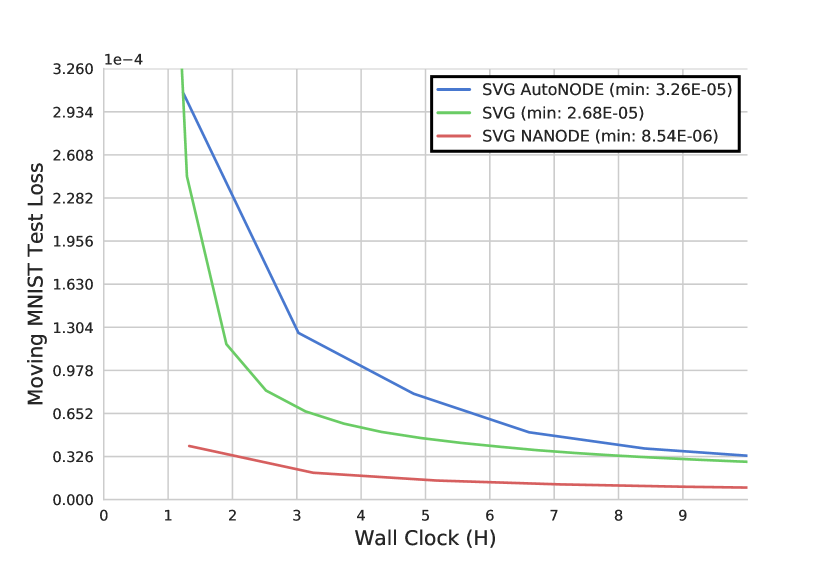
Experiments are conducted using the Moving MNIST (Srivastava et al., 2015) and BAIR Robot Pushing Small (Finn et al., 2016) video datasets. We train an Encoder-Decoder Stochastic Video Generation (SVG) model with a learned prior, based on Denton & Fergus (2018). The baseline architecture contains VGG blocks (Simonyan & Zisserman, 2014) of several dimension preserving CNN blocks with $3\times 3$ filters and $1\times 1$ stride, followed by $2\times 2$ max-pooling operations with stride $2\times 2$. For our NANODE alternative, we replace the 2 out of every 3 CNN layers with a single NANODE block composed of trigonometric polynomial basis $\phi(t,\theta_{ij})$ of discretization $dt=0.33$ and order 3. We train this reversible model on a single GPU, and are able to achieve faster convergence and lower final loss on both tasks compared to the more memory intensive baseline. Figure 6 and Table 2 illustrate the min loss achieved and memory usage of the respective architectures. There is much potential to further improve these video prediction architectures by pairing ideas regarding optimal width vs. depth scaling (Tan & Le, 2019) with the arbitrary depth scaling ability and expressiveness that NANODEs provide.

5 Conclusion

This work explores various constructions of non-autonomous Neural ODEs (NANODE). Treating the weights of these Neural ODE as well-conditioned functions of time enables the weights to vary in complex ways over the course of integration. The class of non-autonomous Neural ODEs presented in this work are strictly more expressive than autonomous ODEs with fixed weights at every time point while enjoying the same small memory footprint. We have also shown that with specific constructions of time dependent weight matrices, performance of non-autonomous ODEs can match unconstrained equivalent ResNets, and even outperform them in memory constrained environments.

Furthermore, we discover an intriguing connection between the stability of NANODEs and flows on compact manifolds. We suggest in future work it would be interesting to further explore designing stable NANODE architectures by leveraging techniques from matrix manifold theory. We also note the potential to apply NANODEs to larger scale video prediction and 3D tasks as a promising direction.

References

- Bengio et al. (1994) Bengio, Y., Simard, P., and Frasconi, P. Learning long-term dependencies with gradient descent is difficult. IEEE transactions on neural networks, 5(2):157–166, 1994.
- Chen et al. (2018) Chen, T. Q., Rubanova, Y., Bettencourt, J., and Duvenaud, D. K. Neural ordinary differential equations. In Advances in neural information processing systems, pp. 6571–6583, 2018.
- Denton & Fergus (2018) Denton, E. and Fergus, R. Stochastic video generation with a learned prior. arXiv preprint arXiv:1802.07687, 2018.
- Dupont et al. (2019) Dupont, E., Doucet, A., and Teh, Y. W. Augmented neural odes. In Advances in Neural Information Processing Systems, pp. 3134–3144, 2019.
- Finn et al. (2016) Finn, C., Goodfellow, I., and Levine, S. Unsupervised learning for physical interaction through video prediction. In Advances in neural information processing systems, pp. 64–72, 2016.
- Glorot & Bengio (2010) Glorot, X. and Bengio, Y. Understanding the difficulty of training deep feedforward neural networks. In Proceedings of the thirteenth international conference on artificial intelligence and statistics, pp. 249–256, 2010.
- Gomez et al. (2017) Gomez, A. N., Ren, M., Urtasun, R., and Grosse, R. B. The reversible residual network: Backpropagation without storing activations. In Advances in neural information processing systems, pp. 2214–2224, 2017.
- Grathwohl et al. (2018) Grathwohl, W., Chen, R. T., Bettencourt, J., Sutskever, I., and Duvenaud, D. Ffjord: Free-form continuous dynamics for scalable reversible generative models. arXiv preprint arXiv:1810.01367, 2018.
- Ha et al. (2016) Ha, D., Dai, A., and Le, Q. V. Hypernetworks. arXiv preprint arXiv:1609.09106, 2016.
- Haber & Ruthotto (2017) Haber, E. and Ruthotto, L. Stable architectures for deep neural networks. Inverse Problems, 34(1):014004, 2017.
- Hairer (1999) Hairer, E. Numerical geometric integration. 1999.
- He et al. (2016) He, K., Zhang, X., Ren, S., and Sun, J. Deep residual learning for image recognition. In Proceedings of the IEEE conference on computer vision and pattern recognition, pp. 770–778, 2016.
- Helfrich et al. (2017) Helfrich, K., Willmott, D., and Ye, Q. Orthogonal recurrent neural networks with scaled cayley transform. arXiv preprint arXiv:1707.09520, 2017.
- Hochreiter (1991) Hochreiter, S. Untersuchungen zu dynamischen neuronalen netzen. Diploma, Technische Universität München, 91(1), 1991.
- Kailath (1980) Kailath, T. Linear systems, volume 156. Prentice-Hall Englewood Cliffs, NJ, 1980.
- Khalil & Grizzle (2002) Khalil, H. K. and Grizzle, J. W. Nonlinear systems, volume 3. Prentice hall Upper Saddle River, NJ, 2002.
- Lee (2012) Lee, J. Introduction to smooth manifolds. 2nd revised ed, volume 218. 01 2012. doi: 10.1007/978-1-4419-9982-5.
- Lezcano-Casado & Martínez-Rubio (2019) Lezcano-Casado, M. and Martínez-Rubio, D. Cheap orthogonal constraints in neural networks: A simple parametrization of the orthogonal and unitary group. arXiv preprint arXiv:1901.08428, 2019.
- Mhammedi et al. (2017) Mhammedi, Z., Hellicar, A., Rahman, A., and Bailey, J. Efficient orthogonal parametrisation of recurrent neural networks using householder reflections. In Proceedings of the 34th International Conference on Machine Learning-Volume 70, pp. 2401–2409. JMLR. org, 2017.
- Miyato et al. (2018) Miyato, T., Kataoka, T., Koyama, M., and Yoshida, Y. Spectral normalization for generative adversarial networks. arXiv preprint arXiv:1802.05957, 2018.
- Nair & Hinton (2010) Nair, V. and Hinton, G. E. Rectified linear units improve restricted boltzmann machines. In Proceedings of the 27th international conference on machine learning (ICML-10), pp. 807–814, 2010.
- Simonyan & Zisserman (2014) Simonyan, K. and Zisserman, A. Very deep convolutional networks for large-scale image recognition. arXiv preprint arXiv:1409.1556, 2014.
- Srivastava et al. (2015) Srivastava, N., Mansimov, E., and Salakhudinov, R. Unsupervised learning of video representations using lstms. In International conference on machine learning, pp. 843–852, 2015.
- Tan & Le (2019) Tan, M. and Le, Q. V. Efficientnet: Rethinking model scaling for convolutional neural networks. arXiv preprint arXiv:1905.11946, 2019.
- van den Berg et al. (2018) van den Berg, R., Hasenclever, L., Tomczak, J. M., and Welling, M. Sylvester normalizing flows for variational inference, 2018.
- Zhang et al. (2019) Zhang, H., Gao, X., Unterman, J., and Arodz, T. Approximation capabilities of neural ordinary differential equations. arXiv preprint arXiv:1907.12998, 2019.