Charmonium properties from lattice QCD + QED: hyperfine splitting, $J/\psi$ leptonic width, charm quark mass and $a_{\mu}^{c}$

Abstract

We have performed the first $n_{f}=2+1+1$ lattice QCD computations of the properties (masses and decay constants) of ground-state charmonium mesons. Our calculation uses the HISQ action to generate quark-line connected two-point correlation functions on MILC gluon field configurations that include $u/d$ quark masses going down to the physical point, tuning the $c$ quark mass from $M_{J/\psi}$ and including the effect of the $c$ quark’s electric charge through quenched QED. We obtain $M_{J/\psi}-M_{\eta_{c}}$ (connected) = 120.3(1.1) MeV and interpret the difference with experiment as the impact on $M_{\eta_{c}}$ of its decay to gluons, missing from the lattice calculation. This allows us to determine $\Delta M_{\eta_{c}}^{\mathrm{annihiln}}$ =+7.3(1.2) MeV, giving its value for the first time. Our result of $f_{J/\psi}=$ 0.4104(17) GeV, gives $\Gamma(J/\psi\rightarrow e^{+}e^{-})$=5.637(49) keV, in agreement with, but now more accurate than experiment. At the same time we have improved the determination of the $c$ quark mass, including the impact of quenched QED to give $\overline{m}_{c}(3\,\mathrm{GeV})$ = 0.9841(51) GeV. We have also used the time-moments of the vector charmonium current-current correlators to improve the lattice QCD result for the $c$ quark HVP contribution to the anomalous magnetic moment of the muon. We obtain $a_{\mu}^{c}=14.638(47)\times 10^{-10}$, which is 2.5$\sigma$ higher than the value derived using moments extracted from some sets of experimental data on $R(e^{+}e^{-}\rightarrow\mathrm{hadrons})$. This value for $a_{\mu}^{c}$ includes our determination of the effect of QED on this quantity, $\delta a_{\mu}^{c}=0.0313(28)\times 10^{-10}$.

I Introduction

The precision of lattice QCD calculations has been steadily improving for some time and is now approaching, or has surpassed, the 1% level for multiple quantities. Good examples are the masses and decay constants of ground-state pseudoscalar mesons Tanabashi et al. (2018). The meson masses can be used to tune, and therefore determine, quark masses. The decay constants can be combined with experimental annihilation rates to leptons to determine elements of the Cabibbo-Kobayashi-Maskawa matrix. The accuracy of modern lattice QCD results means that sources of small systematic uncertainty that could appear at the percent level need to be understood. At this level QED effects, i.e. the fact that quarks carry electric as well as color charge, come into play. A naive argument that such effects could be $\mathcal{O}(\alpha_{\mathrm{QED}})$ would imply a possible 1% contribution. One key driver for the lattice QCD effort to include QED effects has been that of calculations of the hadronic vacuum polarisation (HVP) contribution to the anomalous magnetic moment of the muon, $a_{\mu}$. New results are expected soon from the Muon $g-2$ experiment at Fermilab Grange et al. (2015) which aims to clarify the observed tension between experiment and Standard Model theory seen by the Brookhaven E821 experiment Bennett et al. (2004). Current lattice QCD calculations have reached the precision of a few percent for $a_{\mu}$ and the systematic uncertainties, for example from neglecting QED effects, have become a major focus of attention (see, for example Boyle et al. (2017); Giusti et al. (2019); Borsanyi et al. (2020)).

QED effects can have large finite-volume corrections within a lattice QCD calculation because the Coulomb interaction is long-range. For electrically neutral correlation functions, such as the ones needed for a calculation of the HVP, and that we study here, this is much less of an issue (and we demonstrate this). Since $\alpha^{n}_{s}\alpha_{\mathrm{QED}}$ is not very different in size from $\alpha_{\mathrm{QED}}$ at hadronic scales, calculations must be fully nonperturbative in QCD. A consistent calculation must also allow for the retuning of quark masses needed when QED effects are included.

Here we examine the properties of ground-state charmonium mesons more accurately than has been possible in previous lattice QCD calculations. Since it is possible to obtain statistically very precise results for the charmonium system it is a good place to study small systematic effects from QED and other sources. We are able to see such effects in our results and quantify them. We include $u$, $d$, $s$ and $c$ quarks in the sea for the first time and have results on gluon field configurations with physical $u/d$ sea quarks. We also analyse the impact of including an electric charge on the valence $c$ quarks (only). This approximation, known as ‘quenched QED’, should capture the largest QED effects and enable us to see how much of a difference QED makes. For the vector ($J/\psi$) meson properties we improve on earlier results by using an exact method to renormalise the lattice vector current (both in QCD and QCD+QED). To tune the $c$ quark mass we use the $J/\psi$ meson mass, taking into account the retuning that is required when QED is switched on. We find the impact of this to be of similar size to the more direct QED effects.

The quantities that we focus on here are the masses and decay constants of the ground-state $\eta_{c}$ and $J/\psi$ mesons, the $c$ quark mass and the contribution of the $c$ vacuum polarisation to $a_{\mu}$.

The correlation functions that we calculate in our lattice QCD and QCD+QED calculations are ‘connected’ correlation functions i.e. they are constructed from combining charm quark propagators from the source to the sink. We do not include diagrams in which the $c$ and $\overline{c}$ quarks annihilate to multiple gluons and hence hadrons. We can gain some insight into the effect this annihilation channel has on the meson masses by looking at the meson widths, which are twice the imaginary part of the mass and are dominated by hadronic channels. The $J/\psi$ has a tiny width of 93 keV Tanabashi et al. (2018) but the pseudoscalar $\eta_{c}$ can annihilate to two gluons, allowing it to mix with other flavour-singlet pseudoscalars, and it has a width of 32 MeV Tanabashi et al. (2018). The annihilation channel might then be expected to have a larger impact on the $\eta_{c}$ mass and lead lattice QCD calculations of the mass from connected correlators to disagree with experiment. The only way to achieve the $\mathcal{O}(1\,\mathrm{MeV})$ accuracy required to see this is to determine the mass difference between the $J/\psi$ and $\eta_{c}$ (the hyperfine splitting). Any shift in the $\eta_{c}$ mass will have a much larger (by a factor of 30) relative effect in this splitting. Previous lattice QCD calculations of the hyperfine splitting from connected correlation functions have not been accurate enough to see a significant difference with experiment. Here, for the first time, we can see such a difference because we have very good control both of discretisation effects and sea-quark mass effects and can also determine the impact of QED on this quantity.

A further place in which QED effects need to be quantified, given our accuracy, is that of the determination of the $c$ quark mass. We do this by tuning our results to the experimental $J/\psi$ meson mass with and without electric charge on the valence $c$ quarks and also determine the small change in the mass renormalisation factor, $Z_{m}$, needed to convert to the standard $\overline{\text{MS}}$ mass.

Our analysis of the vector charmonium correlation functions with a completely nonperturbative renormalisation of the vector current allows much improved accuracy in the determination of the leptonic decay width of the $J/\psi$. Using the same correlators, we determine the charm quark portion of the hadronic vacuum polarisation contribution to the anomalous magnetic of the muon, $a_{\mu}^{\text{HVP,c}}$, along with the impact of quenched QED on this quantity. We can compare this to phenomenological results from $R(e^{+}e^{-}\rightarrow\text{hadrons})$.

The paper is laid out as follows:

• Section II describes the lattice QCD calculation and the inclusion of quenched QED;

• Section III describes our determination of the hyperfine splitting;

• Section IV, the $c$ quark mass;

• Section V, the $J/\psi$ and $\eta_{c}$ decay constants;

• Section VI the time-moments of $c$ vector-vector correlators and the $c$ quark hadronic vacuum polarisation contribution to $a_{\mu}$;

• Section VII gives our conclusions.

Each section of results includes a description of the pure QCD calculation followed by a determination of the impact of quenched QED on the result and then a discussion subsection including comparison to both experiment and previous lattice QCD calculations, where applicable. Finally Section VII collects up all of our results and summarises our conclusions.

II Lattice setup

We perform calculations on a total of 17 gluon field ensembles, concentrating our analysis on 15 of these. 16 sets include the effects of light, strange and charm quarks in the sea with up and down quarks having the same mass ($n_{f}=2+1+1$), one set has up and down quarks set separately to their physical values ($n_{f}=1+1+1+1$). All gluon field ensembles include sea quarks using the HISQ action Follana et al. (2007) and were generated by the MILC collaboration Bazavov et al. (2013, 2018a). Parameters for the ensembles are given in Table 1. Our sets include lattices at 6 different $\beta$ (the bare QCD coupling) values corresponding to 6 different sets of lattice spacing values with the finest lattice reaching a spacing of $\sim 0.03$ fm. Although ‘topology freezing’ has been seen on the very finest lattices used here, we do not expect this to have significant impact on the charmonium quantities we study here because no valence light quarks are involved in the calculations Bernard and Toussaint (2018). We use ensembles with sea $u/d=l$ masses at the physical point on all but the finest two lattice spacings. We also employ three ensembles (sets 5, 6 and 7) with shared parameters except for their spatial extent in units of the lattice spacing $L_{s}$. These ensembles allow us to investigate finite volume effects in our QED analysis. We test the impact of strong-isospin breaking effects in the sea by using two ensembles (sets 3A and 3B) with all parameters the same except that one ensemble has $m_{u}=m_{d}=m_{l}$ and one has $(m_{u}+m_{d})/2=m_{l}$ and $m_{d}/m_{u}=2.18$. The gluon action on these ensembles is improved so that discretisation errors through $\mathcal{O}(\alpha_{s}a^{2})$ are removed Hart et al. (2009).

Table 1: Details of the lattice gluon field ensembles and calculation parameters used. The lattice spacing is determined from the Wilson flow parameter, $w_{0}$ Borsanyi et al. (2012), with $w_{0}/a$ values given in column 2. The lattice spacing can be determined in fm by using $w_{0}=0.1715(9)$ fm Dowdall et al. (2013) (fixed from $f_{\pi}$). $L_{s}$ and $L_{t}$ are the lattice spatial and temporal extents in lattice units. Columns 6, 7 and 8 give the sea quark masses in lattice units. Note that all of the configuration sets are $n_{f}=2+1+1$, i.e. with equal mass $u$ and $d$ quarks (denoted $l$) except for set 3B which is $n_{f}=1+1+1+1$. For set 3B $am^{\text{sea}}_{u}$ and $m^{\text{sea}}_{d}$ are listed separately with $am^{\text{sea}}_{u}$ on top. $am_{c}^{\mathrm{val}}$ is the valence $c$ quark mass with $\epsilon_{\mathrm{Naik}}$ the corresponding Naik parameter (see text). The column headed $N_{\mathrm{cfg}}\times N_{t}$ shows both the number of configurations used in the pure QCD calculation and the number of time sources for propagators per configurations. $N_{\mathrm{cfg,QED}}$ refers to the number of configurations (and time sources) used in QCD+QED calculations. Sets 1-3 will be referred to as very coarse ($a\approx$ 0.15 fm), sets 4-8 as coarse ($a\approx$ 0.12fm), sets 9-11 as fine ($a\approx$ 0.09 fm), 12 and 13 as superfine ($a\approx$ 0.06 fm), 14 as ultrafine ($a\approx 0.045$ fm) and 15 as exafine ($a\approx$ 0.03 fm).

Set	$\beta$	$w_{0}/a$	$L_{s}$	$L_{t}$	$am_{l}^{\text{sea}}$	$am_{s}^{\text{sea}}$	$am_{c}^{\text{sea}}$	$am_{c}^{\mathrm{val}}$	$\epsilon_{\mathrm{Naik}}$	$N_{\mathrm{cfg}}\times N_{t}$	$N_{\mathrm{cfg,QED}}\times N_{t}$
1	5.80	1.1119(10)	16	48	0.013	0.065	0.838	0.888	-0.3820	1020$\times$8	-
2	5.80	1.1272(7)	24	48	0.0064	0.064	0.828	0.873	-0.3730	1000$\times$8	340$\times$16
3	5.80	1.1367(5)	32	48	0.00235	0.0647	0.831	0.863	-0.3670	1000$\times$8	-
3A	5.80	1.13215(35)	32	48	0.002426	0.0673	0.8447	0.863	-0.3670	1762$\times$16	-
3B	5.80	1.13259(38)	32	48	0.001524	0.0673	0.8447	0.863	-0.3670	1035$\times$16	-
					0.003328						-
4	6.00	1.3826(11)	24	64	0.0102	0.0509	0.635	0.664	-0.2460	1053$\times$8	-
5	6.00	1.4029(9)	24	64	0.00507	0.0507	0.628	0.650	-0.2378	-	340$\times$16
6	6.00	1.4029(9)	32	64	0.00507	0.0507	0.628	0.650	-0.2378	1000$\times$8	220$\times$16
7	6.00	1.4029(9)	40	64	0.00507	0.0507	0.628	0.650	-0.2378	-	220$\times$16
8	6.00	1.4149(6)	48	64	0.00184	0.0507	0.628	0.643	-0.2336	1000$\times$8	-
9	6.30	1.9006(20)	32	96	0.0074	0.037	0.440	0.450	-0.1250	300$\times$8	-
10	6.30	1.9330(20)	48	96	0.00363	0.0363	0.430	0.439	-0.1197	300$\times$8	371$\times$16
11	6.30	1.9518(7)	64	96	0.00120	0.0363	0.432	0.433	-0.1167	565$\times$8	-
12	6.72	2.8941(48)	48	144	0.00480	0.0240	0.286	0.274	-0.0491	1019$\times$8	265$\times$16
13	6.72	3.0170(23)	96	192	0.0008	0.022	0.260	0.260	-0.0443	100$\times$8	-
14	7.00	3.892(12)	64	192	0.00316	0.0158	0.188	0.194	-0.0250	200$\times$8	-
15	7.28	5.243(16)	96	288	0.00223	0.01115	0.1316	0.138	-0.0127	100$\times$4	-

On these gluon field configurations we calculate propagators for valence $c$ quarks by solving the Dirac equation for a source consisting of a set of Gaussian random numbers across a timeslice (a random wall source). We use multiple time sources per configuration to improve statistical accuracy. The number of configurations used and the number of time sources is given in Table 1. The table also gives the valence $c$ quark masses in lattice units, which may differ from those in the sea because they are tuned more accurately. This will be discussed further below. The HISQ action Follana et al. (2007) includes an improved discretisation of the covariant derivative in the Dirac equation. This removes tree-level $a^{2}$ discretisation errors by the addition of a 3-link ‘Naik’ term to the symmetric 1-link difference. For heavy quarks the coefficient of the Naik term is adjusted from 1 to $1+\epsilon_{\mathrm{Naik}}$ to remove $(am)^{4}$ errors at tree-level Follana et al. (2007). A closed-form expression for $\epsilon$ in terms of the tree-level quark pole mass is given in Monahan et al. (2013) along with the formula for the tree-level quark pole mass in terms of the bare mass. Table 1 gives the values of $\epsilon$ that we use.

We combine charm quark and antiquark propagators to calculate two types of quark-line connected two-point correlation functions: pseudoscalar and vector. The ground state of the pseudoscalar correlation function corresponds to the $\eta_{c}$ meson and the vector correlation function, to the $J/\psi$. When using staggered quarks, as here, the different spin structures are implemented using position dependent phases in the operators at source and sink. The two-point ‘Goldstone’ pseudoscalar ($\gamma_{5}\otimes\gamma_{5}$ in spin-taste notation) correlation functions are simply constructed from quark propagators $S(x,0)$ from the origin to $x$ as

$$C(t)=\frac{1}{4}\sum_{x}\langle\mathrm{Tr}(S(x,0)S^{\dagger}(x,0))\rangle,$$ (1)

where the factor of 4 accounts for the taste multiplicity with staggered quarks. For the vector correlation functions we use a local vector operator (spin-taste $\gamma_{i}\otimes\gamma_{i}$). The correlation functions then combine $S(x,0)$ with a propagator made from patterning the source with a phase $(-1)^{x_{i}}$ and inserting $(-1)^{x_{i}}$ at the sink timeslice as we tie the propagators together and sum over spatial sites. Our vector correlation functions average over all spatial polarisations, $i$, for improved statistical precision. Note that we do not calculate any quark-line disconnected correlation functions.

The HISQ local vector current is not conserved and requires renormalisation. For this purpose we use the RI-SMOM momentum subtraction scheme implemented on the lattice as discussed in Hatton et al. (2019). In Hatton et al. (2019) it was shown that, because of the Ward-Takahashi identity, these renormalisation factors do not suffer any contamination by nonperturbative artefacts (condensates) and can therefore be safely used in calculations such as those presented here. The quenched QED correction to the RI-SMOM vector current renormalisation was also given in Hatton et al. (2019) and shown to be tiny ($\sim 0.01\%$) for the HISQ action (as expected since the pure QCD $Z_{V}$ values only differ from 1 at the 1% level and quenched QED provides a small correction to this difference from 1). Here we use the $Z_{V}$ values from Hatton et al. (2019) at a scale $\mu$ of 2 GeV. We will also demonstrate (see Section V) that using $\mu$ = 3 GeV gives the same result as it must for a $Z_{V}$ that correctly matches the lattice to continuum physics.

Since we make use of an ensemble (set 14) with a finer lattice spacing than those studied in Hatton et al. (2019) we have directly calculated the value of $Z_{V}$ on set 14 at $\mu=2$ GeV in addition. We have, however, only used a small number of configurations (6) in that calculation due to the computational limitation of the stringent Landau gauge fixing required. We therefore double the statistical uncertainty for $Z_{V}$ on that ensemble. This has very little impact on our final results as the $Z_{V}$ uncertainty is small. See Appendix A for a discussion of our $Z_{V}$ values, where we also derive a $Z_{V}$ value for set 15.

In order to tune the mass of the valence charm quark we use bare charm mass values on each lattice that produce a $J/\psi$ mass equal to the experimental value (both in pure QCD and in QCD+QED). We choose the $J/\psi$ here rather than the $\eta_{c}$ because the relatively large width of the $\eta_{c}$ means that annihilation effects that we are not including could lead to small (order 0.1% ) uncertainties in the mass. This is mentioned in Section I and will be discussed further in Section III. We measure our valence $c$ mass mistunings as the difference between our lattice $J/\psi$ mass and the experimental average value of 3.0969 GeV (with negligible uncertainty) Tanabashi et al. (2018). The two panels of Fig. 2, where the horizontal line is the experimental value, show that our mistunings are well below 0.5%. These mistunings are allowed for in our final fits.

II.1 Two-point correlator fits

We fit the two-point correlation functions described above as a function of the time separation, $t$, between source and sink. The aim is to extract the energies (masses) and amplitudes (giving decay constants) of the ground-state mesons in each channel. However it is important to allow for the systematic effect of excited states that are present in the correlation functions and can affect the ground-state values if they are not taken into account. We do this by fitting the correlators to sums of exponentials associated with each energy eigenvalue and using Bayesian priors to constrain the (ordered) excited states in the standard way Lepage et al. (2002). The pseudoscalar correlators are fit to

$$C_{P}(t) = \sum_{i}A^{P}_{i}f(E^{P}_{i},t),$$ (2)

$$f(E,t) = e^{-Et}+e^{-E(T-L_{t})}\,.$$

The vector correlators require a more complicated form because of the presence of opposite parity states as a result of the use of staggered quarks:

$$C_{V}(t)=\sum_{i}\left(A^{V}_{i}f(E^{V}_{i},t)-(-1)^{t}A^{V,o}_{i}f(E^{V,o}_{i},t)\right).$$ (3)

We cut out the correlator values at low values of $t$, below some value $t_{\mathrm{min}}$ ($5-10$) where excited state contamination is most pronounced. We also use a standard procedure (see Appendix D of Dowdall et al. (2019)) to avoid underestimating the low eigenvalues of the correlation matrix and hence the uncertainty.

The fit parameters that we need from Eq. 2 and 3 are the mass of the ground-state ($E^{P}_{0}$ and $E^{V}_{0}$) and the amplitude ($A^{P}_{0}$ and $A^{V}_{0}$). From the amplitude we determine the decay constant, see Section V.

II.2 QED formalism

We perform calculations in both lattice QCD and in lattice QCD with quenched QED. By quenched QED we mean that we include effects from the valence quarks having electric charge but we neglect effects from the electric charge of the sea quarks. We will first describe how we include QED and then discuss the expected impact on our results of not including the QED effects from the sea quarks.

To include quenched QED effects we generate a random momentum space photon field $A_{\mu}(k)$ in Feynman gauge for each QCD gluon field configuration. This choice of gauge simplifies the generation of the photon field as the QED path integral weight takes the form of a Gaussian with variance $1/\hat{k}^{2}$ where $\hat{k}=2\mathrm{sin}(k_{\mu}/2)$. The results presented here do not depend on this gauge choice. Once the momentum space field is generated zero modes are set to zero using the QED_L formulation Hayakawa and Uno (2008). $A_{\mu}$ is then Fourier transformed into position space. We have checked that these Feynman gauge $A_{\mu}$ fields produce the plaquette and average link expected from $\mathcal{O}(\alpha_{\mathrm{QED}})$ perturbation theory (readily obtained from $\mathrm{O}(\alpha_{s})$ calculations in lattice QCD with Wilson glue Weisz (1983); Hart et al. (2004)). These gauge fields are exponentiated as $\mathrm{exp}(ieQA_{\mu})$ to give a U(1) field which is then multiplied into the QCD gauge links before HISQ smearing. $Q$ is the quark electric charge in units of the proton charge $e$.

This approach is known as the stochastic approach to quenched QED Duncan et al. (1996), in contrast to the perturbative approach of de Divitiis et al. (2013). Since $\mathcal{O}(\alpha_{\mathrm{QED}})$ is already a very small effect, we are seeking here only to pin down the linear term in $\alpha_{\mathrm{QED}}$, fully nonperturbatively in $\alpha_{s}$. The two approaches should then give the same result to our level of accuracy; we use the stochastic approach because it is more straightforward (in the quenched case) and gives very precise results for the $c$ quarks we are interested in here.

II.3 Impact of quenching QED

Quenched QED affects only the valence quarks; the sea quarks remain uncharged. We expect the valence quark contribution to be by far the largest QED effect (although already very small as we will see) and discuss here the small systematic error that remains from ignoring sea quark QED effects. The impact of having $m_{u}=m_{d}$ in the sea for most of our results is at the same level and we also discuss that.

We first discuss the determination of the lattice spacing in QCD with quenched QED. In such a calculation there is no coupling of QED effects to purely gluonic quantities. This means that the Wilson flow parameter $w_{0}/a$, measured on each ensemble, is unchanged from pure QCD. The physical value of $w_{0}$ that is used to determine the lattice spacing on each ensemble was determined in Dowdall et al. (2013) by matching the decay constant of the $\pi$ meson, $f_{\pi}$, in lattice QCD to that obtained from experiment. The experimental value of $f_{\pi}$ is obtained from measurement of the rate for $\pi\rightarrow\ell\nu[\gamma]$ decay where $[\gamma]$ indicates that the rate is fully inclusive of additional photons. The rate obtained is then adjusted to remove electromagnetic and electroweak corrections and to give a ‘purely leptonic rate’ corresponding to weak annihilation at lowest order in the absence of QED Rosner et al. (2018). Combining this with a determination of $|V_{ud}|$ from nuclear $\beta$ decay Tanabashi et al. (2018) gives an experimental value of $f_{\pi}\equiv f_{\pi}^{\mathrm{expt}}$ which is a ‘pure QCD’ value, albeit that for a physical $\pi^{+}$ meson. The dominant uncertainty in $f_{\pi}^{\mathrm{expt}}$ is that from the remaining uncertainty in the electromagnetic corrections to the experimental rate, mainly from the hadronic-structure dependent contributions to the emission of additional photons. This is set at 0.1% in Rosner et al. (2018).

Because $f_{\pi}^{\mathrm{expt}}$ is a pure QCD quantity it can be used to set the lattice spacing in lattice QCD in a way that should be minimally different for lattice QCD+QED. Small differences might still be expected between the lattice QCD $f_{\pi}$ and the experimental value from the way that the quark masses are tuned in a pure QCD scenario. The lattice QCD calculation in Dowdall et al. (2013) used $m_{u}=m_{d}$ and tuned the average mass, $m_{l}$, to the experimental mass of the $\pi^{0}$, which is the mass that both neutral and charged $\pi$ mesons have in the absence of QED, up to quadratic corrections in the $u-d$ mass difference. An uncertainty was included in the $\pi^{0}$ mass to allow for these corrections, taking an estimate from chiral perturbation theory Amoros et al. (2001). We expect the impact of such effects to be tiny, well below 0.1%. They are at the same level as potential effects from QED in the sea and would therefore be only possible to pin down with a calculation that included the impact of having electrically charged quarks in the sea.

These expectations are backed up by recent lattice QCD+QED results Borsanyi et al. (2020) that used the $\Omega$ baryon mass to determine $w_{0}$. The impact of QED for the sea quarks was included to first order in $\alpha_{\mathrm{QED}}$. No effects linear in $m_{u}-m_{d}$ are expected in $M_{\Omega}$ because, like $f_{\pi}$ and $M_{\pi}$ above, it is symmetric under $u\leftrightarrow d$ interchange. Strong-isospin breaking effects were therefore ignored. The impact of QED in the sea on $w_{0}M_{\Omega}$ was found to be $\mathcal{O}(0.01\%)$, whereas the effect of QED for the valence quarks (already allowed for in the $f_{\pi}$ analysis) was $\mathcal{O}(0.05\%)$. The final value of $w_{0}$ using $M_{\Omega}$ from Borsanyi et al. (2020) agrees well with the result using $f_{\pi}$ from Dowdall et al. (2013), although the uncertainties in both cases are completely dominated by those from the pure QCD, isospin-symmetric part of the calculation.

From this we conclude that, at the sub-0.1% level, we can compare lattice QCD plus quenched QED with pure lattice QCD using the same value of the lattice spacing, determined from $f_{\pi}$, in both calculations.

The impact of quenching QED on charmonium quantities follows a similar discussion to that for the lattice spacing because interaction with the electric charge of the sea quarks is suppressed by sea quark mass effects and by powers of $\alpha_{s}$. Since the sum of electric charges of $u$, $d$ and $s$ sea quarks is zero, QED interaction between valence $c$ quarks and light sea quarks will be suppressed by sea quark mass differences. The impact of $c$ quarks in the sea is already small and so we can safely neglect the even smaller QED effects from valence/sea $c$ quark interactions. The leading sea-quark QED effect will then come from photon exchange across a sea-quark bubble at $\mathcal{O}(\alpha_{s}^{2}\alpha_{\mathrm{QED}})$ Hatton et al. (2019) in perturbative language. The expected size is then 10% of that of the QED effects from valence $c$ quark interactions, which we will see are themselves typically a small fraction of 1%..

II.4 Impact of having $m_{u}=m_{d}$ in the sea

As discussed above, we expect the effects of having $m_{u}=m_{d}$ in the sea, i.e. not including strong-isospin breaking effects, to be negligible. For both the scale-setting determination and for the charmonium quantities themselves, pure strong-isospin breaking effects are quadratic in $(m_{u}-m_{d})/\Lambda$. Effects linear in the sea quark masses are already small, for example an $\mathcal{O}(5\,\mathrm{MeV})$ shift in the average $u/d$ quark mass produces a 1% effect on $w_{0}/a$ Chakraborty et al. (2015). We might then expect quadratic effects to be $\mathcal{O}(0.01\%)$.

We can provide a test of these expectations from results on gluon ensemble sets 3A and 3B that differ only in the values of $m_{u}$ and $m_{d}$ in the sea for the same average (which has its physical value). Set 3B has $m_{d}/m_{u}$ set to the expected ratio Basak et al. (2019). We see from Table 1 that the determinations of $w_{0}/a$ agree at the level of their 0.03% uncertainties. In contrast, the $w_{0}/a$ value on set 3A differs by a clearly visible 0.40(5)% from that on set 3, which has sea quark masses that are slightly mistuned from the physical point by an amount (summing over $u$, $d$ and $s$) equal to 5% Chakraborty et al. (2015) of $m_{s}$.

Table 2 compares values for the $J/\psi$ and $\eta_{c}$ masses in lattice units on these two ensembles for the same $am_{c}^{\mathrm{val}}$ and the ratio of the two results is plotted in Figure 1. The meson masses in lattice units agree on the two ensembles to within their statistical errors which are at the level of 0.001%. We also tabulate results for the decay constants and plot the ratio of these values. Again agreement is seen between results on set 3A and set 3B. They provide a weaker constraint because of much larger statistical errors, but nevertheless they agree within 0.05%. Notice that this comparison does not allow for possible changes in $w_{0}/a$ in the two cases. As discussed above, this could be at the 0.01% level. Again we can contrast the agreement between sets 3A and 3B with the results on set 3 where, for the same $am_{c}^{\text{val}}$, the $\eta_{c}$ mass differs by 0.02%.

We conclude that we can safely neglect strong-isospin breaking in the sea and proceed with calculations on gluon field ensembles with $m_{u}^{\mathrm{sea}}=m_{d}^{\mathrm{sea}}$.

Table 2: Results for the $\eta_{c}$ and $J/\psi$ masses and decay constants (see Section V for how these are calculated) in lattice units on gluon field ensembles sets 3A and 3B (Table 1). Both sets have the average $u/d$ quark mass in the sea set to its physical value but set 3B has $m_{d}/m_{u}$ also set to the expected ratio. The valence $c$ quark mass was set to 0.863 in lattice units.

	3A ($n_{f}$=2+1+1)	3B ($n_{f}$=1+1+1+1)
$aM_{\eta_{c}}$	2.288139(19)	2.288131(25)
$aM_{J/\psi}$	2.375618(44)	2.375585(60)
$af_{\eta_{c}}$	0.366596(38)	0.366588(41)
$af_{J/\psi}/Z_{V}$	0.41799(16)	0.41790(24)

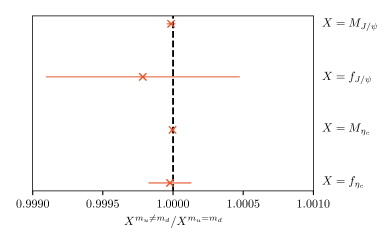
Figure 1: A test of the impact of strong-isospin breaking in the sea through a comparison of results for the charmonium quantities given in Table 2 for sets 3A and 3B (Table 1). These sets differ only in the $u/d$ quark masses in the sea. Set 3A has $m_{u}=m_{d}$ and set 3B has $m_{d}/m_{u}=2.18$ with the same average value. The plot above gives the ratio of results in lattice units, for the same $am_{c}^{\mathrm{val}}$, for the $J/\psi$ and $\eta_{c}$ masses and decay constants. The masses agree to within their 0.001% statistical errors and the decay constants agree to within their statistical errors (0.05% for the $J/\psi$).

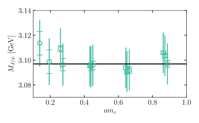
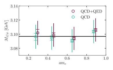
Figure 2: Top panel: Pure QCD $J/\psi$ masses on all 15 sets from Table 1 using the valence masses in that Table. Two error bars are shown. The error can be broken into parts that are uncorrelated between different sets and the contribution from fixing the lattice spacing from the physical value of $w_{0}$ which is correlated. The outer error bar shows the full uncertainty and the inner bar the uncertainty without the contribution from $w_{0}$. Bottom panel: The $J/\psi$ masses on sets 2, 6, 10 and 12 with and without the inclusion of quenched QED. On each set the same valence mass (and lattice spacing) was used for both pure QCD and QCD+QED but the points have been separated on the $x$-axis for clarity. The error bars are the same as for the top panel, but note that here there is a correlation of the uncertainty from $w_{0}/a$ for the QCD and QCD+QED results on each set. The QCD+QED results are above the pure QCD results in every case.

II.5 A first look at quenched QED effects

An estimate of the size of corrections from quenched QED (often simply referred to as QED in what follows) in charmonium systems can be obtained by studying the effect on the $J/\psi$ mass. The bottom panel of Fig. 2 shows the $J/\psi$ mass for the same valence $c$ mass for both QCD+QED and pure QCD calculations on sets 2, 6, 10 and 12. The QCD+QED and QCD results at the same lattice spacing are separated on the $x$-axis for clarity. All points share a correlated uncertainty (the outer error bar) from $w_{0}$ and this dominates the uncertainty. The uncorrelated error is shown by the smaller inner error bar. Note that the points at the same lattice spacing are also correlated through their $w_{0}/a$ value. The shift of the mass in QCD+QED compared to pure QCD is very small, at the level of 0.1%, and is upwards.

When discussing QCD+QED and pure QCD calculations of some quantity $X$ we will use the notation $X[\mathrm{QCD}+\mathrm{QED}]$ and $X[\mathrm{QCD}]$ respectively. We will often consider the ratio of the two for which we will use the shortened notation $R^{(0)}_{\mathrm{QED}}[X]$. $R^{0}_{\mathrm{QED}}$ will refer to the ‘bare’ ratio defined using the same bare quark mass $am_{c}$ in both QCD+QED and pure QCD calculations. $R_{\mathrm{QED}}$ will refer to the final QED-renormalised ratio which includes the impact of retuning the $c$ quark mass to give the experimental $J/\psi$ mass in both the QCD+QED and pure QCD cases. So

$$R^{0}_{\mathrm{QED}}[X] \equiv \left.\frac{X[\mathrm{QCD+QED}]}{X[\mathrm{QCD}]}\right|_{{\mathrm{fixed}}\,am_{c}}$$ (4)

$$R_{\mathrm{QED}}[X] \equiv \left.\frac{X[\mathrm{QCD+QED}]}{X[\mathrm{QCD}]}\right|_{{\mathrm{fixed}}\,M_{J/\psi}}\,.$$

As shown in Fig. 2 the bare $c$ quark mass has to be re-adjusted downwards for QCD+QED relative to pure QCD.

II.6 Fitting strategy

We have results in pure QCD for all of the sets in Table 1 and QCD+QED results on a subset of ensembles. To be able to simultaneously account both for the ‘direct’ effects of QED and for the effects of valence $c$ mass mistuning, which may be similarly sized, we choose to fit all of this data in a single fit for each quantity we consider. The generic form of the fit we use for a quantity $X$ is

$$X(a^{2},Q) = x\bigg{[}1+\sum_{i=1}^{5}c_{a}^{(i)}(am_{c})^{2i}+$$

$$c_{m,{\mathrm{sea}}}\delta_{m}^{\mathrm{sea},uds}\{1+c_{a^{2},\mathrm{sea}}(\Lambda a)^{2}+c_{a^{4},\mathrm{sea}}(\Lambda a)^{4}\}+$$

$$c_{c,{\mathrm{sea}}}\delta_{m}^{\mathrm{sea},c}+c_{c,\mathrm{val}}\delta_{m}^{\mathrm{val},c}+$$

$$\alpha_{\mathrm{QED}}Q^{2}\{c_{\mathrm{QED}}+\sum_{p=1}^{3}c_{aQ}^{(p)}(am_{c})^{2p}+c_{\mathrm{val},Q}\delta_{m}^{\mathrm{val},c}\}\bigg{]}.$$

Here $Q$ is the valence quark electric charge (in units of $e$) used in the calculation and is therefore 0 in pure QCD. The pure QCD value of this fit at the physical point (the continuum limit with quark masses set to their physical values) is $x$. The value including quenched QED corrections is $x[1+\alpha_{\mathrm{QED}}Q^{2}c_{\mathrm{QED}}]$. Note that the factor of $\alpha_{\mathrm{QED}}$ multiplying the QED part of the fit function is there so that the fit parameters are order 1. The stochastic method that we use includes in principle all orders of $\alpha_{\mathrm{QED}}$ but we expect to see only linear terms, including $\alpha_{\mathrm{QED}}\alpha_{s}^{n}$ pieces.

Our fits are typically to 15 pure QCD data points and 4 QCD+QED points. The pure QCD points do not include those on sets 6 and 7 which are used to test finite-volume effects or on sets 3A and 3B that are used to test strong-isospin breaking effects, but they do include additional results at mistuned $c$ quark masses to test mistuning effects.

We now describe each of the terms in Eq. (II.6) in turn. The $(am_{c})^{i}$ terms on the first line account for discretisation effects. Because we are dealing with heavy quarks here, the scale of discretisation effects can be set by $m_{c}$ and will typically be larger than those for light-quark quantities. Since $m_{c}>\Lambda_{\mathrm{QCD}}$ any discretisation effects set by scale $\Lambda_{\mathrm{QCD}}$ will simply appear as $m_{c}$-scale discretisation effects with a small coefficient.

The terms on the second line allow for mistuning of the sea $u/d$ and $s$ masses and discretisation effects in that mistuning (we shall see that those are important for the hyperfine splitting). The total of the mistuning of the sea masses is defined as in Chakraborty et al. (2015):

$$\delta_{m}^{\mathrm{sea},uds}=\frac{2m_{l}^{\mathrm{sea}}+m_{s}^{\mathrm{sea}}-2m_{l}^{\mathrm{phys}}-m_{s}^{\mathrm{phys}}}{10m_{s}^{\mathrm{phys}}}.$$ (6)

$m_{s}^{\mathrm{phys}}$ is taken from Chakraborty et al. (2015) or, where not available on the finest lattices, calculated from the tuned $c$ quark mass and the $m_{c}/m_{s}$ ratio given in Chakraborty et al. (2015). The value of $\Lambda$ in the discretisation effects multiplying the sea-quark mistuning is taken as 1 GeV ($\sim m_{c}$).

The effect of mistuning the charm mass in the sea is included in the third line of Eq. (II.6) using

$$\delta_{m}^{\mathrm{sea},c}=\frac{m_{c}^{\mathrm{sea}}-m_{c}^{\mathrm{phys}}}{m_{c}^{\mathrm{phys}}}.$$ (7)

The values of $m_{c}^{\mathrm{phys}}$ are taken from Chakraborty et al. (2015). Although this used a slightly different tuning method the differences are negligible for this purpose. We have tested that including discretisation effects for this term has no effect on the fit.

Mistuning in the valence mass is accounted for through $\delta_{m}^{\mathrm{val},c}$ on the third and fourth lines of Eq. (II.6). We define this as

$$\delta_{m}^{\mathrm{val},c}=\frac{M_{J/\psi}-M^{\mathrm{expt}}_{J/\psi}}{M^{\mathrm{expt}}_{J/\psi}}.$$ (8)

where $M_{J/\psi}$ is our lattice result for that ensemble in either the QCD or the QCD+QED case. Thus $\delta_{m}^{\mathrm{val},c}$ is zero (the valence $c$ quark mass is tuned) when the $J/\psi$ mass takes its experimental value on each ensemble (and with or without QED). The fit parameters $c_{c,\mathrm{val}}$ and $c_{\mathrm{val},Q}$ then determine the dependence on the valence $c$ mass of the quantity being fit, and the QED corrections to that dependence, respectively. The experimental value of the $J/\psi$ mass is 3.0969 GeV Tanabashi et al. (2018) with negligible uncertainty.

In order to make use of the correlations between our QCD+QED and pure QCD results on the same gluon field configurations we perform simultaneous fits to the correlators in each case. The fits then capture the correlations and we can propagate them to the fit of Eq. (II.6). At the same time it allows us to determine the ratio of QCD+QED to pure QCD for the quantities that we will study. We will give results for these ratios in the sections that follow.

The fit form of Eq. (II.6) has been constructed such that the coefficients (apart from $x$) are expected to be of order 1. We therefore use priors of $0\pm 1$ for all fit parameters except $x$ for which we take a prior width on its expected value of 20% (the prior mean for $x$ depends on the quantity being fitted).

III Hyperfine splitting

III.1 Pure QCD

Table 3: The $\eta_{c}$ and $J/\psi$ masses and their difference ($a\Delta M_{\mathrm{hyp}}$) in pure QCD on each set in lattice units. The values of $am_{c}^{\mathrm{val}}$ are those given in Table 1 except for two cases with a deliberately mistuned $c$ quark mass: set 6 denoted by a * where $am_{c}=0.643$ and set 14 denoted by a ${\dagger}$ where $am_{c}$=0.188. The pseudoscalar and vector correlator fits have been performed separately and the correlations between $aM_{\eta_{c}}$ and $aM_{J/\psi}$ have therefore been ignored because they have little impact.

Set	$aM_{\eta_{c}}$	$aM_{J/\psi}$	$a\Delta M_{\mathrm{hyp}}$
1	2.331899(72)	2.42072(19)	0.08883(20)
2	2.305364(39)	2.39308(14)	0.08772(14)
3	2.287707(26)	2.37476(21)	0.08705(21)
4	1.876536(48)	1.94364(10)	0.06710(11)
6	1.848041(35)	1.914749(67)	0.066708(76)
6∗	1.834454(34)	1.901479(66)	0.067025(74)
8	1.833950(18)	1.900441(39)	0.066491(43)
9	1.366839(72)	1.41568(16)	0.04884(17)
10	1.342455(21)	1.391390(43)	0.048935(48)
11	1.329313(18)	1.378237(51)	0.048924(54)
12	0.896675(24)	0.929860(54)	0.033185(59)
13	0.862689(22)	0.895650(37)	0.032961(43)
14	0.666818(39)	0.691981(54)	0.025163(67)
14†	0.652439(56)	0.67798(14)	0.02554(15)
15	0.496991(47)	0.516126(68)	0.019135(82)

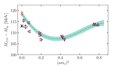
Figure 3: The charmonium hyperfine splitting as a function of lattice spacing on pure QCD ensembles. Our results are from ensembles including $u$, $d$, $s$ and $c$ quarks in the sea with varying $u/d$ average quark mass. The raw lattice results, for well-tuned $c$ quark masses, are given by symbols with error bars. The error bars include both statistical uncertainties and those from determining the lattice spacing from $w_{0}$, which are correlated between values. The results on each group of ensembles with approximately the same lattice spacing are given the same symbol. Within these groups, the results go from right to left as the $u/d$ quark mass changes from $m_{s}/5$ to the physical value. Notice the small range on the $y$-axis; this is the results of discretisation effects being so small for the HISQ action. Results at mistuned $c$ masses are not plotted but are included in the fit. The fit line is the output of the fit from Eq. (II.6) at physical quark masses and with $Q=0$. The orange cross gives our result in the continuum limit for physical quark masses. The black cross gives the experimental average result Tanabashi et al. (2018).

Table 4: QCD+QED $\eta_{c}$ and $J/\psi$ masses and hyperfine splitting presented as the ratio of the QCD+QED result to the pure QCD one on that set. Correlations between the calculations in the QCD+QED and pure QCD cases are used in the determination of the ratio and result in the very high statistical accuracy obtained. Note that the ratio is calculated for the same $am_{c}$ value in the two cases i.e. the ratio given here does not include the impact of retuning the $c$ quark mass.

Set	$R^{0}_{\mathrm{QED}}[M_{\eta_{c}}]$	$R^{0}_{\mathrm{QED}}[M_{J/\psi}]$	$R^{0}_{\mathrm{QED}}[\Delta M_{\mathrm{hyp}}]$
2	1.000450(26)	1.000750(27)	1.0086(10)
6	1.0008335(59)	1.0010742(81)	1.00774(28)
10	1.0011861(54)	1.0014044(76)	1.00739(26)
12	1.0015755(48)	1.001787(11)	1.00750(33)

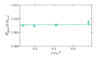
Figure 4: The fractional effect of quenched QED on the charmonium hyperfine splitting plotted against $(am_{c})^{2}$. The fractional effect is determined at the same $am_{c}$ value, i.e. it does not include $c$ quark mass retuning effects. The dashed line is horizontal and shows the weighted average value. The results show the precision that can be obtained by capitalising on the correlations between QCD+QED and QCD. This enables a clear demonstration that the impact of quenched QED here is not dependent on the lattice spacing.

The hyperfine splitting, $\Delta M_{\mathrm{hyp}}$, is calculated on each ensemble as the difference of the vector and pseudoscalar ground state masses, in lattice units, divided by the lattice spacing. The results for $aM_{\eta_{c}}$ and $aM_{J/\psi}$ and their difference are given in Table 3 for the pure QCD case. Although the pseudoscalar and vector correlators on each configuration are correlated the fit outputs for the vector correlator dominate the uncertainties and so the correlations have very little effect as a result.

The pure QCD results are plotted in Fig. 3 along with the fit form of Eq. (II.6) for the pure QCD case (i.e. $Q=0$). Note the small range of the $y$-axis - this is possible for our results because we have a highly-improved quark action with small discretisation errors. Since all tree-level $a^{2}$ errors have been removed, the shape of the curve reflects the fact that higher-order $a^{4}$ and $a^{6}$ errors are visible; discretisation errors of this kind are present in all formalisms of course, but often they are hidden below much larger $a^{2}$ effects and consequently overlooked. Note also the clear dependence on the light sea quark mass seen on the finest lattices. To pin down the value of the valence mass mistuning parameter, $c_{\mathrm{val}}$, we include results at deliberately mistuned $c$ quark masses (see Table 3). These are not shown in the Figure but are included in the fit. The result for the hyperfine splitting in the pure QCD case in the continuum limit and for physical quark masses is 118.6(1.1) MeV, which is higher than the experimental average value, as is clear in Fig. 3. In order to understand what this means, we need to quantify all possible sources of small systematic effects in our calculation, including those from QED.

III.2 Impact of Quenched QED

The fractional direct effect of quenched QED on the $\eta_{c}$ and $J/\psi$ masses and the hyperfine splitting are given in Table 4. The correlation between the QCD+QED and the pure QCD results enables very high statistical accuracy to be obtained in the ratio. The inclusion of quenched QED shifts both the $\eta_{c}$ and $J/\psi$ masses up by $\mathcal{O}(0.1\%)$, depending on lattice spacing, at a given $am_{c}$ value. Although these mass shifts are small, there is a difference between the shift for the $J/\psi$ and that for $\eta_{c}$ and so the inclusion of quenched QED also changes the hyperfine splitting. The impact here is more substantial,  0.7%, because the hyperfine splitting is so much smaller. The size of the direct QED effect on the hyperfine splitting can be simply estimated by replacing $C_{F}\alpha_{s}$ by $Q^{2}\alpha_{\mathrm{QED}}$ in a potential model estimate of the splitting. This gives a fractional effect of $\alpha_{\mathrm{QED}}/(3\alpha_{s})$, consistent with what we find.

The values of $R^{0}_{\mathrm{QED}}[\Delta M_{\mathrm{hyp}}]$ are plotted against $(am_{c})^{2}$ in Fig. 4. This shows that the results are consistent across all lattice spacings and thus discretisation effects in this ratio are smaller than for the masses themselves.

Finite-volume effects are an issue in general for QED corrections to meson masses but we expect them to be small for the electrically neutral and spatially small charmonium mesons that we study here. In Davoudi and Savage (2014) it is shown that the finite volume expansion for electrically neutral mesons starts at $\mathcal{O}(1/L_{s}^{4})$. In Fig. 5 we compare results for the fractional effect of QED on the $J/\psi$ and $\eta_{c}$ as a function of $1/L_{s}$. This calculation is done on sets 5, 6 and 7 (see Table 1) which differ only in their spatial extent. We see no finite-volume effects to well within 0.01%, and we therefore ignore such effects.

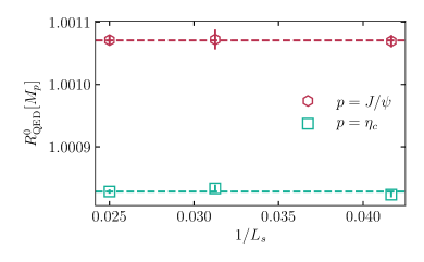
Figure 5: The fractional shift in the $J/\psi$ and $\eta_{c}$ masses from the inclusion of quenched QED plotted as a function of $1/L_{s}$ on sets 5, 6 and 7. The dashed lines are horizontal lines at the weighted average values.

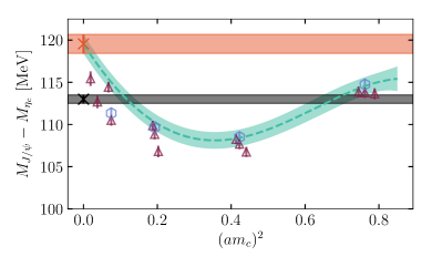
Figure 6: The charmonium hyperfine splitting as a function of lattice spacing, including both QCD+QED and pure QCD points. The red open triangles are the same lattice results as in Fig. 3. The additional QCD+QED points are given as blue open hexagons. The green fit band is the output of the fit from Eq. (II.6), but now with the $c$ quark electric charge, $Q=2/3$. The orange cross and orange band gives our result in the continuum limit for physical quark masses. The black cross and black band gives the experimental average result Tanabashi et al. (2018).

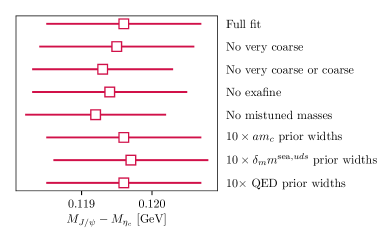
Figure 7: A stability analysis for our fit (see text) to the charmonium hyperfine splitting. Our full fit result is shown at the top. The lines with error bars below this show the result for different modifications of this fit. From the top, these include missing out results on particular sets of configurations, then missing out the results using mistuned $c$ quark masses and then changing the priors by a factor of ten on different sets of parameters in the fit.

Our results including both pure QCD and QCD+QED are shown in Fig. 6, plotted against $(am_{c})^{2}$. The fit curve from Eq. (II.6) at physical quark masses is also shown. The fit has a $\chi^{2}/\mathrm{dof}$ of 0.59 and gives a hyperfine splitting in the continuum limit at physical quark masses of 119.6(1.1) MeV. In Figure 7 we show the results of a stability analysis for this fit. The figure shows that the fit is very robust.

Taking the (correlated) ratio between the physical value of the full QCD+QED fit and the physical value from the fit at $Q=0$ (i.e. the pure QCD result) we obtain $R_{\mathrm{QED}}[\Delta M_{\mathrm{hyp}}]=$ 1.00804(43). This ratio now does include the effect of retuning the $c$ quark mass to obtain the experimental $J/\psi$ mass when quenched QED is included. This retuning requires a reduction of the bare $c$ quark mass by $\mathcal{O}(0.1\%)$ (see Table 4) and this further increases the hyperfine splitting, but only by $\mathcal{O}(0.1\%)$. The impact of QED here is therefore dominated by the ‘direct’ quenched QED effect.

There is an additional pure QED contribution to the $J/\psi$ mass that has not been included yet since it is quark-line disconnected. This comes from a diagram in which the $c\overline{c}$ annihilate into a photon which converts back into $c\overline{c}$. The contribution of this diagram is

$$\frac{8\pi\alpha_{\mathrm{QED}}Q^{2}}{M_{J/\psi}^{2}}|\psi(0)|^{2},$$ (9)

where $\psi(0)$ is the nonrelativistic $J/\psi$ wavefunction equal (in the normalisation being used here) to $f_{J/\psi}\sqrt{M_{J/\psi}}/\sqrt{6}$ Gray et al. (2005). The contribution evaluates to +0.7 MeV, which is a tiny, and completely negligible, effect for the $J/\psi$ meson mass (0.03%). It has some impact on the hyperfine splitting because that is 30 times smaller and so we include it here. We add this contribution to our hyperfine splitting result with a 30% uncertainty from possible QCD corrections to give a final result of

$$M_{J/\psi}-M_{\eta_{c}}(\mathrm{connected})=120.3(1.1)\ \mathrm{MeV}.$$ (10)

Table 5: Error budget for our final result for the charmonium hyperfine splitting including quenched QED corrections. The uncertainties shown are given as a percentage of the final result. The largest uncertainties are clearly from the determination of the lattice spacing.

	$\Delta M_{\mathrm{hyp}}$
$a^{2}\to 0$	0.13
Pure QCD statistics	0.24
QCD+QED statistics	0.08
$w_{0}/a$	0.24
$w_{0}$	0.87
Valence mistuning	0.02
Sea mistuning	0.06
Total	0.96

The error budget for our hyperfine splitting result is given in Table 5. We follow Appendix A of Bouchard et al. (2014) for the meaning of the uncertainties contributing to the error budget. The majority of the uncertainty is associated with the lattice spacing determination, either from the correlated $w_{0}$ uncertainty or the individual $w_{0}/a$ uncertainties. This is not surprising because the hyperfine splitting is sensitive to uncertainties in the determination of the lattice spacing for the reasons discussed in Donald et al. (2012). We have separated out the uncertainty arising from the pure QCD data and the $R^{0}_{\mathrm{QED}}[\Delta M_{\mathrm{hyp}}]$ values from Table 4 which we label ‘Pure QCD Statistics’ and ‘QCD+QED Statistics’ in Table 5. The sea mistuning uncertainty comes from the $c_{m}$ coefficients in Eq. II.6 and the valence mistuning uncertainty from the $c_{\mathrm{val}}$ and $c_{\mathrm{val},Q}$ coefficients. The $a^{2}\to 0$ uncertainty is from the $c_{a}$ and $c_{aQ}$ coefficients.

Our final result is for the charmonium hyperfine splitting determined from quark-line connected correlation functions in QCD and including the impact of QED effects, through explicit calculation in quenched QED. We expect the effect of further QED effects in the sea to be negligible compared to our 1% uncertainty. The only significant Standard Model effect then missing is that of quark-line disconnected diagrams in which the $c\overline{c}$ annihilate to gluons. We expect this effect to be much larger for the $\eta_{c}$ than for the $J/\psi$ so a comparison of our result for the hyperfine splitting to experiment can yield information on the size and sign of the annihilation contribution to the $\eta_{c}$ mass. This is discussed in the next subsection.

III.3 Discussion: Hyperfine Splitting

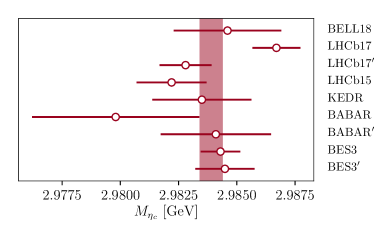
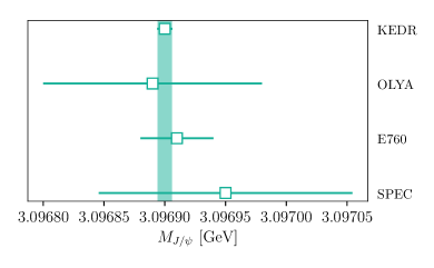
Figure 8: Comparison of different experimental results for the $J/\psi$ and $\eta_{c}$ masses along with the PDG average values. The $\eta_{c}$ results represent a recent subset of those used in the PDG average. The most recent result is from BELLE (denoted BELL18) Xu et al. (2018). There are three different determinations from LHCb Aaij et al. (2015, 2017a, 2017b), two of which also measured the hyperfine splitting. We include a KEDR measurement Anashin et al. (2014), two from different BaBar analyses Lees et al. (2014) and two from BESIII Ablikim et al. (2012a, b).

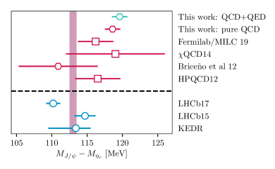
Figure 9: Comparison of different lattice results for the charmonium hyperfine splitting and separate experimental results that measure this difference, as well as the PDG average (pink band). The PDG average is obtained from taking the differences of the PDG $J/\psi$ and $\eta_{c}$ masses (see Fig. 8) rather than only from experiments that directly measure the splitting. The squares give lattice QCD results from calculations that include $n_{f}=2+1$ flavours of quarks in the sea. The hexagons give results that include $n_{f}=2+1+1$ flavours of sea quarks, including the results we present here at the top of the plot. All lattice QCD results have had uncertainties from neglecting $\eta_{c}$ annihilation removed so that we might expect some difference between them and experiment (see text), but previous lattice QCD results have not been accurate enough to see this. The Fermilab/MILC result used Fermilab $c$ quarks on gluon field configurations with asqtad sea quarks DeTar et al. (2019) and the previous HPQCD result Donald et al. (2012) used HISQ quarks on the same asqtad-sea ensembles. Briceño et al Briceno et al. (2012) used a modification of the Fermilab approach known as relativistic heavy quarks on the $n_{f}=2+1+1$ HISQ sea quark ensembles that we use here. The $\chi$QCD result Yang et al. (2015) used overlap quarks on gluon field configurations including $n_{f}=2+1$ domain-wall sea quarks.

The experimental average value of the hyperfine splitting (113.0(5) MeV) from the Particle Data Group (PDG) Tanabashi et al. (2018) is calculated as the difference of the separate averages for the $J/\psi$ and $\eta_{c}$ masses. The different experimental results contributing to the PDG average of the two masses are shown in Fig. 8. For the $J/\psi$ mass the average is dominated by the most recent result from KEDR Anashin et al. (2015). There are only three experimental results used in these analyses that can independently produce values for the hyperfine splitting. These are the KEDR experiment Anashin et al. (2015, 2014) and two LHCb analyses in different channels Aaij et al. (2015, 2017a). The LHCb result in Aaij et al. (2017a) used the $\eta_{c}(2\mathrm{S})\to p\overline{p}$ decay while the analysis of Aaij et al. (2015) used $\eta_{c}(1\mathrm{S})\to p\overline{p}$. In the comparison plot of Fig. 9 Aaij et al. (2015) is referred to as LHCb15 and Aaij et al. (2017a) as LHCb17.

Fig. 9 shows a comparison of lattice QCD results for the charmonium hyperfine splitting along with the PDG average value and separate experimental values that measured this splitting. Previous calculations on gluon field configurations that included $n_{f}=2+1$ flavours of sea quarks by HPQCD Donald et al. (2012) and by Fermilab/MILC DeTar et al. (2019) both obtained values above the experimental average, although only by just over one standard deviation.

The result we present here is substantially more precise than these earlier studies and for the first time displays a significant, 6$\sigma$, difference from the experimental average, clearly showing that the lattice result lies above the experimental one. We interpret this as the effect of ignoring annihilation to gluons in the calculation of the $\eta_{c}$ mass. From the comparison of our results to experiment we conclude that these annihilation effects increase the $\eta_{c}$ mass by 7.3(1.2) MeV, where the uncertainty is dominated by that from the lattice calculation.

Previous analyses of this issue have given mixed results. In NRQCD perturbation theory Follana et al. (2007) we can relate the shift in the $\eta_{c}$ mass to its total (hadronic) width through the perturbative amplitude for $c\overline{c}\rightarrow gg\rightarrow c\overline{c}$ at threshold Bodwin et al. (1995). Then

$$\Delta M_{\eta_{c}} = \frac{\Gamma_{\eta_{c}}}{2}\left(\frac{2(\ln 2-1)}{\pi}+\mathcal{O}(\alpha_{s},v^{2}/c^{2})\right)$$

$$= \frac{31.9(7)}{2}\,\mathrm{MeV}\times\left(-0.195+\mathcal{O}(\alpha_{s},v^{2}/c^{2})\right).$$

The leading term here gives $-$3.1 MeV, but sub-leading corrections could easily change the sign. An alternative way to think about the effect is non-perturbatively and then the gluon annihilation allows mixing between the $\eta_{c}$ and other flavour-singlet pseudoscalar mesons. Since these are lighter than the $\eta_{c}$ this mixing could give a positive correction to the $\eta_{c}$ mass. Direct lattice QCD determination of the effect, by calculating the appropriate quark-line disconnected correlation functions, has so far not proved possible. This is because the lighter states that are introduced by the mixing make it very hard to pin down a small effect on the mass of a particle, the $\eta_{c}$, which is so much further up the spectrum in this channel. An estimate of the mass shift of +1–4 MeV was obtained in the quenched approximation in which this mixing is not possible but where mixing with glueballs could happen instead Levkova and DeTar (2011).

Our result for the hyperfine splitting, by its accuracy, provides for the first time a clear indication of the size of the impact of the $\eta_{c}$ annihilation to gluons on its mass:

$$\Delta M^{\mathrm{annihln}}_{\eta_{c}}=+7.3(1.2)\,\mathrm{MeV}.$$ (12)

IV Determination of $m_{c}$

IV.1 Pure QCD

In Lytle et al. (2018) we showed that it is possible to determine the strange and charm quark masses accurately in lattice QCD using an intermediate momentum-subtraction scheme. By intermediate we mean that the mass renormalisation factor to convert the tuned bare lattice quark mass to the momentum-subtraction scheme is calculated on the lattice. The conversion from the momentum-subtraction to the final preferred $\overline{\text{MS}}$ scheme is carried out using QCD perturbation theory in the continuum. To do this accurately it is important to use a momentum-subtraction scheme that has only one momentum scale, $\mu$. This means that the squared 4-momentum on each leg of the vertex diagram, from which the mass renormalisation factor is calculated, is $\mu^{2}$. The RI-SMOM scheme Sturm et al. (2009) used in Lytle et al. (2018) is such a scheme. A further important point is that the mass renormalisation factor will be contaminated by nonperturbative (condensate) artefacts through its nonperturbative calculation on the lattice. To identify and remove these artefacts (that appear as inverse powers of $\mu$) requires calculations at multiple values of $\mu$ and a fit to the results, as discussed in Lytle et al. (2018).

Below we briefly summarise the procedure followed in Lytle et al. (2018):

1. Determine the tuned bare quark mass and lattice spacing at physical sea quark masses for each set of gluon field configurations at a fixed $\beta$ value. We do this following Appendix A of Chakraborty et al. (2015).

2. Calculate the mass renormalisation factor, $Z_{m}^{\mathrm{SMOM}}$, that converts the lattice quark masses to the RI-SMOM scheme for each $\beta$ value at multiple values of $\mu$. We thereby obtain the quark mass in the RI-SMOM scheme at scale $\mu$.

3. Convert the mass to the $\overline{\mathrm{MS}}$ scheme at scale $\mu$ using a perturbative continuum matching calculation. We denote this conversion factor by $Z_{m}^{\overline{\mathrm{MS}}/\mathrm{SMOM}}(\mu)$.

4. Run all the $\overline{\text{MS}}$ quark masses at a range of scales $\mu$ to a reference scale of 3 GeV using the four loop QCD $\overline{\text{MS}}$ $\beta$ function. We denote these running factors $r(3\ \mathrm{GeV},\mu)$.

5. Fit all of the results for the $\overline{\text{MS}}$ mass at 3 GeV to a function that allows for discretisation effects and condensate contamination, which begins at $1/\mu^{2}$ with the nongaugeinvariant $\langle A^{2}\rangle$ condensate.

6. Obtain from the fit the physical value for the quark mass in the $\overline{\text{MS}}$ scheme at 3 GeV with condensate contamination removed.

Table 6: Lattice spacing values and tuned $c$ quark masses at physical sea quark masses for each group of ensembles at a fixed $\beta$ value, denoted by their name in column 1 (see Table 1). The lattice spacing value is given in units of $w_{0}$ in column 2 and the $c$ quark mass, fixed from the $J/\psi$ meson mass, is given in GeV units in column 3. The first uncertainty on the mass is uncorrelated between lattice spacing values, and the second is correlated.

	$w_{0}/a$	$m_{c}^{\mathrm{tuned}}$ [GeV]
coarse	1.4055(33)	1.0524(10)(30)
fine	1.9484(33)	0.9736(10)(30)
superfine	3.0130(56)	0.8973(10)(30)
ultrafine	3.972(19)	0.8592(20)(30)

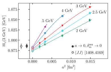
Figure 10: $\overline{m}_{c}(3\ \mathrm{GeV})$ extrapolated to the continuum with a fit form that allows for condensate terms that behave like inverse powers of the renormalisation scale $\mu$. This plot is an updated version of the upper section of Fig. 10 in Lytle et al. (2018), with added data points on ultrafine lattices (set 14) and a retuned bare $c$ quark mass fixed from the $J/\psi$, rather than $\eta_{c}$, meson. The ultrafine points have slightly mistuned $\mu$ values compared to the corresponding lines (see text).

Here we provide three small updates to Lytle et al. (2018). We first list them and then discuss them in more detail below. The three updates are:

1. we improve the uncertainty in the tuning of the bare lattice $c$ quark mass by using the $J/\psi$ mass rather than the $\eta_{c}$;

2. we include results from a finer ensemble of lattices (set 14) to provide even better control of the continuum limit;

3. we use the new 3-loop-accurate SMOM to $\overline{\mathrm{MS}}$ matching factors, $Z_{m}^{\overline{\mathrm{MS}}/\mathrm{SMOM}}$, calculated in Kniehl and Veretin (2020); Bednyakov and Pikelner (2020) to reduce the perturbative matching uncertainty.

The first update is to change how the tuning of the bare charm quark mass is done. In Lytle et al. (2018) bare charm masses were used that had been tuned to the experimental $\eta_{c}$ mass, adjusted to allow for estimates of missing QED (from a Coulomb potential) and gluon annihilation effects (from perturbation theory). A 100% uncertainty was included on the adjustment Chakraborty et al. (2015). Now that we are explicitly including quenched QED it makes more sense to have a tuning process that uses an experimental meson mass with no adjustments. We also want to use the same tuning process for both the pure QCD case and the QCD+QED case to allow for a clear comparison and one that reflects the procedures that would be followed in a complete QCD+QED calculation. This means that we should use the $J/\psi$ meson mass, as we have done in Section III. The $J/\psi$ mass is more accurate experimentally than that of the $\eta_{c}$ and the $J/\psi$ has a much smaller width, implying little effect on the mass from its 3-gluon annihilation mode. The impact of $J/\psi$ annihilation to a single photon is a sub-1 MeV shift to the mass which is a 0.02% effect, so negligible.

Using our $J/\psi$ meson masses and following the procedure of Chakraborty et al. (2015) we obtain tuned bare $c$ masses for each $\beta$ value. These are given in Table 6 along with the $w_{0}/a$ values corresponding to physical sea quark masses at that $\beta$ value, which are also updated slightly from Lytle et al. (2018). These slight changes in $w_{0}/a$ lead to small adjustments in the $\mu$ values relative to those given in Table IV of Lytle et al. (2018). This is accounted for when we run the $Z_{m}$ to the correct reference scale in $\overline{\mathrm{MS}}$.

The second update is to include results from the ultrafine $\beta=7.0$ ensemble (set 14). The appropriate tuned mass and $w_{0}/a$ value for physical sea quark masses is given in Table 6. We have also calculated new $Z_{m}^{\mathrm{SMOM}}(\mu)$ values on set 14. These are given in Appendix A.

The third update is to add the $\alpha_{s}^{3}$ correction to the SMOM to $\overline{\mathrm{MS}}$ conversion factor, $Z_{m}^{\overline{\mathrm{MS}}/\mathrm{SMOM}}$, for the mass renormalisation. This correction was recently calculated in continuum perturbative QCD Kniehl and Veretin (2020); Bednyakov and Pikelner (2020). For $n_{f}=4$, as here, the $\alpha_{s}^{3}$ correction is a small effect (0.2%), continuing the picture seen at $\mathcal{O}(\alpha_{s})$ and $\mathcal{O}(\alpha_{s}^{2})$ and consistent with the uncertainty taken from missing it in Lytle et al. (2018).

Once we have determined results for $\overline{m}_{c}$(3 GeV) at a variety of lattice spacing values using the SMOM intermediate scheme at a variety of $\mu$ values, we need to fit the results to determine $\overline{m}_{c}$(3 GeV) in the continuum limit. We do this following our previous calculation Lytle et al. (2018), where the fit function is given in Eq. (26). The fit includes discretisation effects and condensate artefacts in the lattice calculation of $Z_{m}^{\mathrm{SMOM}}$. In Lytle et al. (2018) we included a term in the fit, $c_{\alpha}\alpha_{s}^{3}(\mu)$ (with $\alpha_{s}$ in the $\overline{\mathrm{MS}}$ scheme) to allow for the then-missing $\alpha_{s}^{3}$ term in the SMOM to $\overline{\mathrm{MS}}$ conversion. Here we replace that term with $c_{\alpha}\alpha_{s}^{4}(\mu)$ since the conversion is now calculated through $\alpha_{s}^{3}$ and included in our results. We take a prior value on $c_{\alpha}$ of $0.0\pm 0.5$. This allows for the coefficient of the $\alpha_{s}^{4}$ term in the conversion factor to be 4 times as large as the $\alpha_{s}^{3}$ coefficient.

Table 7: Error budget (in %) for the calculation of the charm quark mass in the $\overline{\mathrm{MS}}$ scheme at a scale of 3 GeV using RI-SMOM as an intermediate scheme. The listed contributions have the same meaning as those in Lytle et al. (2018) except that we use $r$ here for the running factor rather than $R$ and we have an additional one labelled ‘QED effects’ which comes from the continuum extrapolation shown in Fig. 12.

	$\overline{m}_{c}$(3 GeV)
$a^{2}\to 0$	0.23
Missing $\alpha_{s}^{4}$ term	0.10
Condensate	0.21
$m_{\mathrm{sea}}$ effects	0.00
$Z_{m}^{\overline{\mathrm{MS}}/\mathrm{SMOM}}$ and $r$	0.07
$Z_{m}^{\mathrm{SMOM}}$	0.12
Uncorrelated $m^{\mathrm{tuned}}$	0.15
Correlated $m^{\mathrm{tuned}}$	0.30
Gauge fixing	0.09
$\mu$ error from $w_{0}$	0.12
QED effects	0.02
Total	0.52

The updated fit to our results for $\overline{m}_{c}$ in the $\overline{\text{MS}}$ scheme at 3 GeV is shown in Fig. 10. The fit has a $\chi^{2}/\mathrm{dof}$ of 0.71. The error budget for this calculation is shown in Table 7. Most of the entries are very similar to those in Lytle et al. (2018). The contribution due to the continuum extrapolation has, unsurprisingly, dropped a little, as has the uncertainty from the missing higher order terms (here $\alpha_{s}^{4}$) in the SMOM to $\overline{\mathrm{MS}}$ conversion. The correlated tuning uncertainty comes largely from the uncertainty in the physical value of $w_{0}$ used to fix the lattice spacing. We will be able to reduce that uncertainty in future by improving the determination of the value of $w_{0}$.

Our updated pure QCD result is

$$\overline{m}_{c}(3\,\mathrm{GeV})_{\mathrm{QCD}}=0.9858(51)\,\mathrm{GeV}.$$ (13)

Running this down to a scale equal to the mass gives

$$\overline{m}_{c}(\overline{m}_{c})_{\mathrm{QCD}}=1.2723(78)\,\mathrm{GeV}.$$ (14)

These results improve on and supersede the value in Lytle et al. (2018).

IV.2 Impact of Quenched QED

To include quenched QED effects in the determination of the $c$ quark mass we must determine both the bare quark mass and the mass renormalisation factor with quenched QED switched on.

We include quenched QED effects for $Z_{m}$ in the RI-SMOM scheme in the same way as that described for the vector current renormalisation in Hatton et al. (2019). This involves the generation of U(1) fields in Landau gauge to remain consistent with the Landau gauge QCD configurations used in the pure QCD calculation. When converting from the RI-SMOM scheme for $Z_{m}$ to the $\overline{\mathrm{MS}}$ scheme it is also necessary to include QED effects in the perturbative matching factor. We can evaluate the QED contribution to $Z_{m}^{\overline{\text{MS}}/\text{SMOM}}$ at order $\alpha_{\mathrm{QED}}$ by multiplying the known coefficient of $\alpha_{s}$ Sturm et al. (2009) by (3/4)$Q^{2}$ to give the coefficient of $\alpha_{\mathrm{QED}}$. The impact is very small ($<0.1\%$) and we therefore safely neglect higher order terms. The numerical values of the $\mathcal{O}(\alpha_{\mathrm{QED}})$ term we do include for the RI-SMOM to $\overline{\mathrm{MS}}$ matching are given in Table 8.

Table 8: Table giving factors needed for the determination of the quark mass in a calculation including quenched QED for different $\mu$ values and lattice spacings (denoted by set numbers). The fractional QED correction to $Z_{m}^{\mathrm{SMOM}}$ is given in the third column, the QED component of the RI-SMOM to $\overline{\mathrm{MS}}$ matching for each $\mu$ in the fourth column and the factor giving the QED mass running from $\mu$ to a reference scale of 3 GeV in the fifth column.

Set	$\mu$ [GeV]	$R_{\mathrm{QED}}[Z_{m}^{\text{SMOM}}]$	$Z_{m,\mathrm{QED}}^{\overline{\mathrm{MS}}/\mathrm{SMOM}}$	$r^{\mathrm{QED}}$(3 GeV, $\mu$)
5	2	1.001200(83)	0.999872	0.999372
10	2	1.001516(35)	0.999872	0.999372
12	2	1.001853(83)	0.999872	0.999372
5	2.5	1.000827(31)	0.999873	0.999718
5	3	1.000540(15)	0.999873	-
10	3	1.000851(11)	0.999873	-
12	3	1.001308(18)	0.999873	-
10	4	1.0005001(21)	0.999873	1.000446
12	4	1.0009331(34)	0.999873	1.000446

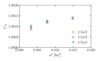
Figure 11: The factor $C_{m}$ that forms part of the QED effect in the lattice to $\overline{\text{MS}}$ mass renormalisation, as defined in Eq. (15), plotted against the square of the lattice spacing. The fact that $C_{m}$, as shown here, has almost no $\mu$ or $a$ dependence demonstrates that the $\mu a$ dependence seen in $R_{\mathrm{QED}}[Z^{\overline{\text{MS}}}_{m}]$ from columns 3 and 4 of Table 8 is simply that expected from perturbation theory.

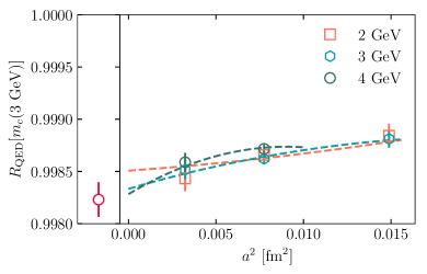
Figure 12: QED correction to the charm quark mass in the $\overline{\mathrm{MS}}$ scheme at a scale of 3 GeV. The different $\mu$ values, shown as different colours and shapes, have all been run to 3 GeV and only differ by discretisation and condensate effects. The red point on the left is the result for $R_{\mathrm{QED}}[\overline{m}_{c}(3\,\mathrm{GeV})]$ returned by the fit of Eq. (IV.2).

To assess the QED impact on the tuned bare $c$ mass we use the QCD+QED $J/\psi$ masses given in Table 4 and shown in Fig. 2. As we have corrected the pure QCD determination of $m_{c}$ to be tuned to the experimental $J/\psi$ mass this is the tuning we will use for the QCD+QED case as well. The fractional shift in $am_{c}$ required to obtain the correct $J/\psi$ mass after QED has been included (which we denote $R_{\mathrm{QED}}[am_{c}]$) can be evaluated from the fractional change in the $J/\psi$ mass. $R_{\mathrm{QED}}[am_{c}]$ is the fractional change in $am_{c}$ required to return the $J/\psi$ mass to the value it had in pure QCD (i.e. the experimental value) once QED is switched on. Thus the increase in $J/\psi$ mass seen with QED must be compensated by a corresponding reduction in $am_{c}$. From the deliberately mistuned $am_{c}$ values in Table 3 we see that the fractional change in the $c$ mass is 1.5 times larger than the change seen in the meson mass. We can use this factor, along with $R^{0}_{\text{QED}}[M_{J/\psi}]$ values from Table 4 and the required change of sign in the shift, to determine the retuning of the quark masses in QCD+QED. We therefore take $R_{\mathrm{QED}}[am_{c}]$ on coarse, fine and superfine lattices (sets 6, 10 and 12) to be 0.99840(8), 0.99790(4) and 0.99734(9) respectively. We increase the uncertainty on $R_{\mathrm{QED}}[am_{c}]$ compared to that for $R^{0}_{\mathrm{QED}}[M_{J/\psi}]$ by a factor of 5 to allow for the uncertainty in our conversion factor of 1.5 above.

We calculate the ratio of $Z_{m}$ in the SMOM scheme in QCD+QED to pure QCD ($R_{\mathrm{QED}}[Z_{m}^{\text{SMOM}}]$) following the methods of Lytle et al. (2018). The calculations are carried out at multiple values of the renormalisation scale $\mu$ and extrapolated to zero valence quark mass. Results are given in Table 8. Notice that these values are larger than 1 and so compensate to a large extent for the changes in the tuning of the bare lattice $am_{c}$ induced by QED. This reflects the fact that most of the shift is an unphysical ultraviolet self-energy effect. We then convert from the SMOM scheme to $\overline{\mathrm{MS}}$ by making use of the ratio of the perturbative conversion factor for QCD+QED to pure QCD, i.e. the $\mathcal{O}(\alpha_{\text{QED}})$ piece of $Z_{m}^{\overline{\text{MS}}/\text{SMOM}}$ also given in Table 8. This is less than 1 but only by a very small amount.

Multiplying these two factors together gives the ratio of the lattice to $\overline{\mathrm{MS}}$ mass renormalisation factors for QCD+QED to that for pure QCD, i.e. $R_{\mathrm{QED}}[Z_{m}^{\overline{\text{MS}}}]$. From Table 8, multiplying columns 3 and 4, we can see that $R_{\mathrm{QED}}[Z_{m}^{\overline{\text{MS}}}]$ varies with $\mu$ and with lattice spacing over a range of about 0.001. In perturbation theory we expect $R_{\mathrm{QED}}[Z_{m}^{\overline{\text{MS}}}]$ to consist of a power series in $\alpha_{\text{QED}}$ and $\alpha_{s}$ multiplied by constants and powers of logarithms of $a\mu$. The leading logarithm at each order can be derived from the anomalous dimensions of the mass, allowing us to write Bednyakov et al. (2017)

$$R_{\mathrm{QED}}[Z_{m}^{\overline{\text{MS}}}]=1+C_{m}-\frac{3\alpha_{\mathrm{QED}}Q^{2}}{4\pi}\log(\mu^{2}a^{2}).$$ (15)

Here $C_{m}$ is a constant, up to discretisation effects and higher order terms multiplying powers of $\log(a\mu)$. Figure 11 plots our results for $C_{m}$. These show very little variation with $a$ and $\mu$, confirming that the dependence on $a$ and $\mu$ of $R_{\mathrm{QED}}[Z_{m}^{\overline{\text{MS}}}]$ is almost entirely captured by Eq. (15).

Once the impact of QED on the $c$ mass in the $\overline{\text{MS}}$ scheme at scale $\mu$ is obtained, as above, we then need to allow for QED effects in the running of the masses from $\mu$ to the reference scale of 3 GeV. This is done by multiplication by a factor $r^{\text{QED}}$ calculated in $\mathcal{O}(\alpha_{\text{QED}})$ perturbation theory and given in Table 8. These numbers are also very close to 1. The $\alpha_{s}\alpha_{\text{QED}}$ term could in principle have some impact here but it is very small and we neglect it Bednyakov et al. (2017).

Multiplying $R_{\text{QED}}[am_{c}]$ and $R_{\text{QED}}[Z_{m}^{\overline{\text{MS}}}]$ together allows us to determine the ratio of the $c$ quark mass in the $\overline{\text{MS}}$ scheme at 3 GeV from QCD+QED to that in pure QCD, i.e. $R_{\mathrm{QED}}[\overline{m}_{c}(3\,\mathrm{GeV})]$. The values that we have for this ratio come from results at multiple values of $\mu$ and multiple values of the lattice spacing. To determine the physical ratio in the continuum limit with condensate contamination removed (in this case QED corrections to QCD condensates) we need to fit the results to a similar form to that used in Lytle et al. (2018). We use

$$R_{\mathrm{QED}}[\overline{m}_{c}(3\ \mathrm{GeV},\mu,a)] = R_{\mathrm{QED}}[\overline{m}_{c}(3\ \mathrm{GeV})]\times$$

$$\left[1+\alpha_{\mathrm{QED}}Q^{2}\sum_{i=1}c_{a^{2}}^{(i)}(a(1\ \mathrm{GeV}))^{2i}\right]\times$$

$$\bigg{[}1+\alpha_{\mathrm{QED}}Q^{2}\bigg{(}\sum_{j=1}c_{\mu^{2}a^{2}}^{(j)}(a\mu)^{2j}$$

$$+\sum_{n=1}\alpha_{s}(\mu)c_{\mathrm{cond}}^{(n)}\frac{(1\ \mathrm{GeV})^{2n}}{\mu^{2n}}\bigg{)}\bigg{]}.$$

The first term on the second line of Eq. (IV.2) accounts for discretisation effects in $R_{\mathrm{QED}}[am_{c}]$; a scale of 1 GeV is chosen in these effects as this is close to the $c$ quark mass. The term multiplying this (on the bottom two lines) models the $a$ and $\mu$ dependence of the QED correction to $Z_{m}$. This includes discretisation effects of the form $(a\mu)^{2i}$ and terms to model condensate contributions, starting at $1/\mu^{2}$. The priors on all coefficients are taken as $0.0\pm 1.0$, except for the physical result, $R_{\mathrm{QED}}[\overline{m}_{c}(3\,\mathrm{GeV})]$, for which we take prior 1.00(1).

The lattice QCD results for $R_{\mathrm{QED}}[\overline{m}_{c}(3\,\mathrm{GeV})]$ and the fit output are shown in Figure 12. The fit has a $\chi^{2}/\mathrm{dof}$ of 0.87 and returns a physical value of $R_{\mathrm{QED}}[\overline{m}_{c}(3\,\mathrm{GeV})]$ of 0.99823(17). We conclude that the impact of quenched QED is to lower the $c$ quark mass, $\overline{m}_{c}$(3 GeV) by a tiny amount: 0.18(2)%.

We obtain our final answer for the $c$ quark mass in QCD+QED by multiplying $R_{\mathrm{QED}}[\overline{m}_{c}(3\,\mathrm{GeV})]$ by our pure QCD result for $\overline{m}_{c}(3\,\mathrm{GeV})$. This gives the QCD+QED result of

$$\overline{m}_{c}(3\,\mathrm{GeV})_{\mathrm{QCD+QED}}=0.9841(51)\,\mathrm{GeV}.$$ (17)

Running down to the scale of the mass with QCD+QED gives:

$$\overline{m}_{c}(\overline{m}_{c})_{\mathrm{QCD+QED}}=1.2719(78)\,\mathrm{GeV},$$ (18)

very close to the pure QCD value at this scale. This is the first determination of the $c$ quark mass to include QED effects explicitly, rather than estimate them phenomenologically as has been done in the past. The uncertainty achieved here of 0.5% is smaller than the 0.6% from Lytle et al. (2018) because we have reduced several sources of uncertainty, mainly those from the extrapolation to the continuum limit and from missing higher order terms in the SMOM to $\overline{\text{MS}}$ matching.

IV.3 Discussion: $m_{c}$

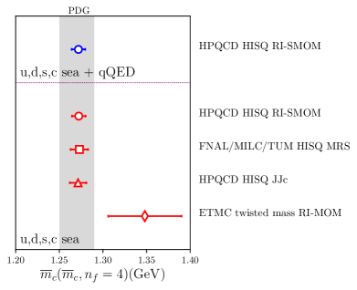
Figure 13: Comparison of lattice QCD results for $m_{c}$ that include $u$, $d$, $s$ and $c$ quarks in the sea. The top two results are the ones from this paper. Our QCD + quenched QED result is given in Eq. (17). Our pure QCD result, Eq. (13), supersedes our earlier result in Lytle et al. (2018). The Fermilab/MILC/TUM result is from Bazavov et al. (2018b) and uses a method based on charm-light meson masses. The ‘HPQCD HISQ JJc’ result is from Chakraborty et al. (2015) and uses current-current correlator techniques. These three results agree to better than 1%. The ETMC result is from Carrasco et al. (2014) and uses the RI-MOM intermediate scheme. The grey band gives the $\pm 1\sigma$ uncertainty band from the Particle Data Group Tanabashi et al. (2018).

Figure 13 gives a comparison of lattice QCD results for $\overline{m}_{c}$. We plot the masses at the scale of the mass, as is conventional even though this is a rather low scale. We restrict the comparison to results that were obtained on gluon field configurations including $u$, $d$, $s$ and $c$ quarks in the sea. The top result is our value from Eq. (17) that explicitly includes a calculation of the impact of quenched QED on the determination of the quark mass.

The top three results in the pure QCD section of the figure all include an estimate of, and correction for, QED effects. These corrections are made, however, by allowing for ‘physical’ QED effects such as those arising from the Coulomb interaction between quark and antiquark in a meson. They do not allow for the QED self-energy contribution which is substantial. Although a large part of this is cancelled by the impact of QED on the mass renormalisation, a consistent calculation has to include both effects, as we have done here.

An important point about Figure 13 is that the top three pure QCD results all have uncertainties of less than 1% and agree to better than 1%, using completely different methods. This implies a smaller uncertainty on $\overline{m}_{c}$ than the 1.5% allowed for by the Particle Data Group Tanabashi et al. (2018). This impressive agreement is not changed by our new result including quenched QED because, as we have shown, the impact of this is at the 0.2% level.

V $J/\psi$ and $\eta_{c}$ decay constants

The decay constant of the $J/\psi$, $f_{J/\psi}$, is defined from the matrix element between the vacuum and a $J/\psi$ meson at rest by

$$\langle 0|\overline{\psi}\gamma_{\mu}\psi|J/\psi\rangle=f_{J/\psi}M_{J/\psi}\epsilon_{\mu},$$ (19)

where $\epsilon_{\mu}$ is the component of the polarisation of the $J/\psi$ in the direction of the vector current. In terms of the ground state amplitude, $A_{0}^{V}$, and mass, $M_{0}^{V}$ ($\equiv E_{0}^{V}$), obtained from the fit of Eq. (3) to the charmonium vector correlator it is (in lattice units)

$$f_{J/\psi}=Z_{V}\sqrt{\frac{2A_{0}^{V}}{M_{0}^{V}}}.$$ (20)

$Z_{V}$ is the renormalisation factor required to match the lattice vector current to that in continuum QCD if a nonconserved lattice vector current is used (as here). We discuss the renormalisation of vector currents using intermediate momentum-subtraction schemes in Hatton et al. (2019) and we will make use of the results based on the RI-SMOM scheme here (see Section II). Note that there is no additional renormalisation required to get from the RI-SMOM scheme to $\overline{\text{MS}}$ because the RI-SMOM scheme satisfies the Ward-Takahashi identity Hatton et al. (2019).

The partial decay width of the $J/\psi$ to an $\ell^{+}\ell^{-}$ pair ($\ell=e,\mu$) is directly related to the decay constant. At leading order in $\alpha_{\mathrm{QED}}$ and ignoring $(m_{\ell}/M_{J/\psi})^{4}$ correction terms, the relation is

$$\Gamma(J/\psi\to\ell^{+}\ell^{-})=\frac{4\pi}{3}\alpha^{2}_{\mathrm{QED,eff}}(M^{2}_{J/\psi})Q_{c}^{2}\frac{f_{J/\psi}^{2}}{M_{J/\psi}},$$ (21)

where $Q_{c}$ is the electric charge of the charm quark in units of the charge of the proton. Note that the formula contains the effective coupling, $\alpha_{\mathrm{QED,eff}}$ evaluated at the scale of $M_{J/\psi}$ but without including the effect of the $J/\psi$ resonance in the running of $\alpha_{\mathrm{QED}}$ to avoid double-counting Keshavarzi et al. (2018).

Experimental values of $\Gamma(J/\psi\to e^{+}e^{-})$ are obtained by mapping out the cross-section for $e^{+}e^{-}\to e^{+}e^{-}$ and $e^{+}e^{-}\to$ hadrons through the resonance region Anashin et al. (2018) or by using initial-state radiation to map out this region via $e^{+}e^{-}\rightarrow\mu^{+}\mu^{-}\gamma$ Ablikim et al. (2016). In either case initial-state radiation and non-resonant background must be taken care of Anashin et al. (2012); Alexander et al. (1989). A cross-section fully inclusive of final-state radiation is obtained; interference between initial and final-state radiation is heavily suppressed Fadin et al. (1994). The resonance parameter determined by the experiment is then the ‘full’ partial width Alexander et al. (1989); Anashin et al. (2010),

$$\Gamma_{\ell\ell}=\frac{\Gamma_{\ell\ell}^{(0)}}{|1-\Pi_{0}|^{2}}$$ (22)

where $\Gamma^{(0)}$ is the partial width to lowest order in QED and $\Pi_{0}$ is the photon vacuum polarisation. The effect of the vacuum polarisation is simply to replace $\alpha_{\mathrm{QED}}$ in the lowest-order QED formula for the width with $\alpha_{\mathrm{QED,eff}}(M^{2})$, as we have done in Eq. (21).

The experimental determination of $\Gamma_{\ell\ell}$ is accurate to 2% for the $J/\psi$ Tanabashi et al. (2018). This allows us to infer a decay constant value from experiment, accurate to 1%, using Eq. (21).

$$f_{J/\psi}^{\mathrm{expt}} = \left(\frac{3M_{J/\psi}}{4\pi Q_{c}^{2}}\right)^{1/2}\frac{\Gamma^{1/2}_{e^{+}e^{-}}}{\alpha_{\mathrm{QED,eff}}}$$

$$= 40.786(\mathrm{MeV})^{1/2}\frac{\Gamma^{1/2}_{e^{+}e^{-}}}{\alpha_{\mathrm{QED,eff}}}\,.$$

Using the experimental average of $\Gamma_{e^{+}e^{-}}=$ 5.53(10) keV Tanabashi et al. (2018), and $\alpha_{\mathrm{QED,eff}}(M^{2}_{J/\psi})=1/134.02(3)$ Keshavarzi et al. (2020) gives

$$f_{J/\psi}^{\mathrm{expt}}=406.5(3.7)(0.5)\,\mathrm{MeV}.$$ (24)

The first uncertainty comes from the experimental uncertainty in $\Gamma$ and the second is an $\mathcal{O}(\alpha_{\mathrm{QED}}/\pi)$ uncertainty for higher-order in QED terms, for example from final-state radiation, in the connection between $\Gamma$ and $f$ in Eq. (21). Note that using $\alpha_{\mathrm{QED}}$ of 1/137 would increase this number by 2.3% (9 MeV).

This experimental value can then be compared to our lattice QCD results for a precision test of QCD. Here we improve on HPQCD’s earlier calculation Donald et al. (2012) by working on gluon field configurations that cover a wider range of lattice spacing values and with sea $u/d$ quark masses now down to their physical values. In addition we now include $c$ quarks in the sea and have a more accurate determination of the vector renormalisation factor $Z_{V}$ Hatton et al. (2019). We will also test the impact on $f_{J/\psi}$ of the $c$ quark’s electric charge.

The decay constant of the pseudoscalar $\eta_{c}$ meson is determined from our pseudoscalar correlators (of spin-taste $\gamma_{5}\otimes\gamma_{5}$) using the ground-state mass and amplitude parameters from the correlator fit, Eq. (2):

$$f_{\eta_{c}}=2m_{c}\sqrt{\frac{2A_{0}^{P}}{(M_{0}^{P})^{3}}}.$$ (25)

Note that this is absolutely normalised and no $Z$ factor is required. Because the $\eta_{c}$ does not annihilate to a single particle there is no experimental process from which we can directly determine $f_{\eta_{c}}$. Nevertheless it is a useful quantity to calculate for comparison to $f_{J/\psi}$ and to fill out the picture of these hadronic parameters from lattice QCD Colquhoun et al. (2015). Again we will improve on HPQCD’s earlier calculation Davies et al. (2010) as discussed above for the $J/\psi$.

V.1 Pure QCD

Table 9: Columns 2 and 3 give the results in lattice units for the $J/\psi$ and $\eta_{c}$ decay constants respectively in pure QCD on the ensembles listed in Table 1. The values of $am_{c}^{\mathrm{val}}$ are those given in Table 1 except for two cases with a deliberately mistuned $c$ quark mass: set 6 denoted by a * where $am_{c}=0.643$ and set 14 denoted by a ${\dagger}$ where $am_{c}$=0.188. The results for $f_{J/\psi}$ do not include the multiplication by $Z_{V}$ needed to normalise them (Eq. (20)). Columns 4 and 5 give the electromagnetic corrections for the $J/\psi$ and $\eta_{c}$ decay constants, as the ratio of the QCD+QED result to that in pure QCD. Again, the electromagnetic corrections for $f_{J/\psi}$ do not include the corrections to $Z_{V}$. $Z_{V}$ values are given in Table 10.

Set	$af_{J/\psi}/Z_{V}$	$af_{\eta_{c}}$	$R^{0}_{\mathrm{QED}}[f_{J/\psi}/Z_{V}]$	$R^{0}_{\mathrm{QED}}[f_{\eta_{c}}]$
1	0.43370(55)	0.37659(18)	-	-
2	0.42346(48)	0.370332(91)	1.00410(64)	1.00294(50)
3	0.4163(11)	0.366127(57)	-	-
4	0.29411(21)	0.268331(61)	-	-
6	0.28835(15)	0.263727(60)	1.00341(37)	1.00326(13)
$6^{*}$	0.28671(15)	0.262077(48)	-	-
8	0.285592(88)	0.261676(26)	-	-
9	0.19406(30)	0.18191(12)	-	-
10	0.191341(79)	0.179362(26)	1.00295(12)	1.002951(54)
11	0.18961(15)	0.178039(24)	-	-
12	0.12334(10)	0.117535(28)	1.00283(33)	1.00311(47)
13	0.119606(63)	0.114151(26)	-	-
14	0.091380(85)	0.087772(39)	-	-
$14^{{\dagger}}$	0.09069(29)	0.086774(59)	-	-

Table 10: Vector current renormalistion constants, $Z_{V}(\mu)$, using the RI-SMOM scheme at $\mu=$ 2 GeV (column 2) and $\mu=$ 3 GeV (column 3) in pure QCD for each $\beta$ value corresponding to a group of ensembles in Table 1. Column 4 gives the QED correction to $Z_{V}$ at 2 GeV in the form of the ratio of the QCD+QED value to that of pure QCD. Most of these values are taken from Hatton et al. (2019) although the $Z_{V}$ value at $\beta=7$ and the QED correction at $\beta=5.8$ are new here.

$\beta$	$Z_{V}$(2 GeV)	$Z_{V}$(3 GeV)	$R_{\mathrm{QED}}[Z_{V}(2\,\mathrm{GeV})]$
5.80	0.95932(18)	-	0.999544(14)
6.00	0.97255(22)	0.964328(75)	0.999631(24)
6.30	0.98445(11)	0.977214(35)	0.999756(32)
6.72	0.99090(36)	0.98702(11)	0.999831(43)
7.00	0.99203(108)	0.99023(56)	-

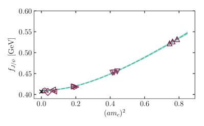
Figure 14: The $J/\psi$ decay constant calculated on the ensembles of Table 1 in pure QCD and plotted against the square of the bare $c$ quark mass in lattice units. The different red shapes correspond to different groups of ensembles with similar lattice spacing and the error bars shown include the full uncertainty on the points. Points at mistuned $m_{c}$ are not plotted but are included in the fit. The green curve marks our extrapolation to the physical point, where the black cross shows the result determined from the experimental average for $\Gamma_{e^{+}e^{-}}$ from Eq. (24).

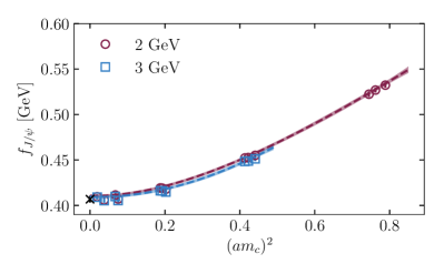
Figure 15: The continuum extrapolation of $f_{J/\psi}$ using $Z_{V}$(2 GeV) (results and fit curve in red, same values as in Fig. 14) and $Z_{V}$(3 GeV) (results and fit curve in blue). The continum extrapolated results agree in the two cases as they should. A black cross shows the experimental average result from Eq. (24).

The second column of Table 9 gives our results for the (unnormalised) values of $af_{J/\psi}$ in pure QCD on 12 of the sets from Table 1. We multiply $af_{J/\psi}/Z_{V}$ by the value of $Z_{V}$ and convert to physical units using the inverse lattice spacing. $Z_{V}$ values are taken from Hatton et al. (2019) except for a new value calculated here for $\beta=7.0$ (ultrafine) set 14. We collect these values in Table 10. See Appendix A for a discussion of the $Z_{V}$ results. The $Z_{V}$ values are very precise and so have little impact on the uncertainty in $f_{J/\psi}$.

Our results for $f_{J/\psi}$ for the pure QCD case are shown in Fig. 14 plotted against the square of the lattice spacing (in units of the bare $c$ quark mass). Clear dependence on the lattice spacing is seen. This dependence comes from the amplitudes of the two-point correlators; the lattice spacing dependence of $Z_{V}$ contributes very little to it. We also plot in Fig. 14 the results of the fit using Eq. (II.6). The priors for the fit are as given in Section II.6 with the prior on the physical value of $f_{J/\psi}$ (i.e. $x$ in Eq. (II.6)) of 0.4(1). The $\chi^{2}/\mathrm{dof}$ of the fit is 0.43. The agreement with the result derived from experiment can clearly be seen. We obtain an $f_{J/\psi}$ value in pure QCD of

$$f_{J/\psi,\mathrm{QCD}}=409.6(1.6)\,\mathrm{MeV}.$$ (26)

We will discuss this result further in Section V.3.

We have used vector current renormalisation factors, $Z_{V}$, in the RI-SMOM scheme at a scale of 2 GeV. The $\mu$ dependence of $Z_{V}$ should just be the result of discretisation effects and results for the physical quantity, $f_{J/\psi}$, using different renormalisation scales $\mu$ should agree in the continuum limit. Here we verify that this is the case using $Z_{V}(2\,\mathrm{GeV})$ and $Z_{V}(3\,\mathrm{GeV})$ results from Table 10 Hatton et al. (2019). There is no 3 GeV result on the very coarse lattices since $\mu a$ would be too large. The comparison for $f_{J/\psi}$ using $\mu$=2 and 3 GeV is shown in Fig. 15 for the pure QCD case. The difference between the two values of $\mu$ is barely visible. The values at $\mu=$ 3 GeV give a continuum limit result of $f_{J/\psi}=$ 408.7(1.8) MeV, in good agreement with that at $\mu=$ 2 GeV in Eq. (26) but slightly less accurate. The $\chi^{2}/\mathrm{dof}$ of the fit was 0.45.

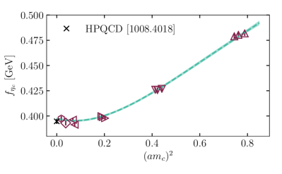
Figure 16: The $\eta_{c}$ decay constant calculated on the ensembles of Table 1 in pure QCD and plotted against the square of the bare $c$ quark mass in lattice units. The different red shapes correspond to different groups of gluon field ensembles with similar lattice spacing. The error bars on each point are the full uncertainty, including correlated uncertainties from, for example, the determination of the lattice spacing. The green curve shows our fit and extrapolation to the physical point. The black cross gives the earlier HPQCD result on $n_{f}=2+1$ gluon field configurations from Davies et al. (2010).

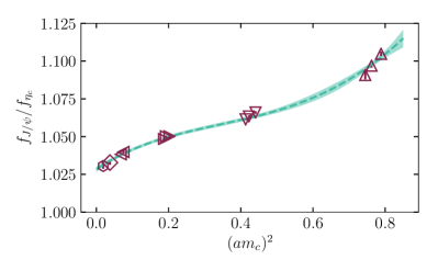
Figure 17: The ratio of $J/\psi$ to $\eta_{c}$ decay constant determined in pure QCD, plotted against the square of the bare $c$ quark mass in lattice units. The different red shapes correspond to different groups of gluon field ensembles with similar lattice spacing. The error bars on each point are the full uncertainty, including correlated uncertainties from, for example, the determination of the lattice spacing. The green curve shows our fit and extrapolation to the physical point.

Our results for $af_{\eta_{c}}$, the $\eta_{c}$ decay constant in lattice units, are given in the third column of Table 9 for the pure QCD case. After conversion to physical units, they are plotted in Figure 16. The curve is similar to that for $f_{J/\psi}$ but with somewhat smaller discretisation effects. We also plot the results of performing the same fit as for $f_{J/\psi}$ using Eq. (II.6). The $\chi^{2}/\mathrm{dof}$ of the fit is 0.88 giving a result for the decay constant in pure QCD of

$$f_{\eta_{c},\mathrm{QCD}}=397.5(1.0)\,\mathrm{MeV}.$$ (27)

This agrees well with the earlier HPQCD value on $n_{f}=2+1$ gluon field configurations Davies et al. (2010) of 0.3947(24) GeV but has half the uncertainty. In Davies et al. (2010) the effects from neglecting the charm quark in the sea are estimated to be $\mathcal{O}(0.01\%)$ which is negligible and means that the two calculations should give the same result.

Figure 17 shows our results for the ratio of $f_{J/\psi}$ to $f_{\eta_{c}}$ in pure QCD. A lot of the discretisation effects cancel in the ratio, as is evident in comparing this figure to Figures 14 and 16. Systematic uncertainties, for example from the determination of the lattice spacing, are also reduced. The shape of the curve again, as in the hyperfine splitting case, reflects the fact that we have successfully reduced sources of $a^{2}$ error to the point where $a^{4}$ and $a^{6}$ are visible.

We fit the ratio to the same fit as before (Eq. (II.6)) with a prior on the physical value of 1.0(1). The fit has a $\chi^{2}/\mathrm{dof}$ of 0.62 and returns a physical value for the decay constant ratio in pure QCD of

$$\frac{f_{J/\psi,\mathrm{QCD}}}{f_{\eta_{c},\mathrm{QCD}}}=1.0285(18).$$ (28)

Thus we see that the $J/\psi$ decay constant is nearly 3% larger than that of the $\eta_{c}$ with an uncertainty of 0.2%.

Table 11: Error budget for the $J/\psi$ and $\eta_{c}$ decay constants as a percentage of the final answer.

	$f_{J/\psi}$	$f_{\eta_{c}}$
$a^{2}\to 0$	0.09	0.03
$Z_{V}$	0.05	-
Pure QCD Statistics	0.12	0.05
QCD+QED Statistics	0.05	0.02
$w_{0}/a$	0.11	0.08
$w_{0}$	0.34	0.24
Valence mistuning	0.05	0.01
Sea mistuning	0.01	0.00
Total	0.40%	0.26%

Table 11 gives the error budget for our final values of $f_{J/\psi}$ and $f_{\eta_{c}}$, both for the pure QCD case and the QCD+QED case to be discussed in Section V.2. The contributions from different sources are very similar between the two decay constants. It is clear from this that the dominant sources of error are related to the determination of the lattice spacing, as for the hyperfine splitting.

The error budget presented here for the $J/\psi$ decay constant is markedly different from that of Donald et al. (2012). There the dominant contribution to the error was from the vector renormalisation constant, $Z_{V}$, obtained using a matching between lattice time moments and high order perturbative QCD Kuhn et al. (2007). Here that error is substantially reduced by using the $Z_{V}$ values obtained in lattice QCD fully nonperturbatively in the RI-SMOM scheme Hatton et al. (2019). Note that the uncertainty from scale-setting in the decay constant is much smaller than that for the hyperfine splitting (Table 5). This is because the decay constant has opposite behaviour as a function of quark mass, increasing as the quark mass increases rather than decreasing. This then offsets, rather than augments (as in the hyperfine splitting case), its sensitivity to changes in the scale-setting parameter, $w_{0}$.

V.2 Impact of Quenched QED

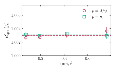
Figure 18: The fractional QED correction to the $J/\psi$ and $\eta_{c}$ decay constants as a function of lattice spacing. The horizontal dashed lines mark the weighted average of the points.

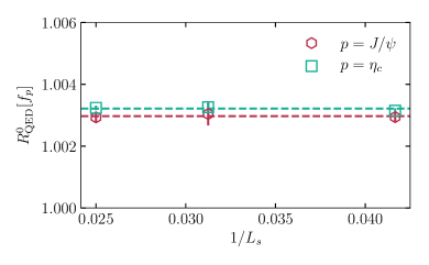
Figure 19: The volume dependence of the fractional QED effect on the $J/\psi$ and $\eta_{c}$ decay constants measured on sets 5-7. The dashed lines are horizontal and indicate the weighted average of the points. There is no observable finite volume effect at the level of our statistical uncertainties.

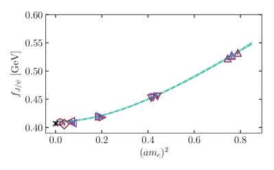
Figure 20: The $J/\psi$ decay constant calculated on the ensembles of Table 1 in pure QCD (red points) and including also quenched QED (blue points) plotted against the square of the bare $c$ quark mass in lattice units. The green curve marks our extrapolation to the physical point, where the black cross shows the experimental average result from Eq. (24).

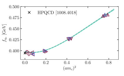
Figure 21: The $\eta_{c}$ decay constant calculated on the ensembles of Table 1 in pure QCD (red points) and including also quenched QED (blue points) plotted against the square of the bare $c$ quark mass in lattice units. The green curve marks our extrapolation to the physical point. The black cross gives the earlier HPQCD result on $n_{f}=2+1$ gluon field configurations from Davies et al. (2010).

Including quenched QED effects into our calculations allows us to determine the effect on the $J/\psi$ and $\eta_{c}$ decay constants of the electric charge of the valence $c$ quarks. Because the $J/\psi$ and $\eta_{c}$ are electrically neutral particles, there is no long-distance infrared component to cause problems (as there is for $f_{\pi^{+}}$) and we can simply proceed to determine the decay constants after the addition of the QED field as we did in the pure QCD case.

The fractional QED effect on the $J/\psi$ and $\eta_{c}$ decay constants at fixed bare $c$ quark mass in lattice units is given in Table 9. We see a 0.3% increase, offset slightly by the change in $Z_{V}$ in the $J/\psi$ case. The fractional QED effect on $Z_{V}$ is given in Table 10. The fractional QED effect at fixed bare mass is plotted in Figure 18. We see that the effect is similar for the $J/\psi$ and $\eta_{c}$ in the continuum limit and shows very little dependence on the lattice spacing.

The volume dependence of the fractional QED effect is shown in Figure 19 on sets 5–7. We find that the effect is negligible well below the 0.1% level.

We now combine our QCD+QED results with our pure QCD results and the full fit of Eq. (II.6), which takes into account the retuning of the quark mass needed when quenched QED is included. Figure 20 shows our pure QCD results, QCD+QED results and fit curve for the $J/\psi$ decay constant. We obtain

$$f_{J/\psi,\mathrm{QCD+QED}}=410.4(1.7)\,\mathrm{MeV}.$$ (29)

This is a 0.2% increase over the value in pure QCD (Eq. (26)) because retuning reduces the quark mass and offsets some of the impact of quenched QED seen in Table 9. A more accurate statement is that the final fractional effect from quenched QED is $R_{\mathrm{QED}}[f_{J/\psi}]=$1.00188(36).

A very similar picture is seen for $f_{\eta_{c}}$ in Figure 21. We obtain

$$f_{\eta_{c},\mathrm{QCD+QED}}=398.1(1.0)\,\mathrm{MeV}.$$ (30)

The final fractional effect from quenched QED is then $R_{\mathrm{QED}}[f_{\eta_{c}}]=$1.00166(25).

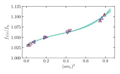
Figure 22: The ratio of $J/\psi$ to $\eta_{c}$ decay constants calculated on the ensembles of Table 1 in pure QCD (red points) and including also quenched QED (blue points) plotted against the square of the bare $c$ quark mass in lattice units. The green curve marks our extrapolation to the physical point.

Finally, in Figure 22 we plot results for the ratio of $J/\psi$ to $\eta_{c}$ decay constants and show the fit curve extrapolated to the continuum limit. This gives

$$\frac{f_{J/\psi,\mathrm{QCD+QED}}}{f_{\eta_{c},\mathrm{QCD+QED}}}=1.0284(19).$$ (31)

This is almost the same as the pure QCD result.

V.3 Discussion : $f_{J/\psi}$ and $f_{\eta_{c}}$

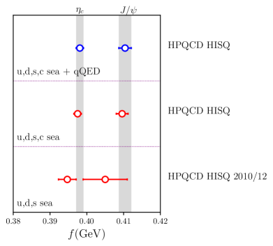
Figure 23: A comparison of our new results for $f_{\eta_{c}}$ and $f_{J/\psi}$ with earlier lattice QCD results, also by HPQCD, on gluon field configurations that include $n_{f}=2+1$ flavours of quarks in the sea. The results labelled ‘HPQCD HISQ’ are from this paper and the results labelled ‘HPQCD HISQ 2010/12’ are from Davies et al. (2010); Donald et al. (2012). The grey bands are the $\pm 1\sigma$ bands from our new QCD+QED results.

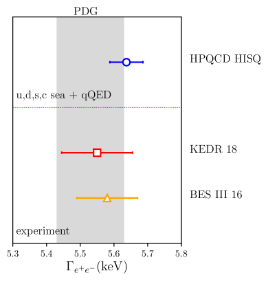
Figure 24: A comparison of the width for $J/\psi$ decay to $e^{+}e^{-}$ implied by our new results for $f_{J/\psi}$ to that obtained from two recent experiments. The point labelled ‘KEDR 18’ is from Anashin et al. (2018) and the point labelled ‘BES III 16’ is from Ablikim et al. (2016). The grey bands are the $\pm 1\sigma$ bands from the Particle Data Group average Tanabashi et al. (2018).

Figure 23 compares our new pure QCD and QCD+QED results to previous results including $n_{f}=2+1$ flavours of sea quarks for $f_{\eta_{c}}$ Davies et al. (2010) and $f_{J/\psi}$ Donald et al. (2012). There is good agreement. These earlier calculations also used HISQ quarks but our new results are more accurate, particularly for $f_{J/\psi}$ because of the use of more accurate values of $Z_{V}$ Hatton et al. (2019).

There have also been calculations that use $n_{f}=2$ flavours of sea quarks. It is harder to make a comparison to these results because it is not clear what the systematic error is from not including at least the $s$ quarks in the sea, and no uncertainty is included for this. The calculation of Bečirević et al. (2014) uses twisted-mass quarks on $n_{f}=2$ gluon field configurations and obtains $f_{\eta_{c}}=$387(7)(2) MeV and $f_{J/\psi}=$418(8)(5) MeV. The calculation of Bailas et al. (2018) uses clover quarks on $n_{f}=2$ CLS gluon-field configurations to give $f_{\eta_{c}}=$387(3)(3) MeV and $f_{J/\psi}=$399(4)(2) MeV. The $n_{f}=2$ results for $f_{\eta_{c}}$ agree with each other and have a central value about 2$\sigma$ below ours. The $\sigma$ here is that from the $n_{f}=2$ results since our uncertainty is much smaller. The $n_{f}=2$ results for $f_{J/\psi}$ are compatible with each other and with our result, again at $2\sigma$.

As discussed in Section V, the $J/\psi$ decay constant is the hadronic quantity that is needed to determine the rate of $J/\psi$ annihilation to leptons via Eq. (21). Our result for $\Gamma$ using Eq. (21) with $f_{J/\psi}$ from Eq. (29) is

$$\Gamma(J/\psi\rightarrow e^{+}e^{-})=5.637(47)(13)\,\mathrm{keV}.$$ (32)

The first uncertainty is from our lattice QCD+QED result for $f_{J/\psi}$ and the second uncertainty allows for a relative $\mathcal{O}(\alpha_{\mathrm{QED}}/\pi)$ correction to Eq. (21) from higher-order effects.

Figure 24 compares this width $\Gamma(J/\psi\rightarrow e^{+}e^{-})$ to results from experiment. Recent experimental results from KEDR Anashin et al. (2018) and BES III Ablikim et al. (2016) are shown along with the Particle Data Group average Tanabashi et al. (2018) (as a grey band). Figure 24 shows good agreement between our result and the experimental values shown, as well as the experimental average.

The lattice QCD result is now more accurate than the experimental values.

VI Vector correlator moments and $a_{\mu}^{c}$

Table 12: Time-moments of charmonium vector current-current correlators calculated on the ensembles in Table 1. The results tabulated are values of $(G_{n}/Z_{V}^{2})^{1/(n-2)}$ in lattice units along with their statistical uncertainties, given for $n=4$, 6, 8 and 10 in columns 2, 3, 4 and 5. Uncertainties are statistical only. Note that the results for different moments are correlated because they are determined from the same correlation functions. The results marked with a $*$ and ${\dagger}$ are for deliberately mistuned $am_{c}$ values as detailed in the caption to Table 3. Also included are the ratios at fixed $am_{c}$, denoted $R^{0}_{\mathrm{QED}}$, of QCD+QED to QCD results for each rooted moment on a subset of ensembles.

Set	$n=4$	$n=6$	$n=8$	$n=10$	$R_{\mathrm{QED}}^{0}[n=4]$	$R_{\mathrm{QED}}^{0}[n=6]$	$R_{\mathrm{QED}}^{0}[n=8]$	$R_{\mathrm{QED}}^{0}[n=10]$
1	0.389670(40)	0.949791(62)	1.410524(75)	1.815497(88)	-	-	-	-
2	0.396283(22)	0.961260(35)	1.425498(42)	1.833868(49)	0.999954(26)	0.999910(17)	0.999858(15)	0.999810(15)
3	0.400779(15)	0.969045(24)	1.435671(28)	1.846369(33)	-	-	-	-
4	0.511194(12)	1.164351(19)	1.701040(26)	2.184698(34)	-	-	-	-
6	0.5206344(85)	1.181180(14)	1.724311(19)	2.214708(24)	0.9998455(15)	0.9997169(11)	0.9995987(10)	0.9994908(11)
$6^{*}$	0.5254224(87)	1.189687(14)	1.736041(19)	2.229780(25)	-	-	-	-
8	0.5254560(47)	1.1897785(76)	1.736217(10)	2.230069(13)	-	-	-	-
9	0.70981(13)	1.53941(21)	2.24688(27)	2.90799(32)	-	-	-	-
10	0.723760(11)	1.566115(20)	2.285959(27)	2.959283(36)	0.999554(24)	0.999312(20)	0.999124(20)	0.998995(22)
11	0.731489(11)	1.580936(18)	2.307649(25)	2.987715(32)	-	-	-	-
12	1.070736(33)	2.276543(58)	3.355470(80)	4.37418(10)	0.999096(59)	0.998767(49)	0.998584(48)	0.998489(48)
13	1.114660(44)	2.366266(78)	3.48827(11)	4.54699(14)	-	-	-	-
14	1.431378(91)	3.03675(16)	4.49434(22)	5.86769(29)	-	-	-	-
$14^{\dagger}$	1.46556(17)	3.10710(31)	4.59734(43)	6.00058(56)	-	-	-	-
15	1.91475(23)	4.06357(42)	6.02429(55)	7.86806(66)	-	-	-	-

With new results expected from the Fermilab $g-2$ experiment soon there has been a concerted effort by the lattice community to understand and control systematic effects in the lattice QCD calculation of the hadronic vacuum polarisation (HVP) contribution to the anomalous magnetic moment of the muon. Since the most accurate values for the HVP currently come from experimental results on $R(e^{+}e^{-}\rightarrow\mathrm{hadrons})$, it is also important to compare lattice QCD results to these, disaggregated by flavour where possible.

The first calculation of the quark-line connected $c$-quark contribution to the HVP, $a_{\mu}^{c}$, was given in Chakraborty et al. (2014) using results for the time-moments of vector charmonium current-current correlators calculated in Donald et al. (2012). The time moments are defined by

$$G_{n}=Z_{V}^{2}\sum_{t}t^{n}C_{V}(t),$$ (33)

where $C_{V}(t)$ is the vector current-current correlator and $Z_{V}$ is the vector current renormalisation factor, discussed in Section V. Note that $t\in\{-L/2+1,-L/2+2,\ldots,L/2\}$.

The even-in-$n$ time-moments for $n\geq 4$ can be related to the derivatives at $q^{2}=0$ of the renormalised vacuum polarisation function Allison et al. (2008), $\hat{\Pi}(q^{2})\equiv\Pi(q^{2})-\Pi(0)$, by

$$G_{n}=\left.(-1)^{n/2}\frac{\partial^{n}}{\partial q^{n}}q^{2}\hat{\Pi}(q^{2})\right|_{q^{2}=0}.$$ (34)

This means that $\hat{\Pi}(q^{2})$ can be reconstructed, using Padé approximants, from the $G_{n}$ Chakraborty et al. (2014) and fed into the integral over $q^{2}$ that yields the quark-line connected HVP contribution to $a_{\mu}$ Blum (2003). Only time-moments of low moment number are needed to give an accurate result for $a_{\mu}^{c}$ because the integrand is dominated by small $q^{2}$. We will give results for the four lowest moments, $n={4,6,8,10}$, improving on the values given in Donald et al. (2012). The improvement comes mainly through the use of a more accurate vector current renormalisation as well as an improved method for reducing lattice spacing uncertainties but we also use second-generation gluon field configurations that include $c$ quarks in the sea and calculate, rather than estimate, the impact of the leading QED effects.

$\hat{\Pi}(q^{2})$ and hence $a_{\mu}^{c}$ can also be determined from experimental results for $R_{c}\equiv R(e^{+}e^{-}\rightarrow c\overline{c}\rightarrow\mathrm{hadrons})$ as a function of squared centre-of-mass energy, $s$. This can be done using inverse-$s$ moments

$$\mathcal{M}_{k}\equiv\int\frac{ds}{s^{k+1}}R_{c}(s)\,.$$ (35)

$R_{c}$ is obtained from the full $e^{+}e^{-}$ rate from just below the $c$ threshold upwards by subtracting the background contribution from $u$, $d$, and $s$ quarks perturbatively, see e.g. Kuhn et al. (2007).

The relationship between $G_{2k+2}$ and $\mathcal{M}_{k}$ is then

$$G_{2k+2}=\frac{(2k+2)!\mathcal{M}_{k}}{12\pi^{2}Q^{2}}.$$ (36)

A comparison of our correlator time-moments calculated on the lattice and extrapolated to the continuum limit to the inverse-$s$ moments determined from experiment is equivalent to a test of the agreement of the results for $a_{\mu}^{c}$ in the two cases.

VI.1 Vector correlator moments: Pure QCD and QCD+QED results

Table 12 gives our raw results for the time-moments of the same vector current-current correlators from which we have determined the mass and decay constant of the $J/\psi$ meson in Sections III and V. Notice that the statistical uncertainties are tiny. The correlators make use of a local vector current that must be renormalised as discussed in Section V. The results in Table 12 are calculated before renormalisation and are given in lattice units. The quantity that is tabulated is

$$\left(\frac{G_{n}}{Z_{V}^{2}}\right)^{1/(n-2)}\,.$$ (37)

We take the $(n-2)$th root to reduce all results to the same dimensions Donald et al. (2012). To normalise the time-moments we use the $Z_{V}$ values at $\mu$= 2 GeV given in Table 10 that were used for $f_{J/\psi}$ in Section V.

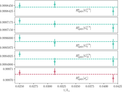
Figure 25: A study of the volume dependence of the electromagnetic correction to the first four time moments of the vector current-current correlator and to $a_{\mu}^{c}$ on sets 5-7. There is no observable dependence on the lattice spatial extent, $L_{s}$, as can be judged by comparison to the dashed horizontal lines at the weighted averages of the points.

Table 12 also gives the result of including quenched QED as the ratios $R^{0}_{\mathrm{QED}}$ for each rooted moment (at fixed $am_{c}$). These values are all very slightly less than 1, by up to 0.1% for $n$=4, and 0.2% for $n$=10. We can also test the finite-volume dependence of the quenched QED effect using sets 5, 7 and 8 and the results are shown in Fig. 25. There is no visible volume dependence in the QED effect on time-moments at the level of our statistical uncertainties. This is to be expected, as seen for the $J/\psi$ mass and decay constant in Sections III and V, since the vector current being used here is electrically neutral.

To fit the results as a function of lattice spacing it is convenient to work with the dimensionless combination:

$$M_{J/\psi}\left(G_{n}\right)^{1/(n-2)}\,,$$ (38)

using our $M_{J/\psi}$ masses from Table 3. The removal of dimensions reduces the uncertainty coming from the value of the lattice spacing. At the same time this quantity also has reduced sensitivity to mistuning of the valence $c$ quark mass because the $m_{c}$-dependence is largely cancelled by $M_{J/\psi}$. We fit the quantity defined in Eq. (38) as a function of lattice spacing, allowing for quark-mass mistuning effects of both valence and sea quarks to derive results in the physical continuum limit. We do this as before using the fit function given in Eq. (II.6). Values in the physical continuum limit are then divided by $M_{J/\psi}$ from experiment to obtain our final results for $G_{n}^{1/(n-2)}$ in $\mathrm{GeV}^{-1}$. In doing this we allow an uncertainty of 0.7 MeV in $M_{J/\psi}$ from annihilation to a photon (see Section III) since this effect is not included in our results.

Table 13: QCD+QED results in the physical continuum limit for the first four time-moments (column 2) compared with the results extracted from experiment in column 3 Dehnadi et al. (2013). Agreement within 2$\sigma$ is seen for all except the 4th moment, but the lattice QCD results are much more accurate. Column 4 gives the effect of quenched QED as a ratio of the physical results in QCD+QED to those in pure QCD.

$n$	$G_{n}^{1/(n-2)}$	$(G_{n}^{\mathrm{exp.}})^{1/(n-2)}$	$R_{\mathrm{QED}}[G_{n}^{1/(n-2)}]$
	$\mathrm{GeV}^{-1}$	$\mathrm{GeV}^{-1}$	$-$
4	0.31715(49)	0.3110(26)	1.00106(13)
6	0.67547(84)	0.6705(31)	1.00069(11)
8	1.0041(11)	0.9996(36)	1.00047(10)
10	1.3117(13)	1.3080(37)	1.00037(10)

Fig. 26 plots the results for the rooted moments multiplied by $M_{J/\psi}$ as a function of $(am_{c})^{2}$. Also shown is the fit result from Eq. (II.6). Only the pure QCD lattice results are shown for clarity; those including the effect of quenched QED are very close to them. The fit result plotted is that for the QCD+QED case.

Table 13 gives our QCD+QED results for the 4th, 6th, 8th and 10th rooted moments in the physical continuum limit. These are obtained from a simultaneous fit to all of the moments, including the correlations between them (since they are derived from the same correlators). The fit has a $\chi^{2}/\mathrm{dof}$ of 0.62 for an svdcut of $1\times 10^{-3}$.

Column 3 of Table 13 gives the results derived from experimental data for $R(e^{+}e^{-}\rightarrow\mathrm{hadrons})$ and $\Gamma_{\ell\ell}$ and mass for the $J/\psi$ and $\psi^{\prime}$ by Dehnadi et al. (2013) for comparison (see Section VI). We have converted these results into the quantity that we calculate according to Eq. (36). We see agreement within 2$\sigma$ for $n\geq 6$ with the values derived from experiment, but a 2.4$\sigma$ tension at $n=4$. The results given from Dehnadi et al. (2013) correspond to their standard selection of experimental datasets. Results shift by $\pm 1\sigma$ for other selections. Note that the lattice QCD results are now much more precise than those determined from experiment. The comparison between lattice QCD and experiment will be discussed further in Section VI.2.

Column 4 of Table 13 gives the final impact of quenched QED, including the quark mass retuning, on the moments. We see that the ratios, $R_{\mathrm{QED}}[G_{n}^{1/(n-2)}]$, are greater than 1, in contrast to the $R^{0}_{\mathrm{QED}}$ of Table 12 that are less than 1. As discussed in Section II.2, the inclusion of QED means that the $c$ quark mass must be retuned downwards. The rooted time-moments are approximately inversely proportional to the quark mass and so they increase under this retuning, more than offsetting the direct effect of QED seen in $R^{0}_{\mathrm{QED}}$.

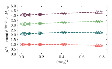
Figure 26: The four lowest time moments and their extrapolation to $a=0$. The symbols give results for the rooted moment multiplied by $M_{J/\psi}$ with different symbols denoting different groups of ensembles with similar lattice spacing. The diffferent colours pick out the different moments, from $n=4$ at the bottom to $n=10$ at the top of the plot. Only the results from the pure QCD calculation at well-tuned $c$ quark masses are shown for clarity. Uncertainties are too small to be visible. The extrapolation for all the moments are performed simultaneously including correlations between moments determined from the same current-current correlators. The dashed lines give the QCD+QED fit curve using Eq. (II.6) and the coloured crosses mark the result in the continuum limit at physical quark masses.

Table 14: Error budget for $G_{n}^{1/(n-2)}$ as a percentage of the final answer.

	$G_{4}^{1/2}$	$G_{6}^{1/4}$	$G_{8}^{1/6}$	$G_{10}^{1/8}$
$a^{2}\to 0$	0.06	0.05	0.04	0.03
$Z_{V}$	0.04	0.02	0.02	0.02
Pure QCD Statistics	0.03	0.02	0.02	0.02
QCD+QED Statistics	0.01	0.01	0.01	0.01
Sea mistunings	0.06	0.03	0.03	0.03
Valence mistunings	0.01	0.00	0.00	0.00
$M_{J/\psi}$	0.02	0.02	0.02	0.02
$w_{0}$	0.10	0.08	0.06	0.05
$w_{0}/a$	0.06	0.05	0.05	0.04
Total	0.15	0.12	0.11	0.10

Table 14 gives the error budget for the $G_{n}$. The total uncertainty in all cases is below 0.2%.

VI.2 Discussion: Vector correlator moments

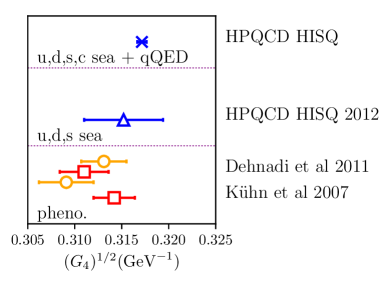
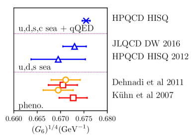
Figure 27: Comparison of our new result to those of previous lattice QCD calculations for the 4th and 6th time-moments (appropriately rooted) of the charmonium vector current-current correlator. Our new result obtained here on $n_{f}=2+1+1$ gluon field configurations and including the effect of quenched QED is given at the top (blue cross). HPQCD’s 2012 result on $n_{f}=2+1$ gluon field configurations with HISQ valence $c$ quarks is marked ‘HPQCD HISQ 2012’ Donald et al. (2012). JLQCD’s 2016 result using $n_{f}=2+1$ domain-wall quarks is marked ‘JLQCD DW 2016’ for the 6th moment only. We also compare to results (open red squares) denoted ‘pheno.’ that are derived from experimental data for the cross-section for $e^{+}e^{-}$ to hadrons as a function of centre-of-mass energy, by determining the $c\overline{c}$ component. The points plotted come from Kuhn et al. (2007) and Dehnadi et al. (2013). Open orange circles show alternative selections of datasets from Dehnadi et al. (2013); the upper value is for the ‘maximal’ set and the lower value for the ‘minimal’ set.

Our new results for the time-moments of vector current-current correlators improve significantly on earlier lattice QCD calculations and are now more accurate than results derived from experiment.

Figure 27 compares our new results for the 4th and 6th moments to earlier lattice QCD results. Comparison for the 8th and 10th moments gives a very similar picture and so is not shown. The first lattice QCD calculation of the time-moments of vector charmonium current-current correlators was given by HPQCD in Donald et al. (2012) using HISQ valence quarks on $n_{f}=2+1$ asqtad gluon field configurations. Our new results have an uncertainty almost ten times smaller than these. The error budget in the earlier results was dominated by the uncertainty in $Z_{V}$ from the use of continuum perturbation theory in the matching factors and there was also a sizeable uncertainty from the lattice spacing. These uncertainties have been enormously reduced here and in addition we no longer need an uncertainty from missing QED effects. We also show a comparison with the subsequent results from the JLQCD collaboration Nakayama et al. (2016) using domain-wall quarks on $n_{f}=2+1$ gluon field configurations. JLQCD do not give a value for the 4th moment because of discretisation effects in their formalism (tree-level $\mathcal{O}(a^{2})$). The dominant uncertainties in their results are from statistics and from the value of $t_{0}^{1/2}$ used to fix the lattice spacing, on which they have a 2% uncertainty. Good agreement is seen for all of the lattice QCD results.

Two of the most recent results from phenomenological determinations of the moments Kuhn et al. (2007); Dehnadi et al. (2013) are also compared in Fig. 27. The results from Dehnadi et al. (2013) include experimental datasets for the inclusive cross-section that are both older and newer than those used in Kuhn et al. (2007). Results from Dehnadi et al. (2013)’s ‘standard’ selection of datasets were given in Table 13 and are shown in Fig. 27 in red. We also show, in orange, the results from the ‘maximal’ set (all experimental information available at that point) and the ‘minimal’ set (datasets that are needed to cover the full $\sqrt{s}$ range from 2 GeV to 10.5 GeV without gaps, keeping the most accurate results). Note that the resonance parameters are the same for all selections. We see that the variation with dataset selection covers almost $1\sigma$ for the 4th moment, but much less for the 6th moment. This is also reflected in the differences between Dehnadi et al. (2013) and Kuhn et al. (2007).

These phenomenological analyses must subtract the ‘non-charm’ background from experimental results for $R(e^{+}e^{-}\rightarrow\mathrm{hadrons})$ to leave $R_{c}$ for Eq. (35). $R_{c}$ is defined to be the result from diagrams with a charm quark loop connected to a photon at both ends Kuhn et al. (2007) i.e. the quark-line connected vector current-current correlator that we study on the lattice. The subtracted background includes QED effects for the non-charm and singlet (quark-line disconnected) contributions. The remainder, $R_{c}$ then includes the QED effects associated with the $c\overline{c}$ loop. The dominant source of uncertainty in $R_{c}$ comes from the charmonium resonance ($J/\psi$ and $\psi^{\prime}$) region and is set by the uncertainty in $\Gamma_{ee}$ for these states. The fractional uncertainty is approximately the same for all moments Kuhn et al. (2007); Dehnadi et al. (2013). When the $(n-2)$th root is taken the fractional uncertainty then falls with increasing $n$.

Good agreement is seen between the phenomenological results and our new lattice results for $n=6$, 8 and 10, although the lattice results are systematically at the upper end of the phenomenological range. The largest discrepancy is a 2.8$\sigma$ tension for the 4th moment between us and the results of Dehnadi et al. (2013) for their minimal selection of datasets. The tension is 2.4$\sigma$ for the standard selection, and below 2$\sigma$ for the maximal selection and for the results of Kuhn et al. (2007). The $\sigma$ here is that for the phenomenological results since the lattice uncertainty is much smaller. Because the 4th moment dominates the determination of $a_{\mu}^{c}$, this tension between lattice QCD+QED and some of the phenomenological results carries over to $a_{\mu}^{c}$, to be discussed in the next section.

The time-moments can also be used to determine a value for $\overline{m}_{c}$ by comparing to $\mathcal{O}(\alpha_{s}^{3})$ continuum QCD perturbation theory and this was the focus of Kuhn et al. (2007); Dehnadi et al. (2013). We do not do this here because the scale of $\alpha_{s}$ is rather low in these determinations meaning that uncertainties from missing higher-order corrections can be substantial. We prefer instead the method of Chakraborty et al. (2015), which enables a higher scale to be used in the perturbation theory. We have checked, however that the $m_{c}$ value that would be obtained from the time-moments is consistent with both Chakraborty et al. (2015) and the value given in Section IV.

VI.3 $a_{\mu}^{c}$: Pure QCD and QCD+QED results

Table 15: Values of $a_{\mu}^{c}$ on the ensembles of Table 1 and the direct quenched QED correction on a subset of those ensembles. Those marked with a $*$ and ${\dagger}$ are at deliberately mistuned $c$ masses (see caption to Table 3). The uncertainties quoted are correlated through the value of $M_{J/\psi}$ (for all ensembles, see text) and $Z_{V}$ (for ensembles at a given $\beta$).

Set	$a_{\mu}^{c}\times 10^{9}$	$R_{\mathrm{QED}}^{0}\left[a_{\mu}^{c}\right]$
1	1.23183(78)	-
2	1.24522(75)	1.000478(80)
3	1.25431(77)	-
3A	1.25518(49)	-
3B	1.25485(48)	-
4	1.40782(91)	-
6	1.41738(91)	1.001080(89)
$6^{*}$	1.42370(91)	-
8	1.42234(91)	-
9	1.47866(97)	-
10	1.48514(75)	1.001416(83)
11	1.48853(75)	-
12	1.4725(13)	1.00141(15)
13	1.4805(13)	-
14	1.4610(33)	-
$14^{\dagger}$	1.4702(33)	-
15	1.4572(10)	-

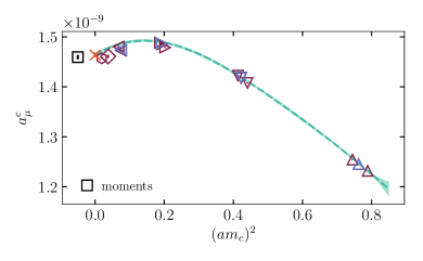
Figure 28: Extrapolation to the continuum physical point of the connected charm HVP contribution to the anomalous magnetic moment of the muon. Different symbols denote results on groups of ensembles with similar lattice spacing. Results at deliberately mistuned $c$ quark masses are not plotted but are included in the fit. The red points correspond to pure QCD, the light blue points to QCD+QED and the dashed green fit curve plotted is that for QCD+QED. The continuum result (red cross) is compared to the result (open black square) obtained by calculating $a_{\mu}^{c}$ from the individually extrapolated time-moments in Section VI.1.

To calculate the quark-line connected HVP contribution to $a_{\mu}$ from $c$ quarks, $a_{\mu}^{c}$, we can either use the physical results for the vector current-current correlator time-moments discussed in the previous subsection or we can calculate $a_{\mu}^{c}$ on each lattice ensemble and perform a fit as a function of lattice spacing to extrapolate directly to the continuum limit. We will do the latter here.

The values of $a_{\mu}^{c}$ on each lattice are given in Table 15. These are determined from the time-moments rescaled by the $J/\psi$ mass on each lattice :

$$\frac{M_{J/\psi}G_{n}^{1/(n-2)}}{M_{J/\psi}^{\mathrm{expt}}}\,.$$ (39)

As discussed in Section VI.1 rescaling by $M_{J/\psi}$ reduces the lattice spacing uncertainty and the impact of mistuning the $c$ quark mass. This was used for lighter quark masses in Chakraborty et al. (2017a) (see also Burger et al. (2014)). The reduced effect of mistuning is clear from comparing the mistuned results in Table 15 to those in Table 12.

Table 15 also includes results on the two ensembles, sets 3A and 3B, that allow direct comparison of the effects of strong-isospin breaking the sea. The ratio of the two results is 0.99974(14), so the results agree to within 0.03% (and 2$\sigma$), consistent with these effects being negligible here (see Section II.4).

Table 15 also gives the direct effect of quenched QED through the ratio $R^{0}_{\mathrm{QED}}[a_{\mu}^{c}]$. Because the rescaled moments have less sensitivity to the $c$ quark mass these numbers are larger than 1 (unlike the results in Table 12) and reflect more closely the final impact of QED on $a_{\mu}^{c}$. We observe no finite-volume dependence for the quenched QED corrections to $a_{\mu}^{c}$, as for the correlator time moments. This is shown in Fig. 25.

The results from Table 15 are shown in Fig. 28 along with our standard fit of the form given in Eq. (II.6). The fit has a $\chi^{2}/\mathrm{dof}$ of 0.44. This fit obtains the physical values

$$a_{\mu}^{c} = 14.606(47)\times 10^{-10},\quad\mathrm{QCD}$$ (40)

$$a_{\mu}^{c} = 14.638(47)\times 10^{-10},\quad\mathrm{QCD+QED}$$

along with $R_{\mathrm{QED}}[a_{\mu}^{c}]=1.00214(19)$. These results agree well (within $1\sigma$) with those obtained using the extrapolated values for the moments from Table 13 and calculating $a_{\mu}^{c}$ in the continuum, as is seen in Fig. 28.

The error budget for our final value of $a_{\mu}^{c}$ is given in Table 16. The largest uncertainties come from the determination of the lattice spacing, although this uncertainty is much reduced by our rescaling with $M_{J/\psi}$.

Table 16: Error budget for $a_{\mu}^{c}$ from our fit to $a_{\mu}^{c}$ values on each ensemble.

	$a_{\mu}^{c}$
$a^{2}\to 0$	0.15
$Z_{V}$	0.07
Pure QCD Statistics	0.08
QCD+QED Statistics	0.01
$w_{0}/a$	0.16
$w_{0}$	0.18
Sea mistunings	0.09
Valence mistunings	0.03
$M_{J/\psi}^{\mathrm{exp.}}$	0.05
Total	0.32

VI.4 Discussion: $a_{\mu}^{c}$

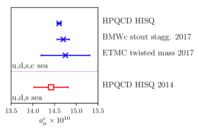
Figure 29: Comparison of lattice QCD results (not including QED) for the connected $c$ quark HVP contribution to $a_{\mu}$, $a_{\mu}^{c}$. Results are divided according to the number of sea quark flavours included in the gluon field configurations on which the calculation was done. The first result, labelled ‘HPQCD HISQ 2014’ is from Chakraborty et al. (2015) using values of time-moments determined in Donald et al. (2012) using HISQ valence quarks on gluon field configurations including $n_{f}=2+1$ flavours of asqtad sea quarks. The other results all include $n_{f}=2+1+1$ flavours of sea quarks. The result labelled ‘ETMC twisted mass 2017’ uses the twisted mass formalism Giusti et al. (2017) and that labelled ‘BMW stout stagg. 2017’ a smeared staggered quark action Borsanyi et al. (2018). Our new result (from Eq. (40)) labelled ‘HPQCD HISQ’ agrees with, but is much more accurate than, these earlier results.

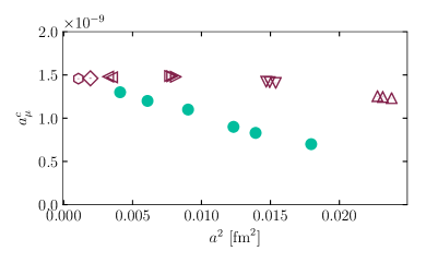
Figure 30: Comparison of the discretisation effects in $a_{\mu}^{c}$ in our results from Table 15 (red open symbols) and those from the BMW collaboration in Borsanyi et al. (2018) (filled blue circles) that use a less highly-improved staggered quark action. The filled blue circles only give estimates of the position of the BMW data points and do not indicate the statistical uncertainties which are much smaller than the size of the points.

Our new result for the pure QCD case (Eq. (40)) is compared to earlier lattice QCD results with realistic sea quark content in Fig. 29. Our new result (the top point on the plot) is much more accurate than the earlier results. With respect to the first calculation of $a_{\mu}^{c}$ that also used HISQ quarks Chakraborty et al. (2015) we have greatly reduced the previous dominant sources of uncertainty from $Z_{V}$ and the determination of the lattice spacing.

With respect to results using other formalisms, we give one figure to demonstrate the control of discretisation effects that is possible with the HISQ formalism. Figure 30 compares the approach to the continuum limit of our results (from Table 15) with results from BMWc Borsanyi et al. (2018), for which the continuum extrapolated result is shown in Fig. 29. The points plotted from Borsanyi et al. (2018) are estimates of the positions read from Figure S4, and do not include any indication of statistical uncertainties. The BMWc stout staggered quark action has $\mathcal{O}(a^{2})$ discretisation errors at tree-level since it uses an unimproved derivative in its version of the Dirac equation. Figure 30 shows that the price to be paid for not improving the discretisation is a very large discretisation effect. This is particularly evident when working with heavier quarks such as charm, since it means that the dominant $(\Lambda a)^{2}$ effects have $\Lambda\approx$ 1 GeV, as here. This means, for example, that the BMWc points at finest lattice spacing ($\sim$0.06 fm) are about as far (20% away) from the continuum limit as our points at our coarsest lattice spacing ($\sim$0.15 fm). Our results at $a\sim$ 0.06 fm are within 1% of the continuum limit, allowing us to achieve a sub-1% uncertainty in the final value.

We find that the impact of quenched QED on the result for $a_{\mu}^{c}$ is +0.214(19)% (Eq. 40). This is a shift in $a_{\mu}^{c}$ in the presence of the dominant QED effect of

$$\delta a_{\mu}^{c}=+0.0313(28)\times 10^{-10}.$$ (41)

We can compare this to the result obtained by ETMC in Giusti et al. (2019) following work on the QED effect on the renormalisation of quark bilinears in Di Carlo et al. (2019). The ETMC value is $+0.0182(36)\times 10^{-10}$, 2.8$\sigma$ smaller than ours.

The two calculations of the quenched QED effect are different. Ours is a direct calculation of the quenched QED effect, retuning the valence quark mass through determination of a meson mass in the usual way. The ETMC calculation is perturbative in quenched QED and fixes the valence quark masses so that they agree in the $\overline{\mathrm{MS}}$ scheme at 2 GeV in QCD+QED and pure QCD. It is likely that it is this difference in scheme for definining how QCD and QCD+QED are compared that is responsible for the tension between the two values. Our results in Section IV show that the quark mass in the $\overline{\mathrm{MS}}$ scheme is lower in QCD+QED than in QCD (at scales above $\overline{m}_{c}$) when the quark mass is tuned so that $M_{J/\psi}$ agrees with experiment in the two cases. This leads us to expect a larger result for the impact of quenched QED on $a_{\mu}^{c}$ with our tuning. Once full lattice QCD+QED calculations are underway tuning of the quark masses will be done through matching of meson masses to experiment.

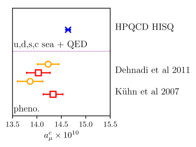
Figure 31: Comparison of our lattice QCD+QED result (blue cross) for the connected $c$ quark HVP contribution to $a_{\mu}$, $a_{\mu}^{c}$, with results determined from experimental information. The red open squares, denoted ‘pheno.’, use the charmonium moments from $R_{e^{+}e^{-}}$ given in Kuhn et al. (2007); Dehnadi et al. (2013) to determine $a_{\mu}^{c}$. The orange open circles give the alternative maximal (upper) and minimal (lower) inclusive cross-section datasets from Dehnadi et al. (2013).

Figure 31 includes a comparison of our result for $a_{\mu}^{c}$, now in QCD+QED, with values obtained using the moments determined from $J/\psi$ and $\psi^{\prime}$ properties and the inclusive cross-section for $e^{+}e^{-}\rightarrow{\mathrm{hadrons}}$, removing contributions from quarks other than $c$. The results for these moments from Kuhn et al. (2007); Dehnadi et al. (2013) were discussed and compared to our results in Section VI.2. In Fig. 31 we have converted the moments into a result for $a_{\mu}^{c}$ for comparison. As with the moments, we see a $2.5\sigma$ tension with the Dehnadi et al. (2013) result using the standard selection of datasets ($a_{\mu}^{c}=14.03(24)\times 10^{-10}$), and a larger tension with the minimal selection of datasets. There is agreement within 2$\sigma$ for the maximal selection of datasets from Dehnadi et al. (2013) and with Kuhn et al. (2007). Our result may then provide a pointer to the selection of $R_{e^{+}e^{-}}$ datasets for the phenomenological determination and/or indicate an issue with the perturbation theory used to subtract the $u/d/s$ contribution to obtain $R_{c}(s)$.

More recent determinations of the complete HVP contribution to $a_{\mu}$ using results from $R_{e^{+}e^{-}}$ are given in Keshavarzi et al. (2018); Davier et al. (2020). Although the $c$ component is not separated out, the contribution from the $J/\psi$ resonance is given as $6.26(19)\times 10^{-10}$ by Keshavarzi et al. (2018) and $6.20(11)\times 10^{-10}$ by Davier et al. (2020). We can also readily determine the contribution to $a_{\mu}^{c}$ from the $J/\psi$ resonance alone since in that case Chakraborty et al. (2016)

$$G_{n}=n!\frac{f_{J/\psi}^{2}}{M_{J/\psi}^{n}}\,.$$ (42)

Using our value for $f_{J/\psi}$ from Eq. (29) and the experimental value for $M_{J/\psi}$ Tanabashi et al. (2018) gives

$$a_{\mu}^{c}(J/\psi)=6.345(53)\times 10^{-10}.$$ (43)

This is in good agreement with the results determined above from the experimental $J/\psi$ parameters, but more accurate, reflecting the fact that our result for $\Gamma_{e^{+}e^{-}}$ in Fig. 24 agrees with experiment but has smaller uncertainty.

The $J/\psi$ contribution provides almost half of $a_{\mu}^{c}$ - we conclude that it is the rest of the contribution, from the inclusive cross-section above the resonance region, that causes the tension between our results for $a_{\mu}^{c}$ and that from $R_{e^{+}e^{-}}$ for some selections of experimental datasets. The tension then amounts to 7(3)% of this non-resonant cross-section.

VII Conclusions

We have performed the first $n_{f}=2+1+1$ lattice QCD computations of the properties of ground-state charmonium mesons. These have been done using the HISQ action to calculate quark-line connected two-point correlation functions on gluon field configurations that include $u/d$ quark masses going down to the physical point. The small discretisation effects in the HISQ action and high statistics achievable have given us good control over both the continuum and chiral extrapolations and has enabled us to obtain smaller uncertainties than previous lattice QCD computations of these properties (including previous calculations by HPQCD). At the same time we have improved the tuning of the bare $c$ quark mass to update the value of $\overline{m}_{c}$. From the same correlators that we use for the masses and decay constants we have also derived an improved result for the $c$ quark HVP contribution to the anomalous magnetic moment of the muon.

The precision possible for $c$ quark correlators with the HISQ action makes it possible to determine the impact of the $c$ quark’s electric charge. We do this directly and nonperturbatively in quenched QED by multiplying an appropriate U(1) field into our gluon field configurations. We tune the bare $c$ quark mass so that the $J/\psi$ mass agrees with experiment in both QCD+QED and QCD and we calculate mass and vector renormalisation constants in the RI-SMOM scheme in both cases, performing a full analysis as a function of $\mu$ to determine the $c$ quark mass in the $\overline{\mathrm{MS}}$ scheme.

Here we collect our final QCD+QED results (from Eqs. (10), (17), (29), (30), (40)) before discussing each in turn:

$$M_{J/\psi}-M_{\eta_{c}} =0.1203(11)\ \mathrm{GeV}$$

$$\overline{m}_{c}(3\ \mathrm{GeV}) =0.9841(51)\ \mathrm{GeV}$$

$$f_{J/\psi} =0.4104(17)\ \mathrm{GeV}$$

$$f_{\eta_{c}} =0.3981(10)\ \mathrm{GeV}$$

$$a_{\mu}^{c} =14.638(47)\times 10^{-10}.$$ (44)

Error budgets are given in Tables 5, 7, 11 and 16 respectively. Our error budgets do not include an error for missing QED effects for sea quarks or from having $m_{u}=m_{d}$ in the sea. We expect the former to dominate (see Sections II.3 and II.4) and estimate this at 10% of the size of the valence quark QED effects. This is then a negligible error in every case.

The precision of our result for the charmonium hyperfine splitting allows us to resolve, for the first time, the sign and magnitude of the anticipated difference between the lattice and experimental results arising from the fact that we do not include quark-line disconnected correlation functions. We take this difference to be the effect of the $\eta_{c}$ decay to two gluons which is prohibited in the lattice calculation, and conclude that $\Delta M_{\eta_{c}}^{\mathrm{annihln}}=+7.3(1.2)$ MeV.

The effect of QED on the hyperfine splitting is fairly substantial (1.4%) and the largest effect that we observe here. This has 3 components that all act in the same direction: a direct effect of 0.7%, 0.1% from retuning the $c$ quark mass and 0.6% from $J/\psi$ annihilation to a photon that we add by hand.

Our updated value of the charm quark mass (in the $\overline{\mathrm{MS}}$ scheme at a scale of 3 GeV) includes the effect of QED on the bare $c$ quark mass, tuned so that $M_{J/\psi}$ matches experiment, and on the mass renormalisation constant $Z_{m}$ determined on the lattice using the intermediate RI-SMOM scheme. The addition of results at a finer lattice spacing has improved the uncertainty slightly over HPQCD’s earlier result Lytle et al. (2018).

The impact of QED on $\overline{m}_{c}$ is small since QED effects tend to cancel between the retuning needed and changes in $Z_{m}$. At a scale of 3 GeV we see a -0.18(2)% effect, falling towards zero at a scale of $\overline{m}_{c}$.

Our result for the the $J/\psi$ decay constant is the most precise to date and acts as a subpercent test of QCD. The gain in precision from the 2012 HPQCD calculation of Donald et al. (2012) is a result of the use of a more accurate renormalisation of the vector current Hatton et al. (2019) as well as gluon field configurations with a wider range of sea $u/d$ quark masses and lattice spacing values. We can use our result for $f_{J/\psi}$ to determine a value for the width for $J/\psi$ decay to a lepton-antilepton pair (repeating Eq. (32)):

$$\Gamma(J/\psi\rightarrow e^{+}e^{-})=5.637(47)(13)\,\mathrm{keV}.$$ (45)

This is more accurate than the current average of experimental results Tanabashi et al. (2018).

The impact of quenched QED on $f_{J/\psi}$ is +0.2%, since the retuning of the $c$ quark mass offsets some of the direct effect. The effect on $f_{\eta_{c}}$ is almost the same so that the ratio of $f_{J/\psi}$ to $f_{\eta_{c}}$ remains the same. This ratio is determined here to be 1.0289(19), so that it is definitely greater than 1; this was not completely clear from earlier calculations.

Our results for the time-moments of the charmonium vector current-current correlators also provide a new level of accuracy for these quantities, improving by a factor of 10 over the first such calculations in Donald et al. (2012). Our results are given in Table 13. We see some tension for the lowest (4th) moment with phenomenological results derived from $R(e^{+}e^{-}\rightarrow\mathrm{hadrons})$ in Dehnadi et al. (2013) when particular selections of experimental datasets are made.

We use the time-moments to derive the connected $c$ quark HVP contribution to the anomalous magnetic moment of the muon, $a_{\mu}^{c}$. Although this is not a large part of the total HVP contribution and so improving its uncertainty has little impact on the full HVP contribution, nevertheless it is a piece that can be calculated very accurately in lattice QCD and provides a test case for comparison of lattice calculations and a comparison with phenomenology.

Our result for $a_{\mu}^{c}$ improves the accuracy by a factor of 3 over earlier lattice QCD values Chakraborty et al. (2015); Giusti et al. (2017); Borsanyi et al. (2018). Comparison of our result for $a_{\mu}^{c}$ to that determined from phenomenology can be divided into contributions from narrow resonances and from the continuum $e^{+}e^{-}\rightarrow c\overline{c}$. The contribution from the $J/\psi$ agrees well between our result and phenomenology, with our result being more accurate (see Section VI.4). This reflects the situation described above for $f_{J/\psi}$ and $\Gamma_{\ell\ell}$. The total $a_{\mu}^{c}$ derived from the time-moments determined from experimental data on $R(e^{+}e^{-}\rightarrow\mathrm{hadrons})$ when the component from a $c\overline{c}$ loop is separated out shows some tension with our results, depending on which experimental datasets are used above the resonance region. Our central value is higher, tending to reduce by a small amount the discrepancy in $a_{\mu}$ between existing experiment and the Standard Model. We should stress, however, that more complete determinations of $a_{\mu}$, for example in Keshavarzi et al. (2018); Davier et al. (2020), do not separate out $a_{\mu}^{c}$ and so we cannot make a direct comparison to them.

We also determine the impact of quenched QED on $a_{\mu}^{c}$ in a scheme in which the $c$ quark mass is tuned from $M_{J/\psi}$ in both QCD+QED and pure QCD. We find (repeating Eq. (41))

$$\delta a_{\mu}^{c}=+0.0313(28)\times 10^{-10}.$$ (46)

This is a 0.2% effect and dominated by the impact of retuning the $c$ quark mass.

Our result for $a_{\mu}^{c}$ has an accuracy of 0.3%. Sub-0.5% uncertainty is the aim for lattice QCD calculations of the full HVP contribution to $a_{\mu}$. We have shown that this is possible, for a small piece of the HVP, at least.

Acknowledgements

We are grateful to the MILC collaboration for the use of their configurations. We are also grateful for the use of MILC’s QCD code. We have modified it to generate quenched U(1) gauge fields and incorporate those into the quark propagator calculation as described here. We thank P. Knecht for contributions at the start of the project, C. McNeile for the calculation of $w_{0}/a$ and A. Keshavarzi, D. Miller, D. Nomura, D. Smaranda and T. Teubner for useful discussions. Computing was done on the Darwin supercomputer at the University of Cambridge High Performance Computing Service as part of the DiRAC facility, jointly funded by the Science and Technology Facilities Council, the Large Facilities Capital Fund of BIS and the Universities of Cambridge and Glasgow. We are grateful to the Darwin support staff for assistance. Funding for this work came from the Science and Technology Facilities Council and the National Science Foundation.

Appendix A $Z_{V}$ and $Z_{m}$ determination on the finest lattices

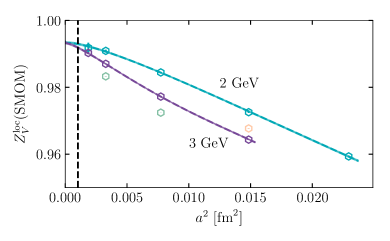
Figure 32: Results for the local vector current renormalisation factor in the RI-SMOM scheme compared to the fit form given in Eq. 47. All of the data points shown are included in the fit but only the 2 and 3 GeV fit lines are drawn. The data points not on the fit lines correspond to $\mu=$ 2.5 GeV (light orange) and 4 GeV (light green). The dashed line shows the value of $a$ on the exafine lattices that allows us to determine a $Z_{V}$ value there.

We can use the results of Hatton et al. (2019) to check the consistency of the $Z_{V}$ value on set 14 that we present here and to obtain a value on set 15. We do this by fitting the RI-SMOM results for the local vector current in Table III of Hatton et al. (2019) to the expected functional form. This form is based on a power series in $\alpha_{s}$ evaluated in the $\overline{\mathrm{MS}}$ scheme at a scale of $1/a$, which is the perturbative lattice-to-$\overline{\text{MS}}$ renormalisation factor, remembering that the SMOM to $\overline{\text{MS}}$ renormalisation factor is exactly 1 in this case. In addition we must allow for possible discretisation effects that depend on $a\mu$. The form we use is:

$$Z_{V}^{\mathrm{loc}}(\mathrm{SMOM})(a,\mu)=1+\sum_{i,j=1}^{i=4,j=3}\left[c_{i}+d_{ij}\left(\frac{a\mu}{\pi}\right)^{2j}\right]\alpha_{s}^{i}.$$ (47)

This is very similar to the approach adopted in Appendix B of Chakraborty et al. (2017b) using results for $Z_{V}$ from the determination of form factors between two identical mesons at rest. As there, we fix the $\alpha_{s}$ coefficient to its known perturbative value of -0.1164(3).

Fig. 32 shows the $Z_{V}$ data from Hatton et al. (2019) as hexagons, coloured according to their $\mu$ value. The fit lines for 2 and 3 GeV are also shown. The fit has a $\chi^{2}/\mathrm{dof}$ of 0.93. We note that the results from set 14 are included in this fit. The results from set 14, however, also agree with the fit result when they are not included in the fit. As discussed in Section IV $\mu$ was slightly mistuned on set 14; the true values are 2.04 and 2.98 GeV rather than 2 and 3 GeV. At this small lattice spacing the variation in $Z_{V}$ with $\mu$ (which is a discretisation effect) is small enough that this small mistuning can be neglected.

Note that the underlying perturbation theory of Eq. (47) should agree with that obtained from the fit in Chakraborty et al. (2017b) and it does. The discretisation effects are different in the two cases, of course. For RI-SMOM there is a momentum scale $\mu$ which we take as 2 GeV (although it can be taken as much smaller for $Z_{V}$ Hatton et al. (2019)) and this sets the size of discretisation effects as is clear from Figure 32.

Using the fit of Eq. (47) we may also extract $Z_{V}$ values at finer lattice spacings where it may not be practical for us to perform direct calculations due to the computational cost of Landau gauge fixing. This includes the exafine lattices of set 15 in Table 1 with a lattice spacing adjusted for sea-mass mistuning of 0.032 fm. The value of $Z_{V}$ from the fit for these lattices is 0.99296(21) at $\mu$ = 2 GeV and 0.99186(18) at 3 GeV.

Table 17: Values of $Z_{m}^{\mathrm{SMOM}}$ obtained in the RI-SMOM scheme on set 14 in pure QCD. Results are given at two values of $\mu$, listed in lattice units in column 1. They correspond approximately to 2 GeV and 3 GeV. The correlation between the two numbers is 0.122.

$a\mu$	$Z_{m}^{\mathrm{SMOM}}$
0.4466	1.2925(39)
0.6525	1.1785(11)

Results for the mass renormalisation factor from the lattice to the RI-SMOM scheme, $Z_{m}^{\mathrm{SMOM}}(\mu)$, determined on ultrafine set 14 are given in Table 17 at $\mu=$ 2 GeV and 3 GeV. These are calculated in the same way as that discussed in Lytle et al. (2018).

References

- Tanabashi et al. (2018) M. Tanabashi et al. (Particle Data Group), Phys. Rev. D98, 030001 (2018).
- Grange et al. (2015) J. Grange et al. (Muon g-2), (2015), arXiv:1501.06858 [physics.ins-det] .
- Bennett et al. (2004) G. W. Bennett et al. (Muon g-2), Phys. Rev. Lett. 92, 161802 (2004), arXiv:hep-ex/0401008 [hep-ex] .
- Boyle et al. (2017) P. Boyle, V. Gülpers, J. Harrison, A. Jüttner, C. Lehner, A. Portelli, and C. T. Sachrajda, JHEP 09, 153 (2017), arXiv:1706.05293 [hep-lat] .
- Giusti et al. (2019) D. Giusti, V. Lubicz, G. Martinelli, F. Sanfilippo, and S. Simula, Phys. Rev. D99, 114502 (2019), arXiv:1901.10462 [hep-lat] .
- Borsanyi et al. (2020) S. Borsanyi et al., (2020), arXiv:2002.12347 [hep-lat] .
- Cheung et al. (2016) G. K. Cheung, C. O’Hara, G. Moir, M. Peardon, S. M. Ryan, C. E. Thomas, and D. Tims (Hadron Spectrum), JHEP 12, 089 (2016), arXiv:1610.01073 [hep-lat] .
- Follana et al. (2007) E. Follana, Q. Mason, C. Davies, K. Hornbostel, G. P. Lepage, J. Shigemitsu, H. Trottier, and K. Wong (HPQCD, UKQCD), Phys. Rev. D75, 054502 (2007), arXiv:hep-lat/0610092 [hep-lat] .
- Bazavov et al. (2013) A. Bazavov et al. (MILC), Phys. Rev. D87, 054505 (2013), arXiv:1212.4768 [hep-lat] .
- Bazavov et al. (2018a) A. Bazavov et al., Phys. Rev. D98, 074512 (2018a), arXiv:1712.09262 [hep-lat] .
- Bernard and Toussaint (2018) C. Bernard and D. Toussaint (MILC), Phys. Rev. D 97, 074502 (2018), arXiv:1707.05430 [hep-lat] .
- Hart et al. (2009) A. Hart, G. M. von Hippel, and R. R. Horgan (HPQCD), Phys. Rev. D79, 074008 (2009), arXiv:0812.0503 [hep-lat] .
- Borsanyi et al. (2012) S. Borsanyi, S. Durr, Z. Fodor, C. Hoelbling, S. D. Katz, et al., JHEP 1209, 010 (2012), arXiv:1203.4469 [hep-lat] .
- Dowdall et al. (2013) R. Dowdall, C. Davies, G. Lepage, and C. McNeile (HPQCD), Phys.Rev. D88, 074504 (2013), arXiv:1303.1670 [hep-lat] .
- Monahan et al. (2013) C. Monahan, J. Shigemitsu, and R. Horgan, Phys. Rev. D87, 034017 (2013), arXiv:1211.6966 [hep-lat] .
- Hatton et al. (2019) D. Hatton, C. T. H. Davies, G. P. Lepage, and A. T. Lytle (HPQCD), Phys. Rev. D100, 114513 (2019), arXiv:1909.00756 [hep-lat] .
- Lepage et al. (2002) G. P. Lepage, B. Clark, C. T. H. Davies, K. Hornbostel, P. B. Mackenzie, C. Morningstar, and H. Trottier, Lattice field theory. Proceedings, 19th International Symposium, Lattice 2001, Berlin, Germany, August 19-24, 2001, Nucl. Phys. Proc. Suppl. 106, 12 (2002), arXiv:hep-lat/0110175 [hep-lat] .
- Dowdall et al. (2019) R. J. Dowdall, C. T. H. Davies, R. R. Horgan, G. P. Lepage, C. J. Monahan, J. Shigemitsu, and M. Wingate, Phys. Rev. D100, 094508 (2019), arXiv:1907.01025 [hep-lat] .
- Hayakawa and Uno (2008) M. Hayakawa and S. Uno, Prog. Theor. Phys. 120, 413 (2008), arXiv:0804.2044 [hep-ph] .
- Weisz (1983) P. Weisz, Nucl. Phys. B 212, 1 (1983).
- Hart et al. (2004) A. Hart, R. Horgan, and L. Storoni, Phys. Rev. D 70, 034501 (2004), arXiv:hep-lat/0402033 .
- Duncan et al. (1996) A. Duncan, E. Eichten, and H. Thacker, Phys. Rev. Lett. 76, 3894 (1996), arXiv:hep-lat/9602005 .
- de Divitiis et al. (2013) G. de Divitiis, R. Frezzotti, V. Lubicz, G. Martinelli, R. Petronzio, G. Rossi, F. Sanfilippo, S. Simula, and N. Tantalo (RM123), Phys. Rev. D 87, 114505 (2013), arXiv:1303.4896 [hep-lat] .
- Rosner et al. (2018) J. Rosner, S. Stone, and R. Van de Water (Particle Data Group review), in Phys. Rev. D98, 030001 (2018).
- Di Carlo et al. (2019) M. Di Carlo, D. Giusti, V. Lubicz, G. Martinelli, C. T. Sachrajda, F. Sanfilippo, S. Simula, and N. Tantalo, Phys. Rev. D100, 034514 (2019), arXiv:1904.08731 [hep-lat] .
- Amoros et al. (2001) G. Amoros, J. Bijnens, and P. Talavera, Nucl. Phys. B602, 87 (2001), arXiv:hep-ph/0101127 [hep-ph] .
- Chakraborty et al. (2015) B. Chakraborty, C. T. H. Davies, B. Galloway, P. Knecht, J. Koponen, G. C. Donald, R. J. Dowdall, G. P. Lepage, and C. McNeile, Phys. Rev. D91, 054508 (2015), arXiv:1408.4169 [hep-lat] .
- Basak et al. (2019) S. Basak et al. (MILC), Phys. Rev. D 99, 034503 (2019), arXiv:1807.05556 [hep-lat] .
- Davoudi and Savage (2014) Z. Davoudi and M. J. Savage, Phys. Rev. D90, 054503 (2014), arXiv:1402.6741 [hep-lat] .
- Gray et al. (2005) A. Gray, I. Allison, C. T. H. Davies, E. Dalgic, G. P. Lepage, J. Shigemitsu, and M. Wingate, Phys. Rev. D72, 094507 (2005), arXiv:hep-lat/0507013 [hep-lat] .
- Bouchard et al. (2014) C. M. Bouchard, G. P. Lepage, C. Monahan, H. Na, and J. Shigemitsu, Phys. Rev. D90, 054506 (2014), arXiv:1406.2279 [hep-lat] .
- Donald et al. (2012) G. C. Donald, C. T. H. Davies, R. J. Dowdall, E. Follana, K. Hornbostel, J. Koponen, G. P. Lepage, and C. McNeile, Phys. Rev. D86, 094501 (2012), arXiv:1208.2855 [hep-lat] .
- Xu et al. (2018) Q. N. Xu et al. (Belle), Phys. Rev. D98, 072001 (2018), arXiv:1805.03044 [hep-ex] .
- Aaij et al. (2015) R. Aaij et al. (LHCb), Eur. Phys. J. C75, 311 (2015), arXiv:1409.3612 [hep-ex] .
- Aaij et al. (2017a) R. Aaij et al. (LHCb), Phys. Lett. B769, 305 (2017a), arXiv:1607.06446 [hep-ex] .
- Aaij et al. (2017b) R. Aaij et al. (LHCb), Eur. Phys. J. C77, 609 (2017b), arXiv:1706.07013 [hep-ex] .
- Anashin et al. (2014) V. V. Anashin et al., Phys. Lett. B738, 391 (2014), arXiv:1406.7644 [hep-ex] .
- Lees et al. (2014) J. P. Lees et al. (BaBar), Phys. Rev. D89, 112004 (2014), arXiv:1403.7051 [hep-ex] .
- Ablikim et al. (2012a) M. Ablikim et al. (BESIII), Phys. Rev. Lett. 108, 222002 (2012a), arXiv:1111.0398 [hep-ex] .
- Ablikim et al. (2012b) M. Ablikim et al. (BESIII), Phys. Rev. D86, 092009 (2012b), arXiv:1209.4963 [hep-ex] .
- DeTar et al. (2019) C. DeTar, A. S. Kronfeld, S.-h. Lee, D. Mohler, and J. N. Simone (Fermilab Lattice, MILC), Phys. Rev. D99, 034509 (2019), arXiv:1810.09983 [hep-lat] .
- Briceno et al. (2012) R. A. Briceno, H.-W. Lin, and D. R. Bolton, Phys. Rev. D86, 094504 (2012), arXiv:1207.3536 [hep-lat] .
- Yang et al. (2015) Y.-B. Yang et al., Phys. Rev. D92, 034517 (2015), arXiv:1410.3343 [hep-lat] .
- Anashin et al. (2015) V. V. Anashin et al., Phys. Lett. B749, 50 (2015).
- Bodwin et al. (1995) G. T. Bodwin, E. Braaten, and G. P. Lepage, Phys. Rev. D51, 1125 (1995), [Erratum: Phys. Rev.D55,5853(1997)], arXiv:hep-ph/9407339 [hep-ph] .
- Levkova and DeTar (2011) L. Levkova and C. DeTar, Phys. Rev. D83, 074504 (2011), arXiv:1012.1837 [hep-lat] .
- Lytle et al. (2018) A. T. Lytle, C. T. H. Davies, D. Hatton, G. P. Lepage, and C. Sturm (HPQCD), Phys. Rev. D98, 014513 (2018), arXiv:1805.06225 [hep-lat] .
- Sturm et al. (2009) C. Sturm, Y. Aoki, N. H. Christ, T. Izubuchi, C. T. C. Sachrajda, and A. Soni, Phys. Rev. D80, 014501 (2009), arXiv:0901.2599 [hep-ph] .
- Kniehl and Veretin (2020) B. A. Kniehl and O. L. Veretin, (2020), arXiv:2002.10894 [hep-ph] .
- Bednyakov and Pikelner (2020) A. Bednyakov and A. Pikelner, (2020), arXiv:2002.12758 [hep-ph] .
- Bednyakov et al. (2017) A. Bednyakov, B. Kniehl, A. Pikelner, and O. Veretin, Nucl.Phys.B 916, 463 (2017), arXiv:1612.00660 [hep-ph] .
- Bazavov et al. (2018b) A. Bazavov et al. (Fermilab Lattice, MILC, TUMQCD), Phys. Rev. D98, 054517 (2018b), arXiv:1802.04248 [hep-lat] .
- Carrasco et al. (2014) N. Carrasco et al. (ETM), Nucl. Phys. B887, 19 (2014), arXiv:1403.4504 [hep-lat] .
- Keshavarzi et al. (2018) A. Keshavarzi, D. Nomura, and T. Teubner, Phys. Rev. D 97, 114025 (2018), arXiv:1802.02995 [hep-ph] .
- Anashin et al. (2018) V. V. Anashin et al. (KEDR), JHEP 05, 119 (2018), arXiv:1801.01958 [hep-ex] .
- Ablikim et al. (2016) M. Ablikim et al. (BESIII), Phys. Lett. B761, 98 (2016), arXiv:1604.01924 [hep-ex] .
- Anashin et al. (2012) V. V. Anashin et al., Phys. Lett. B711, 280 (2012), arXiv:1109.4215 [hep-ex] .
- Alexander et al. (1989) J. P. Alexander, G. Bonvicini, P. S. Drell, R. Frey, and V. Luth, Nucl. Phys. B320, 45 (1989).
- Fadin et al. (1994) V. S. Fadin, V. A. Khoze, and A. D. Martin, Phys. Lett. B320, 141 (1994), arXiv:hep-ph/9309234 [hep-ph] .
- Anashin et al. (2010) V. V. Anashin et al., Proceedings, 6th International Workshop on e+e- Collisions from Phi to Psi (PHIPSI09): Beijing, China, October 13-16, 2009, Chin. Phys. C34, 836 (2010), arXiv:1110.0328 [hep-ex] .
- Keshavarzi et al. (2020) A. Keshavarzi, D. Nomura, and T. Teubner, private communication (2020).
- Colquhoun et al. (2015) B. Colquhoun, C. T. H. Davies, R. J. Dowdall, J. Kettle, J. Koponen, G. P. Lepage, and A. T. Lytle (HPQCD), Phys. Rev. D91, 114509 (2015), arXiv:1503.05762 [hep-lat] .
- Davies et al. (2010) C. T. H. Davies, C. McNeile, E. Follana, G. P. Lepage, H. Na, and J. Shigemitsu, Phys. Rev. D82, 114504 (2010), arXiv:1008.4018 [hep-lat] .
- Kuhn et al. (2007) J. H. Kuhn, M. Steinhauser, and C. Sturm, Nucl. Phys. B778, 192 (2007), arXiv:hep-ph/0702103 [HEP-PH] .
- Bečirević et al. (2014) D. Bečirević, G. Duplančić, B. Klajn, B. Melić, and F. Sanfilippo, Nucl. Phys. B883, 306 (2014), arXiv:1312.2858 [hep-ph] .
- Bailas et al. (2018) G. Bailas, B. Blossier, and V. Morénas, Eur. Phys. J. C78, 1018 (2018), arXiv:1803.09673 [hep-lat] .
- Chakraborty et al. (2014) B. Chakraborty, C. T. H. Davies, G. C. Donald, R. J. Dowdall, J. Koponen, G. P. Lepage, and T. Teubner (HPQCD), Phys. Rev. D89, 114501 (2014), arXiv:1403.1778 [hep-lat] .
- Allison et al. (2008) I. Allison et al. (HPQCD), Phys. Rev. D78, 054513 (2008), arXiv:0805.2999 [hep-lat] .
- Blum (2003) T. Blum, Phys. Rev. Lett. 91, 052001 (2003), arXiv:hep-lat/0212018 [hep-lat] .
- Dehnadi et al. (2013) B. Dehnadi, A. H. Hoang, V. Mateu, and S. M. Zebarjad, JHEP 09, 103 (2013), arXiv:1102.2264 [hep-ph] .
- Nakayama et al. (2016) K. Nakayama, B. Fahy, and S. Hashimoto, Phys. Rev. D94, 054507 (2016), arXiv:1606.01002 [hep-lat] .
- Chakraborty et al. (2017a) B. Chakraborty, C. T. H. Davies, P. G. de Oliviera, J. Koponen, G. P. Lepage, and R. S. Van de Water, Phys. Rev. D96, 034516 (2017a), arXiv:1601.03071 [hep-lat] .
- Burger et al. (2014) F. Burger, X. Feng, G. Hotzel, K. Jansen, M. Petschlies, and D. B. Renner (ETM), JHEP 02, 099 (2014), arXiv:1308.4327 [hep-lat] .
- Giusti et al. (2017) D. Giusti, V. Lubicz, G. Martinelli, F. Sanfilippo, and S. Simula, JHEP 10, 157 (2017), arXiv:1707.03019 [hep-lat] .
- Borsanyi et al. (2018) S. Borsanyi et al. (Budapest-Marseille-Wuppertal), Phys. Rev. Lett. 121, 022002 (2018), arXiv:1711.04980 [hep-lat] .
- Davier et al. (2020) M. Davier, A. Hoecker, B. Malaescu, and Z. Zhang, Eur. Phys. J. C 80, 241 (2020), arXiv:1908.00921 [hep-ph] .
- Chakraborty et al. (2016) B. Chakraborty, C. Davies, J. Koponen, G. Lepage, M. Peardon, and S. Ryan, Phys. Rev. D 93, 074509 (2016), arXiv:1512.03270 [hep-lat] .
- Chakraborty et al. (2017b) B. Chakraborty, C. T. H. Davies, G. C. Donald, J. Koponen, and G. P. Lepage (HPQCD), Phys. Rev. D96, 074502 (2017b), arXiv:1703.05552 [hep-lat] .