Finite Step Performance of First-order Methods Using Interpolation Conditions Without Function Evaluations

Abstract

We present a procedure to numerically compute finite step worst case performance guarantees on a given algorithm for the unconstrained optimization of strongly convex functions with Lipschitz continuous gradients. The solution method provided serves as an alternative approach to that derived by Taylor, Hendrickx, and Glineur in [Math. Prog. 161 (1-2), 2017]. The difference lies in the fact that our solution uses conditions for the interpolation of a set of points and gradient evaluations by the gradient of a function in the class of interest, whereas their solution uses conditions for the interpolation of a set of points, gradient evaluations, and function evaluations by a function in the class of interest. The motivation for this alternative solution is that, in many cases, neither the algorithm nor the performance metric of interest rely upon function evaluations. The primary development is a procedure to avoid suffering from the factorial growth in the number of these conditions with the size of the set to be interpolated when solving for the worst case performance.

I Introduction

In recent years, there has been efforts to understand the worst case performance of first-order black box optimization algorithms on specific problem classes. The problem class that has received the most attention by far is the unconstrained optimization of smooth, convex functions. There have been two primary versions of worst case performance bounds defined for this problem class. These are the finite step ($N$-step) and asymptotic performance bounds.

We present a means of numerically solving for the worst case $N$-step performance of a given first-order method on strongly convex functions with Lipschitz continuous gradients. The unconstrained optimization is $\min_{x\in\mathbb{R}^{d}}f(x)$, where $f$ is in a specified set of functions $\mathcal{F}$. The approach is derived by considering conditions for a set of points $\{(y_{i},u_{i})\}_{i=1}^{N}$ to be interpolated by the gradient of a function in the class of interest, i.e. $u_{i}=\nabla f(y_{i})$ for some $f\in\mathcal{F}$. Furthermore, we present a method to construct functions in the problem class on which the algorithm achieves the worst case performance. The contributions rely largely upon a few key technical results, many of which are readily available in the literature and are discussed in Section III. The primary development is then presented in Section IV. The development may be summarized as follows: we write conic combinations of the interpolation conditions using doubly hyperdominant matrices, thereby reducing the dimension of the optimization problem solved to yield the numerical performance bounds. This also enables a procedure to reduce the number of constraints in the optimization problem solved to generate worst case trajectories.

The solution presented is not the first means of solving the worst case $N$-step performance problem. The problem is formally posed in [1], and upper bounds on the worst case performance are found. In [2], an exact solution to the problem is found by developing necessary and sufficient conditions for a set of points $\{(y_{i},u_{i},f_{i})\}_{i=1}^{N}$ to be interpolable by a function and its gradient, i.e $u_{i}=\nabla f(y_{i})$ and $f_{i}=f(y_{i})$ for some $f\in\mathcal{F}$. As the bound is exact, it is possible to construct a function in the class of interest attaining the worst case performance.

Interpolation conditions which do not involve the function evaluations $\{f_{i}\}_{i=1}^{N}$ are presented in [3]. The drawback is that the number of conditions scales factorially with the size of the set to be interpolated. This fact deterred the use of such conditions for solving the worst case performance problem. The method proposed in our paper avoids this factorial growth in the worst-case $N$-step performance analysis. Specifically, we demonstrate that the performance can be computed by solving optimization problems with $O(N^{2})$ constraints. This approach also yields example functions that achieve the computed performance. It should be noted that the class of functions considered in [2] is slightly broader than that considered here, as it allows for the analysis of problem classes which include functions that are not strongly convex. Additionally, the performance measures used in [2] are more general than what is considered here. In particular, our performance measures may not include function evaluations, while theirs can.

The solution approach outlined in this paper for finding worst case trajectories draws inspiration from [4], which provides a way of constructing worst case trajectories of a linear system constrained to satisfy a set of integral quadratic constraints. While their problem is focused on asymptotic analysis, we present a related result for finite horizon analysis of linear systems satisfying a set of integral quadratic constraints. The construction is simpler than in the asymptotic case, and it arises almost immediately from our proof of the lossless S-Procedure.

The primary motivation for solving the worst case performance problem using interpolation conditions that do not involve function evaluations is that many first order algorithms rely solely upon gradient evaluations. Therefore, introducing function evaluations as an implicit constraints is an unnecessary step for the analysis of such algorithms. Furthermore, the approach proposed in our paper can be used to assess the performance of feedback systems with nonlinear elements, e.g. saturation. This avoids the introduction of implicit constraints upon the “function” evaluations which have no physical meaning in these analyses.

Numerical comparisons between the $N$-step performance bound solved via the approach outlined in this paper and an asymptotic performance bound are presented in Section V. It is interesting to note that on the example considered, the decay rate of the $N$-step performance bound with $N$ almost perfectly matches the asymptotic convergence rate.

Notation: The Euclidean norm of $y\in\mathbb{R}^{d}$ is denoted $\|y\|$. The Kronecker product of two matrices $A$ and $B$ is represented as $A\otimes B$. A symmetric, positive semidefinite matrix $A=A^{\top}$ is denoted by $A\succeq 0$. Similarly, $A\succeq B$ denotes that $A-B$ is positive semidefinite. The set of symmetric $n\times n$ matrices will be called $\mathbb{S}^{n}$.

II Problem Statement

II-A Terminology

A function $f:\mathbb{R}^{d}\mapsto\mathbb{R}$ is convex if the following inequality holds for all $y_{1},y_{2}\in\mathbb{R}^{d}$ and $\theta\in[0,1]$:

$$f(\theta y_{1}+(1-\theta)y_{2})\leq\theta f(y_{1})+(1-\theta)f(y_{2}).$$ (1)

Next, let $m>0$ be given and define $g:\mathbb{R}^{d}\mapsto\mathbb{R}$ by $g(y):=f(y)-\frac{m}{2}\|y\|^{2}$. The function $f$ is $m$-strongly convex if $g$ is convex. Finally, $f$ has $L$-Lipschitz gradients for some $L<\infty$ if the function is differentiable and the following inequality holds for all $y_{1},y_{2}\in\mathbb{R}^{d}$:

$$\|\nabla f(y_{2})-\nabla f(y_{1})\|\leq L\|y_{2}-y_{1}\|.$$ (2)

This inequality implies that the gradient of $f$ is continuous. The class of $m$-strongly convex functions with $L$-Lipshitz gradients is denoted by $S_{m,L}$. We will also use the notation $S_{m,L}$ when $m=0$ and/or $L=\infty$. The case $m=0$ corresponds to functions that are convex but not necessarily strongly convex. The case $L=\infty$ includes functions that need not be differentiable. In this case, the subdifferential of $f$ at point $y$ is denoted by $\partial f(y)$.

II-B Performance Bounds

Consider the unconstrained minimization of the function $f:\mathbb{R}^{d}\mapsto\mathbb{R}$:

$$\min_{y\in\mathbb{R}^{d}}f(y)$$ (3)

The function $f$ is assumed to be in $S_{m,L}$ with $0<m<L<\infty$. This ensures that Equation 3 has a unique minimizer $y_{*}$.

First-order algorithms use gradient evaluations to generate a sequence of iterates $\{y_{0},y_{1},\ldots\}$ that converge to the minimizer $y_{*}$. We focus on algorithms that can be expressed as a linear, time-varying (LTV) system in feedback with the gradient. Let $A_{k}\in\mathbb{R}^{n\times n}$, $B_{k}\in\mathbb{R}^{n\times 1}$ and $C_{k}\in\mathbb{R}^{1\times n}$ be given for each $k$ and define the algorithm as:

$$\begin{split}x_{k+1}&=(A_{k}\otimes I_{d})\,x_{k}+(B_{k}\otimes I_{d})\,u_{k}\\ y_{k}&=(C_{k}\otimes I_{d})\,x_{k}\\ u_{k}&=\nabla f(y_{k}).\end{split}$$ (4)

Here $u_{k}\in\mathbb{R}^{d}$, $y_{k}\in\mathbb{R}^{d}$, and $x_{k}\in\mathbb{R}^{nd}$ are the input, output, and state at iterate $k$. This includes linear, time-invariant (LTI) algorithms as a special case, i.e. the case where $(A,B,C)$ do not depend on the iteration $k$.

This formulation in Equation 4 follows the work in [5] and covers a large class of algorithms. For example, $(A_{k},B_{k},C_{k}):=(1,-\alpha_{k},1)$ corresponds to gradient descent with varying stepsize: $y_{k+1}=y_{k}-\alpha_{k}\nabla f(y_{k})$. As a second example, define the first-order algorithm with the state $x_{k}:=\begin{bmatrix}y_{k}^{T}&y_{k-1}^{T}\end{bmatrix}^{T}$ and the following matrices:

$$A:=\begin{bmatrix}(1+\beta)&-\beta\\ 1&0\end{bmatrix},\,\,B:=\begin{bmatrix}-\alpha\\ 0\end{bmatrix},\,\,C:=\begin{bmatrix}1&0\end{bmatrix}.$$ (5)

This corresponds to the heavy-ball algorithm with constant parameters:

$$y_{k+1}=y_{k}-\alpha\nabla f(y_{k})+\beta(y_{k}-y_{k-1})$$ (6)

Other algorithms can be modeled as in Equation 4 including Nesterov’s accelerated method [6] and the triple momentum method [7].

We assume the algorithm has an optimal state $x_{*}$ corresponding to the minimizer $y_{*}$. Thus for each $f\in S_{m,L}$ there is a state $x_{*}$ such that $x_{0}=x_{*}$ yields the iterates $x_{k}=x_{*}$ and $y_{k}=y_{*}$ for $k=0,1,\ldots$. Note that the minimizer $y_{*}$ satisfies $\nabla f(y_{*})=0$. Thus the state $x_{*}$ must satisfy

$$x_{*}=(A_{k}\otimes I_{d})x_{*}\mbox{ and }y_{*}=(C_{k}\otimes I_{d})x_{*}.$$ (7)

The optimal states for gradient descent and heavy-ball are $x_{*}=y_{*}$ and $x_{*}:=\begin{bmatrix}(y_{*})^{T}&(y_{*})^{T}\end{bmatrix}^{T}$, respectively.

We consider finite-step worst-case performance over all functions $f\in S_{m,L}$. The performance bound of interest is formally defined next.

Definition 1.

Consider a time-varying algorithm defined by $\{A_{k}\}_{k=0}^{N-1}$, $\{B_{k}\}_{k=0}^{N-1}$, and $\{C_{k}\}_{k=0}^{N}$. The worst-case, $N$-step performance bound on $S_{m,L}$ is the smallest value of $b$ such that for any $f\in S_{m,L}$:

$$\|y_{N}-y_{*}\|\leq b\|x_{0}-x_{*}\|.$$

This definition bounds the convergence of the iterate $y_{k}$ to the minimizer $y_{*}$. More general performance measures are considered in [2], including convergence of the function values $f(y_{k})$ to the minimal value $f(y_{*})$.

In the remainder of the paper we assume that $y_{*}=0$ and $x_{*}=0$. This assumption simplifies the notation and is without loss of generality by a coordinate shift. Specifically, assume $f\in S_{m,L}$ is minimized at $y_{*}\neq 0$ and the algorithm has an optimal state $x_{*}\neq 0$. Redefine the algorithm state and output to be $\tilde{x}_{k}:=x_{k}-x_{*}$ and $\tilde{y}_{k}:=y_{k}-y_{*}$. Define the shifted function $\tilde{f}\in S_{m,L}$ by $\tilde{f}(\tilde{y}):=f(\tilde{y}+y_{*})$. The shifted function $\tilde{f}$ has $\tilde{y}=0$ as its minimizer. Moreover, the finite-step performance bound is unchanged by this coordinate shift.

III Technical Results

Prior to presenting the solution to the worst case performance problem, we derive a series of technical results. Many of these results are readily available in the literature, and references are provided for more detailed proofs.

III-A Interpolation Conditions

Consider the set $\{(y_{i},u_{i})\}_{i\in\mathcal{I}}\subset\mathbb{R}^{d}\times\mathbb{R}^{d}$ with $\mathcal{I}:=\{0,\ldots,R\}$. This subsection presents conditions to interpolate this finite set of data by the gradient of a function in $S_{m,L}$.

Definition 2.

The set $\{(y_{i},u_{i})\}_{i\in\mathcal{I}}$ is $S_{m,L}$ interpolable for $0\leq m<L\leq\infty$ if there exists $f\in S_{m,L}$ such that:

• ($L<\infty$): $\nabla f(y_{i})=u_{i}$ for all $i\in\mathcal{I}$.

• ($L=\infty$): $u_{i}\in\partial f(y_{i})$ for all $i\in\mathcal{I}$.

Lemma 4, stated below, provides a necessary and sufficient condition for $S_{m,L}$ interpolation with $0<m<L<\infty$. This result is available as Lemma 3.25 of [3]. The proof is a variation of the proof of Theorem 4 in [2] which provides interpolation conditions involving both gradient and function evaluations. Definition 2 also allows $m=0$ and/or $L=\infty$ because these cases are needed for intermediate technical results. Cyclic monotonicity, defined next, plays a key role in the various interpolation conditions.

Definition 3.

The set $\{(y_{i},u_{i})\}_{i\in\mathcal{I}}$ is cyclically monotone if the following inequality holds for any cycle of indices $\{i_{0},i_{1},\ldots,i_{J}=i_{0}\}$:

$$\sum_{j=0}^{J-1}u_{i_{j}}^{\top}(y_{i_{j+1}}-y_{i_{j}})\leq 0$$ (8)

We first state a condition from [8] for a finite set of data to be $S_{0,\infty}$ interpolable.

Lemma 1.

The set $\{(y_{i},u_{i})\}_{i\in\mathcal{I}}$ is $S_{0,\infty}$ interpolable if and only if it is cyclically monotone.

Proof.

Assume the set is $S_{0,\infty}$ interpolable, i.e. there exists $f\in S_{0,\infty}$ such that $u_{i}\in\partial f(y_{i})$ for all $i\in\mathcal{I}$ and hence:

$$f(y)\geq f(y_{i})+u_{i}^{\top}(y-y_{i})\,\,\,\forall y\in\mathbb{R}^{d}$$ (9)

Apply this inequality to any cycle $\{i_{0},i_{1},\ldots,i_{J}=i_{0}\}$:

$$f(y_{i_{j+1}})\geq f(y_{i_{j}})+u_{i_{j}}^{\top}(y_{i_{j+1}}-y_{i_{j}})$$ (10)

Sum these inequalities from $j=0$ to $j=J$ to demonstrate that Equation 8 holds. This is valid for any cycle and hence the finite set of data is cyclically monotone. This direction of the proof is formally stated as Theorem 24.8 of [9].

Conversely, assume the set is cyclically monotone. Then by Theorem 3.4 in [8] there is a function $f\in S_{0,\infty}$ that interpolates the data. ∎

If the data is cyclically monotone then there are many choices for an interpolating function in $S_{0,\infty}$. Theorem 3.4 and Proposition 3.5 in [8] provides an explicit construction for an interpolating function of the form:

$$f(y)=\max_{i\in\mathcal{I}}\left[\lambda_{i}+u_{i}^{\top}(y-y_{i})\right]$$ (11)

The constants $\{\lambda_{i}\}_{i\in\mathcal{I}}$ are computed from a linear program and satisfy $f(y_{i})=\lambda_{i}$. This construction is a pointwise maximum of affine functions. The construction simplifies further if the data is one-dimensional ($d=1$). Details for the case with $d=1$ are provided in Section 8 of [8].

Next, two additional supporting lemmas are presented before stating the main result.

Lemma 2.

The set $\{(y_{i},u_{i})\}_{i\in\mathcal{I}}$ is $S_{m,L}$ interpolable if and only if the set $\{(y_{i},u_{i}-my_{i})\}_{i\in\mathcal{I}}$ is $S_{0,L-m}$ interpolable.

Proof.

Suppose $f\in S_{m,L}$ interpolates $\{(y_{i},u_{i})\}_{i\in\mathcal{I}}$. Define the function $g$ by $g(y):=f(y)-\frac{m}{2}\|y\|^{2}$. Then $g$ is in $S_{0,L-m}$ and it interpolates $\{(y_{i},u_{i}-my_{i})\}_{i\in\mathcal{I}}$. The converse follows similarly. ∎

Lemma 3.

The set $\{(y_{i},u_{i})\}_{i\in\mathcal{I}}$ is $S_{0,L}$ interpolable if and only if the set $\{(u_{i},y_{i})\}_{i\in\mathcal{I}}$ is $S_{1/L,\infty}$ interpolable.

Proof.

Suppose $f\in S_{m,L}$ interpolates $\{(y_{i},u_{i})\}_{i\in\mathcal{I}}$. Define the conjugate of $f$ by $f^{*}(u):=\sup_{y}u^{\top}y-f(y)$. It follows from Proposition 12.60 of [10] that $f^{*}$ interpolates $\{(u_{i},y_{i})\}_{i\in\mathcal{I}}$ and is in $S_{1/L,\infty}$. Proposition 12.60 also demonstrates the converse. In particular, if a function in $S_{1/L,\infty}$ interpolates $\{(u_{i},y_{i})\}_{i\in\mathcal{I}}$ then its conjugate is in $S_{0,L}$ and interpolates $\{(y_{i},u_{i})\}_{i\in\mathcal{I}}$. ∎

Finally, we state the main interpolation result for $S_{m,L}$ with $0<m<L<\infty$.

Lemma 4.

(Lemma 3.25 in [3]) The set $\{(y_{i},u_{i})\}_{i\in\mathcal{I}}$ is $S_{m,L}$ interpolable with $0<m<L<\infty$ if and only if $\{(Ly_{i}-u_{i},u_{i}-my_{i})\}_{i\in\mathcal{I}}$ is cyclically monotone.

Proof.

The five statements below are equivalent. Lemma 2 implies $1\leftrightarrow 2$ and $3\leftrightarrow 4$. Lemma 3 implies $2\leftrightarrow 3$ and $4\leftrightarrow 5$.

1. $\{(y_{i},u_{i})\}_{i\in\mathcal{I}}$ is $S_{m,L}$ interpolable.

2. $\{(y_{i},u_{i}-my_{i})\}_{i\in\mathcal{I}}$ is $S_{0,L-m}$ interpolable.

3. $\{(u_{i}-my_{i},y_{i})\}_{i\in\mathcal{I}}$ is $S_{1/(L-m),\infty}$ interpolable.

4. $\{(u_{i}-my_{i},\,\frac{1}{L-m}(Ly_{i}-u_{i})\}_{i\in\mathcal{I}}$ is $S_{0,\infty}$ interpolable.

5. $\{(\frac{1}{L-m}(Ly_{i}-u_{i}),\,u_{i}-my_{i}\}_{i\in\mathcal{I}}$ is $S_{0,\infty}$ interpolable.

Finally, Lemma 1 implies condition 5) is equivalent to cyclic monotonicity of $\{(Ly_{i}-u_{i},u_{i}-my_{i})\}_{i\in\mathcal{I}}$. This step requires factoring the constant $\frac{1}{L-m}>0$ from each term in the cyclic mononotinicity constraint. ∎

If the set $\{(Ly_{i}-u_{i},u_{i}-my_{i})\}_{i\in\mathcal{I}}$ is cyclically monotone then an interpolating function in $S_{m,L}$ can be constructed as follows. First, use Lemma 1 to construct a function $f_{4}\in S_{0,\infty}$ that interpolates the data in Statement 4. This can be done with a pointwise maximum of affine functions as in Equation 11. Next, interpolate the data in Statement 3 with $f_{3}\in S_{1/(L-m),\infty}$ defined by $f_{3}(y):=f_{4}(y)+\frac{1}{2(L-m)}\|y\|^{2}$. Interpolate the data in Statement 2 by taking the conjugate: $f_{2}=f_{3}^{*}\in S_{0,L-m}$. Note that evaluating $f_{2}(y)$ involves solving the maximization in the definition of the conjugate. Hence the function $f_{2}$ does not, in general, have an explicit expression. Finally, interpolate the original data with $f_{1}\in S_{m,L}$ defined by $f_{1}(y):=f_{2}(y)+\frac{m}{2}\|y\|^{2}$.

III-B S-Procedure

Let $M_{0},M_{1},\ldots,M_{L}\in\mathbb{S}^{\ell}$ be given and define quadratic functions $\sigma_{i}:\mathbb{R}^{\ell d}\mapsto\mathbb{R}$ for $i=0,\ldots,L$ by:

$$\sigma_{i}(\eta):=\eta^{\top}(M_{i}\otimes I_{d})\eta$$ (12)

The matrices $M_{i}$ are not necessarily sign definite. This section reviews a technical result to answer the following question: Let $\eta\neq 0$ be given. Does $\sigma_{i}(\eta)\geq 0$ for $i=1,\ldots,L$ imply that $\sigma_{0}(\eta)\geq 0$? The next lemma provides an exact linear matrix inequality condition to answer this question. This is known as the (lossless) S-procedure, discussed in Section 2.6.3 of [11]. The formulation below is essentially from [12] (see Theorem 7 and Appendices A/B).

In order to ensure that the optimization problems considered throughout the remainder of this section attain their optimal solutions, we require the following assumption:

Assumption 1.

There exists an $\eta\in\{\eta|\sigma_{i}(\eta)\geq 0,i=1,\ldots,L\}$ such that when $\eta\in\mathbb{R}^{\ell d}$ is partitioned as:

$$\eta:=\begin{bmatrix}\eta_{1}\\ \vdots\\ \eta_{\ell}\end{bmatrix}\mbox{ where each }\eta_{i}\in\mathbb{R}^{d}$$

and the blocks are stacked into a matrix $B:=\begin{bmatrix}\eta_{1},\ldots,\eta_{\ell}\end{bmatrix}\in\mathbb{R}^{d\times\ell}$, $B$ has rank $\geq\ell$.

We demonstrate in Section IV that this assumption holds for the constraints applied to solve the $N$-step performance problem.

Lemma 5.

Consider the following two statements involving the quadratic functions in Equation 12

1. If $\eta\neq 0$ and $\sigma_{i}(\eta)\geq 0$ for $i=1,\ldots,L$ then $\sigma_{0}(\eta)\geq 0$.

2. There exists non-negative scalars $\{\lambda_{1},\ldots,\lambda_{L}\}$ such that $M_{0}-\sum_{i=1}^{L}\lambda_{i}M_{i}\succeq 0$.

Statement 2) implies 1). Moreover, if $d\geq\ell$ and Assumption 1 holds, then Statement 1) implies 2).

Proof.

(2$\rightarrow$ 1) Note that 2) implies:

$$(M_{0}\otimes I_{d})-\sum_{i=1}^{L}\lambda_{i}(M_{i}\otimes I_{d})\succeq 0$$

Multiply on the right and left by any $\eta$ and $\eta^{T}$ to obtain:

$$\sigma_{0}(\eta)\geq\sum_{i=1}^{L}\lambda_{i}\sigma_{i}(\eta)$$

Statement 1 follows from this inequality and using $\lambda_{i}\geq 0$.

(1$\rightarrow$ 2) Assume Statement 1 holds and $d\geq\ell$. Consider the following optimization:

$$p_{*}= \min_{\eta\in\mathbb{R}^{\ell d}}\sigma_{0}(\eta)$$

$$\mbox{subject to: }\|\eta\|=1$$

$$\hskip 44.80704pt\sigma_{i}(\eta)\geq 0\mbox{ for }i=1,\ldots,L$$

Note that Statement 1 implies that $\sigma_{0}(\eta)\geq 0$ for any feasible $\eta$ for this optimization and hence $p_{*}\geq 0$.

Next, partition, $\eta\in\mathbb{R}^{\ell d}$ as follows:

$$\eta:=\begin{bmatrix}\eta_{1}\\ \vdots\\ \eta_{\ell}\end{bmatrix}\mbox{ where each }\eta_{i}\in\mathbb{R}^{d}$$

Stack the partitioned blocks of $\eta$ into a matrix $B:=\begin{bmatrix}\eta_{1},\ldots,\eta_{\ell}\end{bmatrix}\in\mathbb{R}^{d\times\ell}$. It can be shown, using the Kronecker product structure, that $\sigma_{i}(\eta)=\mathrm{Tr}(M_{i}B^{\top}B)$ for $i=0,\ldots,L$. As a consequence, the minimization can be equivalently written in terms of $G:=B^{\top}B\in\mathbb{S}^{\ell}$.

$$\begin{split}p_{*}=&\min_{G\in\mathbb{S}^{\ell}}\mathrm{Tr}(M_{0}G)\\ &\mbox{subject to: }\mathrm{Tr}(G)=1,\,G\succeq 0\\ &\hskip 44.80704pt\mathrm{Tr}(M_{i}G)\geq 0\mbox{ for }i=1,\ldots,L\\ &\hskip 44.80704pt\mbox{Rank}(G)\leq d\end{split}$$

The rank constraint is satisfied due to the additional assumption that $d\geq\ell$. Hence the rank constraint can be removed to yield a convex, semidefinite program (SDP):

$$\begin{split}p_{*}=&\min_{G\in\mathbb{S}^{\ell}}\mathrm{Tr}(M_{0}G)\\ &\mbox{subject to: }\mathrm{Tr}(G)=1,\,G\succeq 0\\ &\hskip 44.80704pt\mathrm{Tr}(M_{i}G)\geq 0\mbox{ for }i=1,\ldots,L\\ \end{split}$$ (13)

The dual of this SDP is:

$$\begin{split}d_{*}=&\max_{\nu,\lambda_{i}\in\mathbb{R}}\nu\\ &\mbox{subject to: }\lambda_{i}\geq 0\mbox{ for }i=1,\ldots,L\\ &\hskip 44.80704ptM_{0}-\sum_{i=1}^{L}\lambda_{i}M_{i}\succeq\nu I_{n}\end{split}$$ (14)

The dual has a strictly feasible point, e.g. choose any $\lambda_{i}>0$ and $\nu$ sufficiently negative. As a consequence, strong duality holds and the primal attains its optimal solution, see Section 5.9.1 of [13]. By Assumption 1, the primal has a feasible point $G$ for which $G\succ 0$. Then by Proposition 6.3.2 in [14], the dual problem attains its optimal solution. As noted above, Statement 1 implies $p_{*}\geq 0$ and, by strong duality, $d_{*}\geq 0$. It follows that there exists $\lambda_{i}\geq 0$ and $\nu\geq 0$ such that $M_{0}-\sum_{i=1}^{L}\lambda_{i}M_{i}\succeq\nu I_{n}$. Thus Statement 2 holds. ∎

III-C Construction of a Worst-Case Counterexample

Suppose Statement 2 in Lemma 5 is false and $d\geq\ell$. The proof of Lemma 5 can be used to construct an $\eta\in\mathbb{R}^{\ell d}$ that demonstrates the falsity of Statement 1. Specifically, if Statement 2 is false then $M_{0}-\sum_{i=1}^{L}\lambda_{i}M_{i}\nsucceq 0$ for all nonnegative scalars $\{\lambda_{1},\ldots,\lambda_{L}\}$. As a result the optimal value of the dual problem (14) satisfies $d_{*}<0$. Moreover, strong duality implies $p_{*}=d_{*}<0$. Let $G_{*}\succeq 0$ denote a corresponding optimal solution to the primal problem (13). Perform a rank factorization $G_{*}=B_{*}^{\top}B_{*}$ where $B_{*}\in\mathbb{R}^{d\times\ell}$. (This step may require rows of zeros to be appended to $B_{*}$ to ensure it has row dimension $d$.) Denote the $i^{th}$ column of $B_{*}$ by $\eta_{i}$ and define $\eta_{*}:=\begin{bmatrix}\eta_{1}^{\top}&\eta_{2}^{\top}&\ldots&\eta_{\ell}^{\top}\end{bmatrix}^{\top}$. The primal feasibility of $G_{*}$ implies that $\|\eta_{*}\|=\mathrm{Tr}(G_{*})=1$ and $\sigma_{i}(\eta_{*})=\mathrm{Tr}(M_{i}G_{*})\geq 0$ for $i=1,\ldots,L$. Moreover, $\sigma_{0}(\eta_{*})=\mathrm{Tr}(M_{0}G_{*})=p_{*}<0$. Thus $\eta_{*}$ is a specific vector demonstrating that Statement 1 is false.

A key step in this construction is the numerical solution to the primal problem (13). This is computationally costly if the number of constraints $L$ is large. In some instances, a primal optimal value $G_{*}$ can be obtained by first solving the dual, and then solving the primal with only a subset of constraints. In particular, let $(\nu_{*},\lambda_{*})$ be any optimal solution to the dual (14) and define $\mathcal{J}:=\{i\,:\,\lambda_{*,i}>0\}$. Define the following modified primal problem enforcing only the subset of constraints given by $\mathcal{J}$:

$$\begin{split}p_{*,\mathcal{J}}=&\min_{G\in\mathbb{S}^{\ell}}\mathrm{Tr}(M_{0}G)\\ &\mbox{subject to: }\mathrm{Tr}(G)=1,\,G\succeq 0\\ &\hskip 44.80704pt\mathrm{Tr}(M_{i}G)\geq 0\mbox{ for }i\in\mathcal{J}\end{split}$$ (15)

The associated dual of this modified primal problem is:

$$\begin{split}d_{*,\mathcal{J}}=&\max_{\nu,\lambda_{i}\in\mathbb{R}}\nu\\ &\mbox{subject to: }\lambda_{i}\geq 0\mbox{ for }i\in\mathcal{J}\\ &\hskip 44.80704ptM_{0}-\sum_{i\in\mathcal{J}}\lambda_{i}M_{i}\succeq\nu I_{n}\end{split}$$ (16)

This leads to the following result.

Lemma 6.

If the modified primal problem (15) has a unique solution, $G_{*,\mathcal{J}}$, then this is also a solution to the original primal problem (13).

Proof.

First note that the feasible set of the modified dual problem (16) is a subset of the feasible set for the original dual problem (14). Thus $d_{*}\geq d_{*,\mathcal{J}}$. Moreover, the optimal point $(v_{*},\lambda_{*})$ for (14) is also feasible for the modified dual problem (16). This point achieves the cost $d_{*}$ and hence is also optimal for (16), i.e. $d_{*,\mathcal{J}}=d_{*}$. Next recall that strong duality holds for the original problems, i.e. $p_{*}=d_{*}$, as noted in the proof of Lemma 5. Similarly, strong duality holds for the modified problems, i.e. $p_{*,\mathcal{J}}=d_{*,\mathcal{J}}$, because (16) also has a strictly feasible point. It follows from these results that the two primal problems achieve the same cost $p_{*}=p_{*,\mathcal{J}}$. Finally, the modified primal problem (15) only has a subset of the constraints enforced for the original primal problem (13). Thus any optimal solution $G_{*}$ to the original primal problem (13) is also optimal for the modified primal (15). In other words, the set of optimal points for the modified primal includes all optimal points for the original primal. By assumption, the modified primal problem has a unique optimal $G_{*,\mathcal{J}}$. Thus $G_{*,\mathcal{J}}$ is also optimal for the original primal problem. ∎

If the assumptions of Lemma 6 hold then a worst-case counterexample can be constructed as follows. First solve the original dual problem to find the active dual variables $\mathcal{J}:=\{i\,:\,\lambda_{*,i}>0\}$ for any optimal point. Next solve the modified primal problem (15) to obtain $G_{*,\mathcal{J}}$. If this solution is unique then $G_{*}=G_{*,\mathcal{J}}$. The remaining steps at the beginning of this section can be used to construct the counterexample $\eta_{*}$. The final technical result in this section is a condition that can be used to verify if the modified primal problem has a unique solution. This follows from the uniqueness and nondegeneracy results in [15].

Definition 4.

Let $(\nu,\lambda)$ be any feasible point for the modified dual problem in (16). Perform the eigenvalue decomposition

$$M_{0}-\sum_{i\in\mathcal{J}}\lambda_{i}M_{i}-\nu I=\begin{bmatrix}Q_{1}&Q_{2}\end{bmatrix}\begin{bmatrix}\Gamma&0\\ 0&0\end{bmatrix}\begin{bmatrix}Q_{1}^{\top}\\ Q_{2}^{\top}\end{bmatrix},$$ (17)

where $\Gamma\in\mathbb{R}^{s\times s}$ is a diagonal matrix containing the nonzero eigenvalues. The point $(\nu,\lambda)$ is non-degenerate if $\{I\}\cup\{Q_{2}^{\top}M_{i}Q_{2}\}_{i\in\mathcal{J}}$ spans $\mathbb{S}^{\ell-s}$.

Lemma 7.

Let $(\nu_{*},\lambda_{*})$ be an optimal solution to (16) with $\lambda_{*,i}>0$ for $i\in\mathcal{J}$. If this point is non-degenerate then (15) has a unique solution.

Proof.

Let $G_{*}$ and $(\nu_{*},\lambda_{*})$ denote optimal solutions to the modified primal/ dual problems (dropping the subscript $\mathcal{J}$ to simplify the notation). These must satisfy the following complementary slackness conditions, as discussed in Section 5.5.2 of [13]:

$$\lambda_{*,i}\mathrm{Tr}(M_{i}G_{*})=0\mbox{ for }i\in\mathcal{J}$$ (18)

$$Z_{*}G_{*}=0$$ (19)

where $Z_{*}=M_{0}-\sum_{i\in\mathcal{J}}\lambda_{*,i}M_{i}-\nu_{*}I$. Let $([Q_{1},Q_{2}],\Gamma)$ be an eigendecomposition of $Z_{*}$ as in Equation 17. By Lemma 1 in [15], $G_{*}$ and $Z_{*}$ share eigenvectors. Thus there exists a $U_{1}\in\mathbb{S}^{s}$ and $U_{2}\in\mathbb{S}^{\ell-s}$ such that

$$G_{*}=\begin{bmatrix}Q_{1}&Q_{2}\end{bmatrix}\begin{bmatrix}U_{1}&0\\ 0&U_{2}\end{bmatrix}\begin{bmatrix}Q_{1}^{\top}\\ Q_{2}^{\top}\end{bmatrix}$$

To achieve $Z_{*}G_{*}=0$, we must have $\Gamma U_{1}=0$. The eigenvalues in $\Gamma$ are assumed to be non-zero. It follows that $U_{1}=0$ and hence $G_{*}=Q_{2}U_{2}Q_{2}^{\top}$. Primal feasibilty of $G_{*}$ implies $1=\mathrm{Tr}(G_{*})=\mathrm{Tr}(U_{2})$. In addition, the complementary slackness conditions in Equation 18 combined with $\lambda_{i,*}>0$ imply that $0=\mathrm{Tr}(M_{i}G_{*})=\mathrm{Tr}(Q_{2}^{\top}M_{i}Q_{2}U_{2})$ for $i\in\mathcal{J}$. These conditions are summarized as

$$\mathrm{Tr}((Q_{2}^{\top}M_{i}Q_{2})U_{2})=0\mbox{ for }i\in\mathcal{J}$$

$$\mathrm{Tr}((I)U_{2})=1$$

The non-degeneracy assumptions impies that these conditions uniquely define $U_{2}$ and hence $G_{*}$. ∎

III-D Conic Combinations of Cyclic Monotonicity Constraints

The technical results in the previous subsections can be used to compute the worst case $N$-step performance bound. This will be described in detail in the next section. One issue is that the number of cyclic monontonicity constraints scales with $N!$. This subsection provides a final technical result to alleviate this computational growth. Specifically, it is shown that conic combinations of cyclic monotonicity conditions may be written using doubly hyperdominant matrices.

To see that this is so, first consider the set of data $\{(y_{i},u_{i})\}_{i=0}^{R-1}$. By Lemma 1, this data is $S_{0,\infty}$ interpolable if and only if it is cyclically monotone. It is useful to slightly reformulate of the cyclic monotonicity conditions. The set $\{(y_{i},u_{i})\}_{i=0}^{R-1}$ is cyclically monotone if and only if the following inequality holds for any permutation $\{i_{0},i_{1},\ldots,i_{R-1}\}$ of the indices $\{0,\ldots,R-1\}$:

$$\sum_{j=0}^{R-1}u_{j}^{\top}(y_{j}-y_{i_{j}})\geq 0$$ (20)

Define the stacked data $U_{0:R-1}:=\begin{bmatrix}u_{0}^{\top},\ldots,u_{R-1}^{\top}\end{bmatrix}$ and similarly for $Y_{0:R-1}$. The data is cyclically monotone if and only if the following constraints are satisfied for each $R\times R$ permutation matrix $\{P_{i}\}_{i=1}^{R!}$:

$$U_{0:R-1}^{\top}\,((I-P_{i})\otimes I_{d})\,Y_{0:R-1}\geq 0$$ (21)

Next define the following set:

$$\mathcal{M}_{R}:=\left\{\sum_{i=1}^{R!}\lambda_{i}(I-{P}_{i})\,:\,\lambda_{i}\geq 0\right\}.$$

Any conic combination of the cyclic monotonicity constraints has the following form for some $W\in\mathcal{M}_{R}$:

$$U_{0:R-1}^{\top}\,(W\otimes I_{d})\,Y_{0:R-1}\geq 0$$ (22)

Such conic combinations can be equivalently written with doubly hyperdominant matrices as defined next.

Definition 5.

A matrix is doubly hyperdominant if the off diagonal elements are nonpositive, and both the row sums and column sums are nonnegative. A matrix is doubly hyperdominant with zero excess if it is doubly hyperdominant, and both the row sums and column sums are zero.

Let $\mathcal{H}_{R}$ denote the set of $R\times R$ doubly hyperdominant matrices. The subset of doubly hyperdominant matrices with zero excess is denoted $\mathcal{H}_{R}^{0}$.

Lemma 8.

The set $\mathcal{H}_{R}^{0}$ is equal to the set $\mathcal{M}_{R}$.

Proof.

Take any $W\in\mathcal{M}_{R}$ so that, by definition, there exists nonnegative $\{\lambda_{i}\}_{i=1}^{R!}$ such that:

$$W=\sum_{i=1}^{R!}\lambda_{i}(I-{P}_{i})$$ (23)

Each term $\lambda_{i}(I-P_{i})$ has nonpositive off-diagonal entries and row/colums that sum to zero. Thus the sum in Equation 23 is doubly hyperdominant with zero excess, i.e. $\mathcal{M}_{R}\subseteq\mathcal{H}_{R}^{0}$.

Next take any $H\in\mathcal{H}_{R}^{0}$. It follows from Theorem 3.7 in [16] that $H\in\mathcal{M}_{R}$. In particular, let $r$ be any constant greater than the diagonal elements of $H$. Then $H=r[I-S]$ where $S:=\frac{1}{r}(rI-H)$ has all nonnegative entries with row/column sums equal to $1$. $S$ is a doubly stochastic matrix and hence it can be decomposed as a convex combination of permutation matrices. This is the Birkhoff/von-Neumann decomposition [17]. In other words, there exist permutation matrices $\{P_{i}\}_{i=1}^{k}$ and nonnegative $\{\alpha_{i}\}_{i=1}^{k}$ such that $\sum_{i=1}^{k}\alpha_{i}=1$ and $S=\sum_{i=1}^{k}\alpha_{i}P_{i}$. The Birkhoff algorithm [18] provides one specific decomposition. This decomposition can be performed with no more than $k\leq R^{2}-2R+1$ terms. Define the nonnegative scalars $\lambda_{i}:=r\alpha_{i}$ to obtain the decomposition $H=\sum_{i=1}^{k}\lambda_{i}(I-P_{i})$. Thus $H\in\mathcal{M}_{R}$. ∎

IV Performance Bound

IV-A Formulation

The technical results in the previous section are now used to compute the worst case N-step performance bound. Consider the unconstrained minimization of $f:\mathbb{R}^{d}\mapsto\mathbb{R}$ as in (3). As noted earlier, we assume without loss of generality that $y_{*}=0$ is the optimal point. Let $\{A_{k}\}_{k=0}^{N-1},\{B_{k}\}_{k=0}^{N-1}$, and $\{C_{k}\}_{k=0}^{N}$ define a time-varying algorithm of the form (4). Moreover, let $\{x_{k}\}_{k=0}^{N},\{u_{k}\}_{k=0}^{N-1}$, and $\{y_{k}\}_{k=0}^{N}$ be the sequence of iterates generated by this algorithm starting from the intial state $x_{0}$. The worst-case, $N$-step performance bound on $S_{m,L}$ is the smallest value of $b$ such that $\|y_{N}\|\leq b\|x_{0}\|$ holds for any $f\in S_{m,L}$.

Each iterate in the finite horizon sequences can be expressed as a linear combination of $x_{0}$ and $\{u_{k}\}_{k=0}^{N-1}$. Define the vector $\eta:=\begin{bmatrix}x_{0}^{\top}&U_{0:N-1}^{\top}\end{bmatrix}^{\top}\in\mathbb{R}^{n_{\eta}}$ with dimension $n_{\eta}:=(N+n)d$. Let $R_{0}$ and $R_{1}$ be matrices that define the following mapppings:

$$\begin{split}&x_{0}:=(R_{0}\otimes I_{d})\eta,\\ &y_{N}:=(R_{1}\otimes I_{d})\eta,\end{split}$$ (24)

For example $R_{0}:=\begin{bmatrix}I_{n}&0_{n\times N}\end{bmatrix}\in\mathbb{R}^{n\times(N+n)}$. The matrix $R_{1}$ can be constructed from the state matrices of the LTV algorithm.

The performance bound can be expressed in terms of the matrices defined in Equation 24. Define the quadratic function $\sigma_{0}:\mathbb{R}^{n_{\eta}}\times\mathbb{R}\rightarrow\mathbb{R}$ by $\sigma_{0}(\eta,b):=\eta^{\top}(M_{0}(b)\otimes I_{d})\eta$ where $M_{0}(b):=b^{2}R_{0}^{\top}R_{0}-R_{1}^{\top}R_{1}$. By the definitions in 24, $\sigma_{0}(\eta,b)=b^{2}\|x_{0}\|^{2}-\|y_{N}\|^{2}$. Hence the bound $\|y_{N}\|\leq b\|x_{0}\|$ is satisfied if and only if $\sigma_{0}(\eta,b)\geq 0$.

Similarly, quadratic functions can be defined to encode the cyclic monotonticity constraints. By Lemma 4, the data $\{u_{k}\}_{k=0}^{N-1}$ and $\{y_{k}\}_{k=0}^{N-1}$ is $S_{m,L}$ interpolable if and only if $\{(Ly_{i}-u_{i},u_{i}-my_{i})\}_{i=0}^{N-1}$ is cyclically monotone. As noted earlier, we consider, without loss of generality, the case where $y_{*}=0$ is the optimal point. This occurs when $\nabla f(0)=0$. Thus all functions under consideration have gradients that interpolate $(0,0)$. The cyclic monotonicity conditions, including the point $(0,0)$, are thus given by:

$$(LY_{0:N-1}-U_{0:N-1})^{\top}(Q_{i}\otimes I_{d})(U_{0:N-1}-mY_{0:N-1})\geq 0$$

$$\mbox{where }Q_{i}:=\left[\begin{smallmatrix}0\\ I\end{smallmatrix}\right]^{\top}\,(I-P_{i})\,\left[\begin{smallmatrix}0\\ I\end{smallmatrix}\right]$$

The additional blocks of zeros account for the point $(0,0)$. This inequality must hold for all $(N+1)\times(N+1)$ permutation matrices $P_{i}$. Let $R_{2L}$ and $R_{2m}$ be matrices that define the following mappings:

$$\begin{split}&LY_{0:N-1}-U_{0:N-1}:=(R_{2L}\otimes I_{d})\,\eta\\ &U_{0:N-1}-mY_{0:N-1}:=(R_{2m}\otimes I_{d})\,\eta\end{split}$$ (25)

Define the quadratic functions $\sigma_{i}:\mathbb{R}^{n_{\eta}}\rightarrow\mathbb{R}$ by $\sigma_{i}(\eta)=\eta^{\top}(M_{i}\otimes I_{d})\eta$ where

$$M_{i}:= \frac{1}{2}\begin{bmatrix}R_{2L}\\ R_{2m}\end{bmatrix}^{\top}\begin{bmatrix}0&Q_{i}\\ Q_{i}^{\top}&0\end{bmatrix}\begin{bmatrix}R_{2L}\\ R_{2m}\end{bmatrix}$$

$$\mbox{ for }i=1,\ldots,(N+1)!$$

The cyclic monotonicity conditions are thus equivalent to $\sigma_{i}(\eta)\geq 0$ for $i=1,\ldots,(N+1)!$.

A quadratic function of arbitrary dimension dimension can be constructed to verify that Assumption 1 holds for these conditions. The construction is based on an example due to Nesterov [19] and details can be found in Appendix B of [12].

IV-B Worst Case Performance

We now state the main result which supplies a means to calculate the $N$-step worst case performance bound.

Theorem 1.

The worst case $N$-step performance of the algorithm defined by $\{A_{k}\}_{k=0}^{N-1}$, $\{B_{k}\}_{k=0}^{N-1}$, $\{C_{k}\}_{k=0}^{N}$ on $S_{m,L}$ is given by the optimal value to

$$b_{*} :=\min_{H\in\mathcal{H}_{N},b\in\mathbb{R}}b$$ (26)

$$\mbox{subject to: }M_{0}(b)-\left[\begin{smallmatrix}R_{2L}\\ R_{2m}\end{smallmatrix}\right]^{\top}\left[\begin{smallmatrix}0&H\\ H^{\top}&0\end{smallmatrix}\right]\left[\begin{smallmatrix}R_{2L}\\ R_{2m}\end{smallmatrix}\right]\succeq 0.$$

Proof.

Recall that we may, without loss of generality, consider functions achieving their minimum at the origin. The worst-case $N$-step performance problem is to find the smallest $b$ such that $\|y_{N}\|\leq b\|x_{0}\|$ whenever $N$ steps of algorithm (4) are run on $f\in S_{m,L}$ from the intial state $x_{0}\in\mathbb{R}^{nd}$. Running (4) on functions $f\in S_{m,L}$ will generate sequences of iterates $\{(y_{i},u_{i})\}_{i=0}^{N-1}$ that are $S_{m,L}$ interpolable. It follows from Lemma 4 and the notation above that the iterates are $S_{m,L}$ interpolable if and only if $\sigma_{i}(\eta)\geq 0$ for $i=1,\ldots,(N+1)!$. Likewise, $\|y_{N}\|\leq b\|x_{0}\|$ is equivalent to $\sigma_{0}(\eta,b)\geq 0$.

Thus the $N$-step worst case performance is given by the solution to the following optimization:

$$\begin{split}&\min_{b\in\mathbb{R}}b\\ &\mbox{subject to: }\sigma_{0}(\eta,b)\geq 0\mbox{ for all }\eta\in\mathbb{R}^{n_{\eta}}\mbox{ satisfying}\\ &\hskip 44.80704pt\sigma_{i}(\eta)\geq 0\mbox{ for }i=1\ldots(N+1)!\end{split}$$

By Lemma 5, this is equivalent to

$$\begin{split}&\min_{b\in\mathbb{R},\lambda_{i}\in\mathbb{R}}b\\ &\mbox{subject to: }\lambda_{i}\geq 0\mbox{ for }i=1,\ldots,(N+1)!\\ &\hskip 44.80704ptM_{0}(b)-\sum_{i=1}^{(N+1)!}\lambda_{i}M_{i}\succeq 0\end{split}$$

The conic combinations of $M_{i}$ may be expressed in terms of the set $\mathcal{M}_{N}$ to express the above problem as

$$\begin{split}&\min_{b\in\mathbb{R},W\in\mathcal{M}_{N}}b\\ &\mbox{subject to:}\\ &M_{0}(b)-\left[\begin{smallmatrix}R_{2L}\\ R_{2m}\end{smallmatrix}\right]^{\top}\left[\begin{smallmatrix}0&\left[\begin{smallmatrix}0\\ I\end{smallmatrix}\right]^{\top}W\left[\begin{smallmatrix}0\\ I\end{smallmatrix}\right]\\ \left[\begin{smallmatrix}0\\ I\end{smallmatrix}\right]^{\top}W^{\top}\left[\begin{smallmatrix}0\\ I\end{smallmatrix}\right]&0\end{smallmatrix}\right]\left[\begin{smallmatrix}R_{2L}\\ R_{2m}\end{smallmatrix}\right]\succeq 0.\end{split}$$

Apply Lemma 8 to replace $W\in\mathcal{M}_{N}$ with $\hat{H}\in\mathcal{H}_{N}^{0}$. The term $\left[\begin{smallmatrix}0\\ I\end{smallmatrix}\right]^{\top}\hat{H}\left[\begin{smallmatrix}0\\ I\end{smallmatrix}\right]$ eliminates the first row and column of $H$. Let $H$ be the sub-matrix obtained by removing the first row and column of $\hat{H}$. Then $H$ is doubly hyperdominant but possibly with excess, i.e. $H\in\mathcal{H}_{N}$. This leads to the formulation in (26). ∎

Note that (26) is a semidefinite program (SDP) in the variables $b$ and $H\in\mathcal{H}_{N}$. The number of independent variables in the doubly hyperdominant matrix scales with $N^{2}$ even though the cyclic monotonicity conditions involve $N!$ constraints. This SDP can be efficiently solved (for moderate horizon lengths) using freely available software.

IV-C Worst Case Trajectory

The bound computed by Theorem 1 is exact. In particular, let $b^{*}$ be the optimal value found from Theorem 1. Select any $b\in(0,b^{*})$ and $d\geq N+n$. There is a function $f\in S_{m,L}$ achieving its minimum at $y_{*}=0$ and an initial state $x_{0}$ such that the final value of the algorithm has $\|y_{N}\|>b\|x_{0}\|$.

The procedure in Section III-C can be used to construct a feasible sequence of iterates iterpolable by such a function. In particular, if $b<b^{*}$ then $M_{0}-\sum_{i=1}^{L}\lambda_{i}M_{i}\nsucceq 0$ for all nonnegative scalars $\{\lambda_{1},\ldots,\lambda_{L}\}$. As a result, the construction at the beginning of Section III-C provides an $\eta\neq 0$ with $\sigma_{i}(\eta)\geq 0$ for $i=1,\ldots,(N+1)!$ and $\sigma_{0}(\eta)<0$. This vector can be mapped to a sequence $\{(y_{i},u_{i})\}_{i=0}^{N-1}$ which is interpolable by an $f\in S_{m,L}$ with optimal value at $y_{*}=0$. Furthermore, $\sigma_{0}(\eta)<0$ imples $\|y_{N}\|>b\|x_{0}\|$.

This procedure requires the solution to the optimization problem (13). As noted in Section III-C, the number of constraints grows factorially with $N$. The remainder of Section III-C provides a method that scales quadratically with $N$. First let $(\nu_{*},H_{*})$ be optimal for the following problem:

$$\begin{split}&\max_{\nu\in\mathbb{R},H\in\mathcal{H}_{N}}\nu\\ &\mbox{subject to: }M_{0}(b)-\left[\begin{smallmatrix}R_{2L}\\ R_{2m}\end{smallmatrix}\right]^{\top}\left[\begin{smallmatrix}0&H\\ H^{\top}&0\end{smallmatrix}\right]\left[\begin{smallmatrix}R_{2L}\\ R_{2m}\end{smallmatrix}\right]\succeq\nu I_{n}\end{split}$$ (27)

Append an additional row/and column to $H_{*}$ to obtain the corresponding matrix with zero excess, $\hat{H}_{*}$ such that: $H_{*}=\left[\begin{smallmatrix}0\\ I_{R}\end{smallmatrix}\right]^{\top}\hat{H}_{*}\left[\begin{smallmatrix}0\\ I_{R}\end{smallmatrix}\right]$. This may be done by setting the elements of the added row/column to the negation of the corresponding column/row sum respectively. Decompose $\hat{H}_{*}$ as described in the proof of Lemma 8, and denote the coefficients for the decomposition by $\lambda_{*}$. Then $(\nu_{*},\lambda_{*})$ solve (14). Furthermore, if we let $\mathcal{J}=\{i|\lambda_{*,i}>0\}$ and $(\nu_{*},\lambda_{*})$ is non-degenerate, then a solution to (15) is also a solution to (13). As $\mathcal{J}$ has at most $(N+1)^{2}-2(N+1)+1$ elements, the number of constraints in (13) scales quadratically with $N$.

V Numerical Results

Theorem 1 provides an approach to calculate the $N$-step worst case performance $b_{*}$ of an algorithm on $S_{m,L}$. As noted previously, the optimization problem (26) is a semidefinite program and can be efficiently solved for moderate horizons. Section IV-C provides a method to construct specific worst-case trajectories that are arbitrarily close to $b_{*}$. The code to compute the worst case performance as well as to find worst case trajectories will be available Github. The code was tested, in part, by verifying that the performance bounds attained match those found using the Performance Estimation Toolkit [20] which is based on the results in [2].

The method was used to compute the $N$-step performance bounds for the heavy-ball (Equations 5 and 6). The algorithm parameters were selected to optimize performance on quadratic functions:

$$\alpha:=\frac{4}{(\sqrt{L}+\sqrt{m})^{2}}\mbox{ and }\beta:=\left(\frac{\sqrt{L}-\sqrt{m}}{\sqrt{L}+\sqrt{m}}\right)^{2}$$

Figure 1 shows the $N$-step performance bounds for several values of $N$ (blue-x). The left plot is for $m=1,L=10$ and the right plot is for $m=1,L=30$. This algorithm is known to converge asymptotically to the optimal value if and only if the condition ratio satisfies $\frac{L}{m}<9+4\sqrt{5}$ [21]. The left subplot corresponds to a condition ratio below this boundary and the finite-step bounds decay, as expected. The right subplot corresponds to a condition ratio above this boundary and the finite-step bounds increase, as expected.

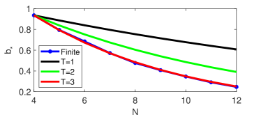
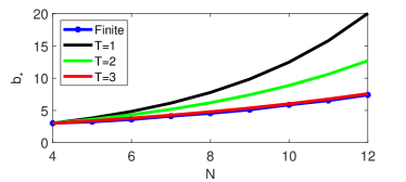
Figure 1: Finite Step and Asymptotic $S_{m,L}$ Performance Bounds on Heavy Ball Algorithm Optimized for Quadratics. Top plot is for $m=1$, $L=10$ and bottom plot is for $m=1$ and $L=30$.

It is interesting to compare the $N$-step performance bounds with estimates of the asymptotic convergence rate. One asymptotic result is briefly presented as it provides a baseline for comparison.

Theorem 2.

Consider an LTI algorithm defined by $(A,B,C)$ run on $f\in S_{m,L}$ achieving its minimum at the origin. For a positive integer $T$, define

$$\eta_{k} :=\begin{bmatrix}x_{k-T}\\ U_{(k-T):(k-1)}\end{bmatrix}$$ (28)

$$z_{k} :=\begin{bmatrix}LY_{(k-T):(k-1)}-U_{(k-T):(k-1)}\\ -mY_{(k-T):(k-1)}+U_{(k-T):(k-1)}\end{bmatrix}$$ (29)

Let $(\hat{A}\otimes I_{d},\hat{B}\otimes I_{d},\hat{C}\otimes I_{d},\hat{D}\otimes I_{d})$ define the state space system with input $u_{k}$, state $\eta_{k}$, and output $z_{k}$. Define the optimization:

$$\rho_{*} :=\min_{\rho\in\mathbb{R},P\in\mathbb{S}^{T+n},H\in\mathcal{H}_{T}}\rho$$

$$\mbox{subject to:}\hskip 7.22743ptP\succ 0$$

$$\hskip 44.80704pt\begin{bmatrix}\rho^{2}P&0\\ 0&0\end{bmatrix}-\begin{bmatrix}\hat{A}^{\top}\\ \hat{B}^{\top}\end{bmatrix}P\begin{bmatrix}\hat{A}^{\top}\\ \hat{B}^{\top}\end{bmatrix}^{\top}$$

$$\hskip 52.03448pt-\begin{bmatrix}\hat{C}^{\top}\\ \hat{D}^{\top}\end{bmatrix}\begin{bmatrix}0&H\\ H^{\top}&0\end{bmatrix}\begin{bmatrix}\hat{C}^{\top}\\ \hat{D}^{\top}\end{bmatrix}^{\top}\succeq 0$$

Then there exists a constant $c>0$ such that for all $k$, $\|y_{k}\|\leq c\rho_{*}^{k}\|\eta_{0}\|$.

Proof.

Similar asymptotic performance bounds and detailed proofs are found in [5] and [12]. A sketch is given here. Let $(\rho_{*},P_{*},H_{*})$ be optimal for the minimization in the theorem statement. Define $V(\eta):=\eta^{\top}P\eta$. As in the finite-step results, the interpolability conditions imply:

$$\begin{bmatrix}\eta_{k}\\ u_{k}\end{bmatrix}^{\top}\begin{bmatrix}\hat{C}^{\top}\\ \hat{D}^{\top}\end{bmatrix}\begin{bmatrix}0&H\\ H^{\top}&0\end{bmatrix}\begin{bmatrix}\hat{C}^{\top}\\ \hat{D}^{\top}\end{bmatrix}^{\top}\begin{bmatrix}\eta_{k}\\ u_{k}\end{bmatrix}\succeq 0$$

Thus the matrix inequality in the minimization implies that $V(\eta_{k+1})\leq\rho^{2}V(\eta_{k})$ for each $k$. Iterating this inequality yields $\|\eta_{k}\|\leq c\rho_{*}^{k}\|\eta_{0}\|$ by setting $c=\sqrt{\frac{\lambda_{max}(P)}{\lambda_{min}(P)}}$. Then $\|y_{k}\|\leq\|C\|c\rho_{*}^{k}\|\eta_{0}\|$, where $\|C\|$ is the induced two norm of $\|C\|$. ∎

It should be noted that unlike the finite horizon performance bound, the asymptotic bound is not guaranteed to be tight. In particular, $\rho_{*}$ only serves as an upper bound, in general, for the asymptotic convergence rate. As such, there are numerous variations of the bounding approach in Theorem 2 which supply different upper bounds on the asymptotic convergence, e.g. [5] and [12].

Figure 1 also shows the asymptotic rate $\rho_{*}$ for several different values of $T$. The constant $c$ for the asymptotic curves is chosen so that each curve aligns with the finite-step bound at $N=4$. This allows for easier comparison. One notable aspect of these plots is that the asymptotic rate with $T=3$ agrees, within numerical tolerances, to the finite horizon results. The finite horizon results are exact and hence this raises interesting conjectures regarding the exactness of the asymptotic bounds with $T$ sufficiently large. We also note that the results obtained using the optimization in Theorem 2 with $T=3$ are strictly tighter than the bounds provided in [5] or [12]. The examples on Github provide this comparison and a further comparison of various conditions to compute asymptotic rates will be explored in future work.

VI Conclusion

Our contribution is to provide a novel means of solving the finite step worst case performance problem. The solution relies upon necessary and sufficient conditions for a set of data including points and gradient evaluations to be interpolable by the gradient of a strongly convex function with Lipschitz continuous gradients. Despite factorial growth in the number of interpolation constraints with the size of the data set, we demonstrate that the numerical solutions to the performance bounding problem may be found from solutions to optimization problems whose constraints grow only quadratically with the time horizon.

The motivation for solving the problem in this manner is that a large class of algorithms do not rely upon function evaluations, so introducing them into the constraints is unnecessary.

It was also seen that the interpolation conditions derived can be extended to the case of asymptotic algorithm analysis by straightforward application of the framework from [5]. Using the asymptotic bound found by this procedure, we illustrate a connection between the finite step and asymptotic performance bounds in Section V. The numerical results suggest that the solution to the finite step performance bounding problem may provide insight into the problem of bounding the asymptotic convergence rate. Further exploration of the relationship between the problems is left as future work.

References

• [1] Y. Drori and M. Teboulle โ€œPerformance of first-order methods for smooth convex minimization: a novel approachโ€ In Mathematical Programming 145, 2014, pp. 451โ€“482
• [2] Adrien B. Taylor, Julien M. Hendrickx and Francois Glineur โ€œSmooth Strongly Convex Interpolation and Exact Worst-case Performance of First-order Methodsโ€ In Mathematical Programming 161, 2017, pp. 307โ€“345
• [3] Adrien Taylor โ€œConvex interpolation and pe rformance estimation of first-order methods for convex optimizationโ€, 2017
• [4] Bryan Van Scoy and Laurent Lessard โ€œIntegral Quadratic Constraints: Exact Convergence Rates and Worst-Case Trajectoriesโ€ In IEEE 58th Annual Conference on Decision and Control (CDC), 2019, pp. 7677โ€“7682
• [5] Laurent Lessard, Benjamin Recht and Andrew Packard โ€œAnalysis and design of optimization algorithms via integral quadratic constraintsโ€ In SIAM Journal on Optimization 26.1 SIAM, 2016, pp. 57โ€“95
• [6] Y. E. Nesterov โ€œA method for solving the convex programming problem with convergence rate O$(1/k^{2})$โ€ In Dokl. Akad. Nauk SSSR 269, 1983, pp. 543โ€“547
• [7] B. Van Scoy, R. A. Freeman and K. M. Lynch โ€œThe Fastest Known Globally Convergent First-Order Method for Minimizing Strongly Convex Functionsโ€ In IEEE Control Systems Letters 2.1, 2018, pp. 49โ€“54
• [8] D. Lambert, Jean-Pierre Crouzeix, Vh Nguyen and Jean-Jacques Strodiot โ€œFinite convex integrationโ€ In Journal of Convex Analysis 11, 2004
• [9] R.T. Rockafellar โ€œConvex Analysisโ€, Princeton Landmarks in Mathematics and Physics Princeton University Press, 1970
• [10] R.T. Rockafellar โ€œVariational Analysisโ€, Comprehensive Studies in Mathematics Springer, 1998
• [11] S. Boyd, L. El Ghaoui, E. Feron and V. Balakrishnan โ€œLinear Matrix Inequalities in System and Control Theoryโ€ 15, Studies in Applied Mathematics Philadelphia, PA: SIAM, 1994
• [12] Adrien B. Taylor, Bryan Van Scoy and Laurent Lessard โ€œLyapunov Functions for First-Order Methods: Tight Automated Convergence Guaranteesโ€ In Proceedings of the 35th International Conferenence on Machine Learning 80, 2018, pp. 4897โ€“4906
• [13] Stephen Boyd and Lieven Vandenberghe โ€œConvex Optimizationโ€ Cambridge university press, 2004
• [14] Dimitri P Bertsekas โ€œNonlinear programmingโ€ Athena scientific Belmont, 1999
• [15] F. Alizadeh, J.A. Haeberly and M.L. Overton โ€œComplementarity and nondegeneracy in semidefinite programmingโ€ In Mathematical Programming 77, 1997, pp. 111โ€“128
• [16] J.C. Willems โ€œThe Analysis of Feedback Systemsโ€, Mit Press MIT Press, 1970
• [17] G. Birkhoff โ€œTres observaciones sobre el algebra linealโ€ In Univ. Nac. Tucuman, Ser. A 5, 1946, pp. 147โ€“154
• [18] Richard A. Brualdi โ€œNotes on the Birkhoff Algorithm for Doubly Stochastic Matricesโ€ In Canadian Mathematical Bulletin 25.2 Cambridge University Press, 1982, pp. 191โ€“199
• [19] Yurii Nesterov โ€œIntroductory lectures on convex optimization: A basic courseโ€ Springer Science & Business Media, 2013
• [20] A. B. Taylor, J. M. Hendrickx and F. Glineur โ€œPerformance estimation toolbox (PESTO): Automated worst-case analysis of first-order optimization methodsโ€ In 2017 IEEE 56th Annual Conference on Decision and Control (CDC), 2017, pp. 1278โ€“1283
• [21] A. Badithela and P. Seiler โ€œAnalysis of the Heavy-ball Algorithm using Integral Quadratic Constraintsโ€ In 2019 American Control Conference (ACC), 2019, pp. 4081โ€“4085