Robust Recovery of Primitive Variables in Relativistic Ideal Magnetohydrodynamics

Abstract

Modern simulation codes for general relativistic ideal magnetohydrodynamics are all facing a long standing technical problem given by the need to recover fundamental variables from those variables that are evolved in time. In the relativistic case, this requires the numerical solution of a system of nonlinear equations. Although several approaches are available, none has proven completely reliable. A recent study comparing different methods showed that all can fail, in particular for the important case of strong magnetization and moderate Lorentz factors. Here, we propose a new robust, efficient, and accurate solution scheme, along with a proof for the existence and uniqueness of a solution, and analytic bounds for the accuracy. Further, the scheme allows us to reliably detect evolution errors leading to unphysical states and automatically applies corrections for typical harmless cases. A reference implementation of the method is made publicly available as a software library. The aim of this library is to improve the reliability of binary neutron star merger simulations, in particular in the investigation of jet formation and magnetically driven winds.

I Introduction

General relativistic magnetohydrodynamic (GRMHD) simulations are an important tool to study many astrophysical scenarios involving neutron stars (NSs) and black holes (BHs). In particular, they represent the leading approach to investigate the dynamics of binary neutron star (BNS) and NS-BH mergers, which are the most important events in the nascent field of multimessenger astrophysics with gravitational wave (GW) sources Abbott et al. (2017a).

Arguably one of the most pressing unsolved problems related to BNS and NS-BH mergers is to find the exact mechanism powering short gamma-ray bursts (SGRBs). The simultaneous detection of the gravitational wave event GW170817 and the SGRB named GRB 170817A Abbott et al. (2017b, 2019, c), along with the following “afterglow” emission across the entire electromagnetic spectrum (e.g., Abbott et al. (2017a); Troja et al. (2017); Hallinan et al. (2017); Lyman et al. (2018)), provided compelling evidence that BNS mergers can power SGRBs (e.g., Lazzati et al. (2018); Mooley et al. (2018); Ghirlanda et al. (2019)). In turn, this implies that the remnant object resulting from a BNS merger can launch, at least in some cases, a relativistic jet, which was indeed confirmed for GRB 170817A Mooley et al. (2018); Ghirlanda et al. (2019). However, the jet launching mechanism and the nature of the object acting as a central engine, either an accreting BH or a massive NS, remain uncertain (e.g., Ciolfi (2018)).

Current simulations suggest that a mechanism based on neutrino-antineutrino annihilation would not be powerful enough to explain SGRBs Just et al. (2016); Perego et al. (2017), reinforcing the alternative idea that the main driver of jet formation should be a strong magnetic field. GRMHD simulations of BNS and NS-BH mergers, while considerably more complex and expensive because of the inclusion of magnetic fields, become necessary to properly address the problem. Recent studies in this direction already provided important hints, supporting a scenario where the central engine is an accreting BH Paschalidis et al. (2015); Ruiz et al. (2016) while disfavoring the massive NS scenario Ciolfi (2020a). Nonetheless, a final answer is still missing, and it will be necessary to overcome the technical limitations of present GRMHD codes to ultimately solve the problem.

The merger event GW170817 was also accompanied by the kilonova transient AT 2017gfo, powered by the radioactive decay of heavy r-process elements synthesized within the matter ejected by the merger (e.g., Abbott et al. (2017a); Pian et al. (2017)). Although this kilonova was observed in unprecedented detail, the interpretation in terms of specific ejecta components and their physical origin is still under debate. Also in this case, numerical relativity simulations represent the ideal approach to fully understand the different mass ejection processes occurring in a BNS (or a NS-BH) merger. Moreover, for some of these ejection processes magnetic fields are likely to play an important role (e.g., Siegel and Metzger (2018); Ciolfi and Kalinani (2020)) and therefore simulations should be performed in GRMHD.

The present work is devoted to a technical but crucial aspect of these simulations that has proven surprisingly difficult, and is motivated by the importance of GRMHD simulations in the context of BNS mergers (see, e.g., Ciolfi (2020b) for a recent review). Modern evolution codes are based on evolution equations written in form of coupled conservation laws for baryon number density, energy and momentum density including the electromagnetic contributions, and either magnetic field or vector potential. Primitive variables such as matter velocity, density, and pressure, are not directly evolved. Instead, they have to be recovered from the evolved quasi-conserved quantities after each evolution step.

While in Newtonian physics the above recovery is trivial, for the relativistic case one has to numerically solve a system of coupled nonlinear equations. The system involves also the equation of state (EOS), which encodes the behavior of matter up to supranuclear densities by specifying the pressure as a function of density and temperature. An additional degree of freedom is the electron fraction, which effectively describes the matter composition and which can only change due to neutrino reactions. Since the EOS is not well constrained theoretically or by observation, a crucial requirement is the ability to perform simulations employing arbitrary EOS. This precludes closed-form solutions for the primitive variables, and the system has to be solved numerically. Since the solution is required inside the innermost loop of the evolution, computational efficiency is almost as important as robustness.

Note that most evolution codes make the simplifying assumption of ideal MHD. Although the electrical conductivity in merger remnants is very high, this approximation might not be justified for all aspects of the problem. On the other hand, evolving resistive GRMHD equations introduces even more difficulties (see also Wright and Hawke (2019)). The equations for the primitive variable recovery are also very different for resistive GRMHD. Another complication is that in regions with strong magnetic fields but low mass density, movement of the matter becomes dominated by the field. Treating this “force-free” regime would in principle require different numerical evolution methods (for example, see Etienne et al. (2017)).

The simpler problem of recovering the primitive variables in relativistic hydrodynamics without magnetic fields is already solved in a robust manner, as described in Galeazzi et al. (2013) (also adopted in Radice and Rezzolla (2012)). For the full problem of ideal GRMHD, several recovery methods with different limitations have been employed in GRMHD evolution codes Giacomazzo and Rezzolla (2007); Cerdá-Durán et al. (2008); Mösta et al. (2014); Etienne et al. (2015); Cipolletta et al. (2020); Noble et al. (2006); Neilsen et al. (2014); Palenzuela et al. (2015). Older schemes such as Noble et al. (2006) are limited to particular analytic prescriptions for the EOS. Newer schemes can in principle work with any EOS, but not all implementations actually allow the use of arbitrary EOS. For a detailed review, we refer to Siegel et al. (2018).

All of the schemes investigated in Siegel et al. (2018) were shown to fail in certain regimes. While some of them work well enough in most of the regimes encountered during a merger simulation, even rare primitive recovery failures need to be handled and remain a common hurdle. An additional complication is that not all combinations of values for the evolved variables correspond to physically valid primitive variables. The occurrence of invalid evolved variables due to numerical errors of the evolution needs to be monitored and, if possible, corrected. If the recovery can fail also for valid input, it becomes impossible to reliably assess the overall validity.

In this work, we developed a new recovery algorithm with the mathematically proven ability to always find a solution, and which is guaranteed to recognize invalid evolved variables. Furthermore, the scheme provides mathematically derived accuracy bounds. Our scheme is limited to the ideal MHD approximation, but it does not introduce problems in the force-free regime. We provide a reference implementation which is ready to use in any GRMHD evolution code, in the form of a C++ library named RePrimAnd Kastaun (2020). Our implementation is written to be completely EOS-agnostic and provides a framework for EOS that can easily be extended. Since our aim is to improve reliability, we subject the numerical implementation of the algorithm to a comprehensive suite of tests, also studying the effects of finite floating point precision.

The article is organized as follows: In Sec. II, we state the problem, derive the new scheme, prove the existence and uniqueness of a solution, and investigate the expected accuracy. In Sec. III, we discuss possible corrections to invalid evolved variables. In Sec. IV, we present numerical tests of our reference implementation, demonstrating robustness, efficiency, and precision. Here we also compare to other existing schemes. Then, we study error propagation of evolution errors to the primitive variables in Sec. V, identifying potentially problematic regimes. Finally, in Sec. VI we draw our conclusions.

II Formulation of the Scheme

II.1 Primitive variables

Our scheme is designed for evolution codes which evolve variables defined on a spacelike foliation of spacetime from one timeslice to the next. The hypersurfaces and their normal observers define a frame we will refer to as the Eulerian frame.

We denote the 3-velocity of the fluid with respect to the Eulerian frame as $v^{i}$, and the corresponding Lorentz factor as $W$. We will also use a quantity $z\equiv Wv$. The baryon number density in the fluid restframe is denoted as $n_{\mathrm{B}}$. It is common to multiply $n_{\mathrm{B}}$ with an arbitrary mass constant $m_{\mathrm{B}}$ to define the baryonic mass density $\rho=n_{\mathrm{B}}m_{\mathrm{B}}$. The pressure in the fluid restframe is assumed to be isotropic and denoted as $P$. Denoting the fluid contribution to the total energy density in the fluid restframe as $\rho_{E}$, we define the specific internal energy

$$\epsilon =\frac{\rho_{E}}{\rho}-1$$ (1)

We further define $a=P/\rho_{E}$ and the relativistic enthalpy

$$h =1+\epsilon+\frac{P}{\rho}=\left(1+\epsilon\right)\left(1+a\right)$$ (2)

Note that the definitions of $\epsilon$ and $h$ both depend on the arbitrary choice of $m_{\mathrm{B}}$.

The primitive variables we use to describe the electromagnetic field are the electric and magnetic fields as seen by an Eulerian observer. In terms of the Maxwell tensor,

$$E^{\mu} =n_{\nu}F^{\mu\nu}, B^{\mu} =n_{\nu}{}^{*}F^{\mu\nu},$$ (3)

where $n$ is the normal to the hypersurfaces of the foliation, and the star denotes the Hodge dual. $E^{\mu},B^{\mu}$ are tangential to the hypersurface and thus equivalent to 3-vectors $E^{i},B^{i}$. Our scheme neither requires nor provides the fields in the fluid frame, which can be obtained from the above using standard transformations.

II.2 Equation of State

We assume an equation of state (EOS) of the form

$$P =P(\rho,\epsilon)$$ (4)

The EOS could also depend on further variables, such as the electron fraction, as long as those variables are evolved variables or can be obtained from evolved variables in a trivial way, and can therefore be treated as fixed parameters in the primitive recovery algorithm.

For our purpose, it is also important to specify a validity range for each EOS. The validity range considers both physical and technical constraints. The most important physical constraint is the zero temperature limit for the internal energy. An example of a technical constraint is the range of values available for an EOS given in tabulated form. Currently, our scheme uses an EOS-dependent validity region specified in the following form

$$\rho_{\text{min}} \leq\rho\leq\rho_{\text{max}}$$ (5)

$$\epsilon_{\text{min}}(\rho) \leq\epsilon\leq\epsilon_{\text{max}}(\rho)$$ (6)

However, it could easily be adapted to a more general shape in $\rho,\epsilon$ parameter space. We require that the lower validity bound $\epsilon_{\text{min}}(\rho)$ be the zero-temperature value at the given density. This is the only meaningful choice for any numerical simulation involving cold matter at any time. Our error policy for correcting invalid evolved variables is based on this assumption, as is the proof for guaranteed success of the algorithm.

Our scheme relies on some physical constraints. Causality and thermodynamic stability require

$$0\leq c_{s}^{2}<1\,,$$ (7)

where $c_{s}$ is the adiabatic speed of sound, given by

$$c_{s}^{2} =\left.\frac{\mathrm{d}\ln(h)}{\mathrm{d}\ln(\rho)}\right|_{s=\text{const}}$$ (8)

If the EOS depends on electron fraction, it is also assumed to be constant in the above expression. We assume positive baryon number density and positive total energy density, which implies

$$0 \leq\rho_{\text{min}}\leq\rho\,, -1 <\epsilon_{\text{min}}(\rho)\leq\epsilon$$ (9)

We assume that the pressure is positive and further bounded by the total energy density (dominant energy condition), which implies

$$0 \leq a\leq 1$$ (10)

For a given EOS, we also require a positive lower bound $h_{0}$ for the relativistic enthalpy $h$, such that $0<h_{0}\leq h(\rho,\epsilon)$ over the entire validity region of the EOS. This requirement only excludes exotic matter with $P\leq-\rho_{E}$.

Note that we do not assume $\epsilon>0$ or $h\geq 1$. The definitions of $\epsilon$ and $h$ depend on the arbitrary choice of the mass constant $m_{B}$. Unless the latter is fine-tuned to the average baryon binding energy at low density, nuclear physics EOS often yield slightly negative $\epsilon$. In practice, $h_{0}$ is of order unity.

By design, our scheme is not confined to any particular equation of state. It only uses the information defined above and does not make any other kind of EOS-specific distinctions or adjustments. For the purpose of testing our scheme, we use two specific EOS as examples:

1. A hybrid EOS given by a cold part and a simple thermal part

   $$P(\rho,\epsilon) =P_{\text{cold}}(\rho)+\left(\Gamma_{\text{th}}-1\right)\rho\left(\epsilon-\epsilon_{\text{cold}}(\rho)\right)$$ (11)

   $$\epsilon_{\text{min}}(\rho) =\epsilon_{\text{cold}}(\rho)$$ (12)

   For the cold part, we employ the MS1 EOS from Read et al. (2009) (based on Müller and Serot (1996)), and we use $\Gamma_{\text{th}}=1.8$. This hybridized type of EOS is often used in numerical relativity.

2. The classical ideal gas, given by

   $$P(\rho,\epsilon) =\rho\epsilon\left(\Gamma-1\right)$$ (13)

   $$\epsilon_{\text{min}}(\rho) =0$$ (14)

   Here, we use an adiabatic exponent $\Gamma=2$. Pressure and internal energy are zero at zero temperature. We use this unrealistic model, where pressure is only given by thermal effects and degeneracy pressure is ignored, as a corner case for testing our algorithm. Note that in numerical relativity, ideal gas EOS normally refers to a hybrid EOS based on a polytrope with adiabatic exponent $\Gamma=\Gamma_{th}$ as the zero-temperature limit.

We note that numerical relativity tools are often judged by how well they function with tabulated nuclear physics EOS, because such tables often contain isolated points with thermodynamically inconsistent jumps or regimes with superluminal soundspeed. Violations of basic physical constraints such as causality can lead to many fundamental problems with the evolution equations. In Sec. II.7, we will point out a potential problem for primitive recovery. In our opinion, any effort to ensure that primitive variable recovery and other aspects of simulations can produce results with faulty EOS is a step in the wrong direction. Instead, we advocate in favor of repairing minor EOS faults before use.

II.3 Evolved Variables

Our scheme is intended for numerical evolution codes employing evolution equations for energy, momentum, and baryon number density formulated as a quasi-conservation law. This is the case for finite-volume shock-capturing schemes. The evolved quantities are called conserved variables, although only the baryon number is strictly conserved. The fluid contribution is given by

$$\mathrm{bar}{D} =\rho W$$ (15)

$$\mathrm{bar}{\tau} =\mathrm{bar}{D}\left(hW-1\right)-P$$ (16)

$$\mathrm{bar}{S}_{i} =\mathrm{bar}{D}Whv_{i}$$ (17)

Including also EM contributions, the evolved variables are given by

$$D =\mathrm{bar}{D}$$ (18)

$$\tau =\mathrm{bar}{\tau}+\frac{1}{2}\left(E^{2}+B^{2}\right)$$ (19)

$$S_{i} =\mathrm{bar}{S}_{i}+\epsilon_{ijk}E^{j}B^{k}$$ (20)

In most formulations, the evolved variables above include the volume element of the spatial metric. Since this factor is available from the spacetime evolution, it is not relevant for the following and was left out of the definitions.

In addition to the evolved variables $D,\tau,S_{i}$, we assume that the magnetic field $B$ in the Eulerian frame is either an evolved variable or can be reconstructed from evolved variables without knowledge of the fluid-related primitive variables, such that $B$ is known when our primitive reconstruction scheme is run. This is the case for state of the art methods such as constrained transport schemes or schemes evolving the vector potential.

We only consider evolution codes that assume the ideal MHD limit, which corresponds to the additional condition

$$E^{l} =-\epsilon^{ljk}v_{j}B_{k}$$ (21)

This precludes the use of our scheme for resistive MHD simulations.

For convenience, we define rescaled variables as

$$\mathrm{bar}{q} =\frac{\mathrm{bar}{\tau}}{\mathrm{bar}{D}} \mathrm{bar}{r}_{i} =\frac{\mathrm{bar}{S}_{i}}{\mathrm{bar}{D}}$$ (22)

$$q =\frac{\tau}{\mathrm{bar}{D}} r_{i} =\frac{S_{i}}{\mathrm{bar}{D}}$$ (23)

$$b_{i} =\frac{B_{i}}{\sqrt{\mathrm{bar}{D}}} b =\sqrt{b^{i}b_{i}}$$ (24)

It is worth noting that for most aspects of our scheme, the relevant scale for the magnetic field is given by $b$, not by the commonly used magnetization, defined as the ratio between magnetic and fluid pressure. Since the pressure is typically orders of magnitude below the mass energy density, $\mathcal{O}(b)=1$ corresponds to a very large magnetization.

We also need to decompose the momentum into parts parallel and normal to the magnetic field

$$r_{\|}^{i} =\frac{b^{l}r_{l}}{b^{2}}b^{i} r_{\bot}^{i} =r^{i}-r_{\|}^{i}$$ (25)

The decomposition is undefined for the case of zero magnetic field, but we exclusively use the product with $b^{2}$ in our scheme, which is always well-defined.

II.4 Useful Relations

In the following, we collect definitions and analytic relations for later use. First, we define two quantities that will play a central role,

$$\mu \equiv\frac{1}{Wh}\,, x \equiv\frac{1}{1+\mu b^{2}}$$ (26)

Trivially, their ranges are limited to

$$0 <\mu\leq 1/h_{0}\,, 0 <x\leq 1$$ (27)

Given the conserved variables and $\mu$, one can directly express the primitive variables analytically. Since the system is over-determined, there are different possible expressions which may disagree if the given $\mu$ is inconsistent with the conserved variables. In the latter case, some expressions can diverge. We will use the ambiguity to cast the recovery into a root-finding problem, by expressing the same variables in different ways that only agree for the correct value of $\mu$.

As an intermediate step, we first remove the electromagnetic part of the conserved variables. From Eq. (21)

$$E^{2} =x^{2}\mu^{2}B^{2}r_{\bot}^{2}$$ (28)

$$\mathrm{bar}{r}^{i} =xr_{\bot}^{i}+r_{\|}^{i}$$ (29)

This allows us to compute the pure fluid part of the conserved variables. The corresponding quantities relevant for our purpose can be written as

$$\mathrm{bar}{r}^{2} =x^{2}r_{\bot}^{2}+r_{\|}^{2}$$ (30)

$$\mathrm{bar}{q} =q-\frac{1}{2}b^{2}-\frac{1}{2}\mu^{2}x^{2}b^{2}r_{\bot}^{2}$$ (31)

We can now express the velocity as $v=\mu\mathrm{bar}{r}$. This expression does however not guarantee that $v<1$ for any $\mu$. One way to avoid exceeding the speed of light is to use the quantity $z$, which yields

$$v(z) =\frac{z}{\sqrt{1+z^{2}}}<1$$ (32)

Although we do not have a closed form expression for $z$ as a function of $\mu$, we can use $z$ to obtain a useful upper limit for the velocity, given by

$$z =\frac{\mathrm{bar}{r}}{h}\leq\frac{r}{h}\leq\frac{r}{h_{0}}\equiv z_{0}, v\leq v_{0}\equiv v(z_{0})$$ (33)

After obtaining the velocity and Lorentz factor, we can extract the rest mass density and specific internal energy using the expressions

$$\rho =\mathrm{bar}{D}/W$$ (34)

$$\epsilon =W\left(\mathrm{bar}{q}-\mu\mathrm{bar}{r}^{2}\right)+W-1$$ (35)

If $\rho$ and $\epsilon$ are in the validity range of the EOS, we can now compute the pressure $P=P(\rho,\epsilon)$ and the enthalpy $h(\rho,\epsilon)$. Finally, the following expression for $\mu$ itself turns out to be useful

$$\mu =\frac{1}{hW}=\frac{1}{hW\left(W^{-2}+v^{2}\right)}$$ (36)

$$=\frac{1}{\frac{h}{W}+\frac{v^{2}}{\mu}}=\frac{1}{\frac{h}{W}+\mathrm{bar}{r}^{2}\mu}$$ (37)

II.5 Designing the master function

In the following, we formulate the primitive variable recovery as a root finding problem for a suitable master function. To this end, we employ the following design goals

1. The function should be one-dimensional.

2. It should be continuous.

3. It should always have exactly one root, even for unphysical values of the conserved variables.

4. It should be well behaved in the Newtonian limit.

5. It should be well behaved for zero magnetic field.

6. There should be a known interval which contains the root and on which the function is defined.

7. The root-finding procedure should not require derivatives of the EOS.

For our scheme, we use $\mu$ defined in Eq. (26) as the independent variable to solve for, i.e. we will construct a function $f(\mu)$ which crosses zero where $\mu$ is consistent with the conservative variables. The latter take on the role of fixed parameters. To construct $f$, we start with Eqs. (30) and (31) and define

$$\mathrm{bar}{r}^{2}(\mu) =r^{2}x^{2}(\mu)+\mu x(\mu)\left(1+x(\mu)\right)\left(r^{l}b_{l}\right)^{2}$$ (38)

$$\mathrm{bar}{q}(\mu) =q-\frac{1}{2}b^{2}-\frac{1}{2}\mu^{2}x^{2}(\mu)b^{2}r_{\bot}^{2}$$ (39)

Next, we define functions for velocity and Lorentz factor

$$\hat{v}(\mu) =\min(\mu\mathrm{bar}{r}(\mu),v_{0})\,, \hat{W}(\mu) =\frac{1}{\sqrt{1-\hat{v}^{2}(\mu)}}$$ (40)

where $v_{0}$ is the upper velocity limit from Eq. (33). Further, we define rest mass density and specific energy according to Eq. (34) and Eq. (35)

$$\hat{\rho}(\mu) =\frac{\mathrm{bar}{D}}{\hat{W}(\mu)}\,,$$ (41)

$$\hat{\epsilon}(\mu) =\hat{W}(\mu)\left(\mathrm{bar}{q}(\mu)-\mu\mathrm{bar}{r}^{2}(\mu)\right)+\hat{v}^{2}(\mu)\frac{\hat{W}(\mu)^{2}}{1+\hat{W}(\mu)}\,,$$ (42)

provided that the results fall within the validity range of the EOS. Otherwise, the density $\hat{\rho}$ is adjusted to the closest value within the validity range for $\rho$, and $\hat{\epsilon}$ to the closest value within the validity range for $\epsilon$ at adjusted density $\hat{\rho}$. In Eq. (42), we express the term $W-1$ in a way that prevents large rounding errors in the case of small velocities. Using the EOS, we compute the pressure, defining

$$\begin{split}\hat{P}(\mu)&=P(\hat{\rho}(\mu),\hat{\epsilon}(\mu))\,,\\ \hat{a}(\mu)&=\frac{\hat{P}(\mu)}{\hat{\rho}(\mu)(1+\hat{\epsilon}(\mu))}\,,\\ \hat{h}(\mu)&=h(\hat{\rho}(\mu),\hat{\epsilon}(\mu))\,.\end{split}$$ (43)

To close the circle, we could now express $\mu$ itself as a function $\hat{\mu}(\mu)$ based on $\hat{W}(\mu)\hat{h}(\mu)$. However, we find that this straightforward choice does not yield a function respecting our design goals. One reason is that under extreme conditions, the strong limitations introduced for $\hat{P},\hat{\epsilon},\hat{\rho}$, and $\hat{W}$ can cause severe kinks in the function.

By trial and error, we find that using Eq. (37) results in a very different master function $f(\mu)$ that is well suited to our purposes. It is given by

$$f(\mu) =\mu-\hat{\mu}(\mu)$$ (44)

$$\hat{\mu}(\mu) =\frac{1}{\hat{\nu}(\mu)+\mathrm{bar}{r}^{2}(\mu)\mu}$$ (45)

As an additional minor modification, we compute the variable $\nu\equiv h/W$ in two slightly different ways based on Eqs. (2) and (35), defining

$$\nu_{A}(\mu) =\frac{\hat{h}(\mu)}{\hat{W}(\mu)}=\left(1+\hat{a}(\mu)\right)\frac{1+\hat{\epsilon}(\mu)}{\hat{W}(\mu)}$$ (46)

$$\nu_{B}(\mu) =\left(1+\hat{a}(\mu)\right)\left(1+\mathrm{bar}{q}(\mu)-\mu\mathrm{bar}{r}^{2}(\mu)\right)$$ (47)

$$\hat{\nu}(\mu) =\max(\nu_{A}(\mu),\nu_{B}(\mu))$$ (48)

The motivation behind the second form $\nu_{B}$ is to reduce the kink introduced by limiting $\hat{h}$, only limiting $\hat{a}$ instead, while allowing $\epsilon$ to change further. For this, $\left(1+\epsilon\right)/\hat{W}$ is computed directly from Eq. (35), which does not involve the EOS. The reason we use the smoother $\nu_{B}$ only when $\epsilon$ crosses the upper limit, but not when crossing the lower limit, is that decreasing $\hat{\nu}$ increases $\hat{\mu}$ and decreases the overall slope of the master function in some regimes, which is disadvantageous with respect to ensuring uniqueness.

Examples for the master function resulting for different regimes are shown in Fig. 1. As one can see, the master function is almost linear unless the Lorentz factor or magnetic scale $b$ are large, but it remains well behaved even then. Note that we only show the root bracketing interval that is constructed in the next section. Beyond this interval, the function can have strong kinks.

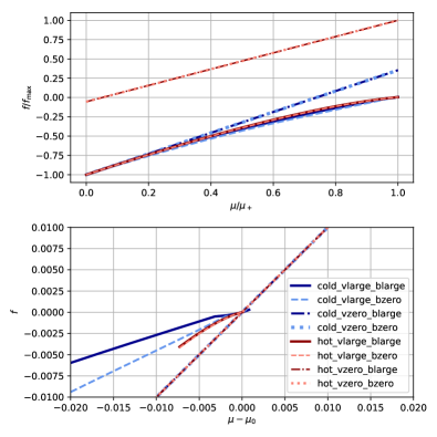
Figure 1: Master function $f$ for different regimes, combining: velocities $v=0$ and $v=0.99$ (labeled vlarge), magnetic field scale $b=0$ and $b=2$ (blarge), internal specific energy $\epsilon_{th}=0$ (cold) and $10$ (hot), where $\epsilon_{th}$ denotes the difference to the zero temperature case. Velocities are oriented orthogonally to the magnetic field, which is the most difficult case. In the top panel, the independent variable $\mu$ is scaled to the initial root bracket $\mu_{+}$, and the function is scaled to the maximum value over the interval shown. The lower panel shows the behavior near the root $\tilde{\mu}_{0}$.

II.6 Existence of solution

In the following, we prove that the master function always has a root, not just for valid evolved variables, but also for invalid ones. To this end, we construct an interval over which the master function changes sign. We start by defining an auxiliary function

$$f_{a}(\mu) =\mu\sqrt{h_{0}^{2}+\mathrm{bar}{r}^{2}(\mu)}-1$$ (49)

This is a smooth function which does not require evaluation of the EOS, using only the EOS-specific global lower enthalpy bound $h_{0}$. It is easy to show that $f_{a}$ is strictly increasing and has exactly one root $\mu_{+}$ in the interval $(0,h_{0}^{-1}]$. We will show that $\mu_{+}$ constitutes an upper bound for the root of the master function $f$. For $f_{a}(\mu_{+})=0$, we find

$$\begin{split}\mu_{+}\mathrm{bar}{r}(\mu_{+})&=\frac{\mathrm{bar}{r}(\mu_{+})}{\sqrt{h_{0}^{2}+\mathrm{bar}{r}^{2}(\mu_{+})}}\\ &\leq\frac{r}{\sqrt{h_{0}^{2}+r^{2}}}=v_{0}\,,\end{split}$$ (50)

where we used $r\geq\mathrm{bar}{r}$ and the monotonicity of the above expression with respect to $\mathrm{bar}{r}$. From Eq. (40), we find $\hat{v}(\mu_{+})=\mu_{+}\mathrm{bar}{r}(\mu_{+})\leq v_{0}<1$. Further, $f_{a}(\mu_{+})=0$ implies that

$$\mu_{+}h_{0} =\sqrt{1-\hat{v}^{2}(\mu_{+})}=\hat{W}^{-1}(\mu_{+})$$ (51)

Using the definition Eq. (48) of $\hat{\nu}$, which implies $\hat{\nu}\geq\nu_{A}$, we can write

$$\mu_{+}\hat{\nu}(\mu_{+}) \geq\mu_{+}\frac{\hat{h}(\mu_{+})}{\hat{W}(\mu_{+})}\geq\mu_{+}\frac{h_{0}}{\hat{W}(\mu_{+})}$$ (52)

$$=\hat{W}^{-2}(\mu_{+})=1-\mu_{+}^{2}\mathrm{bar}{r}^{2}(\mu_{+})$$ (53)

Hence,

$$1 \leq\mu_{+}\left(\hat{\nu}(\mu_{+})+\mathrm{bar}{r}^{2}(\mu_{+})\mu_{+}\right)=\mu_{+}/\hat{\mu}(\mu_{+})$$ (54)

Using the definition of the master function, Eq. (44), we find that $f(\mu_{+})\geq 0$, and, trivially, $f(0)<0$. Since $f$ is continuous, it has at least one root in the interval $(0,\mu_{+}]$. From Eq. (52), we also find that the root is strictly below $\mu_{+}$ unless $\hat{h}(\mu_{+})=h_{0}$.

Conveniently, the interval provides a useful initial bracketing for the root finding algorithm. Although finding $\mu_{+}$ requires another numerical root solving, the computation of $f_{a}$ does not require the expensive evaluation of the EOS. Moreover, determining $\mu_{+}$ is not required if $r<h_{0}$. In this case, $\hat{v}(1/h_{0})<1$ and $f_{a}(1/h_{0})>0$, hence one can safely use $(0,1/h_{0}]$ to bracket the root.

The main reason to expend this effort is to ensure that $\hat{v}\leq v_{0}<1$. Beyond $\mu_{+}$, the cutoff in Eq. (40) can induce a strong kink in the master function, reducing efficiency of the main root finding. With the tight upper limit $\mu_{+}$, the only reason for the cutoff is to make absolutely certain that not even rounding errors in ultra-relativistic cases can lead to not-a-number results. Finally, being able to use $\hat{v}\leq v_{0}$ simplifies the uniqueness proof in the next section.

II.7 Uniqueness of solution

Uniqueness of physically valid solutions is obviously important for any evolution scheme based on the conserved variables considered in this work. For the purpose of our recovery scheme, we require in addition that (i) for valid evolved variables, the master function has no additional roots corresponding to invalid solutions, and (ii) for invalid evolved variables, it still has exactly one root. In this section, we will prove that the above conditions are met.

We first compute the derivative of the master function. Differentiation and straightforward algebraic computations yield

$$\frac{\mathrm{d}x}{\mathrm{d}\mu} =-x^{2}b^{2}$$ (55)

$$\frac{\mathrm{d}\mathrm{bar}{r}}{\mathrm{d}\mu} =-\frac{(1-x)x^{2}}{\mu\mathrm{bar}{r}}r_{\bot}^{2}$$ (56)

$$\frac{\mathrm{d}\mathrm{bar}{q}}{\mathrm{d}\mu} =-(1-x)x^{2}r_{\bot}^{2},$$ (57)

$$\frac{\mathrm{d}}{\mathrm{d}\mu}(\mu\mathrm{bar}{r}(\mu)) =\frac{1}{\mathrm{bar}{r}}\left(x^{3}r_{\bot}^{2}+r_{\|}^{2}\right)\geq 0$$ (58)

Since $\mu\mathrm{bar}{r}(\mu)$ is monotonically increasing and we have shown in Sec. II.6 that $\mu_{+}\mathrm{bar}{r}(\mu_{+})\leq v_{0}$, it follows that for $\mu\leq\mu_{+}$, Eq. (40) reduces to $\hat{v}(\mu)=\mu\mathrm{bar}{r}(\mu)$. From this, we find

$$\frac{\mathrm{d}}{\mathrm{d}\mu}\ln(\hat{W}) =\hat{W}^{2}\mu\left(x^{3}r_{\bot}^{2}+r_{\|}^{2}\right)$$ (59)

In the following, we assume that the density $\mathrm{bar}{D}/\hat{W}$ does not leave the allowed range of the EOS. This corner case is discussed in Appendix A. We then obtain

$$\frac{\mathrm{d}}{\mathrm{d}\mu}\ln(\hat{\rho}) =-\frac{\mathrm{d}}{\mathrm{d}\mu}\ln(\hat{W})$$ (60)

So far, we have computed derivatives of quantities that do not depend on Eq. (42) and therefore we did not need to consider the limiting of $\epsilon$ to the valid EOS range. For the derivative of $\hat{\epsilon}$, we first consider the case in which $\epsilon$ computed by Eq. (42) is in the valid range. We then find

$$\frac{\mathrm{d}}{\mathrm{d}\mu}\hat{\epsilon} =\left(1+\hat{\epsilon}-\frac{1}{\hat{W}\mu}\right)\frac{\mathrm{d}}{\mathrm{d}\mu}\ln(\hat{W})$$ (61)

At a solution, $\mu\hat{W}\hat{h}=1$, and we obtain

$$\frac{\mathrm{d}}{\mathrm{d}\mu}\hat{\epsilon} =-\frac{\hat{P}}{\hat{\rho}}\frac{\mathrm{d}}{\mathrm{d}\mu}\ln(\hat{W})=\frac{\hat{P}}{\hat{\rho}^{2}}\frac{\mathrm{d}}{\mathrm{d}\mu}\hat{\rho}$$ (62)

This means that changes of density $\hat{\rho}$ and specific energy $\hat{\epsilon}$ are adiabatic when varying $\mu$ near a solution, i.e. the derivative of specific entropy $\hat{s}$ is zero. For the case in which $\epsilon$ computed by Eq. (42) is below the valid range of the EOS, $\hat{\epsilon}$ is set to the lower bound of the validity range, $\epsilon_{\text{min}}(\hat{\rho})$, which is the zero temperature limit according to our EOS requirements. Consequently, $\hat{\rho}(\mu)$ and $\hat{\epsilon}(\mu)$ follow a curve of constant $s$. In both of the above cases we can therefore compute the derivative of $\hat{h}$ using the adiabatic soundspeed given by Eq. (8) and the derivative of density given by Eq. (60), obtaining

$$\frac{\mathrm{d}}{\mathrm{d}\mu}\ln{\hat{h}} =-\hat{c}_{s}^{2}\frac{\mathrm{d}}{\mathrm{d}\mu}\ln{\hat{W}}$$ (63)

where $\hat{c}_{s}=c_{s}(\hat{\rho},\hat{\epsilon})$. In both cases, $\hat{\nu}=\hat{\nu}_{A}=\hat{h}/\hat{W}$, and we find

$$\frac{\mathrm{d}}{\mathrm{d}\mu}\ln{\hat{\nu}} =-\left(1+\hat{c}_{s}^{2}\right)\frac{\mathrm{d}}{\mathrm{d}\mu}\ln{\hat{W}}\,,$$ (64)

At a solution, the derivative of the master function becomes

$$\begin{split}\frac{\mathrm{d}}{\mathrm{d}\mu}f(\mu)&=1-\hat{v}^{2}+\hat{v}^{2}\left(1-c_{s}^{2}\right)\frac{x^{3}r_{\bot}^{2}+r_{\|}^{2}}{\mathrm{bar}{r}^{2}}\\ &\geq 1-\hat{v}^{2}>0\end{split}\,,$$ (65)

as shown in Appendix A. The requirement $c_{s}<1$ is therefore sufficient to guarantee uniqueness of the root for all velocities and magnetic fields. Note that for superluminal soundspeeds, we cannot prove uniqueness unless $v^{2}c_{s}^{2}<1$. In that case, the proof of existence still holds, but is is not known if the physical solution becomes ambiguous.

So far, we have not addressed the corner case where the specific energy is above the valid range of the EOS. In that case, $\hat{\nu}$ is computed from Eq. (47). A straightforward computation (see Appendix A) reveals that uniqueness is always ensured under the condition that

$$\frac{A(\rho)}{1+\hat{a}}\frac{\partial a}{\partial\epsilon}\leq 1-c_{s}^{2}$$ (66)

The function $A$ is defined by the relation

$$\frac{A(\rho)}{\rho} =\frac{\mathrm{d}}{\mathrm{d}\rho}\epsilon_{\text{max}}(\rho)-\frac{P}{\rho^{2}}$$ (67)

It is related to the change of specific entropy along the upper validity range $\epsilon_{\text{max}}$ of the EOS. For $A=0$, the equation above reduces to the thermodynamic condition for adiabatic change. The condition given by Eq. (66) does not seem to be very restrictive. If in doubt, one can always use a boundary with $A=0$ (constant specific entropy) to guarantee uniqueness in all cases. In practice, we encountered no problems using upper validity bounds defined by either constant temperature or constant $\epsilon$.

II.8 Guaranteed accuracy

Since the root of the master function is determined numerically, we require a criterion to stop the iteration once sufficient accuracy is reached. What is sufficient depends on the other errors present in a numerical evolution scheme. We will discuss evolution errors in Sec. V. In this section, we discuss the error propagation of the root finding accuracy to quantify the accuracy of the recovered primitives.

However, we first need to specify how the final result is computed from the outcome of the last root finding iteration. This involves a design decision, since the available variables $\mu,\hat{\mu},\hat{\nu},\mathrm{bar}{r},\mathrm{bar}{q},\hat{v},\hat{W},\hat{\rho},\hat{\epsilon},\hat{h},\hat{P}$ allow us to compute the primitives in many different ways, which lead to different error propagation. Here, we use $\hat{W},\hat{\epsilon},\hat{\rho},\hat{P}$ directly, which turns out to be a good choice in terms of error propagation. To reconstruct the velocity vector, we use the expression

$$\hat{v}^{i} =\mu\mathrm{bar}{r}^{i}=\mu x\left(r^{i}+\mu\left(b^{l}r_{l}\right)b^{i}\right)\,,$$ (68)

which is just Eq. (29) rearranged to avoid degeneracy for the case $b=0$. It is easy to verify that the Lorentz factor $W(\hat{v}^{2})$ corresponding to Eq. (68) is exactly $W(\hat{v}^{2})=\hat{W}$. Since $\hat{\rho}=D/\hat{W}$, the conserved density $\hat{D}=\hat{\rho}W(\hat{v}^{2})$ computed from the recovered primitive variables $\hat{\rho},\hat{v}^{i}$ agrees exactly with the original one.

In the following, we only consider the case where the solution is in the validity region of the EOS. For invalid solutions, the accuracy of the solution is less relevant since in this case the cause is the evolution error and the result will either be corrected to the valid range or the simulation aborted. The error introduced by such corrections will be discussed in Sec. V.4.

Assuming the root of $f(\mu)$ was determined numerically to an accuracy of $\delta\mu$, we now estimate the resulting accuracy of the primitive variables to linear order, computing, e.g., ${\delta\hat{W}=\delta\mu\,\mathrm{d}\hat{W}/\mathrm{d}\mu}$. We already evaluated the first derivatives at a root of $f$ in Sec. II.7. From those, we obtain

$$\frac{\delta\hat{W}}{\hat{W}} \leq\hat{v}^{2}\Delta\,, \Delta \equiv\hat{W}^{2}\frac{\delta\mu}{\mu}$$ (69)

$$\frac{\delta\hat{z}}{\hat{z}} \leq\Delta\,, \frac{\delta\hat{v}}{\hat{v}} \leq\frac{|\delta\hat{v}^{i}|}{\hat{v}}\leq\frac{\Delta}{\hat{W}^{2}}$$ (70)

$$\frac{\delta\hat{\rho}}{\hat{\rho}} \leq\hat{v}^{2}\Delta\,, \frac{\delta\hat{h}}{\hat{h}} \leq\hat{v}^{2}\Delta$$ (71)

$$\frac{\delta\hat{\epsilon}}{1+\hat{\epsilon}} \leq\hat{a}\hat{v}^{2}\Delta\,, \frac{\delta\hat{\epsilon}}{\hat{\epsilon}} \leq\left(1+\hat{\epsilon}\right)\frac{\hat{a}}{\hat{\epsilon}}\hat{v}^{2}\Delta$$ (72)

$$\frac{\delta\hat{\rho_{E}}}{\hat{\rho_{E}}} \leq 2\Delta\,, \frac{\delta\hat{P}}{\hat{P}} \leq\hat{v}^{2}\left(1+\hat{a}\right)\frac{\hat{c}_{s}^{2}}{\hat{a}}\Delta\,,$$ (73)

where $|\delta\hat{v}^{i}|$ denotes the norm given by the 3-metric of the vector $\delta v^{i}$. The error in the recovered primitive variables corresponds to errors $\delta q,\delta S_{i}$ of conserved variables. We estimate these errors to linear order, by inserting $\hat{\rho},\hat{h},\hat{P},\hat{v}^{i}$ into equations (15–20) and (21) and then evaluate the first derivatives with respect to $\mu$ at the root. We obtain the following scaling

$$\frac{|\delta S_{i}|}{|S_{i}|} \leq\Delta\,, \frac{\delta(1+q)}{1+q} \leq 4v^{2}\Delta$$ (74)

We find that the accuracy in $\mu$ required for a fixed relative error of the primitives increases with increasingly relativistic velocities. On the other hand, the magnetic scale $b$ has no impact on the error bounds. It is also worth noting that the error $\delta s$ of the the specific entropy $s$ is zero (to linear order in $\delta\mu$) because the variation of $\hat{\rho},\hat{\epsilon}$ with respect to $\mu$ is adiabatic (see Sec. II.7). Finally, we note that the above error bounds do not include numerical rounding errors. Those will be discussed in Sec. IV.2.

III Enforcing Validity

In typical numerical simulations, the evolved magnetohydrodynamic variables frequently reach an invalid state at some points, mainly due to ordinary numerical error, but also external influences such as gauge pathologies near the centers of newly formed black holes. Often, such violations are harmless and can be corrected. Any such correction turns unphysical conditions into regular evolution errors, and obviously different prescriptions will lead to different errors, both in magnitude and in character. Although correcting violations should be regarded as part of the evolution scheme, some basic point-wise corrections can be incorporated into the primitive recovery code, granting it power to change the evolved variables. The following effects cause typical harmless violations:

1. When evolving zero-temperature initial data, arbitrary small evolution errors can lead to evolved variables that correspond to a fluid energy density below the zero-temperature limit.

2. At numerical grid points at the surface of neutron stars moving through vacuum, mass and energy densities during a single timestep can drop by orders of magnitude or even become negative. Although the absolute errors of the conserved variables remain small compared to the global scales of the system, the resulting local error of the specific internal energy and velocity can become huge and lead to an invalid state. The effect is alleviated over time because the errors tend to heat the outermost layer of NS surface, creating a hot atmosphere that reduces the density gradient.

3. During collapse to a black hole, mass density and/or temperature might leave the range covered by the given EOS, arriving at a state that is not unphysical but cannot be evolved further. This typically occurs in regions already inside the horizon or about to be engulfed by a rapidly expanding apparent horizon.

4. The coordinates near a black hole center are strongly stretched for gauges like the puncture gauge, and the surroundings are extremely under-resolved numerically. Under those conditions, all kinds of numerical instabilities can occur for the combined magnetohydrodynamical and spacetime evolution system.

III.1 Simple corrections

By design, our primitive variable recovery scheme is able to deal also with invalid input. As a side-effect, we obtain a projection onto the valid regime, by simply recomputing the evolved variables from the recovered primitives. As described in Sec. II.5, the scheme always yields a pair $\hat{\rho},\hat{\epsilon}$ such that $\hat{\epsilon}$ is within the validity range of the EOS at $\hat{\rho}$.

We first consider the important case in which the raw value of $\epsilon$ is below the valid range. In this case, only the recomputed conserved energy $\tau$ changes, while $S$ and $D$ stay the same. This can be seen as follows. The only variable through which the adjustment of $\epsilon$ to the valid range impacts the master function is $\hat{\nu}$. For the case at hand, Eq. (48) implies $\hat{\nu}=\nu_{A}$. Furthermore, the conserved energy $\tau$ enters exclusively through Eq. (42). Therefore, if $\tau$ is adjusted such that Eq. (42) yields the range-limited value for $\hat{\epsilon}$, we arrive at the same primitive variables without adjustment.

For the case in which the energy is above the validity range of the EOS, all recomputed conserved variables can change. One could prevent this by always using $\hat{\nu}=\nu_{A}$, but not without changing the behavior of the master function away from the solution. However, this case is less important, because this correction should only be allowed at low-density fluid-vacuum boundaries (NS surfaces) or inside horizons.

In the interiors of black holes, it becomes necessary to employ a more lenient error policy than outside. Although physical effects cannot propagate out of the horizon, violations of the constraint equations and gauge effects impact the exterior. Therefore, one cannot allow any runaway instability inside the horizon. For the matter part, this mainly concerns energy and momentum, since the total baryon number is conserved in finite volume schemes (artificial atmosphere corrections aside), and the mass density remains finite. The energy can be limited by allowing the aforementioned correction to the EOS range inside horizons even at high densities.

This leaves the momentum. For pure hydrodynamic simulations, limiting the velocity proved effective to prevent runaway instabilities near the BH center. This was employed for the simulations in Galeazzi et al. (2013), by rescaling the velocity to stay within a given limit. For MHD simulations, this approach has a side-effect. Since the reconstructed electric field depends on the velocity via Eq. (21), it will also change. That might be problematic or not, depending on the evolution scheme. The evolution of the EM field might be problematic in this regime in any case. However, addressing such problems is clearly not inside the scope of the primitive variable recovery, since it operates point-wise and cannot change electric or magnetic fields in any reasonable way.

Another correction often applied is to enforce a minimum mass density, also called artificial atmosphere. There are two motives. One is the wish to use a tabulated EOS that does not include zero density (this might be achieved more consistently by extending the range to zero via analytic expressions). The more fundamental motive is that the hydrodynamic evolution equations break down in vacuum. In purely hydrodynamic simulations, it is common to set the atmosphere velocity to zero with respect to the simulation’s coordinate system, in order to prevent an unphysical influx of matter. In ideal MHD simulations, the situation is more complicated because the electric field is tied to the velocity via Eq. (21). Therefore, the atmosphere velocity prescription should be the domain of the evolution scheme and not of the primitive recovery.

IV Performance

In the following we assess how well our scheme performs in practice. For this, we subject a reference implementation to a series of numerical tests. These stand-alone tests simulate conditions relevant for the future use of the scheme in actual numerical simulation codes.

Our tests aim to validate that the following requirements are met. First, the scheme should not fail to converge for any input we expect to occur in numerical simulations of binary neutron star mergers (or supernova core collapse, which has similar demands). Second, within the physical regimes that may occur in the above scenarios, the errors caused by the primitive recovery should be insignificant compared to the ones caused by modern evolution schemes.

Lorentz factor $W$, magnetic scale $b$, and specific energy $\epsilon$ are the most important variables governing the behavior of the primitive recovery. To get an indication of what values to expect for $b$, we consider the merger simulations described in Ciolfi et al. (2017, 2019) as a typical use case. The maximum magnetic field strength reached after the merger by various amplification mechanisms is ${\sim}10^{17}\usk\mathrm{G}$. The lowest density reached in the funnel along the axis after black hole formation is around ${\sim}10^{8}\usk\mathrm{g}\mathrm{/}\mathrm{c}\mathrm{m}\mathrm{{}^{3}}$, although these conditions do not coincide.

The corresponding value $b\approx 100$ constitutes a reasonable scale up to which we demand robustness. A comparable value $b\approx 30$ corresponds to initial data with neutron stars possessing a magnetar-like exterior field strength $10^{15}\usk\mathrm{G}$ that extends into an artificial atmosphere with typical densities $10^{5}\usk\mathrm{g}\mathrm{/}\mathrm{c}\mathrm{m}\mathrm{{}^{3}}$. In merger simulations, the regions with magnetic fields amplified even further do not overlap with the lowest density regions. Combining a field ${\sim}10^{17}\usk\mathrm{G}$ with the aforementioned artificial atmosphere density, we find that $b\approx 10^{3}$ exceeds practical use cases by far and demanding robustness up to this scale is not required.

Although the typical Lorentz factors we encounter in merger simulations are well below 10, one motivation for magnetized merger simulation is to observe the launch of a jet, and future applications might follow up such a jet to higher Lorentz factors. High Lorentz factors might also appear inside black holes. Therefore, we demand robustness up to $W=10^{3}$.

Regarding the requirements for specific energy, we note that nuclear matter at the highest densities possible in NSs can reach $\mathcal{O}(\epsilon)=1$ at zero temperature. Although temperatures can easily reach ${\sim}50\usk\mathrm{MeV}$ inside merging NS (see Kastaun et al. (2016) for example), this happens at high densities. The thermal contribution to $\epsilon$ stays well below unity (see, e.g., the appendix of Endrizzi et al. (2018)). Furthermore, for states with $\epsilon\gg 1$, the energy of the photon gas dominates that of baryonic matter, and the evolution equations of magnetohydrodynamics are not applicable anymore. It seems reasonable to demand accuracy and robustness of the primitive recovery up to $\epsilon\approx 10$.

In order to understand finite precision effects, we compare the accuracy that our reference implementation reaches to the expected accuracy derived in Sec. II.8, using a value $\Delta=10^{-8}$. We assume that such an accuracy is negligible compared to the evolution error. Note, however, that in Sec. V, we show that the accuracy of $\epsilon$ (and hence $P$) related to the accuracy of the evolved variables deteriorates quickly for $b>1$, with a factor $\approx b^{2}/\epsilon$. We therefore restrict tests of primitive recovery accuracy to the regime $b<5$ and caution that one cannot trust the evolution scheme at higher values.

IV.1 Code Design

We created a reference implementation for the algorithm described in Sec. II. A schematic summary of the algorithm is given in Fig. 2. We provide our reference implementation in the form of a C++ library named RePrimAnd. The library is not tied to any particular evolution framework, allowing the use in arbitrary evolution codes. It also contains a framework providing access to different types of EOS through a generic interface, ensuring that the user code (such as our primitive recovery code) is completely EOS-agnostic. The generic interface also provides the EOS validity ranges and rigidly enforces our EOS requirements (see Sec. II.2). The reference implementation is publicly available Kastaun (2020).

Our library provides different EOS types (not yet including fully tabulated ones) including a hybrid EOS based on a tabulated cold part. Although the MS1 variant from Read et al. (2009) used for our test is given analytically in the form of piecewise polytropic expressions, we evaluate it in our tests as a tabulated cold part, in order to test the general purpose code intended for production runs. We set the allowed range of the EOS to $\rho_{\mathrm{max}}=3\times 10^{15}\usk\mathrm{g}\mathrm{/}\mathrm{c}\mathrm{m}\mathrm{{}^{3}},\epsilon_{\mathrm{max}}=51$.

In order to find the root of the master function, our implementation uses the TOM748 algorithm Alefeld et al. (1995) provided by the BOOST library. This root finding scheme is similar to the well known Brent-Dekker schemes, but it uses inverse cubic instead of quadratic interpolation whenever possible, improving convergence speed near the solution. It keeps the solution enclosed in a bracket, with extent converging in a limited amount of steps, and it does not make use of function derivatives. The motivation for avoiding derivatives is that, in practice, tabulated EOS tend to have very inaccurate partial derivatives, which is problematic when using a derivative-based root solver such as Newton-Raphson. Our implementation therefore does not make use of the soundspeed or other derivatives. The root is determined to an accuracy specified by prescribing $\Delta$ defined in Eq. (69), where the error $\delta\mu$ is taken as the size of the current tightest bracket of the root.

In the case where $r\geq h_{0}$, we need to determine $\mu_{+}$ from the root of the auxiliary function $f_{a}$, for which we employ a standard Newton-Raphson root solver. This is unproblematic since $f_{a}$ is a smooth, monotonic, analytic function. We determine $\mu_{+}$ to an accuracy close to machine precision, and then increase $\mu_{+}$ by a multiple of the root solving accuracy to ensure the root of the master function is really contained.

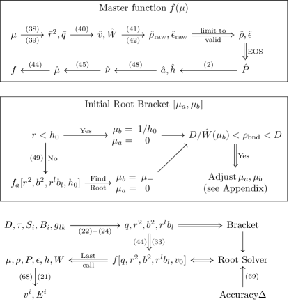
Figure 2: Schematic overview of the recovery algorithm information flow and list of required equations. Arrows denote dependencies, including variables further up in the chain. Double arrows denote computations that require information about the EOS validity bounds, the one double arrow labeled “EOS” refers to evaluation of the EOS. Intermediate results obtained during evaluation of the master function in the last root finding iteration are denoted “Last call”. Square brackets refer to the list of fixed parameters (independent of $\mu$) during root solving. The density $\rho_{\text{bnd}}$ stands for any one of the upper and lower EOS validity bounds.

IV.2 Robustness and Accuracy

Our main test validates both robustness and expected accuracy, by sampling the primitive variable parameter space given by density, temperature/specific energy, magnetic scale $b$, and velocity. We sample $z=Wv$ between $0$ and $1000$, magnetic scale $b$ from $0$ to $5$, and the specific thermal energy from $\epsilon_{\mathrm{th}}=10^{-4}$ up to $50$. For the MS1 EOS, we sample the mass density from $10^{6}$ to $10^{15}\usk\mathrm{g}\mathrm{/}\mathrm{c}\mathrm{m}\mathrm{{}^{3}}$. For the ideal gas EOS, the mass density is irrelevant due to the scaling behavior of the EOS. We use two orientations of the velocity, parallel and orthogonal to the magnetic field. The tests are performed both for the ideal gas and for the hybrid EOS, described in Sec. II.2, and we demand an accuracy $\Delta=10^{-8}$.

We verify that the algorithm always, without any exception, succeeds in recovering the correct solution for the valid input described above. Moreover, we create test cases to assure that input corresponding to energy outside the range possible for a given EOS is correctly classified as such.

To assess the accuracy, we compute the conserved variables from the primitives, apply the primitive recovery algorithm, and compare the result to the original primitives. Further, we compute the conservatives from the recovered primitives and compare them to the original conservatives. Our testsuite compares the observed accuracy for each individual primitive variable to the one expected from Eq. (69) to Eq. (73), and also the accuracy of the corresponding conserved variables to Eq. (74). When demanding an accuracy better than $\Delta\lesssim 10^{-7}$, those bounds are exceeded either for high Lorentz factors or very small $\epsilon$ and $v$. We attribute the excess error to various rounding errors.

We identify the most important rounding errors as follows. First, the master function is the difference of two values which can each be expressed only to machine precision. To get the impact on the root, we have to divide by the derivative of the master function, which in this case satisfies $f^{\prime}\leq 1-v^{2}c_{s}^{2}$. At the same time, we demand an accuracy $\Delta/W^{2}$. For the highly relativistic case $W=10^{3}$ and around 16 digits machine precision, this limits $\Delta>10^{-10}$. If the soundspeed approaches unity, the accuracy is further limited. Second, $\epsilon$ is computed by subtracting kinetic and magnetic energy density from the total one. If $\epsilon$ is small compared to these, the cancellation error causes a loss of significant digits. Analyzing Eq. (42), we find additional rounding errors of magnitudes $z^{2}/\epsilon$ and $b^{2}W/\epsilon$ worse than machine precision.

Taking into account both the regular errors predicted by Eq. (69) to Eq. (73) as well as the main rounding errors discussed above, the recovered accuracy is quantitatively within the expected bounds over the whole range of our test cases. Fig. 3 shows the recovered accuracy for the pressure as well as the boundary where the errors caused by rounding start exceeding those caused by root finding.

We do not expect rounding errors to be of practical importance. The rounding errors at low $\epsilon,v$ are very small and only dominate because the regular errors approach zero. The rounding errors in the ultra-relativistic/highly magnetized regime are still not prohibitive, but will be dominated by the errors of the time evolution, which will be discussed in Sec. V.

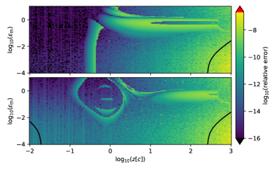
Figure 3: Relative error of reconstructed pressure, as a function of specific thermal energy and velocity (the latter in terms of $z=Wv$). The results were obtained for the case of the hybrid EOS (see text), at fixed mass density $6\times 10^{12}\usk\mathrm{g}\mathrm{/}\mathrm{c}\mathrm{m}\mathrm{{}^{3}}$, demanding an accuracy $\Delta=10^{-8}$. The upper panel shows results for zero magnetic field, and the lower panel for the magnetically dominated case $b=10$. The solid lines mark the regions where expected errors related to rounding start to exceed those related to root solving.

IV.3 Efficiency

In the following, we discuss the efficiency of our scheme on the level of the algorithm, while reserving benchmarks of the execution speed of the implementation within actual GRMHD simulations for future work. We measure the computational efficiency of our algorithm in terms of calls to the EOS. The motivation is that for a tabulated EOS including thermal and composition degrees of freedom, a single EOS call is likely more expensive than the evaluation of the analytic expressions within our recovery scheme. The worst scenario is when the EOS is tabulated with temperature as one independent variable. Each EOS call then requires an inversion step to convert from $\epsilon$ to $T$.

Fig. 4 shows how the efficiency varies with specific energy and velocity, either for zero magnetic field, or with magnetic scale fixed to a large value of $b=10$. We find that the efficiency does not degrade even for Lorentz factors up to 1000 and magnetic scales up to $b=10$. At the density shown, $b=10$ corresponds to extremely high magnetizations of orders $10^{4}$ (for $W=1$) to $10^{7}$ (for $W=1000$).

When considering the whole parameter space used in the unit tests (not just the cuts shown in the plots) and both EOS types, we find a maximum number of 23 calls to the EOS required to achieve an accuracy $\Delta=10^{-8}$. The maximum occurs for the ideal gas and only when both $\epsilon>40$ and $b>2$, i.e., thermal energies much larger and magnetic energies larger than the rest mass density.

In Fig. 5, we show the efficiency with respect to velocity and magnetic scale $b$, taking the latter up to extreme values $b=10^{4}$, far beyond any reasonable use case. We find that beyond $b=10$, the efficiency gradually starts to decrease. At $b=10^{4},W=10^{3}$, we require around 40 steps for $\Delta=10^{-8}$ (which implies $\delta\mu/\mu\approx 10^{-14}$). At this point, the root solving convergence speed has decreased roughly to that of bisection. Still, we encounter no failures to converge even in this range.

Note that the extremes reached in our tests are rather pathological scenarios which are rarely encountered in simulations and are therefore not relevant for numerical costs of simulations. In practice, we expect an average number of required calls below 10.

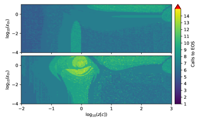
Figure 4: Number of calls to the EOS required to reconstruct the primitives to accuracy $\Delta=10^{-8}$, as a function of specific thermal energy and velocity (in terms of $z=Wv$). The results were obtained for the case of the hybrid EOS (see text) at a mass density $\rho=6\times 10^{12}\,\mathrm{g}\mathrm{/}\mathrm{c}\mathrm{m}\mathrm{{}^{3}}$. The upper panel shows results for the magnetic scale $b=0$, and the lower panel for the magnetically dominated case $b=10$.

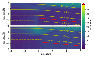
Figure 5: Number of calls to the EOS required to reconstruct the primitives to accuracy $\Delta=10^{-8}$, as a function of magnetic scale $b$ and velocity (in terms of $z=Wv$). The results were obtained for the case of the hybrid EOS (see text) at a mass density $\rho=6\times 10^{12}\,\mathrm{g}\mathrm{/}\mathrm{c}\mathrm{m}\mathrm{{}^{3}}$. The upper panel shows results for cold matter $\epsilon_{\text{th}}=10^{-4}$, and the lower panel for very hot matter $\epsilon_{\text{th}}=10$. For comparison, we also show the magnetization as contour lines of $\log_{10}(B^{2}/P)$. The red line marks a magnetic field strength $B=10^{16}\usk\mathrm{G}$.

IV.4 Comparison with other schemes

In the following, we compare our scheme to existing ones. We refer to Siegel et al. (2018) for a comprehensive review and numerical tests of previous schemes. The main characteristics are listed in Table 1.

One important difference is the number of independent variables. Most of the existing schemes need to solve an equation in two or three unknowns. This is a severe drawback. First, it is difficult to ensure that the solution is found. The Newton-Raphson (NR) schemes might not converge. Second, robust but fast schemes that guarantee finding the solution in a limited number of steps only exist for one-dimensional root finding. Third, the recovery schemes based on NR require an initial guess, which is typically taken from the previous timestep during numerical evolution. This makes the methods more unpredictable and more difficult to test, as they do not depend on the conserved variables in a deterministic way. As two of the existing schemes, our scheme is using one-dimensional root finding. Further, it also makes use of a tight initial bracketing interval proven to contain exactly one solution.

As demonstrated in Siegel et al. (2018) all of the existing schemes can fail for Lorentz factors 10–1000, depending on the magnetization. Fig. 3 of Siegel et al. (2018) shows the number of iterations or failure to converge as function of magnetization and Lorentz factor, at fixed density $10^{11}\usk\mathrm{g}\mathrm{/}\mathrm{c}\mathrm{m}\mathrm{{}^{3}}$ and $T=5\usk\mathrm{MeV}$ (thus $\epsilon<1$). For our scheme, $b$ is the most relevant measure for the magnetic field (but not necessarily for the other schemes). For comparison, the magnetization $10^{10}$ covered in the figure corresponds to values up to $b\approx 10^{4}$. As argued before, such values are outside the parameter space relevant for use in merger simulations. Therefore, the failures at low velocity, but with magnetization around $10^{9}$ shown in Fig. 3 of Siegel et al. (2018) are not problematic in practice. The fact that our scheme showed no failure at $b=10^{4}$ for the test shown in Fig. 5 is however reassuring regarding the numerical robustness. The failures at relativistic velocities for lower magnetization shown in Fig. 3 of Siegel et al. (2018) should however be regarded as problematic. For our algorithm, the existence and uniqueness of the solution are proven analytically, and we successfully test our numerical implementation up Lorentz factors $W=1000$ in the whole parameter space described in Sec. IV.2.

Strong magnetization is important for studying the engine of short gamma-ray bursts (SGRBs), where ideally a very low density matter is subject to very strong magnetic fields. This regime is also problematic for the numerical time evolution itself. The ability of our scheme to distinguish reliably between valid and invalid evolved variables is therefore an important advantage.

Fig. 2 of Siegel et al. (2018) shows the average of the relative errors (called $\mathrm{bar}{\sigma}$ in the following) for $\rho,v^{i},\epsilon$ as a function of temperature and density, for fixed low magnetization $p_{\mathrm{mag}}/p=10^{-3}$ and Lorentz factor $W=2$. We note that for the nuclear physics EOS, one can ignore the top-left part of the plots in Fig. 2, because this low-density, high-temperature regime corresponds essentially to a photon gas not relevant for practical use. Using the energy density $\rho_{\gamma}\propto T^{4}$ of a photon gas, we find that the bound $\epsilon<10$ used in our tests corresponds to temperatures below a straight line (in the log-log plot) through $(10^{12}\usk\mathrm{g}\mathrm{/}\mathrm{c}\mathrm{m}\mathrm{{}^{3}},10^{12}\usk\mathrm{K})$ and $(10^{4}\usk\mathrm{g}\mathrm{/}\mathrm{c}\mathrm{m}\mathrm{{}^{3}},10^{10}\usk\mathrm{K})$. For the ideal gas EOS, the temperature is instead defined assuming only baryons, such that $\epsilon<1$ throughout the figure.

In most of the physically relevant region, the recovery accuracy shown in Siegel et al. (2018) seems more than sufficient for use in evolution schemes. However, some existing schemes exhibit isolated regions where the accuracy degrades inexplicably. This is worrisome since the figure shows only a mildly relativistic twodimensional cut in the parameter space, and there is no guarantee that the accuracy will not deteriorate intolerably elsewhere. In contrast, our scheme has the advantage of a theoretical model for the errors of each of the primitive variables, including the dominant finite precision errors. This model was validated for our numerical implementation over the full parameter space $(\rho,W,\epsilon,b)$ as described in Sec. IV.2.

Regarding the efficiency, the different tolerance measures allow only a rough comparison, using the number of root finding iterations shown in Figs. 1 and 3 of Siegel et al. (2018). Note that the top-left part of the plots in Fig. 1 is not practically relevant for the nuclear physics EOS, as discussed above. As mentioned before, the problems at the highest magnetizations $>10^{9}$ in Fig. 3 of Siegel et al. (2018) can be safely ignored for practical use. In case no failure occurs, only the Newman scheme appears to be consistently requiring less than around 10 steps also for relativistic velocities. The others need 30 iterations or more in certain regions of parameter space.

Our scheme is guaranteed to converge in a finite number of steps because the root finding algorithm performs bisection steps if needed. Our tests have shown that the efficiency does not degrade for large Lorentz factors ($W<1000$) or strong magnetization ($b<100$), in contrast to most other schemes. The worst case scenario for our scheme seems to be extreme values of $\epsilon$. Even for essentially photonic states ($\epsilon=50$), it does not require more than 23 EOS calls in the regime $b<5,W<1000$.

Up to this point, we considered the convergence criteria used during the iteration as an integral part of the different algorithms. Now we have to discuss if the different measures of success could bias the comparison. In Siegel et al. (2018), recovery was called successful when an average error $\mathrm{bar}{\sigma}<5\times 10^{-8}$ could be achieved. Comparing this to the root solving errors given by Eqs.(69) to (73), we find that $\mathrm{bar}{\sigma}<K\Delta$, where $K$ is a constant of order unity . However, the term $\delta\epsilon/\epsilon$ is also very sensitive to unavoidable cancellation errors, as already discussed in Sec. IV.2. Taking into account the finite floating point precision of $q,r,b$, we find that catastrophic cancellation decreases the number of valid digits for $\epsilon$ by around $\log_{10}(z^{2}/\epsilon)$ for the case $b=0,z^{2}\gg\epsilon$, and by $\log_{10}(b^{2}/\epsilon)$ for $v=0,b^{2}\gg\epsilon$. For the ideal gas case shown in the upper panel of Fig. 3 in Siegel et al. (2018), $\epsilon$ and $P$ are constant and one can easily estimate the loss of precision. Assuming a typical machine precision of 15 digits for $q,r,b$, rounding errors will make it impossible to reach the tolerance $\mathrm{bar}{\sigma}$ required in Siegel et al. (2018) at $W\gtrsim 2\times 10^{3}$ (for small $B$) or at $P/P_{\mathrm{mag}}\gtrsim 5\times 10^{8}$ (for small $v$). The above errors are a fundamental consequence of evolving the conserved variables, independent of the recovery scheme. Some, if not all of the “failures” near the upper boundary of the ideal gas panels are therefore inevitable, also for our scheme.

We test if our implementation can reach the $\mathrm{bar}{\sigma}$-tolerance from Siegel et al. (2018) within our standard test domain introduced in Sec. IV.2. In general, at $b=0$ our theoretical order of magnitude estimate predicts a larger impact of rounding errors for $\epsilon\lesssim 0.005\cdot(W/10^{3})^{2}$. For the ideal gas, the tolerance $\mathrm{bar}{\sigma}$ was indeed only reached when restricting $\epsilon$ above this estimate. Apart from this regime, the tolerance was reached in the whole standard test domain ($W\leq 10^{3},b<5$) using $\Delta=10^{-8}$. The same holds for the hybrid EOS. We conclude that the impact of the cancellation error on the error measure $\mathrm{bar}{\sigma}$ is close to the theoretical minimum for our implementation. In contrast, all schemes shown in Siegel et al. (2018) exceed the tolerance already below $W<10^{3}$ at small $B$, where our scheme succeeds.

The above discussion indicates that $\mathrm{bar}{\sigma}$ might not be a good choice as a criterion for recovery failures. We also point out that the relative error of $\epsilon$ is not a good measure for the error of the temperature, which is more closely related to the thermal part $\epsilon_{\mathrm{th}}$. For practical applications, it seems preferable to allow the inevitable accuracy loss for $\epsilon$ discussed above, recovering each primitive variable as accurately as theoretically possible. Whether or not the unavoidable cancellation errors in $\epsilon$ are tolerable surely depends on the application and should be regarded as part of the post-recovery error policy.

As is pointed out in Siegel et al. (2018), comparing the number of EOS calls between different schemes does not directly translate to numerical costs. The reason is that the schemes differ with respect to the required form of the EOS. Our scheme is using $P=P(\rho,\epsilon)$, while nuclear physics EOS tables are typically given in terms of $T$ instead of $\epsilon$. It was argued in Siegel et al. (2018) that it is advantageous if the master function directly uses the temperature as the independent variable, because otherwise each call to the EOS requires another root finding to determine $T$. We regard this as a shortcoming of the EOS implementation and advocate against basing the design of the primitive recovery on internals of specific EOS implementations. A more natural solution is to first create new tables in terms of $\epsilon$ (or a suitable analytic function thereof), by interpolating available nuclear physics tables. This allows one to choose the most robust recovery procedure without sacrificing speed. When using a lookup table based on temperature, however, the scheme proposed in Siegel et al. (2018) might indeed be faster than ours. We point out, however, that the large speedup discussed in Siegel et al. (2018) seems to be based on a particularly wasteful implementation of the inversion $T(\epsilon)$ that can require up to hundred steps. In Galeazzi et al. (2013), we used a discrete bisection in index space followed by inverse interpolation, which requires $<10$ steps for realistic table sizes.

In contrast to Siegel et al. (2018), we do not test the scheme with a fully tabulated EOS and can therefore make no conclusive claims on robustness and accuracy of the implementation in this case. However, the algorithm itself is guaranteed to find a solution. We recall that the proof of existence does not rely on EOS properties except for a lower bound on $h$. A table in conjunction with an interpolation method represents a well defined EOS. As long as this EOS respects the physical constraints listed in Sec. II.2, the uniqueness is also guaranteed. A careless implementation of a tabulated EOS that violates those constraints might however cause our algorithm to find wrong, unphysical solutions. For such faulty EOS there might even exist several physical solutions. Furthermore, our accuracy bounds are not guaranteed anymore because they rely on the constraints as well. Still, we do expect the numerical root finding to converge to a solution. Even jumps in the master function would only reduce the efficiency of the TOM748 solver, possibly down to that of bisection. We recall that this root finding method does not use derivatives, and would therefore not be affected by an EOS implementation returning inaccurate numerical derivatives of the pressure. Such inconsistencies might affect those schemes in Siegel et al. (2018) based on Newton-Raphson root solvers. However, the failures to converge exposed in Siegel et al. (2018) also appear for the purely analytic ideal gas EOS, and can therefore not be attributed to possible faults in EOS tables.

Table 1: Main characteristics of different recovery schemes. We list the independent variables used in the root finding (translated to our notation), the variables for which the EOS needs to be evaluated, whether the scheme requires derivatives of the EOS, whether the formulation allows a bound on the number of iterations needed for finding the solution, and whether the scheme requires to provide an initial guess for the solution.

Scheme	Independent	EOS	EOS	Steps	Guess
	variables	form	der.	bounded	needed
This work	$\mu$	$P(\rho,\epsilon)$	No	Yes	No
Noble Noble et al. (2006)	$(D/\mu,v^{2})$	$P(\rho,h)$	Yes	No	Yes
Siegel Siegel et al. (2018)	$(D/\mu,T)$	$P(\rho,T)$	Yes	No	Yes
Duran Cerdá-Durán et al. (2008)	$(W,D/\mu,T)$	$\epsilon(\rho,T)$	Yes	No	Yes
Neilsen Neilsen et al. (2014); Palenzuela et al. (2015)	$D/\mu$	$P(\rho,\epsilon)$	No	Yes	No
Newman Newman and Hamlin (2014)	$P$	$P(\rho,h)$	No	Yes	No

V Impact of Numerical Error in Evolved Variables

In the following, we investigate consequences of numerical errors in the evolved variables in conjunction with the corrections of invalid states described in Sec. III. Further, we identify regions in parameter space where the primitive variables are particularly sensitive to errors of the evolved ones.

V.1 Newtonian Limit

It is instructive to consider the relation between evolved and primitive variables in the Newtonian limit. Assuming that both kinetic and thermal specific energies are nonrelativistic corresponds to $v\ll 1,\epsilon\ll 1,a\ll 1,h\approx 1$ (for simplicity we chose $m_{B}$ such that $h_{0}=1$ in this subsection). To leading order in $v^{2}$ and $\epsilon$, we obtain

$$x \to x_{\mathrm{N}}=\frac{1}{1+b^{2}}$$ (75)

$$\mathrm{bar}{r}^{i} \to x_{\mathrm{N}}r_{\bot}^{i}+r_{\|}^{i}$$ (76)

$$v^{i} \to\mathrm{bar}{r}^{i}$$ (77)

$$\epsilon \to q-\frac{1}{2}\left(b^{2}\left(1+v_{\perp}^{2}\right)+v^{2}\right)$$ (78)

Taking the Newtonian limit locally does not imply small $b$. However, if the magnetic field energy is comparable to the rest mass density one cannot expect the velocity to stay non-relativistic during the course of the evolution. It is a plausible assumption that the density of kinetic energy is not much smaller than the magnetic energy density. Setting $\mathcal{O}(b^{2})\approx\mathcal{O}(v^{2})$, we find $x_{\mathrm{N}}\approx 1$. Since $\mathcal{O}(E)=\mathcal{O}(vB)$, we can also neglect the electric contribution $b^{2}v_{\perp}^{2}$ to $\epsilon$.

On a side note, it is easy to show that the master function Eq. (44) becomes a linear function in the Newtonian limit (with $b^{2}\ll 1$). As $x(\mu)\approx 1$, $\mathrm{bar}{r}(\mu)$ and $\mathrm{bar}{q}(\mu)$ are independent of $\mu$ and equal to the correct values. The same holds in turn for $\hat{\rho}$, $\hat{\epsilon}$, $\hat{P}$. Further, $\hat{\nu}\approx\hat{h}\approx h_{0}$. Since $\mathrm{bar}{r}^{2}\ll 1$, the master function becomes $f(\mu)\approx\mu-1$.

We now turn to the propagation of the evolution error of the variables $q,r,D$. Even in the Newtonian limit, both $v^{2}$ and $b^{2}$ contributions can dominate $q$ if $\epsilon$ is even smaller. Since $v$ is essentially computed from $r$, computing $\epsilon$ from the evolved variables suffers from cancellations that amplify the evolution errors. In detail,

$$\begin{split}\frac{\delta\epsilon}{\epsilon}=&\frac{\delta q}{q}\left(\mathcal{O}\left(\frac{b^{2}}{\epsilon}\right)+\mathcal{O}\left(\frac{v^{2}}{\epsilon}\right)\right)\\ &+\frac{\delta b}{b}\mathcal{O}\left(\frac{b^{2}}{\epsilon}\right)+\frac{|\delta r^{i}|}{r}\mathcal{O}\left(\frac{v^{2}}{\epsilon}\right)\end{split}$$ (79)

Once $\delta\epsilon/\epsilon$ exceeds unity, reconstructing $\epsilon$ from the evolved variables might lead to larger errors than simply setting it to the zero-temperature value. Assuming some bound for the relative errors of the evolved variables, this corresponds to critical values for $b^{2}$ and $v^{2}$.

V.2 Magnetically Dominated Regime

In the context of magnetohydrodynamic evolution, magnetically dominated refers to the magnetic pressure exceeding the fluid pressure. Increasing the field strength at fixed matter density, the movement of matter becomes constrained along the field lines at some point.

This effect is also reflected in the equations we use for primitive recovery. The relation between total and fluid momentum $S_{\perp}$ components perpendicular to the magnetic field is $\mathrm{bar}{S}_{\perp}=xS_{\perp}$, as seen from Eq. (29). The quantity $x$ depends only on $\mu b^{2}$. In the limit $\mu b^{2}\gg 1$, we find $x\ll 1$. In that case, the perpendicular part of the evolved momentum is dominated by the electromagnetic part. However, the latter is proportional to $v_{\perp}$ in ideal MHD, and also points in the same direction. Therefore, the evolution error of the perpendicular part of momentum is not amplified by cancellations when recovering the fluid velocity orthogonal to the field. Also the parallel part of the evolved momentum is not problematic since it has no electromagnetic contribution.

As discussed for the Newtonian limit, strong magnetic fields are also detrimental to the accuracy of $\epsilon$ since evolution errors in $B$ are amplified by cancellation. From Eq. (39), we find that the magnetic field contribution to the energy causes strong cancellation error if $\mathrm{bar}{q}\ll b^{2}(1-v_{\perp}^{2})$.

V.3 General case

To quantify the error amplification in the general case, we compute the partial derivatives of the primitive variables with respect to the conserved ones (by means of finite differences). As expected, specific internal energy and pressure exhibit large error amplification in some regimes, while the fluid momentum is well behaved. Fig. 6 shows the behavior of amplification factors of the specific energy error in relation to errors in the evolution of $q$, $b$, and $r$, defined as

$$A_{q} =\left.\frac{\delta\log(\epsilon)}{\delta\log(q)}\right|_{D,r,b}$$ (80)

$$A_{b} =\left.\frac{\delta\log(\epsilon)}{\delta\log(b)}\right|_{D,q,r}$$ (81)

$$A_{r} =\left.\frac{\delta\log(\epsilon)}{\delta\log(r)}\right|_{D,q,b}$$ (82)

The error of the pressure shows the same qualitative behavior. For a magnetar-strength field $B=10^{15}\usk\mathrm{G}$, we find that a relative evolution error of $\delta b/b=10^{-4}$ would start to dominate the evolution of $\epsilon$ at densities of magnitude $10^{8}\usk\mathrm{g}\mathrm{/}\mathrm{c}\mathrm{m}\mathrm{{}^{3}}$. The same holds for a relative error $\delta q/q=10^{-4}$, which is to be expected since $q$ is dominated by the $b^{2}$ contribution. This regime could be relevant for the engine of SGRBs, as a popular model assumes a low-density funnel along the rotation axis of a black hole immersed in a strong magnetic field which is anchored in a surrounding disk. Similarly, the material surrounding a supramassive (i.e. long-lived) neutron star merger remnant could be affected.

The consequence of artificial heating could be artificial outflows and increased neutrino luminosity. To assess the potential for spurious winds, we can compare the scales of additional specific energy caused by the evolution error and the specific gravitational binding energy. At a distance $100\usk\mathrm{k}\mathrm{m}$ to a $M=2M_{\odot}$ remnant, we find that the thermal error starts to dominate at densities $10^{8}\usk\mathrm{g}\mathrm{/}\mathrm{c}\mathrm{m}\mathrm{{}^{3}}$, again for a fiducial evolution error $\delta b/b=10^{-4}$ and $B=10^{15}\usk\mathrm{G}$.

On the other hand, the above discussion is overly pessimistic if the increase in thermal energy by physical effects, such as shocks or neutrino absorption, greatly exceeds the one by numerical errors. In other words, the presence of a mild outflow caused by mild heating should be met with more skepticism than stronger outflows caused by prominent heating.

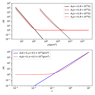
Figure 6: Amplification factors $A_{q}$, $A_{r}$, and $A_{b}$ for the relative error of $\epsilon$, as defined in Eq. (80), for the example of cold matter obeying the MS1 EOS. Top panel: amplification as a function of density, for fixed magnetic field and velocity. Bottom panel: amplification versus velocity, for fixed density and no magnetic field.

V.4 Interaction with recovery corrections

Enforcing the evolved variables to stay in the physically valid regime corresponds to a projection onto the validity boundary. Depending on the choice of projection, it is possible that the corrections cause a drift along the boundary, in the worst case with a preferred direction. This is of particular concern for the very frequent correction of limiting the specific energy above the zero temperature value. For our scheme, only the energy density is corrected in that case. Therefore, it does not introduce a drift of the evolved momentum density.

The main effect of limiting $\epsilon$ above the zero temperature value may be to induce a spurious heating. The reason is that cutting the evolution error distribution from below creates a positive bias until the error distribution has little support below the cut. Of course, the raw error distribution before the correction could already contain a bias. For the idealized case in which the evolution errors follow a zero-mean normal distribution around the correct result, we expect the temperature to increase until the thermal energy reaches a level comparable to the width of the error distribution for total energy.

Note that excessive artificial heating could reduce the velocity, since the momentum density incorporates a factor $h$. However, if $h$ is significantly increased non-homogeneously by the errors, the corresponding changes in thermal pressure can be expected to cause gradients and corresponding acceleration.

In the above discussion, we omitted the effect of finite root solving accuracy. Our implementation of the algorithm recomputes all conserved variables from the primitive ones if, and only if, corrections were required. Therefore, the momentum only remains constant to the accuracy of the root solving when applying the correction to the energy. This error is formally bounded by Eq. (74). We cannot predict, however, if the distribution limited by this bound is symmetric or not. Any bias might lead to a cumulative effect over many corrections. For the worst possible scenario where each correction leads to the maximum possible momentum error always pointing along the momentum, a few thousand corrections could add up to intolerable levels.

To assess the actual behavior, we performed a numerical experiment. Instead of using a full numerical evolution, we employ a random walk model representing an evolution error, starting at selected states. After each “evolution” step, we apply the primitive recovery and limit the conserved variables to the allowed regime. The cumulative corrections applied to energy and momentum are monitored.

In this approach, we can prescribe the error distribution. As a worst case example, we use a normal distribution with negative mean for the energy error. Starting at a zero temperature state, this causes frequent corrections to the energy. Note that the expected error in the momentum does not depend on the magnitude of the corrections, but this randomized test nevertheless involves different magnitudes. For the root finding accuracy, we use four different values $\Delta=10^{-7},10^{-8},10^{-9},10^{-10}$.

We find that the average momentum error is orders of magnitude smaller than the limit Eq. (74). Selecting an initial state $v=0.99,b=2,\rho=6\times 10^{12}\usk\mathrm{g}\mathrm{/}\mathrm{c}\mathrm{m}\mathrm{{}^{3}}$, the momentum errors of individual correction steps approach machine precision levels around $\Delta=10^{-9}$. We believe that the reason might be that the accuracy increases drastically during the final root finding step, such that the average root error is much smaller than the prescribed maximum. We conclude that cumulative effects of the corrections can likely be neglected. In case of evidence to the contrary, the solution would be to simply not recompute the momentum, sacrificing machine-precision consistency for error reduction.

We also apply the random walk model to states with different combinations of $b=\{0,2\}$, $v=\{0,0.99\}$, $\epsilon_{\mathrm{th}}=\{0,10\}$, perturbing the evolved variables separately with normally distributed relative errors of order $10^{-4}$. This test confirms that the implementation of the zero-temperature energy correction works as intended. We monitored the behavior of $v^{i},W,\epsilon,P,\mu$ for the above cases and did not encounter any problematic behavior.

VI Summary and Discussion

In this work, we solved the technical problem of primitive variable recovery in relativistic ideal magnetohydrodynamic evolution codes via a new fully reliable scheme. We derived a mathematical proof that the algorithm always finds a valid solution, and that the solution is unique. Moreover, we derived expressions that allow us to prescribe the accuracy of the individual primitive variables.

The guaranteed reliability of the new algorithm is a big advantage compared to older methods, which are able to handle most of the parameter space encountered in BNS merger scenarios, but may still fail in some cases Siegel et al. (2018). Even rare recovery failures are very problematic, since they necessitate manual intervention, and may require repeating parts of the simulation. Recovery failures are practically unpredictable and potentially chaotic (we recall the Newton-Raphson fractal related to convergence properties of a standard root finding procedure). This is aggravated for recovery schemes that rely on an initial guess taken from the previous timestep. The automated approach of using a fixed state (e.g., artificial atmosphere) in case of recovery failure will render simulations unpredictable in practice.

The ability to identify unphysical evolved variables, as well as the nature of the invalidity, is another advantage of our method. All evolution schemes produce unphysical states occasionally, most of which are harmless. However, sometimes invalid input occurs as the first symptom of more severe evolution errors. Our method allows to prescribe an error policy and selectively apply corrections based on the nature of the problem. Such corrections (or lack of corrections) should be considered as part of the evolution scheme, but they are mentioned in the literature only rarely.

The design of our scheme naturally suggests a particular prescription for correcting slightly unphysical input. We discussed potential cumulative effects of those corrections, and predicted that it will create artificial heating if the matter is close to zero temperature. We also showed that there should be no direct impact on the momentum. We validated this by performing a numerical experiment using random walk perturbations to emulate evolution errors.

Since the implementation of recovery algorithms is a work-intensive endeavor, we are making our reference implementation public in form of a well-documented library named RePrimAnd Kastaun (2020), which can be used by any evolution code. In order to be useful in practice, the recovery should not constrain the type of EOS. Therefore, our recovery algorithm is formulated in an EOS-agnostic manner, and the reference implementation contains a generic interface for using arbitrary EOS.

We subjected the code to a comprehensive suite of tests, demonstrating that both the algorithm and the actual implementation are robust up to Lorentz factors and values of magnetization much larger than those relevant for BNS mergers. We also showed that the scheme is computationally efficient regarding the number of EOS evaluations (efficiency of EOS implementations aside).

While investigating the accuracy of the recovery scheme, we identified regimes where rounding errors are amplified by unavoidable cancellation errors. We quantified the dominant contributions and found that the accuracy measured in our tests is compatible with the predictions. We also found that the rounding errors are irrelevant because the very same cancellation also leads to the amplification of evolution errors. Investigating the error propagation from evolved to primitive variables, we showed that the accuracy of the thermal energy and thermal pressure can severely degrade when evolving strongly magnetized regions of low density.

We believe that our results will be useful in particular for studying the launching mechanism of jets powering SGRBs, as well as the mass ejection processes that are ultimately responsible for kilonova signals. Both astrophysical scenarios involve strongly magnetized matter.

Appendix A Derivations

In this appendix, we provide derivation steps left out in the main text. First, we derive Eq. (65) for the derivative of the master function. Starting from Eq. (44),

$$f =\mu-\hat{\mu}=\mu-\left(\hat{\nu}+\mathrm{bar}{r}^{2}\mu\right)^{-1}\,,$$ (83)

$$f^{\prime} =1+\left(\hat{\nu}+\mathrm{bar}{r}^{2}\mu\right)^{-2}\left(\hat{\nu}^{\prime}+\mathrm{bar}{r}^{2}+2\mathrm{bar}{r}\mathrm{bar}{r}^{\prime}\mu\right)\,,$$ (84)

$$=1+\hat{\mu}^{2}\left(\hat{\nu}^{\prime}+\mathrm{bar}{r}^{2}-2\left(1-x\right)x^{2}r_{\bot}^{2}\right)\,,$$ (85)

where primes denote derivatives with respect to $\mu$. We first consider the case where $\epsilon$ computed from Eq. (42) does not exceed the upper limit allowed by the EOS (but may be smaller than the zero temperature limit). For those cases, we can use Eq. (64) to get

$$\begin{split}f^{\prime}&=1+\hat{\mu}^{2}\Biggl{(}-\left(1+c_{s}^{2}\right)\hat{\nu}\frac{\hat{W}^{\prime}}{\hat{W}}\\ &\qquad\qquad\quad+\mathrm{bar}{r}^{2}-2\left(1-x\right)x^{2}r_{\bot}^{2}\Biggr{)}\end{split}$$ (86)

$$\begin{split}&=1+\hat{\mu}^{2}\Biggl{(}-\left(1+c_{s}^{2}\right)\hat{\nu}\hat{W}^{2}\mu\left(x^{3}r_{\bot}^{2}+r_{\|}^{2}\right)\\ &\qquad\qquad\quad+x^{2}r_{\bot}^{2}+r_{\|}^{2}-2\left(1-x\right)x^{2}r_{\bot}^{2}\Biggr{)}\end{split}$$ (87)

At a solution, we have $\hat{\mu}=\mu$ and $\hat{\nu}\hat{W}^{2}\mu=1$, which leads to

$$\begin{split}f^{\prime}&=1+\mu^{2}\Biggl{(}-\left(1+c_{s}^{2}\right)\left(x^{3}r_{\bot}^{2}+r_{\|}^{2}\right)\\ &\qquad\qquad\quad+x^{2}r_{\bot}^{2}+r_{\|}^{2}-2\left(1-x\right)x^{2}r_{\bot}^{2}\Biggr{)}\end{split}$$ (88)

$$=1+\mu^{2}\left(\left(1-c_{s}^{2}\right)\left(x^{3}r_{\bot}^{2}+r_{\|}^{2}\right)-x^{2}r_{\bot}^{2}-r_{\|}^{2}\right)$$ (89)

$$=1-\mu^{2}\mathrm{bar}{r}^{2}+\mu^{2}\left(1-c_{s}^{2}\right)\left(x^{3}r_{\bot}^{2}+r_{\|}^{2}\right)$$ (90)

Using that $\hat{v}=\mu\mathrm{bar}{r}$ at the solution, we arrive at Eq. (65).

We now address the case where $\epsilon$ computed from Eq. (42) does exceed the limit $\epsilon_{\mathrm{max}}$ below which the EOS is valid. Eq. (48) then becomes

$$\hat{\nu} =\nu_{B}=\left(1+\hat{a}\right)\left(1+\mathrm{bar}{q}-\mu\mathrm{bar}{r}^{2}\right)$$ (91)

$$\hat{\nu}^{\prime} =\frac{\hat{\nu}}{1+\hat{a}}\hat{a}^{\prime}+\left(1+\hat{a}\right)\left(\mathrm{bar}{q}^{\prime}-\mathrm{bar}{r}^{2}-2\mu\mathrm{bar}{r}\mathrm{bar}{r}^{\prime}\right)$$ (92)

Inserting Eq. (56), Eq. (57), and Eq. (30) yields

$$\frac{\hat{\nu}^{\prime}}{\hat{\nu}} =\frac{\hat{a}^{\prime}}{1+\hat{a}}-\frac{1+\hat{a}}{\hat{\nu}}R^{2}$$ (93)

with $R^{2}\equiv x^{3}r_{\bot}^{2}+r_{\|}^{2}\leq\mathrm{bar}{r}^{2}$. For the case at hand, ${\hat{a}(\hat{\rho})=a(\hat{\rho},\epsilon_{\mathrm{max}}(\hat{\rho}))}$, and hence

$$\hat{a}^{\prime} =\hat{\rho}^{\prime}\left(\frac{\partial a}{\partial\rho}+\frac{\mathrm{d}\epsilon_{\mathrm{max}}}{\mathrm{d}\rho}\frac{\partial a}{\partial\epsilon}\right)$$ (94)

Splitting the derivative of $\epsilon_{\mathrm{max}}$ into adiabatic and residual contributions by using definition Eq. (67), we obtain

$$\hat{a}^{\prime} =\hat{\rho}^{\prime}\left(\frac{\partial a}{\partial\rho}+\left(\frac{\hat{P}}{\hat{\rho}^{2}}+\frac{A(\hat{\rho})}{\hat{\rho}}\right)\frac{\partial a}{\partial\epsilon}\right)$$ (95)

$$=\hat{\rho}^{\prime}\left(\left.\frac{\mathrm{d}a}{\mathrm{d}\rho}\right|_{s}+\frac{A(\hat{\rho})}{\hat{\rho}}\frac{\partial a}{\partial\epsilon}\right)$$ (96)

One can express the adiabatic soundspeed in terms of $a$ as

$$\left.\frac{\mathrm{d}a}{\mathrm{d}\rho}\right|_{s} =\frac{1+a}{\rho}\left(c_{s}^{2}-a\right)$$ (97)

which allows us to write

$$\hat{a}^{\prime} =\frac{\hat{\rho}^{\prime}}{\hat{\rho}}\left(\left(1+\hat{a}\right)\left(c_{s}^{2}-\hat{a}\right)+A\frac{\partial a}{\partial\epsilon}\right)$$ (98)

Evaluating at the solution, we can use $\hat{\mu}=\mu$ and $\hat{W}^{2}\hat{\nu}\mu=1$. Using also Eq. (59) and Eq. (60), we get

$$\frac{\hat{\nu}^{\prime}}{\hat{\nu}} =-\hat{W}^{2}\mu R^{2}\left(1+c_{s}^{2}+\frac{A}{1+\hat{a}}\frac{\partial a}{\partial\epsilon}\right)$$ (99)

Inserting into Eq. (85), we can rewrite the master function derivative at the solution as

$$f^{\prime} =1-\hat{v}^{2}+\hat{v}^{2}\frac{R^{2}}{\mathrm{bar}{r}^{2}}\left(1-c_{s}^{2}-\frac{A}{1+\hat{a}}\frac{\partial a}{\partial\epsilon}\right)$$ (100)

If Eq. (66) holds, $f^{\prime}$ is always strictly positive at the solution, as claimed in Sec. II.7.

Finally, we need to discuss the corner case where the mass density computed in Eq. (41) is outside the valid range of the EOS. If $\mathrm{bar}{D}/\hat{W}(\mu_{+})>\rho_{\mathrm{max}}$ or $\mathrm{bar}{D}<\rho_{\mathrm{min}}$, there is no solution with valid density and no need to determine the root. The only complication arises when $\mathrm{bar}{D}/\hat{W}(\mu_{+})<\rho_{\mathrm{max}}<\mathrm{bar}{D}$ or $\mathrm{bar}{D}/\hat{W}(\mu_{+})<\rho_{\mathrm{min}}<\mathrm{bar}{D}$. Although the proof for the existence of a solution remains valid in those cases, we did not succeed to prove uniqueness of the master function root on the range $(0,\mu_{+}]$. Luckily, it is not necessary to prove uniqueness on the full interval. Instead, we numerically solve $\mathrm{bar}{D}/\hat{W}(\mu)=\rho_{\mathrm{min/max}}$ for $\mu$. We recall that $\hat{W}(\mu)$ is an analytic expression that does not involve the EOS, and monotonically increases with $\mu$. Hence we can find a sub-interval $(\mu_{a},\mu_{b})\subseteq(0,\mu_{+})$ that consists of all values for which the density $\mathrm{bar}{D}/\hat{W}(\mu)$ is valid. We already know that the master function $f$ has at most one root on that interval. There is a solution with valid density if and only if $f(\mu_{a})$ and $f(\mu_{b})$ have opposite sign, which is easy to check. Using an initial bracket $(\mu_{a},\mu_{b})$ for the root finding then ensures uniqueness.