Sterile Neutrinos and the Global Reactor Antineutrino Dataset
Abstract
We present results from global fits to the available reactor antineutrino dataset, as of Fall 2019, to determine the global preference for a fourth, sterile neutrino. We have separately considered experiments that measure the integrated inverse-beta decay (IBD) rate from those that measure the energy spectrum of IBD events at one or more locations. The software used is the newly developed GLoBESfit tool set which is based on the publicly available GLoBES framework and will be released as open-source software.
I Introduction
Nuclear reactors have been workhorses for neutrino physics since its inception as an experimental science by Cowan and Reines Cowan et al. (1956). A number of important measurements of fundamental neutrino111We consider “neutrino” to be synonymous with “electron antineutrino” in this work. properties have been made using reactor neutrinos: we highlight the confirmation of solar neutrino flavor conversion by KamLAND Eguchi et al. (2003) and the measurement of An et al. (2012); Ahn et al. (2012); Abe et al. (2012). Neutrinos are not produced in the fission process itself but in the subsequent beta decays of neutron-rich fission fragments. The first reactor neutrino experiments already had to deal with the question of how to predict the neutrino flux from these complex sources Carter et al. (1959a); interestingly, the uncertainty quoted was 5-10%. The neutrino flux question has taken on a central role with reactor antineutrino anomaly (RAA) Mention et al. (2011): an initial reactor flux re-evaluation Mueller et al. (2011), later confirmed by one of the present authors Huber (2011), lead to an increase in predicted reactor neutrino event rates and thus to an observed deficit of reactor neutrinos.
An exciting, albeit speculative, explanation would be provided by oscillations into a sterile neutrino with . Unsurprisingly, this hypothesis has triggered significant interest Abazajian et al. (2012), resulting in a number of new reactor neutrino experiments aimed at finding an actual oscillation signature. At the same time, this interest also resulted in a significant effort, both theoretically and experimentally, to improve reactor neutrino flux predictions; see, for instance, Ref. Hayes and Vogel (2016) and references therein.
The interpretation of reactor neutrino data in terms of sterile neutrino oscillations is relatively straightforward and free of major tension, even when combined with other available electron neutrino disappearance data; see, e.g., Ref. Dentler et al. (2018); Gariazzo et al. (2017). However, when an attempt is made to explain also the anomalous results in the and channels as observed by LSND Aguilar-Arevalo et al. (2001) and MiniBooNE Aguilar-Arevalo et al. (2013) significant tension arises: for a sterile neutrino to be able to mediate the transition between two different active flavors, the sterile neutrino must mix with both of these flavors. As a result, there is a well-defined relationship between the amplitude of oscillations and the expected effect in the disappearance channels and . The size of the RAA is consistent with sterile neutrino interpretation of LSND and MiniBooNE, but no evidence is found for commensurate disappearance in the channel. This issue has persisted for some time and there is debate about the statistical significance of this tension, for a recent review see Ref. Diaz et al. (2019). Nonetheless, the lack of disappearance presents a considerable deficiency in the sterile neutrino hypothesis. Here, we remain agnostic with respect to LSND and MiniBooNE and focus entirely on the electron neutrino sector.
Given the significant ongoing experimental effort in reactor neutrino experiments, combined with the potential for a major discovery of new physics, we will discuss in detail the existing reactor antineutrino data. We will compare the data with the Huber-Mueller flux model, as well as with two state-of-the-art flux predictions, one based on the summation approach Estienne et al. (2019) and one based on the conversion approach Hayen et al. (2019). We will critically examine how these differing flux models affect the evidence for the sterile neutrino hypothesis. Moreover, we present an open-source software framework called GLoBESfit based on the established GLoBES Huber et al. (2005, 2007) software suite, which will allow users to fit their preferred model to the data. We also hope that this open framework can be adopted by the experimental community to share their results.
A major result of this work is that we find if we restrict the analysis to data taken after 2010 – i.e., the modern reactor experiments and their short-baseline counterparts – then the reactor rate anomaly seems to be enhanced. This restriction should not be misconstrued as a lack of trust in the older experiments, but it does reflect the fact that data curation and release practices were less refined in the past. As a result, much less detailed information is available for properly including older experiments into a global fit.
Best practices in data sharing are crucial for this field to make progress, since we have previously shown Berryman and Huber (2019) that no single, existing reactor experiment can definitively test the currently preferred parameter space. Therefore, global fits will play an important role in neutrino physics for the foreseeable future, reinforcing the value of an open fitting framework.
This manuscript is arranged as follows. In Sec. II, we discuss the predictions of the fluxes of antineutrinos at nuclear reactors that we use, including how systematic uncertainties on these predictions are incorporated in our analyses. In Sec. III, we discuss the total IBD rate experiments that we have included in our fits, and in Sec. IV, we present our combined analyses of various subsets of these data. Similarly, in Sec. V, we discuss the IBD spectrum experiments that we have included in our analyses, and in Sec. VI we present combined analyses of these experiments. We address the effect of the infamous 5 MeV bump Choi et al. (2016); An et al. (2016); Abe et al. (2016) on sterile neutrino searches in Sec. VII, and offer concluding remarks in Sec. IX.
In addition to communicating our findings, one of the intentions of this manuscript is to provide documentation for the tools that we have developed. Pursuant to this, we have included several appendices that deal with technical aspects of GLoBESfit. In Appendix A, we provide an account of how oscillations involving a sterile neutrino have been included in GLoBES, and in Appendix B, we provide a general overview of the files that constitute GLoBESfit, including their content and some aspects of their functionality. Lastly, we provide extensive data tables and supplemental figures in Appendix C; these data are important for our analyses, but would have been intrusive to have included in the main text.
II Reactor Antineutrino Flux Models
Predictions of the spectra of antineutrinos from reactors have played a central role from the inception of neutrino physics as experimental science Carter et al. (1959b). More recently, the RAA Mention et al. (2011) has put a spotlight on flux models; for a recent review on flux models and how they are produced, see Ref. Hayes and Vogel (2016). For the discussion here, we note the following the salient features. Neutrinos are produced not by the fission process itself, but by the beta decays of about 800 fission fragment isotopes, corresponding to about 10,000 beta decay branches. A large fraction of these beta decays are of (unique and non-unique) forbidden type, which implies a significant dependence on details of nuclear structure for both the emitted electron and antineutrino spectra. We will use the following three flux models:
-
1.
Huber-Mueller (HM): This flux model Mueller et al. (2011); Huber (2011) has become the de facto standard in the field and is based on the conversion of integrated beta spectrum measurements performed in the 1980s at the Institut Laue-Langevin Von Feilitzsch et al. (1982); Schreckenbach et al. (1985); Hahn et al. (1989). This flux model has relatively little dependence on nuclear databases and employs the allowed approximation, i.e., all beta decays are treated as allowed decays.
-
2.
Ab initio: This flux model Estienne et al. (2019) uses fission fragment yields and information on individual beta decays from nuclear databases to directly compute the neutrino flux. It also employs the allowed approximation.
-
3.
Hayen-Kostensalo-Severijns-Suhonen (HKSS): This flux model Hayen et al. (2019) shares many of the features of HM, that is, it is based on a conversion of the integrated beta spectra. Importantly, it is the first attempt to include effects from forbidden decays in a systematic fashion.
The ratios for the ab initio and HKSS flux predictions relative to the HM predictions are shown in Figs. 1(a)-1(d) for, respectively, 235U, 238U, 239Pu and 241Pu. In each panel, the orange line at represents the HM predictions; the blue curve represents the ab initio predictions; and the dark cyan curves represent the HKSS predictions. The associated bands represent the () systematic uncertainties on these predictions; we discuss how these are calculated below. For comparison, we also show the measured neutrino spectrum from Daya Bay Adey et al. (2019a) (red) and PROSPECT Ashenfelter et al. (2019) (pink). Daya Bay can separate the contributions from 235U and 239Pu by comparing data taken at different points in the fuel cycle. Meanwhile, PROSPECT is deployed at HFIR, which is fueled with highly-enriched uranium meaning nearly all fissions are of 235U. Visual inspection indicates that all three flux models and the neutrino data agree for 239Pu within the large error bars. However, the ab initio flux model predicts a lower flux for 235U than either HM or HKSS, which seems to agree somewhat better with data. Comparison of the data with any of three flux models reveals a bump in the region around 5-6 MeV. In later sections, we will perform a more careful analysis; impressions from this intial inspection will essentially be confirmed.
In all these calculations, one should formally be accounting for nonequilibrium corrections to the antineutrino flux; these are approximated by Mueller, et al., in Ref. Mueller et al. (2011) for 235U, 239Pu and 241Pu. However, the collaborations often do not publish information about their burn-up, so it is unclear how large the nonequilibrium correction should be. Even taking a nonequilibrium correction corresponding to 450 days of irradiation – the largest such correction presented in Ref. Mueller et al. (2011) – the difference between this the absence of nonequilibrium correction is typically overwhelmed by both experimental and other theoretical uncertainties. Therefore, we do not expect these to meaningfully impact the final results; we therefore elect to exclude them from the present analyses.
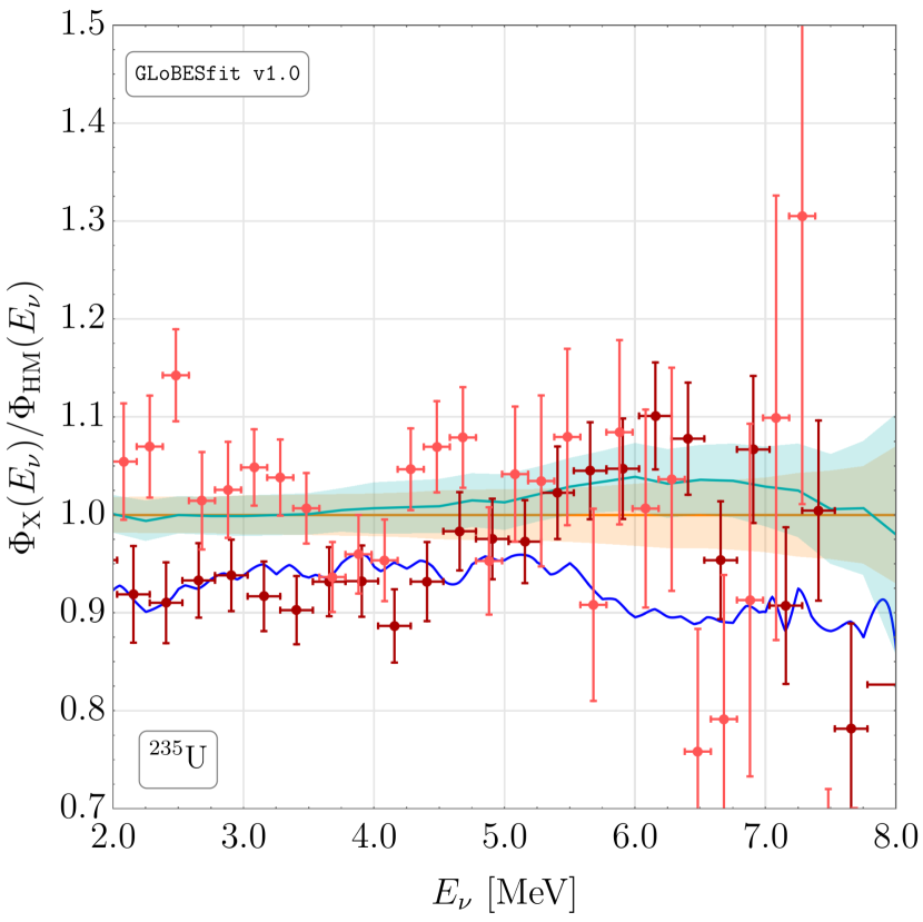
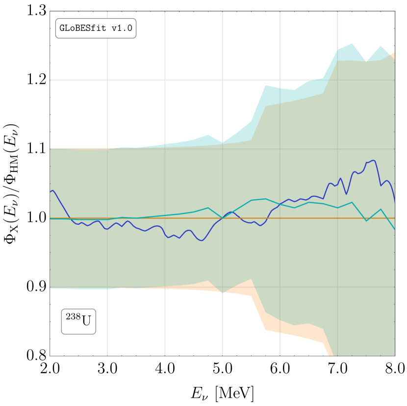
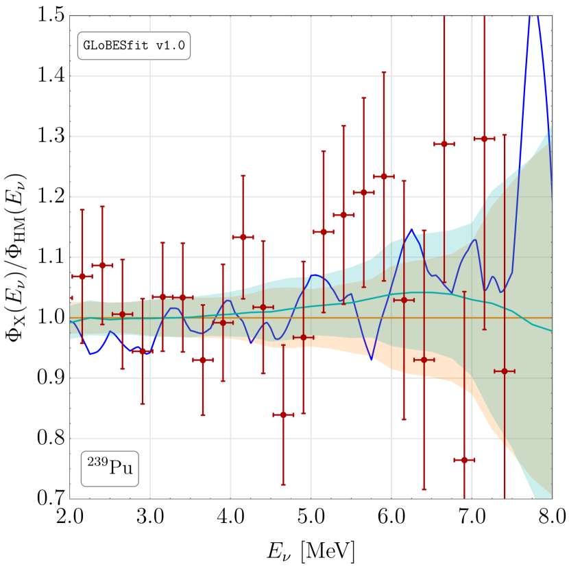
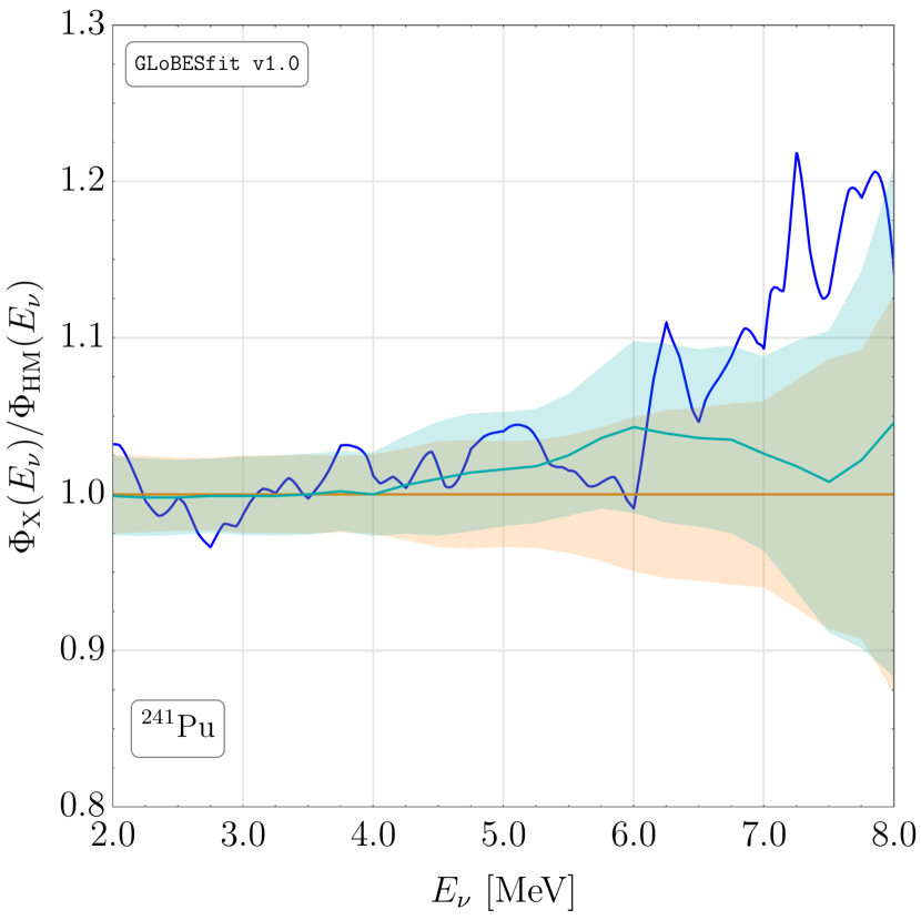
The experimental quantity of interest in all cases is the convolution of the neutrino flux with the inverse beta decay (IBD) cross section and the electron-type survival probability (see Eq. (A.7) in Appendix A). We define the flux weighted cross sections as follows:
| (II.1) |
This quantity provides the IBD rate for antineutrinos with true energy in the range calculated using flux model X = HM, AI, HKSS for isotope . The total IBD rate in this energy window is then the sum of the , weighted by the appropriate effective fuel fraction , i.e., the fraction of fissions due to each isotope during the operation of the experiment. In this work, we use the IBD cross section published in Ref. Vogel and Beacom (1999) – particularly, the results up to and including as given in their Eqs. (14) and (15). The uncertainty on this cross section is negligible compared to the uncertainties on the fluxes.
We consider two types of reactor antineutrino measurements in this work. In Secs. III and IV, we consider experiments that measure the total IBD rate, but not necessarily the specific energy of a given event. For these, we will take MeV. On the other hand, in Secs. V and VI, we consider measurements of the IBD spectrum over various energy bins, each with its own . Our treatment of the flux systematics at total IBD rate experiments is common to all such experiments; the flux systematics at spectrum experiments must be handled on a case-by-case basis.
We use the following generic procedure to incorporate systematic uncertainties stemming from flux predictions into our analyses.
-
1.
We use information presented in the literature to assign a covariance matrix to a set of flux predictions.
-
2.
We then generate random variations of these fluxes using this covariance matrix to numerically calculate in Eq. (II.1), assuming , for some specified .
-
3.
For total rate analyses, we take MeV and calculate the and their correlations. These results will be applied to all total IBD rate measurements simultaneously, as will be described in Sec. IV.
- 4.
When we numerically integrate over the predicted fluxes, we do so by logarithmically interpolating/extrapolating on the published flux models.
HM Fluxes
For the HM fluxes we use the central values published in Tables VII-IX of Ref. Huber (2011) for the fluxes from 235U, 239Pu and 241Pu, respectively, whereas we use the values from the “, 12 h” column of Table III of Ref. Mueller et al. (2011) for 238U. Regarding errors, we use the following prescription. For 235U, 239Pu and 241Pu, we take the (percent) errors listed in the columns headed “stat.” and “bias err.” from Tables VII-IX of Ref. Huber (2011), respectively, to be fully uncorrelated between bins and these three isotopes; and the columns headed “,” “WM” and “norm.” are added in quadrature and taken to be fully correlated between bins and these three isotopes. We assume all errors to be Gaussian; asymmetric errors are replaced by a Gaussian with width given by the geometric mean of the upper and lower uncertainties. For 238U, we combine the errors in the “Nuclear databases” column of Table II in Ref. Mueller et al. (2011)– the correlations of which are shown in Table I of the same reference – along with the “Missing info.” column of the same – which we take to be fully correlated. These uncertainties yield the orange bands in Figs. 1(a)-1(d).
With the information described above, we obtain the following IBD yields for the HM fluxes:
The uncertainties on the HM fluxes are described by the following correlation matrix:
| (II.2) |
the ordering here is {235U, 238U, 239Pu, 241Pu}. We reiterate that we are ignoring uncertainties from the IBD cross section; the dominant theoretical uncertainty is that on the antineutrino flux.
Ab Initio Fluxes
The values of the antineutrino fluxes can be found in the Supplementary Material to Ref. Estienne et al. (2019).222We thank Muriel Fallot for providing us with these fluxes in machine readable format Fallot . These predictions, however, are not published with systematic uncertainties; consequently, we show no blue shaded regions in Figs. 1(a)-1(d).
In our analyses, we will always apply the systematic errors associated to the HM fluxes to the ab initio fluxes, as well. This is likely an optimistic assignment; though precise uncertainties have not been calculated, the true systematic uncertainty on these predictions is likely of order . However, we will argue below that this treatment is sufficient for the conclusions of this work. For now, we simply point out that this treatment results in a more aggressive assignment of statistical significances than a more realistic error budget would produce.
We calculate the following isotopic IBD yields:
While the isotopic fluxes for 238U, 239Pu and 241Pu here are consistent with those calculated for the HM fluxes, the 235U flux is substantially lessened. This is apparent from Fig. 1(a): the ab initio 235U flux is about less than the corresponding HM prediction for most energies. The corresponding correlation matrix is given by
| (II.3) |
HKSS Fluxes
The fluxes are presented in Tables VI-IX of Ref. Hayen et al. (2019); specifically, we use the results in the columns headed “ Num.,” which represent the (percent) rescaling introduced by including first-forbidden decays to the reactor antineutrino flux. Systematics are handled by splicing together a subset of the errors published in Ref. Hayen et al. (2019) with those for the HM fluxes from Ref. Mueller et al. (2011); Huber (2011). Specifically, we use all the components of the HM uncertainty budget discussed above, and we add to this the uncertainties under the columns headed “” and “Param.” in Tables VI-IX of Ref. Hayen et al. (2019); these latter components are each taken to be totally correlated between bins and isotopes. These uncertainties yield the dark cyan bands in Figs. 1(a)-1(d).
The procedure outlined above gives us the following isotopic IBD yields:
Note that these have increased by relative to the nominal HM predictions. The uncertainties have also grown, stemming from uncertainty related to and the parametrization procedure used in Ref. Hayen et al. (2019), but the change is quite modest — including first-forbidden contributions has not resulted in a grossly inflated error budget. These results are described by the following correlation matrix:
| (II.4) |
Unlike for the HM and ab initio flux predictions, the flux from 238U is now correlated with the three other isotopes via the axial coupling .
III Rate Experiments
In this section, we describe the experiments that have measured the IBD rate that enter into our analysis and how these are defined in GLoBES. We are ultimately interested in the ratio of the measured IBD rate relative to one of (1) the HM predictions, (2) the ab initio predictions, or (3) the HKSS predictions. These are compared against the experimentally determined ratios relative to the same flux prediction. Many of the details regarding specific implementations of these experiments are the same between them; we relegate discussion of these to Appendix B.
III.1 Short-Baseline Experiments
Bugey-4
The detector width is taken to be 3.0 m and the core is assumed to be point-like. The center-to-center distance between the core and the detector is 15 m. The fuel fractions published by the collaboration Declais et al. (1994) are
The experimental resolution is not published by the collaboration. In the absence of further input, we take the resolution to be , which is the stated resolution for Bugey-3. The published total IBD yield is cm2/fission Declais et al. (1994); this leads us to , and . Following Refs. Giunti (2017); Gariazzo et al. (2017), the experimental uncertainty is taken to be , which is entirely correlated with Rovno 91.
Rovno 91
Rovno 91 used the same detector as Bugey-4; the baseline, however, is different – namely, 18 m. The fuel fractions published by the collaboration Kuvshinnikov et al. (1991) are333Refs. Giunti (2017); Gariazzo et al. (2017) use the following values in their analyses: We use the values from the collaboration, instead.
The resolution is not published by the collaboration. In the absence of further input, we take the resolution to be , as for Bugey-4. The absolute IBD cross section measured at Rovno 91 is cm2/fission Kuvshinnikov et al. (1991). We find , and . The total experimental uncertainty is , of which is correlated with Bugey-4.
Bugey-3
The collaboration reports IBD rate measurements at 15 m, 40 m and 95 m. The fuel fractions published by the collaboration Declais et al. (1995) are:
which we assume applies to all three measurements. The collaboration claims an energy resolution of .
The collaboration only publishes the ratios of their measurements with respect to Refs. Schreckenbach et al. (1985); Hahn et al. (1989); we instead derive IBD cross sections from their stated event rates and experimental specifics and find cm2/fission. We find , ; and . The total uncertainties are, respectively, {4.2%, 4.3%, 15.2%}, of which 4.0% is correlated between each of these three experiments.
Gösgen
IBD rate measurements are reported Zacek et al. (1986) at 37.9 m, 45.9 m and 64.7 m; the detector is taken to be 2.0 m wide, while the core is taken to be point-like. The effective fuel fractions for the three measurements are slightly different:
The collaboration claims an energy resolution .
From Ref. Zacek et al. (1986), we derive cm2/fission. This leads us to ; ; and . The total uncertainties are, respectively, {5.4%, 5.4%, 6.7%}, of which 2.0% is correlated between each of these three experiments; there exists an additional 3.8% correlation between each of these and the ILL experiment.
ILL
We mostly follow Ref. Kwon et al. (1981); however, we also correct for the fact that Ref. Hoummada et al. (1995) reports that the original power of the ILL experiment was underreported by 9.5%. The detector width is 2.0 m, the core is assumed to be point-like and the center-to-center distance is 8.76 m. The core consists of 93% enriched 235U; our analysis assumes that this is the only relevant isotope. The energy resolution is taken to be .
We determine from Refs. Kwon et al. (1981); Hoummada et al. (1995) that cm2/fission, implying the ratios , and . The experimental uncertainty is 9.1%, of which 3.8% is correlated with each of the three Gösgen measurements.
Krasnoyarsk 87
The detector is taken to have a width of 2.0 m while the core is point-like and comprised purely of 235U. The center-to-center distances at these experiments are 32.8 m and 92.3 m. The energy resolution is not specified in Ref. Vidyakin et al. (1987); we assume it to be . The collaboration explicitly publishes IBD yields for the two experiments: cm2/fission for {33 m, 92 m}. We calculate , and . The respective errors are {5.0%, 20.4%}, of which 4.1% is fully correlated between these experiments.
Krasnoyarsk 94
We essentially repeat the analysis of Krasnoyarsk 87, except that the center-to-center distance is now taken to be 57.0 m. As before, the reactor is approximated to be purely 235U and the energy resolution is . The collaboration publishes the IBD yield as cm2/fission Vidyakin et al. (1994); this results in , and . The uncertainty is 4.2% and is uncorrelated with any other experiment.
Krasnoyarsk 99
We again re-use the Krasnoyarsk analysis with a center-to-center distance of 34.0 m and a core of pure 235U. The energy resolution is again taken to be . The collaboration publishes the IBD yield as cm2/fission Kozlov et al. (2000); this yields , and . The corresponding uncertainty is 3.0%, which is uncorrelated with any other experiment.
Ref. Kozlov et al. (2000) also includes measurements of charged- and neutral-current deuterium disintegration rates, but these are significantly less precise than the IBD rate measurement; we do not include these in our fits.
Savannah River
The detector is taken to have a width of 2.0 m and the center-to-center distances are 18.2 m and 23.8 m in the two detector configurations with a core of essentially pure 235U. The energy resolution is taken to be . The collaboration does not explicitly report their inferred IBD rate, but from the integrated rates in Table III of Ref. Greenwood et al. (1996) and other experimental information, we derive cm2/fission. These imply ; ; and . The respective uncertainties are {2.8%, 2.9%}, which are each uncorrelated with any other experiment, including each other.
Rovno 88
There are five measurements under the Rovno 88 umbrella Afonin et al. (1988). The first two (1I and 2I) are polyethylene detectors studded with 3He proportional counters, each located 18 m from the core. The latter three (1S, 2S and 3S) are liquid scintillation detectors; 1S and 3S are located 18 m from the core, while 2S is located 25 m from the core.444The 18 m experiments all formally have slightly different baselines — this can be seen clearly in the values of in Table II of Ref. Afonin et al. (1988). However, we expect these differences to be small, so we ignore them. Each detector has a width of 1.0 m, which is roughly consistent with Fig. 1 of Ref. Afonin et al. (1988), and the resolution is taken to be .
Each measurements takes different effective fuel fractions:
In Table III of Ref. Afonin et al. (1988), the collaboration has provided their inferred IBD rate for each of these five experiments. However, in Table II of the same reference, they provide various experimental data that can, in principle, be used to rederive their results. Using the information in that table, Eq. (8) and the updated energies per fission Kopeikin (2012), we derive cm2/fission. From this, we calculate
where the order here is {1I, 2I, 1S, 2S, 3S}. The respective errors are {6.4%, 6.4%, 7.3%, 7.3%, 6.8%}; there exists a 3.1% correlated error between 1I and 2I, as well as between each of 1S, 2S and 3S; moreover, there exists a further 2.2% correlation between either of 1I and 2I and any of 1S, 2S and 3S.
Nucifer
Given the short distance between the core and detector (7.21 m), one might worry that the finite extent of both the reactor core and of the detector may be important in determining the correct oscillation probabilities. However, given that Nucifer reports a total rate measurement, and given the relatively poor energy resolution, we find that this effect is not quantitatively important here.
The composition of the core is Boireau et al. (2016)
The core is dominated by 235U, but since the effective fuel fractions for all four isotopes have been provided, we take these into account. The collaboration claims an energy resolution of . From their reported event rate and other experimental specifics, we estimate the IBD rate to be cm2/fission. This leads to , and . The experimental uncertainty is 10.7% and is uncorrelated with any other experiment.
III.2 Medium-Baseline Experiments – Total Rates
We now turn our attention to medium-baseline oscillation experiments. At these distances, m, two-flavor oscillations are insufficient; we must at least account for nonzero and (or the effective mass splitting ). In practice, we include full four-neutrino oscillations, though we keep the relevant parameters from three-neutrino oscillations fixed at their best-fit values from Ref. Esteban et al. (2019):
Note that does not factor into this analysis.
We define each detector width to be 4.0 m and take the reactors to be point-like; this helps high-frequency oscillations to average out smoothly, but otherwise does not impact our analysis. Since medium-baseline experiments are sourced by multiple reactors, our GLoBES definitions must account for the relative contributions of the reactors.
As mentioned, three-neutrino effects are important at these baselines; this can cause some ambiguity in the definition of the ratio . In this work, we always assume that is defined with respect to the absence of oscillations. We contrast this with the expected deficit within the three-neutrino framework relative to the absence of oscillations, which we will call .
Palo Verde
Palo Verde Boehm et al. (2001) consists of three reactor cores; one is located 750 m from the detector and the other two are at 890 m. Table I of Ref. Boehm et al. (2001) presents the operating cycle over the course of the experiment. Assuming the total power of 11.63 GWth is split evenly among the three reactors over the duration of the experiment and accounting for efficiency, the total exposure from the 750 m reactor is 372.6 GWyr, whereas the total exposure from both 890 m reactors is 706.0 GWyr. The fuel fractions are not stated in Ref. Boehm et al. (2001), so we take them from Refs. Giunti (2017); Gariazzo et al. (2017):
The resolution is also not stated in Ref. Boehm et al. (2001), so we assume it to be .
We use information in Ref. Boehm et al. (2001), along with the total proton number in Ref. Miller (2001),555We thank Giorgio Gratta for pointing us to this reference Gratta . to determine cm2/fission. From this, we calculate , and . The uncertainty is taken to be 5.4%, which is uncorrelated with any other experiment. For context, Ref. Zhang et al. (2013) reports a three-neutrino expectation of .
Double Chooz
Double Chooz Abe et al. (2014); De Kerret et al. (2019) consists of two reactors and two detectors; this measurement pertains to the near detector, from which the two reactors are 355 m and 469 m away. We assume that each reactor operates for the same amount of time over the course of the experiment, and that the average powers delivered during those times are the same. The effective fuel fractions are assumed to be the same for each reactor:
We take the energy resolution to be Abe et al. (2014).
Ref. De Kerret et al. (2019) reports cm2/fission. However, this result has been corrected for the effects of nonzero . We calculate , and . The corresponding uncertainty is 1.4%, which is uncorrelated with any other experiment.
Chooz
Chooz Apollonio et al. (2003) consists of two reactors located 998 m and 1115 m away from the detector. The two reactors have different run times and effective powers; the operation periods are broken down in Table 1 of Ref. Apollonio et al. (2003). We assume that the reactors operate at the same average power during the period in which both are operational; this implies that reactor 1 (1115 m) delivered 12715.5 GWh over the experiment, while reactor 2 (998 m) delivered 8556.5 GWh. The effective fuel fractions are assumed to be the same for each reactor:
We take the energy resolution to be 0.5 MeV; Ref. Apollonio et al. (2003) claims a resolution of 0.33 MeV, but we use the more conservative estimate here.
III.3 Medium-Baseline Experiments – Rate Evolution
Daya Bay
The details about the experimental geometry are well documented in Refs. An et al. (2017a, b). We tabulate relevant experimental specifics in Tables 13-17 in Appendix C. The fuel evolution result that we use corresponds to the 1230-day data release; an analogous analysis for the 1958-day data appeared in Ref. Adey et al. (2019a), which we look forward to including in the future.
AD8 did not operate for as long as AD1-3 in the 1230-day dataset; this is characterized by the exposure for detector , defined as
| (III.1) |
where represents the average power of reactor during either the 6AD or 8AD period, and is the operating time of the detector during these periods. The powers are presented in Table 14. For all detectors, days; for ADs 1-3, days, but AD8 has days. Moreover, we account for the different total AD target masses and efficiencies, given in Table 15.
The Daya Bay data are presented in bins of differing fuel fractions. We present the average fuel fractions of these bins and the corresponding IBD rate measurements in Table 16. These IBD rates have been inferred by the collaboration accounting for three-flavor oscillations. To construct our analyses, we correct these measurements by reinserting these effects, assuming the best-fit values presented in Ref. An et al. (2017b):
Our calculations of the ratios , and are also shown in Table 16. Our analyses employ the covariance matrices provided by the collaboration in the Supplementary Material to Ref. An et al. (2017c), appropriately converted from absolute IBD rate to ratio with respect to our IBD predictions. Ref. Adey et al. (2019b) presents a total IBD rate measurement whose systematic uncertainty has been decreased by 29% relative to prior measurements. Following the prescription of Ref. Giunti et al. (2019a), we have decreased the systematic uncertainties from Ref. An et al. (2017c) in our analyses by this amount.
RENO
In Table 18, we show the distances between each RENO reactor and the near and far detectors; in Table 19, we show the average power of each reactor during the experiment;666We thank Soo-Bong Kim for providing this information Kim . and in Table 20, we show other important experimental information, including the detector operating time and efficiency. These data will also be used in the RENO spectral analysis; here, we only need the information for the near detector.
We take the flux-weighted average baseline to be 433.1 m. Out definition of “average baseline” is different from that of RENO Bak et al. (2019); we weight by the reactor flux at the detector, but RENO considers the average distance that a neutrino that has already interacted in the detector would have traveled. This is why we don’t use the 410.6 m that the collaboration publishes. We take the energy resolution to be a constant 0.4 MeV.
As with Daya Bay, the RENO collaboration reports their total IBD yield for eight different sets of fuel fractions; we present these fuel fractions and the corresponding measured IBD rates, obtained by digitizing Figure 2 in Ref. Bak et al. (2019), in Table 21. As with Daya Bay, these IBD rates have been corrected for that three-flavor oscillations that have been removed in these measurements, assuming the best-fit values presented in Ref. Bak et al. (2018):
In Table 22, we show our estimates of the ratios using the HM, ab initio and HKSS fluxes. The systematic uncertainty is given by the (quadrature) sum of the thermal power (0.5%), fission fraction (0.7%) and detection efficiency (1.93%) uncertainties; this totals 2.1% and is assumed to be totally correlated between data points.
IV Rate Analyses
In this section, we discuss how the experiments in the previous section constrain the mass and mixing of an additional sterile neutrino. This is one possible application of GLoBESfit – the analysis techniques we describe can be modified for any one of a number of new-physics scenarios.
IV.1 Data – A Combined View
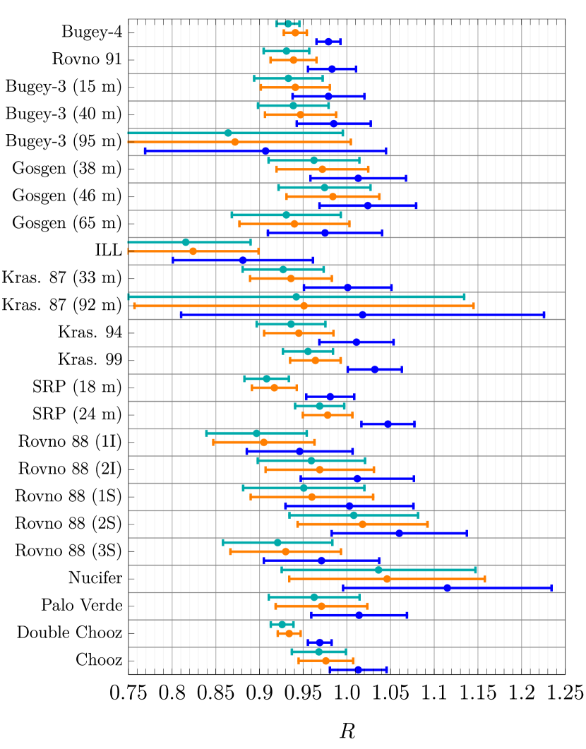
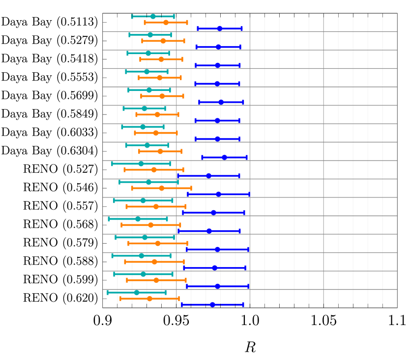
We depict the data discussed above in Figs. 18 and 18. The orange data points represent the ratio of measured IBD rates relative to the prediction calculated using the HM flux model. The blue data points are the same using the ab initio fluxes; the dark cyan points employ the HKSS fluxes. The depicted error bands are experimental only; theoretical uncertainty is of order .
As discussed in Sec. II, the reduction of the antineutrino flux from 235U, in particular, in the ab initio fluxes results in a diminished predicted IBD rate, implying larger experiment-to-prediction ratios. On the other hand, the HKSS fluxes almost universally result in a higher predicted flux, resulting in a diminished ratio .
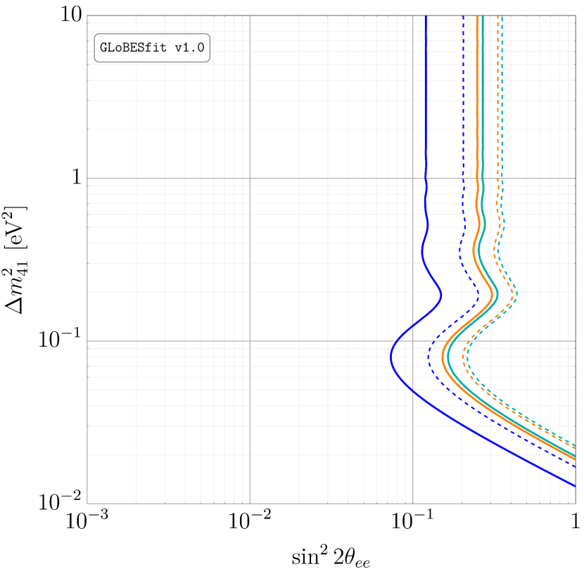
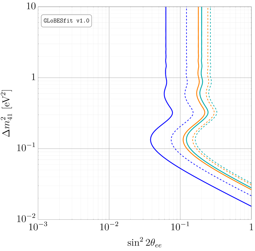
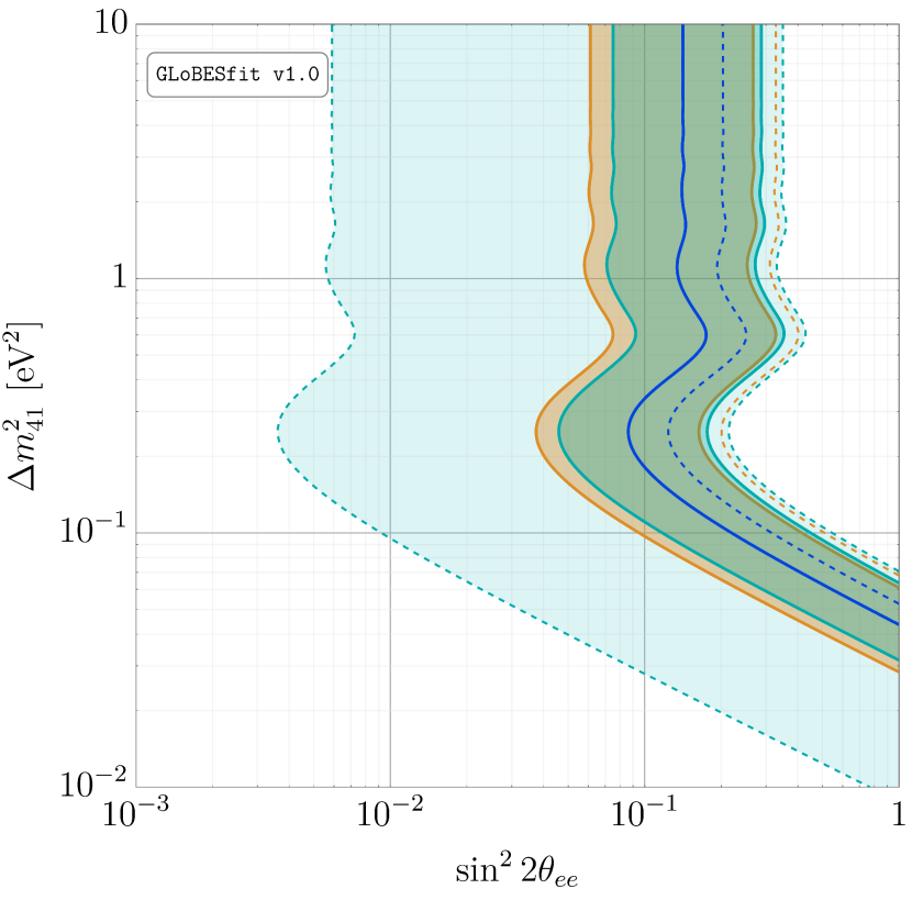
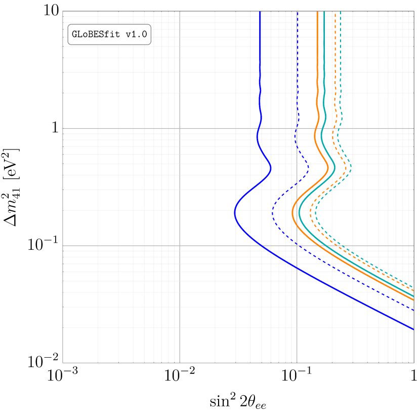
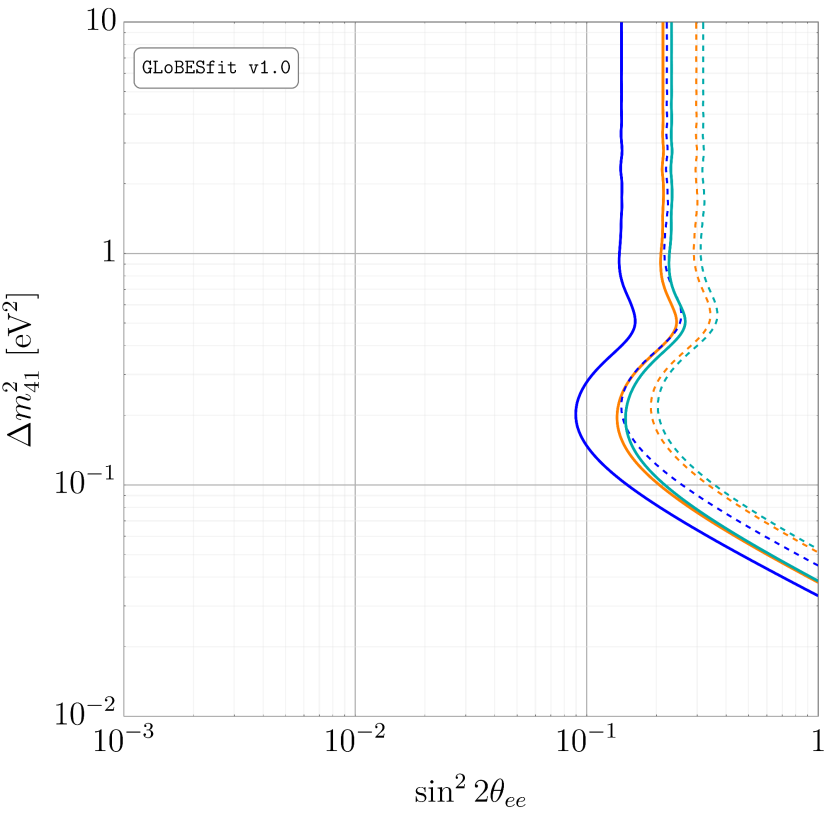
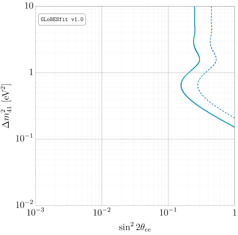
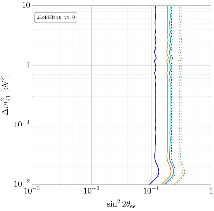
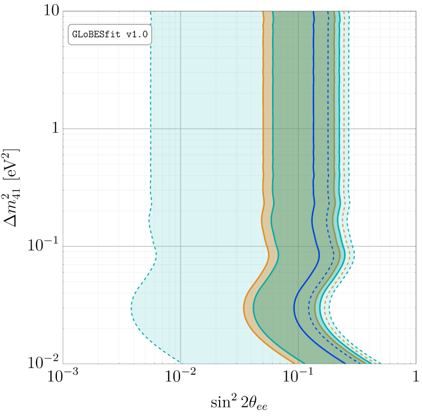
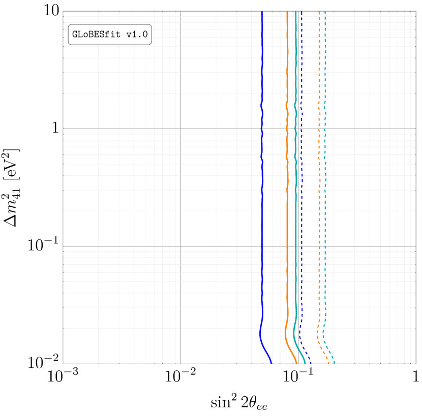
For each group of correlated measurements, we show the 68.3% and 95% confidence level (C.L.) contours derived for each flux model with solid and dashed curves, respectively, in Figs. 2-16; the captions detail which experiments are depicted therein. Results using the HM fluxes are shown in orange; those using the ab initio fluxes are show in blue; and those using the HKSS fluxes are shown in dark cyan.
In Tables 1, 2 and 3, we tabulate relevant statistics for our analyses using the HM, ab initio and HKSS fluxes, respectively. Specifically, we show the minimum value of the for each group of experiments, , as well as the in the limit of no mixing with a sterile neutrino, . The difference between these is used to determine the -value for each group of experiments, assuming these are chi-squared distributed.
| Measurements | |||||
| Bugey-4/Rovno 91 | 4.6 | 2 | 0.10 | 1.6 | |
| Bugey-3 | 1.8 | 0.29 | 3 | 0.48 | 0.71 |
| Gösgen/ILL | 3.9 | 2.4 | 4 | 0.49 | 0.69 |
| Krasnoyarsk 87 | 1.4 | 2 | 0.50 | 0.68 | |
| Krasnoyarsk 94 | 1.4 | 0.0 | 1 | 0.50 | 0.67 |
| Krasnoyarsk 99 | 0.97 | 0.0 | 1 | 0.62 | 0.5 |
| Savannah River, 18 m | 5.6 | 0.0 | 1 | 1.9 | |
| Savannah River, 24 m | 0.38 | 0.0 | 1 | 0.83 | 0.22 |
| Rovno 88 | 3.0 | 1.4 | 5 | 0.46 | 0.74 |
| Nucifer | 0.18 | 0.18 | 1 | ||
| Palo Verde | 0.0 | 1 | |||
| Double Chooz | 5.9 | 0.0 | 1 | 1.9 | |
| Chooz | 0.45 | 0.45 | 1 | ||
| Daya Bay | 12.5 | 8.2 | 8 | 0.12 | 1.6 |
| RENO | 9.7 | 5.2 | 8 | 0.11 | 1.6 |
| All SBL | 14.9 | 7.9 | 21 | 2.2 | |
| All MBL | 29.6 | 18.6 | 19 | 2.9 | |
| All | 39.7 | 31.2 | 40 | 2.5 |
| Measurement(s) | |||||
| Bugey-4/Rovno 91 | 0.59 | 2 | 0.74 | 0.33 | |
| Bugey-3 | 0.50 | 0.27 | 3 | 0.89 | 0.14 |
| Gösgen/ILL | 2.7 | 2.7 | 4 | 0.96 | 0.05 |
| Krasnoyarsk 87 | 2 | ||||
| Krasnoyarsk 94 | 0.06 | 0.05 | 1 | ||
| Krasnoyarsk 99 | 0.77 | 0.76 | 1 | ||
| Savannah River, 18 m | 0.29 | 0.0 | 1 | 0.86 | 0.17 |
| Savannah River, 24 m | 1.7 | 1.7 | 1 | ||
| Rovno 88 | 1.9 | 1.8 | 5 | 0.95 | 0.07 |
| Nucifer | 0.18 | 0.18 | 1 | ||
| Palo Verde | 0.46 | 0.46 | 1 | ||
| Double Chooz | 1.2 | 1 | 0.55 | 0.60 | |
| Chooz | 2.6 | 2.6 | 1 | ||
| Daya Bay | 4.2 | 4.2 | 8 | ||
| RENO | 5.9 | 5.5 | 8 | 0.80 | 0.25 |
| All SBL | 11.2 | 9.9 | 21 | 0.52 | 0.65 |
| All MBL | 19.5 | 17.2 | 19 | 0.30 | 1.20 |
| All | 30.5 | 29.3 | 40 | 0.57 | 0.56 |
| Measurements | |||||
| Bugey-4/Rovno 91 | 5.2 | 0.0 | 2 | 1.8 | |
| Bugey-3 | 2.1 | 0.26 | 3 | 0.40 | 0.84 |
| Gösgen/ILL | 4.1 | 2.2 | 4 | 0.38 | 0.87 |
| Krasnoyarsk 87 | 1.7 | 2 | 0.42 | 0.81 | |
| Krasnoyarsk 94 | 1.8 | 0.0 | 1 | 0.41 | 0.82 |
| Krasnoyarsk 99 | 1.4 | 0.0 | 1 | 0.50 | 0.67 |
| Savannah River, 18 m | 6.4 | 0.0 | 1 | 2.0 | |
| Savannah River, 24 m | 0.70 | 0.0 | 1 | 0.70 | 0.38 |
| Rovno 88 | 3.3 | 1.3 | 5 | 0.37 | 0.90 |
| Nucifer | 0.18 | 0.18 | 1 | ||
| Palo Verde | 0.04 | 0.0 | 1 | 0.98 | 0.03 |
| Double Chooz | 6.4 | 0.0 | 1 | 2.1 | |
| Chooz | 0.20 | 0.20 | 1 | ||
| Daya Bay | 13.4 | 8.2 | 8 | 1.8 | |
| RENO | 10.3 | 5.2 | 8 | 1.8 | |
| All SBL | 15.5 | 8.0 | 21 | 2.3 | |
| All MBL | 30.2 | 18.6 | 19 | 3.0 | |
| All | 40.3 | 31.1 | 40 | 2.6 |
IV.2 Combining Experiments
To analyze all of these experiments simultaneously, we combine the uncertainties on the integrated rate experiments into one covariance matrix, the elements of which are given by correlated and uncorrelated uncertainties described in Sec. III. We use separate covariance matrices for Daya Bay and RENO, which have been provided by the respective collaborations. We incorporate systematic uncertainties stemming from the flux predictions via four nuisance parameters (one for each of 235U, 238U, 239Pu and 241Pu), which we bundle into a vector . These flux predictions are correlated; we account for these correlations using the covariance matrices discussed in Sec. II.
The chi-squared function we employ has the following form:
| (IV.1) |
where is the vector of experimental ratios and is the vector of predicted ratios. Our treatment of theoretical uncertainties has been previously described in Sec. II; the theoretical covariance matrix accounts for these in our calculations. Furthermore, is the covariance matrix describing experimental uncertainties. We minimize over for each point in – parameter space.
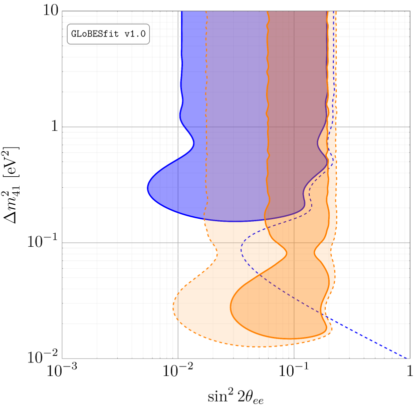
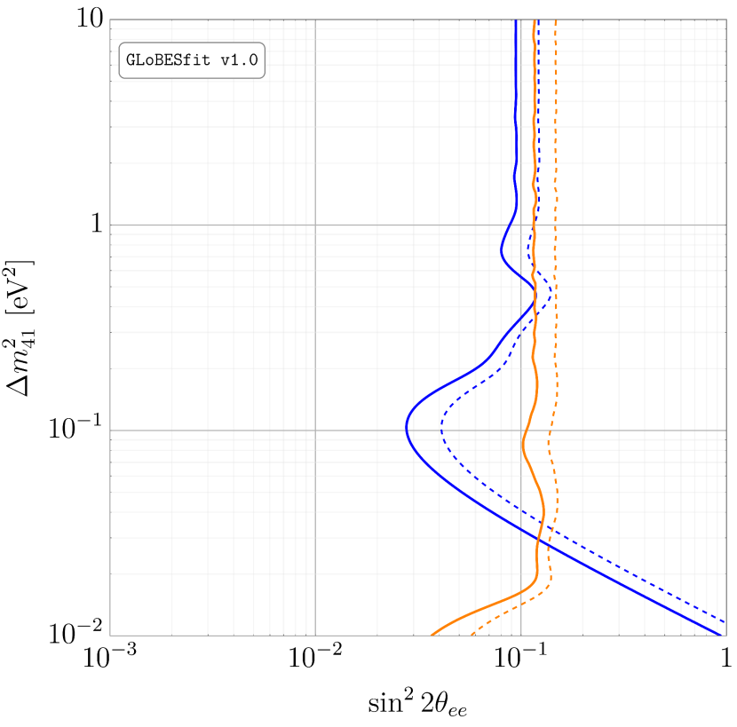
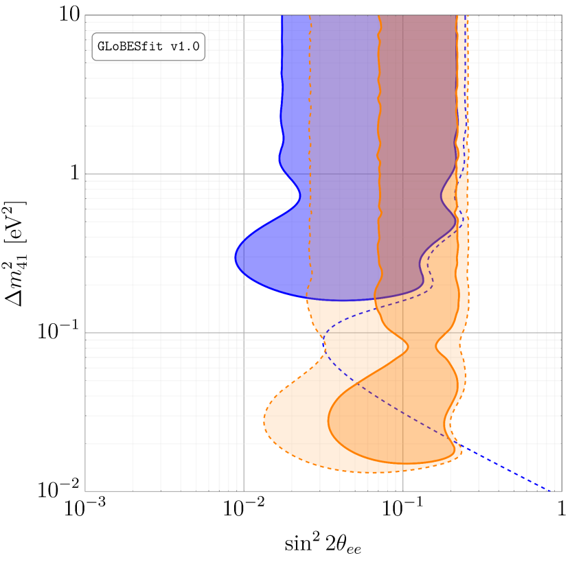
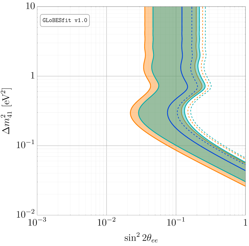
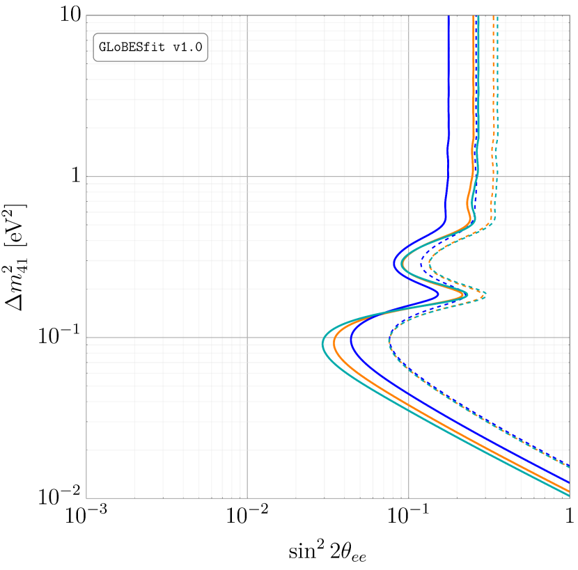
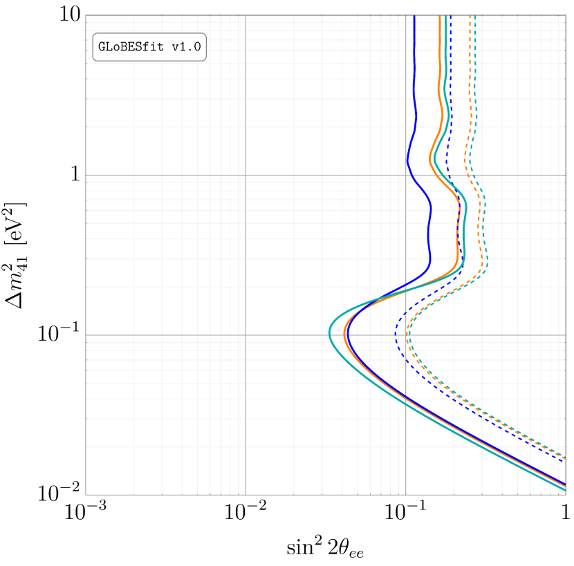
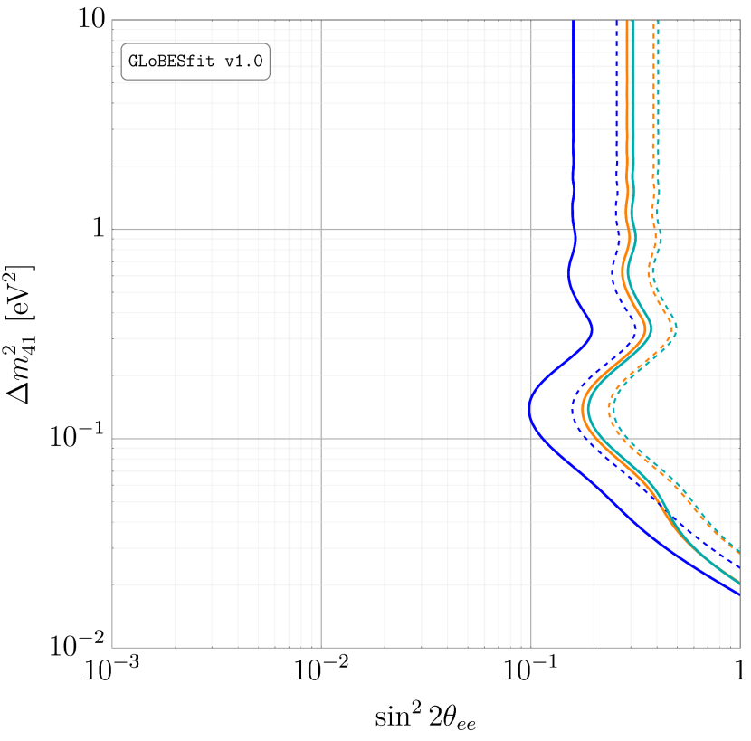
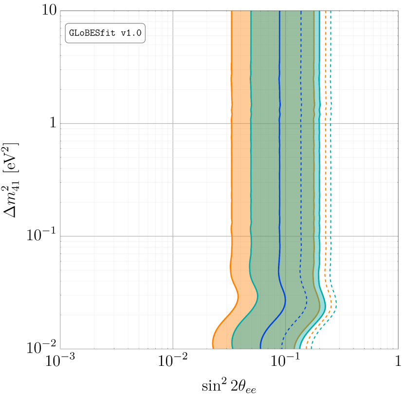
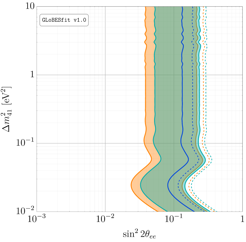
In Figs. 19, 20 and 21, we separately show the regions preferred by short-baseline (SBL) and medium-baseline (MBL) experiments using the HM, ab initio and HKSS fluxes, respectively. In each figure, we show SBL experiments in blue and MBL experiments in orange. Solid contours represent 95% C.L., whereas dashed contours represent 99% C.L. Relevant statistics are compiled in Tables 1-3.
In each case, the MBL experiments prefer a smaller value of than the SBL experiments, as one would expect. In the region above eV2, we see that the MBL experiments are generally consistent with the region preferred by the SBL experiments. Both SBL and MBL experiments separately indicate evidence for a sterile neutrino for the HM and HKSS flux models, though the latter is stronger than the former. Conversely, the ab initio fluxes are much more indifferent to the existence of a sterile neutrino; the 95% C.L. curves do not close for either SBL or MBL experiments, as can be seen from Fig. 20.
In Fig. 22, we show results from combining all SBL and MBL reactor experiments for all flux models we have considered. The solid and dashed curves depict the 95% and 99% C.L. regions, respectively. As before, the HM fluxes are shown in orange; the ab initio fluxes are show in blue; and the HKSS fluxes are shown in dark cyan.
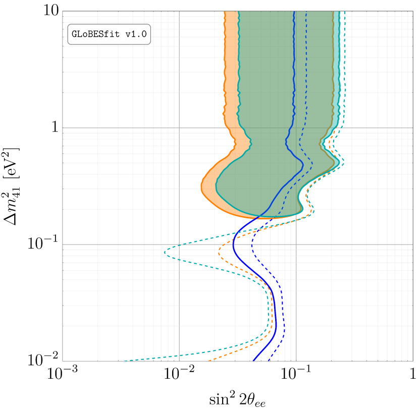
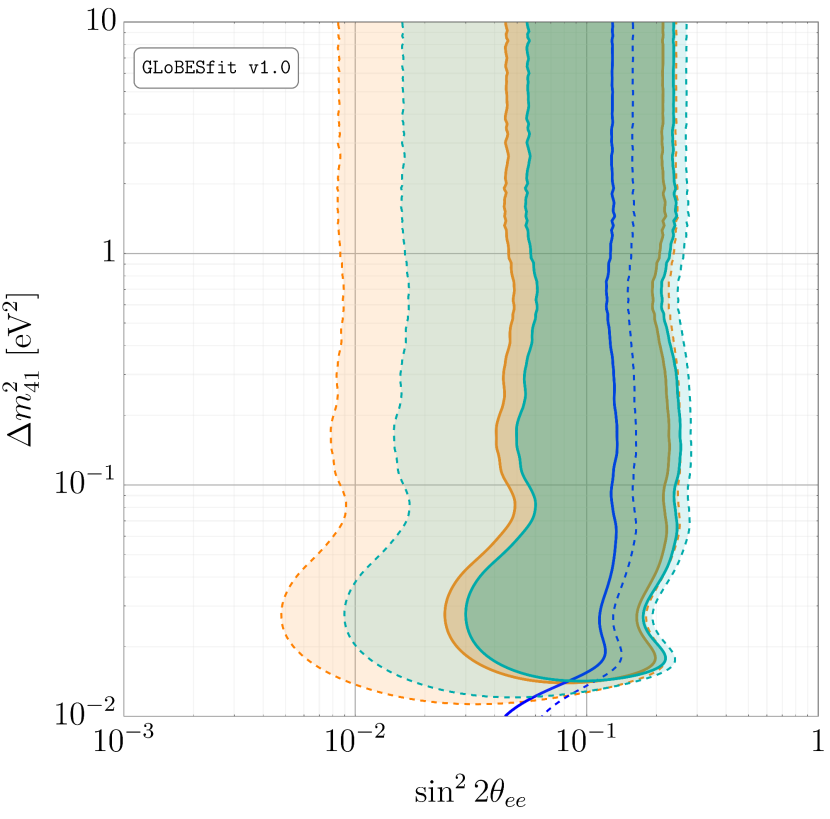
Using the ab initio fluxes decreases the global preference for a sterile neutrino relative to the HM fluxes: the evidence decreases from to . The reason for this, as we have mentioned, is that the overall flux normalization for the ab initio flux prediction for 235U is less than the corresponding HM prediction. Therefore, the ab initio expected IBD rates are less than the HM rates, so the evidence for a sterile neutrino is diminished. Moreover, recall that assigning the HM uncertainties to the ab initio flux predictions is optimistic; the true uncertainties associated with the calculation are assuredly larger than the that we have ascribed. Consequently, this flux model is consistent with no sterile neutrino oscillation.
On the other hand, using the HKSS fluxes increases the global preference for a sterile neutrino: the evidence increases slightly from to . The effect of including first-forbidden decays is to increase the expected flux in the region around MeV; the conversion process thus produces a higher overall antineutrino flux, implying a larger deficit than for the HM fluxes. Additionally, the inclusion of first-forbidden decays has not dramatically increased the uncertainty budget of this calculation, as had been speculated may happen Hayes et al. (2014).
The observation of this diverging preference for a sterile neutrino is one of the central conclusions of this work. Clearly, at most one of these flux predictions is correct; determining which is paramount if the community wishes to determine how to best pursue this anomaly in the coming decade. It is critical to note that these predictions are ultimately derived from experimental measurements — the conversion method requires reliable uranium and plutonium fission spectra, and the ab initio method requires precisely known cumulative fission yields and decay strengths. Perhaps the most critical step to be taken in improving the antineutrino flux predictions is to improve the underlying data on which they are based.
It is important to stress that HKSS represents the first attempt to systematically include forbidden decays in flux predictions and there are a number of caveats one might raise with respect to the methods used. The shell model works best for spherical nuclei with near-magic numbers of nucleons, properties decidedly absent in many fission fragments. Moreover, the shape factors reported in Ref. Hayen et al. (2019) are larger than any observed shape factors. It is worthwhile to point out that for nuclei with non-unique forbidden decays for which the beta spectrum has been measured, the overall spectral shapes are close to the allowed one. A similar caveat applies to Ref. Hayes et al. (2014): if the operator which causes by far the largest effect on the neutrino flux, , were to dominate a given beta decay branch, then a bimodal beta spectrum would result. However, this never has been observed. This may all be indicating that the concerns about forbidden decays in computing reactor neutrino fluxes may have been overstated.
Temporal Cut: Experiments from the 2010s
Given the scarcity of experimental information that accompanies reports of older reactor experiments, one can reasonably ask how the evidence for the existence of a sterile neutrino changes if only recent experiments are included in our analysis. We introduce an ad hoc temporal cut on these reactor data – for concreteness, we only consider experiments from the 2010s, i.e., Nucifer, Double Chooz, Daya Bay and RENO – and derive the constraints shown in Fig. 23. As in previous figures, the 95% (99%) C.L. contour is shown in solid (dashed), and we simultaneously show results using the HM (orange), ab initio (blue) and HKSS (dark cyan) flux predictions. Relevant statistics are shown in Table 5.
Making this cut removes most SBL experiments, so the barycenters of the fits shift to smaller values of . Imposing this cut increases the evidence for a sterile neutrino for all three flux models. For the HM and HKSS flux models, the evidence increases to and , constituting modestly strong evidence. On the other hand, the significance for the ab initio flux model rises to .
To counteract the disproportionately high relevance of MBL experiments in this fit, we impose an additional ad hoc prior requiring eV2 and repeat the analysis. The resulting statistics are shown in Table 5. The evidence is weakened by imposing this prior, but the same basic trend emerges: the HM and HKSS flux models prefer a sterile neutrino at , while the ab initio fluxes show negligible preference.
| Flux Model | d.o.f. | ||||
|---|---|---|---|---|---|
| HM | 24.8 | 14.7 | 14 | 2.7 | |
| Ab Initio | 13.3 | 11.5 | 14 | 0.42 | 0.81 |
| HKSS | 25.6 | 14.8 | 14 | 2.8 |
| Flux Model | d.o.f. | ||||
|---|---|---|---|---|---|
| HM | 24.8 | 16.3 | 14 | 2.4 | |
| Ab Initio | 13.3 | 12.8 | 14 | 0.78 | 0.28 |
| HKSS | 25.6 | 16.2 | 14 | 2.6 |
IV.3 Alternate Analysis: Rescaling the HM Fluxes
We consider an alternative to the sterile-neutrino hypothesis: that the data can be explained by simply rescaling the HM fluxes. In particular, we only consider the two dominant fissile isotopes – 235U and 239Pu – and introduce a rescaling factor of each, respectively and . Similar analyses have been performed in Refs. An et al. (2017c); Giunti et al. (2017); Gebre et al. (2018); Bak et al. (2019); Gariazzo et al. (2018); Giunti et al. (2019a); Adey et al. (2019a). We scan over the – plane in order to determine the extent to which the data prefer a rescaling of the HM fluxes and to determine if this is a more compelling explanation of reactor rate deficits than introducing a sterile neutrino. As in our sterile neutrino analyses, we treat systematics from 238U and 241Pu using nuisance parameters.
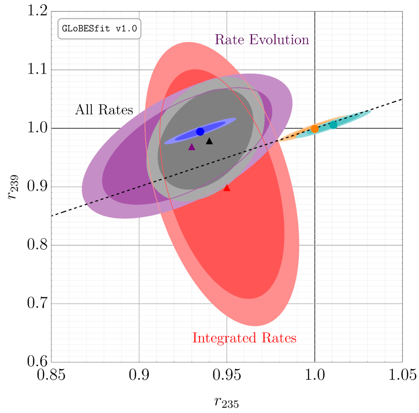
In Fig. 25, we show contours of constant in the – plane for different subsets of reactor experiments. The red regions refer to our analysis of SBL and MBL experiments that measure the total, time-integrated rate (namely, all of the above experiments except for Daya Bay and RENO); the purple regions refer to MBL experiments that measure the IBD rate as the effective fuel fractions change, i.e., Daya Bay and RENO; and the gray regions refer to a combined analysis of all experiments. Dark (light) shading represents the 95% (99%) C.L. region.
In Table 8, we present the minimum value of the (), its value at the point () – indicated by the orange circle in Fig. 25 – and both the corresponding -value and at which the unscaled HM fluxes can be excluded for each dataset. We also show the () preferred region for the HM fluxes in dark (light) orange shading. While the fuel evolution dataset exhibits a moderate but clear preference (), the integrated rate dataset presents evidence in favor of rescaling the HM flux predictions. Taken together, these data present evidence for this hypothesis, with the 235U flux, again, being particularly suspect.
| Analysis | d.o.f. | ||||
|---|---|---|---|---|---|
| Fuel Evolution | 25.8 | 9.0 | 14 | 3.7 | |
| Integrated Rate | 40.7 | 17.8 | 22 | 4.4 | |
| All | 62.6 | 28.0 | 38 | 5.5 |
| Analysis | ||||||
|---|---|---|---|---|---|---|
| Fuel Evolution | 9.4 | 0.83 | 0.22 | 30.8 | 4.3 | |
| Integrated Rate | 19.2 | 0.49 | 0.69 | 49.6 | 5.3 | |
| All | 28.3 | 0.86 | 0.18 | 75.0 | 6.5 |
| Analysis | |||
|---|---|---|---|
| Fuel Evolution | 1.6 | 0.45 | 0.76 |
| Integrated Rate | 0.20 | 0.90 | 0.12 |
| All | 1.8 | 0.42 | 0.81 |
On the other hand, we can directly compare how the ab initio and HKSS flux models compare to this rescaling of the HM fluxes. The blue and dark cyan circles, respectively, represent the relative sizes of the 235U and 239Pu isotopic IBD fluxes as compared to the HM prediction, calculated using our results from Sec. II. As for the HM fluxes, the appropriately colored regions represent the (dark) and (light) regions for these flux models. These three models generally agree on the flux from 239Pu fissions, but disagree quite severely for 235U, with the ab initio fluxes presenting a 6% deficit and the HKSS fluxes presenting a 1% enhancement with respect to HM. We quantify this in Table 8, where we show how these alternate flux predictions compare to freely rescaling the 235U and 239Pu fluxes.
Unsurprisingly, we find that the ab initio fluxes are consistent with the best-fit points from these analyses; the tension between them fails to surpass for any analysis we have performed. Conversely, the data strongly disfavor the HKSS fluxes: while the fuel evolution data exhibit tension, the integrated rate experiments present tension, and all experiments together present tension with this flux model. This again underscores the need to revisit the data that underpin these flux predictions.
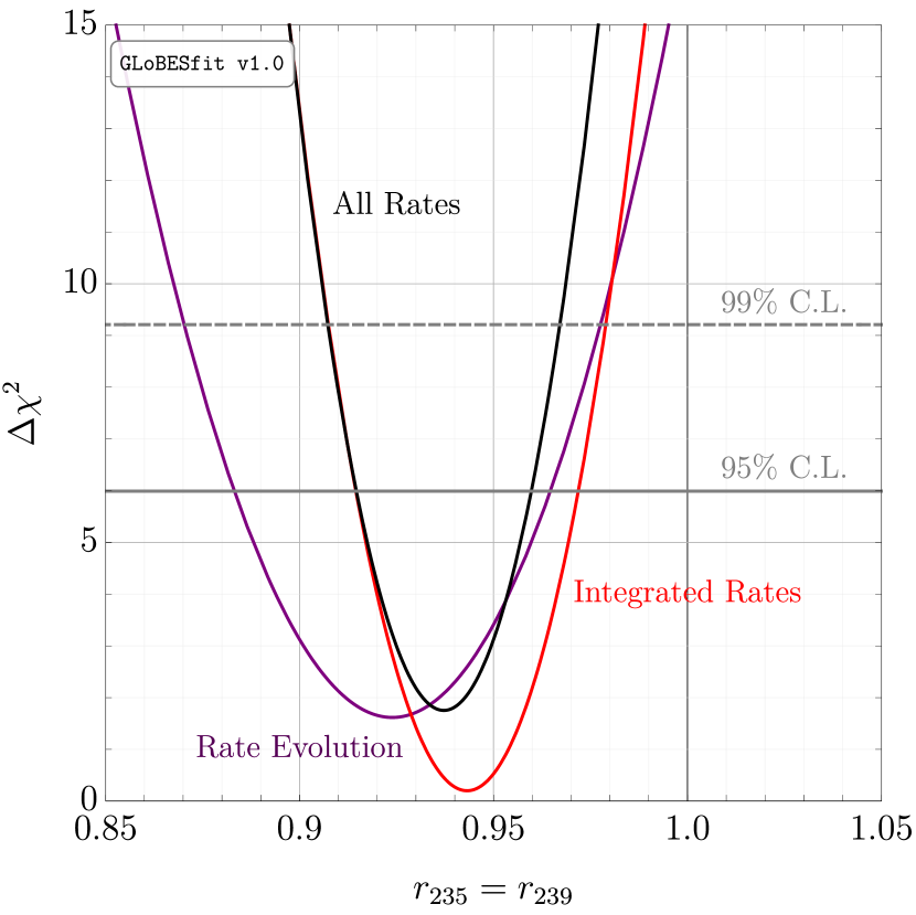
An interesting subset of the rescaling hypothesis is to consider and being rescaled by the same factor. The line along which is shown in black dashing in Fig. 25. In Fig. 25, we show the values of relative to the minimum value in the entire – plane as a function of . Shown are the respective curves for integrated rate (red), fuel evolution (purple) and all experiments (black). The solid (dashed) gray, horizontal line is the 95% (99%) C.L. exclusion limit, calculated for two degrees of freedom; we present this as a subspace of the – plane of Fig. 25, and not necessarily as a separate hypothesis.
In Table 8, we show the minimum value of along this one-dimensional subspace, , the corresponding value and equivalent number of . The data are modestly consistent with a uniform rescaling of the 235U and 239Pu fluxes; a nonuniform rescaling of the 235U and 239Pu fluxes is preferred in an absolute sense, but not dramatically so. None of these analyses excludes a uniform rescaling of the HM fluxes by more than .
We compare the sterile neutrino hypothesis and the rescaled-HM-fluxes hypothesis. For the former, we find /d.of. = 31.1/38, implying (or ). For the latter, we find /d.o.f. = 28.0/38 and (). Clearly, the data mildly prefer for the fluxes to be independently rescaled over introducing a sterile neutrino. This is unsurprising: the the sterile neutrino hypothesis can be mapped onto rescaled-HM-fluxes hypothesis, assuming is sufficiently large that its corresponding oscillations average out at all experiments. Because the former is a subset of the latter, it cannot be more strongly preferred. Introducing the ad hoc restriction that eV2 to ensure that oscillations would average out at all experiments, we find /d.o.f. = 32.3/39 and ().777We take the number of degrees of freedom to be 39 here. If is large enough for oscillations to average out, then its value cannot be measured and it is not a relevant degree of freedom.
V Spectrum Experiments
In this section, we discuss the experiments that enter into our spectral analyses. Unlike the rate experiments, these are all taken to be mutually uncorrelated. Given the increase in the complexity of each measurement – i.e., given that we are considering event spectra instead of integrated event rates – the systematics become much richer than in the previous section(s). Consequently, we discuss the statistical analysis of each experiment separately in what follows.
For these analyses, we exclusively employ the ab initio flux predictions. The reason for this is that, because we are interested in the ratios of spectra, one should expect that the choice of flux model does not affect the results of such a study. One could just as easily use the HM or HKSS fluxes; the result are essentially indistinguishable.
We have limited our analyses to considering Bugey-3 Declais et al. (1995), DANSS Alekseev et al. (2018), Daya Bay Adey et al. (2018), Double Chooz De Kerret et al. (2019), NEOS Ko et al. (2017) and RENO Bak et al. (2019). While the short-baseline reactor experiments PROSPECT and STEREO have produced early results, these are not yet competitive with other experiments in the best-fit region around eV2, so we do not include them at this time. Additional data releases are expected in the near future for both experiments,888While this manuscript was being prepared, Ref. Almazán Molina et al. (2019) appeared on the preprint arXiv. We will include these data in future analyses, but we have not included them here. as well as the SoLid experiment Ryder (2015); we look forward to including all of these in future versions of GLoBESfit.
V.1 Bugey-3
Implementation in GLoBES
Based on design specifications for a 900 MWe series reactor vessel described in Ref. Jacquemain et al. (2015), we assume that the height of the active volume of the reactor core at Bugey-3 is 3.66 m tall with a radius of 1.5 m. We further assume that antineutrino production is uniform vertically999In reality this follows a distribution with being in the center of the reactor, but since the reactor center and detector position are essentially at the same level, this has no practical impact on the baseline distribution. and azimuthally, but that the radial distribution is given by a zeroth-order cylindrical Bessel function whose first zero lies at the edge of the core.
We only consider the antineutrino spectra measured at the 15 m and 40 m positions. The spectral measurement at 95 m is sufficiently imprecise that we do not expect to gain appreciable sensitivity to a sterile neutrino through its inclusion; this is borne out in Fig. 16 of Ref. Declais et al. (1995). Ref. Declais et al. (1995) states that the detector modules used in the experiment are comprised of 98 separate cm3 segments arranged in a grid; the total dimensions of the modules are cm3. The detector in the 15 m position is comprised of one such detector module, whereas the detector in the 40 m position is comprised of two of these, having total dimension cm3. We find that our results are insensitive to the exact relative orientation of either detector and the core.
We precompute the oscillation probabilities at both positions using the geometries outlined above. The quantity of interest is the flux-averaged value of at each experiment, where
| (V.1) |
is independent of the experimental geometry. Note that this definition of assumes that lengths are given in km, which is the expectation in GLoBES. We define this average to be , and discuss it in more detail in the Appendix (see Eq. (A.8) and the surrounding discussion). We precompute in intervals of 0.01 in over the range .
The two positions are included with two separate AEDL experiments in GLoBESfit. We fix @time, @power, @norm and $target_mass to be 1.0 for both positions, and the spectrum is sampled in 25 bins on [2.8, 7.8] MeV in antineutrino energy, corresponding to [1.0, 6.0] MeV in positron energy. As for our rate analyses, we the energy resolution to be . We set the values of $lengthtab for each to the appropriate value of for each position; we calculate these to be 14.93 m and 39.96 m. We take the effective fission fractions to be
for the duration of the experiment for both the 15 m and 40 m positions.
Statistical Analysis
The upper panel of Fig. 15 of Ref. Declais et al. (1995) shows the ratio of the spectrum measured at 40 m relative to that measured at 15 m. We have digitized this figure and the depicted statistical uncertainties for use in our analyses; we reproduce these data in Fig. 38(a) in Appendix C. In addition to these statistical uncertainties, the collaboration also claims a 2.0% systematic uncertainty on the relative normalization of the two spectra. We have also accounted for a 2.0% energy scale uncertainty for each position and have assumed that these are totally uncorrelated. These are included in our analyses via the GLoBES function glbShiftEnergyScale; see the GLoBES manual for a description of this function Huber et al. (2005, 2007).
We utilize a chi-squared function of the following form:
| (V.2) |
where is the experimental spectrum and is the ratio predicted using GLoBES, assuming the existence of a sterile neutrino with mixing angle and mass-squared splitting . The covariance matrix includes statistical uncertainties and the 2.0% normalization uncertainty. The nuisance parameters and correspond to variations in the energy scale at 15 m and 40 m, respectively, with uncertainties of 2.0% apiece. In our fits, we minimize over these nuisance parameters for each value of and .
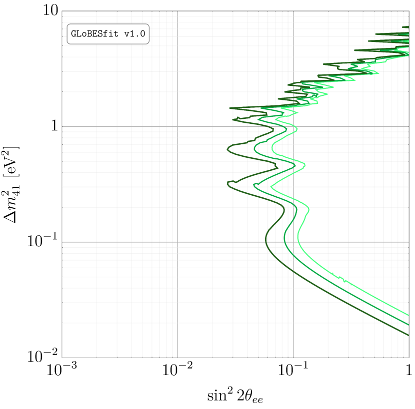
The results of our benchmark sterile neutrino analysis are shown in Fig. 26. The dark green, green and dark green contours represent the 95%, 99% and 99.9% C.L. contours, respectively. Relevant statistics are summarized in Table 9. Bugey-3 shows a modest preference for a sterile neutrino; we find that the evidence rises to the level of .
V.2 DANSS
Implementation in GLoBES
The DANSS Alekseev et al. (2018) reactor core is a 3.7-meter-tall cylinder with a diameter of 3.2 m. We assume production to be uniformly distributed, but that the radial distribution is given by the zeroth-order cylindrical Bessel function with zero at edge of core; we sample the vertical extent of the core following the burning profile in Ref. Danilov . The detector is a 1 m3 cube located directly underneath the axis of the core; in our analyses, the centers of the core and the detector are taken to be either 10.7 m or 12.7 m apart, and we are ultimately interested in the ratio of the spectra obtained at these distances. We calculate the oscillation probabilities as described in Appendix A. We calculate (see Eq. (A.8)) on the range in intervals of 0.01 in for both the top ( m) and bottom ( m) positions.
We introduce separate experiments in GLoBESfit for the upper and lower positions at DANSS.101010The collaboration also publishes the ratio of events in a middle position relative to the upper position Alekseev et al. (2018). Given that these are nontrivially correlated with the lower-to-upper ratio and that these are not likely to dramatically affect the final exclusion, we ignore these data. Since we are interested in the ratio of the spectra in the upper and lower positions and not in the absolute number of events, we fix @time, @power, @norm and $target_mass to be 1.0 for both positions. The main difference, of course, is the values of $lengthtab; this is given by the appropriate value of . These are determined to be 10.68 m and 12.69 m for the upper and lower positions, respectively, based on the previously described geometry.
The spectrum is calculated for 24 bins on [2.8, 8.8] MeV in antineutrino energy, corresponding to [1.0, 7.0] MeV in positron energy. We estimate the energy resolution from Table 1 of Ref. Alekseev et al. (2018); we fit the width to a function of the form and find . We use the following fuel fractions:
| (V.3) |
These are the fuel fractions during the middle of a VVER-1000 reactor operating cycle as presented in Table 1 of Ref. Kopeikin (2012).
Statistical Analysis
Table 2 in Ref. Alekseev et al. (2018) tabulates the bottom/top spectral ratio, as well as the statistical errors on these ratios; we reproduce these data in Fig. 38(b) in Appendix C. The DANSS collaboration has not published a thorough analysis of their systematic uncertainties, but the impact of these have been estimated in the final result. Specifically, the following systematics have been included:
-
•
The energy scale uncertainty is taken to be 2.0%, and is fully correlated between the upper and lower configurations. This systematic is included via the GLoBES function glbShiftEnergyScale. A nuisance parameter is introduced corresponding to this energy scale shift.
-
•
The uncertainty on the ratio of for the upper and lower positions is taken to be 2.0%. This introduces correlations between the spectral ratios.
The following chi-squared function is employed in these analyses:
| (V.4) |
where is the measured bottom/top ratio, is the prediction of the same from GLoBES and is the covariance matrix describing these data. The nuisance parameter associated with the energy scale is and the corresponding uncertainty is . In our analysis, we minimize over for each point in the – plane.
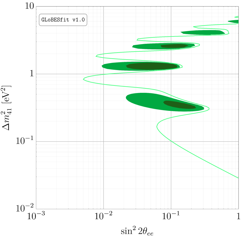
The results of our analysis are shown in Fig. 27. The dark green, green and dark green contours represent the 95%, 99% and 99.9% C.L. contours, respectively. Relevant statistics are summarized in Table 9. DANSS presents the most compelling single piece of evidence for a sterile neutrino of the experiments that we have considered – the evidence rises to the level of .
V.3 Daya Bay
Implementation in GLoBES
Daya Bay consists of an array of eight antineutrino detectors (ADs) and six nuclear reactors. Our analysis of the antineutrino spectrum at Daya Day is based on the 1958-day data release in Ref. Adey et al. (2018). The data have been taken in three phases, corresponding to the active number of ADs: sequentially six (6AD; 217 days), eight (8AD; 1524 days) and seven (7AD; 217 days).
In their 1230-day data release An et al. (2017b), the collaboration reports the average power of each reactor core during the 6AD period and in the first 1013 days of the 8AD period; similar figures have not been published for the 1958-day data. We assume that (1) the average powers during the entire 8AD period are given by the average powers during the first 1013 days, and (2) that the average powers of during the 7AD period are equal to those from the 6AD period. We do not expect these assumptions to dramatically affect the outcome of this analysis, but we look forward to updating this in the future. The average powers during the 6AD and 8AD periods from the 1230-day data are tabulated in Table 14.
The distances between pairs of reactors and detectors are tabulated in Table I of Ref. An et al. (2017b); we tabulate these in Table 13. We treat the reactor cores as being point-like, but the ADs are treated as 3-meter wide targets, the stated size of the acrylic vessel that contains the Gd-doped liquid scintillator An et al. (2017b). The function (see Eq. (A.8)) for each detector is written as follows:
| (V.5) |
where indexes the reactor cores, indexes the three data-taking periods, is the live-time of detector during period , is the power of core during period and is the distance between detector and core . The detector live-times are given as follows:
-
•
ADs 1-6 have = 217 days; ADs 7 and 8 have = 0 days.
-
•
ADs 1-8 all have = 1013 days.
-
•
ADs 2-8 have = 217 days; AD 1 has = 0 days.
The oscillation probabilities are precomputed using a look-up table for each detector, for values of with a grid spacing of 0.001.
There are five factors that differentiate each detector:
-
1.
For each detector, we define @time = 1.0 but, since not all detectors have been operational for the same amount of time, we fold these differences into the definition of @power. Namely, this is defined to be
(V.6) -
2.
The target masses have subpercent-level differences; these are tabulated in the first row of Table 15 and are accounted for using $target_mass.
-
3.
The total efficiencies of the ADs also vary; these are given in the second row of Table 15. We set @norm to be the stated value of for each detector.
-
4.
The effective baseline of each detector, , is defined via
(V.7) These are tabulated in the third row of Table 15.
-
5.
Lastly, the effective fuel composition visible to each detector varies; these are tabulated in the last four rows of Table 15.
The energy resolution of each detector is taken to be identical. In the supplementary material to Ref. An et al. (2017b), the Daya Bay collaboration publishes the response matrix that they use in their analysis. In principle, we could use the same response matrix here; to cut down on computation time, we parametrize the response using function of the form . We find
Statistical Analysis
The nominal Daya Bay analysis ranges from prompt energies MeV with irregular binning; the first bin is MeV, the last bin is MeV and everything in between is regularly spaced in 0.2-MeV bins. The spectrum at each AD is calculated over MeV in true antineutrino energy in 226 bins. This results in a 0.05-MeV spacing over the visible spectrum; this fine a spacing allows us to recycle our spectrum calculations for our analysis of NEOS, explained in Sec. V.5. These bins are combined at the analysis level to reproduce the Daya Bay binning.
We are ultimately interested in the ratios of total events in EH2 (i.e., AD3 & AD8) and EH3 (AD4-7) to EH1 (AD1, 2), which we call EH2/EH1 and EH3/EH1. The spectrum observed at each EH is determined by simply summing the number of spectrum for each detector in the hall, accounting for the appropriate effective fuel fractions. Taking the ratios of these spectra, which we call and for EH2/EH1 and EH3/EH1, respectively, is then trivial.
We benefit from the extensive data release from the Daya Bay collaboration in the form of supplementary data to Ref. Adey et al. (2018). In particular, the total numbers of observed IBD candidates (signal+background) for each bin in each experimental hall reside in the files DayaBay_IBDPromptSpectrum_EH<N>_1958days.txt, where <N> = 1, 2, 3; the background spectra have also been published and reside in the files DayaBay_BackgroundSpectrum_EH<N>_1958days.txt. We extract the observed ratios and ; we show these data in Figs. 39(a) and 39(b), respectively. These are the basis of our chi-squared, defined as
| (V.8) |
where and have been combined into one vector and is the covariance matrix, which accounts for both statistical and systematic errors including correlations. We describe our estimation of the covariance matrix in what follows.
The number of signal events in any of EH1, EH2 or EH3 (from data), which we call , is given by the difference between the total number of events and the expected number of background events ; here, (= 1, 2, 3) indexes the experimental hall. The uncertainty on is statistical; the event rates are large enough where they can assumed to Gaussian-distributed. The uncertainty on , however, is considered a systematic uncertainty; we discuss it further below. Therefore, the statistical uncertainty on a given element of , which we call , is . The statistical component of the covariance matrix is determined by randomly varying the , calculating the ratios and separately for each bin and determining at the covariance of the resulting pseudodata. The correlation between and is also recorded.
The collaboration provides a list of systematic uncertainties in Table VIII of Ref. An et al. (2017b); in Ref. Adey et al. (2018), it was reported that the uncertainty on the 9Li background has been reduced from 43% to 27% in EH1 and EH2. We have considered the contribution of each of these components, accounting for the stated level of correlations between detectors, reactors and other systematics, using Monte Carlo methods: the fractional change in the event rate is calculated by varying each systematic and the covariance matrix of the resulting pseudodata is recorded. In practice, we find that the largest contributions to the covariance matrix come from (1) variation in the backgrounds, and (2) varying the detector response. Unsurprisingly, the uncertainty on the HM flux predictions is found to be negligible – this is precisely the reason why the ratios of event rates have been used in this analysis.
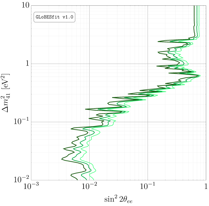
As previously mentioned, the absence of specific information regarding the true average reactor powers and live-times for each detector during each operation period means that our predicted ratios of spectra will not agree with the true ratios, even in the absence of a sterile neutrino. To compensate for this, we introduce two calibration factors, one for each spectral ratio, which are ad hoc attempts to reproduce Daya Bay data; these are introduced via the replacements and . These factors are determined by minimizing the above chi-squared function assuming only three-neutrino oscillations with the best-fit three-neutrino parameters in Ref. Esteban et al. (2019), and are found to be and . A more accurate estimate of the sensitivity can be obtained using more accurate information regarding the cores and detectors.
V.4 Double Chooz
Implementation in GLoBES
Double Chooz consists of two monolithic, Gd-doped liquid scintillator detectors located in the vicinity of two commercial power reactors. The separations between the reactors and the detectors are taken from Fig. 1 of Ref. De Kerret et al. (2019); the distances are tabulated in Table 23. Given the m baselines, we safely assume that both reactors are point-like. However, the detector is taken to have a width of 3 m; this helps to ensure that fast oscillations average out in our calculations, and is consistent with the physical width of the detector.
The collaboration has not published the (relative) average powers of the two reactors during the data collection periods for either the near or far detector; we assume that the average powers are the same, and comment on this further below. We again calculate the quantity as in Eq. (A.13), accounting for both reactors at each detector. This quantity is precomputed in steps of 0.01 in ; we calculate this for for the near detector and for the far detector.
Each detector is separately defined within GLoBES, using the information contained in Table 23. We set @time to the operating time of the detector (in days), @power to 8.5 GW (assumed to be the same for the neat and far detectors) and @norm to be the efficiency. We set lengthtab to the corresponding value of , given by 0.4003 km and 1.052 km for the near and far detectors, respectively. The collaboration reports De Kerret et al. (2019) that the near detector has times as many protons in its Gd-doped target as the far detector does, and times as many protons in its gamma catcher. Given the relative volumes of these two regions, we estimate that the near detector has times as many protons as the far detector. Consequently, we set $targetmass to be 1.0 for the far detector and 1.0044 for the near detector.
The energy spectrum in each detector is calculated in 26 bins between [1.8, 8.3] MeV in antineutrino energy, corresponding to [1.0, 7.5] MeV in prompt energy. The effective fuel fractions are the same as for our rate analysis,
and we again take the energy resolution to be .
Statistical Analysis
Figure 4 of Ref. De Kerret et al. (2019) shows the measured ratio of spectra at the Double Chooz near and far detectors; we reproduce these data in Fig. 38(c) in Appendix C. For our analyses, we have digitized these data and the corresponding statistical uncertainties. We also consider the following sources of systematic uncertainty:
-
•
Detection Uncertainties. These are enumerated in the third column of Table 2 in Ref. De Kerret et al. (2019) and amount to a 0.475% uncertainty, assumed to be correlated between all energy bins.
-
•
Flux Uncertainties. A 0.47% reactor-uncorrelated thermal power uncertainty has also been included. This results in a 0.4% uncertainty on the spectral ratio, assumed to be correlated between all energy bins.
-
•
Backgrounds. Background rates at the near and far detector are given in Table 3 of Ref. De Kerret et al. (2019) and the corresponding spectra are shown in Fig. 3 for both the near and far detectors. From these figures, we estimate the contribution of each background process to the background-subtracted event rate and the corresponding uncertainty using a simple Monte Carlo routine. This procedure yields the background-related uncertainty on the spectrum, including nontrivial correlations.
These are all included into a chi-squared function of the following form:
| (V.9) |
where and are, respectively, the measured and predicted spectral ratios at Double Chooz. We note that we have reweighted the measured data by a factor
i.e., by the ratio of the predicted numbers of events in either detector. The covariance matrix contains the statistical and systematic uncertainties described above.
In the absence of published information regarding the relative powers of the two reactors over the operation of each detector, comparing and can be problematic – it’s unclear what the appropriate three-neutrino-oscillation baseline should be. To address this, we reweight our predicted spectrum by a factor , determined as follows. We calculate assuming only three-neutrino oscillations using the value of measured by Double Chooz in Ref. De Kerret et al. (2019), i.e, . We then replace and minimize over ; we find . We then include this factor in all subsequent calculations.
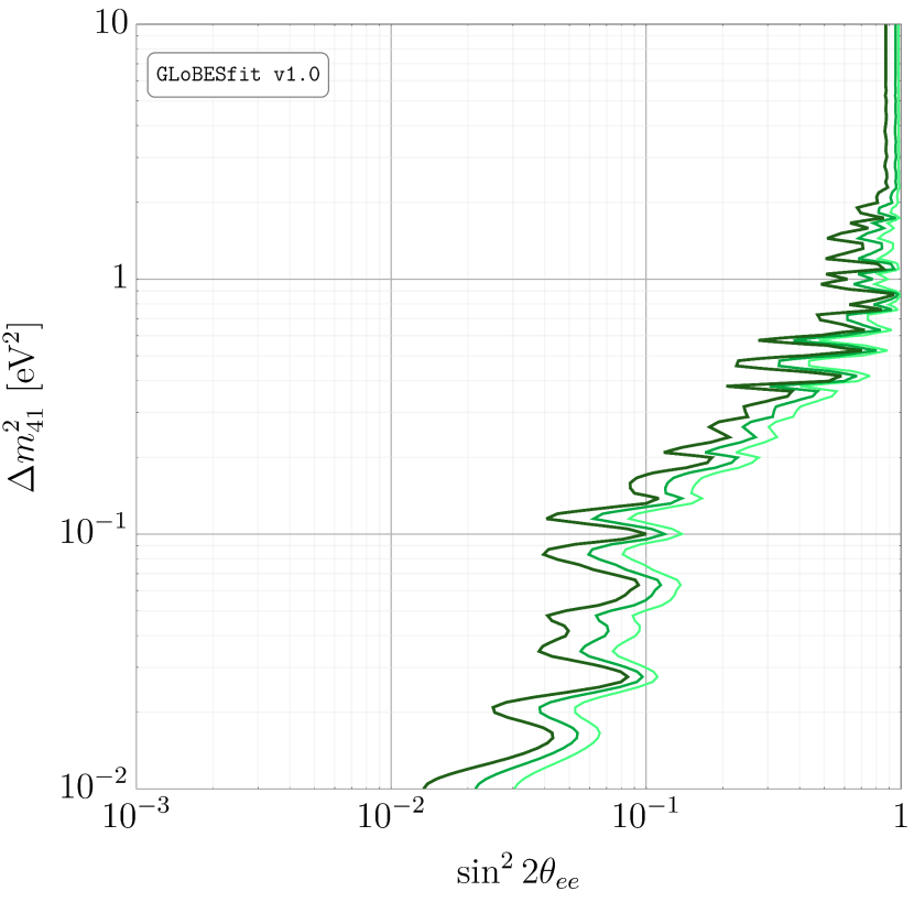
The results of our calculation are shown in Fig. 29.111111We have resumed calculating with , from Ref. Esteban et al. (2019). The dark green, green and dark green contours represent the 95%, 99% and 99.9% C.L. contours, respectively. Relevant statistics are compiled in Table 9. The evidence for a sterile neutrino at Double Chooz is weak – while the data show a clear deficit stemming from nonzero , the data are sufficiently imprecise that any fine structure beyond the expected patter is washed out.
V.5 NEOS
Implementation in GLoBES
Details of the geometry of NEOS are taken from Ref. Ko et al. (2017). The reactor core at unit 5 of the Hanbit Nuclear Power Complex, where NEOS is housed, is 3.1 m in diameter and 3.8 m in height. The detector is located in the plane 10.0 m beneath the center of reactor; labeling the center of core as the origin of our coordinate system and call the axis of the cylinder the axis, the coordinate of the detector is m. The center-to-center distance is 23.7 m; the remaining coordinates of the center of the detector are taken to be m and m. The detector is 1.21-meter-long cylinder with diameter 1.03 m and is oriented so that its axis is in the plane, i.e., the axes of the detector and the core are orthogonal. Ref. Ko et al. (2017) does not further specify the orientation of the detector axis in the plane, but the analysis is not particularly sensitive to this detail, given the size of the detector. For concreteness, we orient the detector along the axis.
We estimate the distribution of baselines (more concretely, the distribution of values between points in the core and the detector) using a simple Monte Carlo routine. The effective length to be m. These distances are also used to calculate the function (Eq. A.8) over the range in steps of 0.01 in .
NEOS, itself, requires one experiment file within GLoBESfit. The NEOS collaboration reports a prompt energy spectrum on MeV. We choose to ignore the last bin, covering MeV, in our analysis; there are very few events in this bin, so we do not expect to lose much information. The NEOS collaboration presents their data in terms of a ratio relative to the antineutrino spectrum measured at the Daya Bay near detectors in Ref. An et al. (2017a); see Fig. 3(c) of Ref. Ko et al. (2017).121212The collaboration also publishes the ratio of their data relative to the HM fluxes; see Fig. 3(b) of Ref. Ko et al. (2017). Given the size of the theoretical uncertainties on the flux predictions and the unexplained spectral features at 1 MeV and 5 MeV, we consider the ratio of measured spectra, even though these have been measured by two different experiments. The spectrum that we use to normalize the NEOS result is the sum of the antineutrino spectra in AD1 and, AD2, i.e., the detectors in EH1. The ratio of NEOS data relative to the Daya Bay spectrum is shown in Fig. 38(d) in Appendix C.
Since we are again interested in a ratio of spectra, @time, @power, @norm and $target_mass are all fixed to be 1.0. We use the same parametrization of the energy resolution at NEOS as Ref. Huber (2017); however, since GLoBES assumes all energies are in GeV, we write the resolution as
| (V.10) |
Lastly, we fix $lengthtab = 0.02369 km, as described above. The spectrum is calculated for each of the four main fissile isotopes, and these are added together, weighted by the relevant fuel fractions Huber (2017); Ko et al. (2017):
Statistical Analysis
The object in which we are ultimately interested is the double ratio of NEOS and Daya Bay spectra, to wit,
| (V.11) |
where is the number of antineutrino events calculated using GLoBES for experiment (= NEOS; DB, EH1) under the assumption of the existence of neutrinos in bin , defined using NEOS’s 0.1-MeV binning. The justification for this is as follows.
As mentioned, the NEOS collaboration normalizes their spectrum relative to the Daya Bay measured flux. The latter has been inferred from the Daya Bay 1230-day data after unfolding three-neutrino oscillations. To properly account for the presence of a fourth neutrino in this denominator, one must first refold the best-fit three-neutrino oscillations before unfolding four-neutrino oscillations, with some assumptions about the new mass and mixing. This amounts to multiplying by the ratio of the expected numbers of events in a given bin at the Daya Bay near detectors with and without a sterile neutrino. Additionally, because the Daya Bay prediction has been rescaled to the NEOS data, there should also appear a factor of the ratio of oscillation probabilities at NEOS with and without oscillations. We are thus led to consider Eq. (V.11), which has been previously considered in Refs. Dentler et al. (2017, 2018).
We use EH1 from Daya Bay to provide the rescaling of the measured flux in Eq. (V.11) in our calculations. The oscillation probabilities at NEOS are calculated assuming that only oscillations into the sterile state are relevant, but the full four-neutrino machinery is applied to Daya Bay. The following chi-squared is used in order to study the extent to which NEOS can probe the existence of a sterile neutrino:
| (V.12) |
where are the NEOS data, is the ratio calculated using GLoBES and is the covariance matrix of these data. As with DANSS, we introduce an explicit nuisance parameter for the energy scale uncertainty, whose uncertainty is nominally 0.5% Ko et al. (2017). This is studied using the GLoBES function glbShiftEnergyScale; in our fits, this parameter is minimized for every point in the sterile neutrino parameter space.
We turn now to the covariance matrix . There are two contributions that we include in this matrix. The first is the statistical uncertainties on the ratio , which are simply read off of Fig. 3(c) in Ref. Ko et al. (2017). The second is the covariance matrix published with the antineutrino spectrum in Ref. An et al. (2017a). Daya Bay publishes their results using a different binning than NEOS; we reformulate the covariance matrix using a simple Monte Carlo routine. Random antineutrino spectra are generated using the Daya Bay spectrum and covariance matrix, including correlations. The antineutrino spectrum that NEOS would see is determined by interpolating these generated spectra to the stated NEOS binning. The contents of these bins using the above-stated energy resolution, and the resulting covariance matrix is calculated.
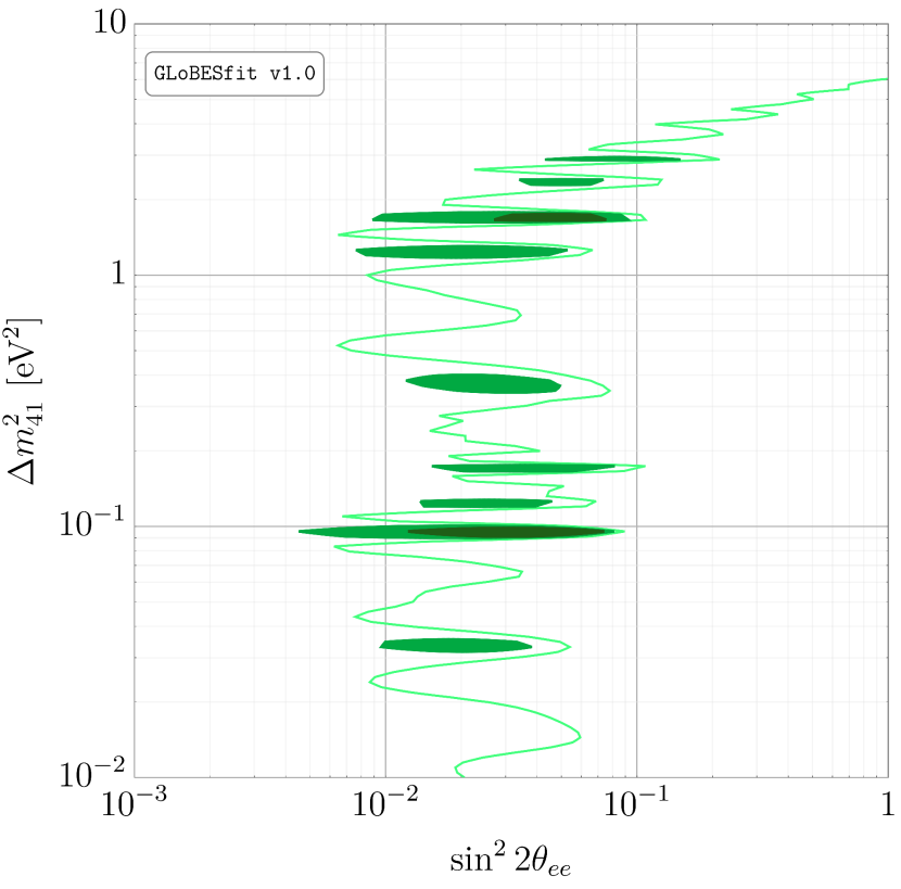
Formally, we need to consider the predicted spectrum given the stated NEOS fuel fraction, not the Daya Bay fuel fraction from which this result is derived. This introduces model dependence on the HM fluxes – and with it, dependence on the uncertainties on these fluxes. These contributions have been included with a similar Monte Carlo routine, but their contribution to the final result is small Huber (2017).
It bears mentioning that the use of the Daya Bay antineutrino spectrum to normalize the NEOS spectrum implies that these experiments are formally correlated with one another. However, we ignore the correlations between these experiments for the following reason. The Daya Bay antineutrino spectrum used at NEOS is based on the 1230-day data; in contrast, the Daya Bay analysis described in Sec. V.3 is based on the 1958-day data. Consequently, it’s difficult to accurately assess the degree of correlation between these data sets. We hope to improve this aspect of our analysis with the collection and dissemination of more data.
The results of this analysis are shown in Fig. 30 The dark green, green and dark green contours represent the 95%, 99% and 99.9% C.L. contours, respectively. Relevant statistics are compiled in Table 9. The sensitivity at low ( eV2) is driven by the use of the Daya Bay spectrum for normalization; NEOS itself drives the sensitivity in the eV2 region. One could, in principle, develop an analysis based on the ratio of NEOS data to the HM flux prediction, the data for which are shown in Fig. 3(b) of Ref. An et al. (2017a); this is precisely what is done in, for instance, Ref. Gariazzo et al. (2018). The exclusions derived there only have support in the region around eV2, but, as mentioned above, are more dependent on the uncertainties of the HM fluxes.
V.6 RENO
Implementation in GLoBES
The geometry of the RENO experiment Bak et al. (2018) has been previously discussed in the context of our rate analysis. We continue to assume that each of the six reactors is point-like, but that both the near and far detector have a width of 3.0 m, to facilitate fast oscillations in averaging out. The distances between either detector and each of the six reactors are shown in Table 18; the average powers of each reactor during the operating period of either detector are shown in Table 19. These data have been obtained from private communications with the collaboration Kim . As with previous experiments, we precalculate (Eq. (A.13)) on a grid with spacing 0.01 in over the range for both detectors.
The near and far detectors are defined as separate experiments within GLoBES. For each, we set @time to the operating time of each detector (in days), @power to the total thermal power from all six reactors and @norm to be the efficiency of each detector. The relevant quantities are tabulated in Table 19. In the absence of any information to the contrary, we assume the detectors to be of equal mass; consequently, we set $target_mass to be 1.0 for each. We set $lengthtab equal to the appropriate value of for the near and far detectors; these values are, respectively, 433.1 m and 1446.9 m.
The antineutrino spectrum is calculated in 29 bins of equal width on [2.1, 7.8] MeV in antineutrino energy, corresponding to [1.3, 7.0] MeV of prompt energy. The RENO data, however, are presented with nonuniform binning; the third- and second-to-last bins have width 0.2 MeV and the last has width 0.3 MeV, whereas all the others have width 0.1 MeV. In our calculations, we manually combine events in our 0.1-MeV wide bins as appropriate to achieve the correct final binning. The effective fission fractions of the four main fissile isotopes for each detector have been provided by the collaboration Kim ; for the near detector, we use
whereas we use
for the far detector. As in the rate analysis, we assume a constant energy resolution of 0.4 MeV.
Statistical Analysis
Our analysis centers around the spectral ratio presented in the bottom panel of Fig. 2 of Ref. Bak et al. (2018). These data and the corresponding statistical uncertainties have been digitized for use in our analyses; we reproduce these data in Fig. 38(e) in Appendix C. Aside from these statistical uncertainties, we consider the following sources of systematic uncertainty:
-
•
Energy Scale. The collaboration claims a 0.15% uncertainty on the experimental energy scale Bak et al. (2018). We include this in our analyses via a nuisance parameter.
-
•
Flux Uncertainty. A 0.9% uncertainty on the thermal power of each reactor has been included. Assuming that this is totally uncorrelated between cores, we estimate that this implies a uncertainty on the far-to-near ratio.
-
•
Backgrounds. Table 1 of Ref. Bak et al. (2018) gives the estimated total background rates at the near and far detectors, and the insets to Fig. 1 of the same reference show the background spectra. We have digitized these event spectra in order to estimate the contributions of the backgrounds to the spectral ratio via Monte Carlo. The resulting uncertainties and correlations are recorded for use in our analyses.
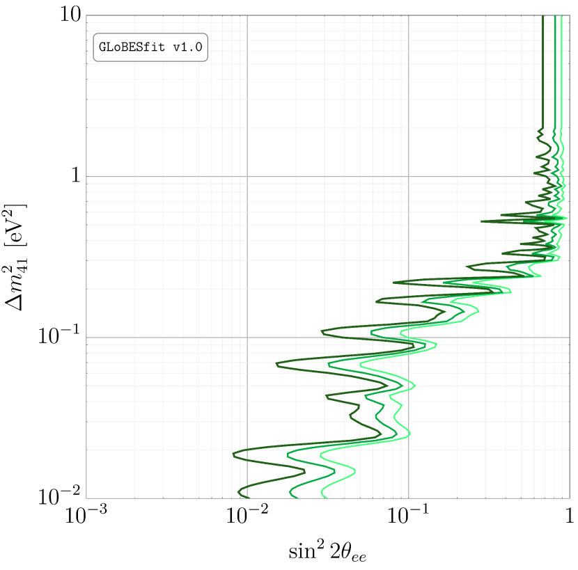
Once more, we employ a chi-squared function of the form
| (V.13) |
where and are the experimental and predicted IBD spectra, respectively. We reweight the measured data by a factor of
to ensure consistency in our GLoBES analysis. The covariance matrix includes the statistical and systematic uncertainties described above, neglecting the energy scale uncertainty, including correlations.
The nuisance parameter describes adjustments to the energy scale at RENO, accounting for its uncertainty . The effect of the energy scale shift is included through the GLoBES function glbShiftEnergyScale. In our calculations, we minimize with respect to this nuisance parameter for every point in the – plane.
In an attempt to faithfully reproduce this experiment in GLoBES, we reweight our predicted spectrum by an ad hoc factor , determined as follows. We have simulated the IBD spectra at RENO assuming the best-fit value of determined in Ref. Bak et al. (2018), i.e., = 0.0896. We then replace , and minimize over . We find the minimum at . We then use this value of in all subsequent calculations.
VI Spectral Analyses
In this section, we present and discuss our analyses of the experiments presented in the previous section. In particular, we consider several groupings of these experiments and assess the significance of the evidence for the existence of a sterile neutrino.
VI.1 Aggregating Results
In Table 9, we combine relevant statistical quantities from our sterile-neutrino analyses of the experiments described in Sec. V. We also tabulate the locations of the best-fit points in the – plane for each experiment; these suppressed in Figs. 26-31 for clarity.
| Experiment(s) | Best-Fit Point, | |||||
|---|---|---|---|---|---|---|
| Bugey-3 | 12.6 | 25 | 9.2 | 0.17 | 01.4 | (, ) |
| DANSS | 33.5 | 24 | 21.3 | 3.0 | (, ) | |
| Daya Bay | 45.0 | 52 | 42.7 | 0.33 | 0.98 | (, ) |
| Double Chooz | 8.0 | 26 | 5.7 | 0.31 | 1.0 | (, ) |
| NEOS | 65.4 | 60 | 54.1 | 2.9 | (, ) | |
| RENO | 23.6 | 25 | 19.7 | 0.15 | 1.5 | (, ) |
| DANSS + NEOS | 98.9 | 84 | 84.9 | 3.3 | (, ) | |
| Daya Bay + NEOS | 110.4 | 112 | 103.6 | 2.1 | (, ) | |
| Total | 188.2 | 212 | 175.2 | 3.2 | (, ) | |
| Modern | 175.5 | 187 | 161.7 | 3.3 | (, ) |
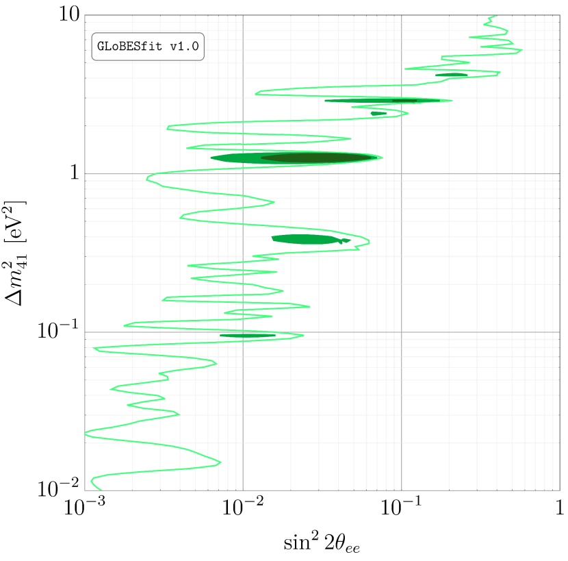
VI.2 Combined Sterile Neutrino Analysis
The exclusion contours from a combined analysis of these spectral measurements is shown in Fig. 32. Since we have assumed correlations between these experiments are small, this figure is equivalent to the naive additional of the maps in Figs. 27-30. Relevant statistics are compiled in the penultimate line of Table 9. At the best-fit point, we find ; given the three-neutrino value , this corresponds to , or roughly .
While introducing a sterile neutrino has significantly improved the fit, the three-neutrino hypothesis is not obviously insufficient — for 212 degrees of freedom, the above value of corresponds to . All of Bugey-3, Daya Bay, Double Chooz and RENO have values of that are less than the number of data points used in each analysis; simply put, these experiments do not convey a need to introduce a sterile neutrino. On the other hand, DANSS and NEOS show a strong preference for a sterile neutrino, as previously discussed (particularly the former); these experiments drive the global preference for a sterile neutrino, as has been previously observed Dentler et al. (2017, 2018); Gariazzo et al. (2018). The best-fit point in Fig. 32 is at , which is roughly consistent with the best-fit point from the spectral analyses in Refs. Gariazzo et al. (2018); Dentler et al. (2018).
VI.3 Additional Analyses
In this subsection, we discuss particularly interesting subsets of the spectral-ratio data and the extent to which these indicate the possible existence of a sterile neutrino.
Calibration: Measuring and
We begin this section by discussing how we verify that our GLoBES analyses of Daya Bay, Double Chooz and RENO reproduce the experimental measurements of the three-neutrino parameters and in the absence of a sterile neutrino. We scan over these parameters and calculate the precisely as described above; the results are shown in Fig. 33. The dark (light) regions represent the 95% (99%) C.L. contours derived for each of Daya Bay (red), Double Chooz (purple) and RENO (blue). The gray curves represent a combined analysis of all three of these.
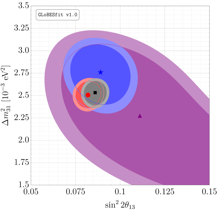
These regions are broadly consistent with the best-fit values found in the analyses of the respective collaborations Adey et al. (2018); Bak et al. (2018); De Kerret et al. (2019).141414We elect to frame this analysis in terms of instead of . The precise relationship between these two quantities has been debated in the literature Parke and Zukanovich-Funchal (2019); Adey et al. (2019c), but this is not relevant for our purposes here. This figure can also be compared against Fig. 5 of Ref. Esteban et al. (2019), where a combined analysis of these medium-baseline experiments has also been performed. We again find general agreement between the calculated regions. The correspondence is not exact – for instance, the region preferred by Double Chooz is slightly wider here than the corresponding region in Ref. Esteban et al. (2019) – but given that these fits have been performed with often incompletely reported information, we consider this a modest success.
One may worry that introducing a sterile neutrino may cause a significant mismeasurement of at reactor experiments. We have investigated how sensitivity to a sterile neutrino changes if is unfixed from its best-fit value, and how introducing a sterile neutrino may shift the preferred value of .151515Given that accelerator neutrino experiments also provide a measurement of , and that these measurements are consistent with the value measured at reactors, we leave this parameter fixed at its best-fit value for this study. We find, however, that this is not the case. The measurement of is driven primarily by Daya Bay (see Fig. 33), whereas the measurement of is driven primarily by DANSS, and that these measurements are largely uncoupled when performed simultaneously. This validates our fixing in our analyses above.
DANSS and NEOS
Given that DANSS and NEOS drive the sensitivity to a sterile neutrino in our global fit, it seems pertinent to ask how the combination of just these two experiments constrains the – plane. The resulting 95%, 99% and 99.9% C.L. contours are shown in dark green, green and light green, respectively, in Fig. 34. Relevant statistics are compiled in Table 9 in the row headed “DANSS + NEOS.”
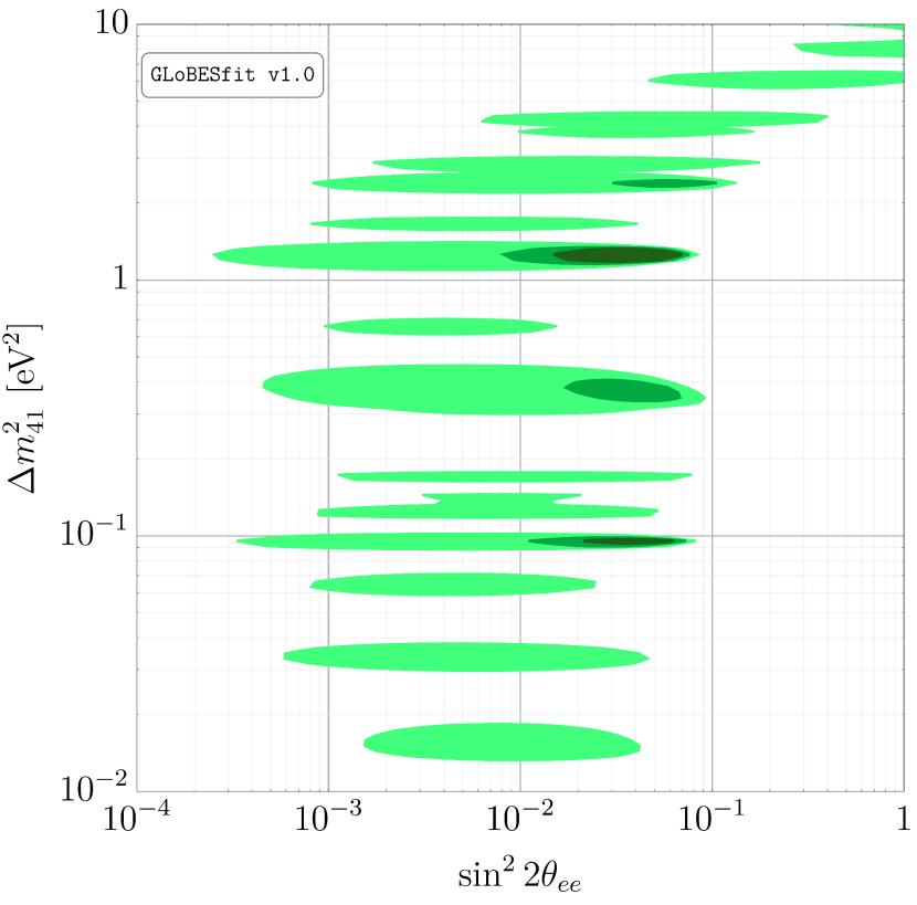
Restricting to these two experiments has resulted in , corresponding to . Notice, however, that the value of the chi-squared at the best-fit point, , is 84.9. For 82 degrees of freedom, this corresponds to ; this is an acceptable fit, but hardly compelling evidence for the existence of a sterile neutrino. Moreover, the best-fit points from our analyses of DANSS and NEOS do not coincide, and the best-fit point from their combination lies close to that from DANSS alone. Consequently, we have investigated the compatibility of these data sets using a parameter goodness-of-fit test Maltoni and Schwetz (2003). We define
| (VI.1) |
where is the minimum value of the chi-squared for experiment . We find ; assuming this is chi-squared distributed implies . These data sets seem to be in mild tension. While parameter goodness-of-fit values should be viewed with some skepticism (see, for instance, Ref. Diaz et al. (2019)), it bears mentioning that the evidence for a sterile neutrino from this experiments, while modestly strong, is not entirely overwhelming.
Daya Bay and NEOS
Given the manner in which we have been forced to include NEOS – namely, as a ratio with respect to Daya Bay’s EH1 – one could reasonably object that showing results from NEOS on its own has stripped this analysis of valuable context. To this end, we have performed a combined analysis of Daya Bay and NEOS, the results of which we show in Fig. 35. The resulting 95%, 99% and 99.9% C.L. contours are shown in dark green, green and light green, respectively, and relevant statistics are compiled in Table 9 in the row headed “Daya Bay + NEOS.”
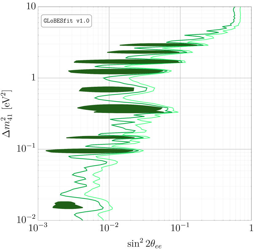
While the best-fit point to the NEOS data unto itself lies in the region around eV2, this part of the parameter space is disfavored by the medium-baseline experiments, including Daya Bay. Combining Daya Bay and NEOS makes this apparent; while this part of the parameter space is still allowed, much more of the sterile neutrino parameter space is included in the at 95% C.L. region.
As mentioned in Sec. V, we have ignored possible correlations between Daya Bay and NEOS in our analysis because they are hard to quantify exactly. Consequently, this analysis is tantamount to adding together the individual maps over the sterile neutrino parameter space. We note, however, that accounting for these correlations is one way in which this analysis can be strengthened in the futurel e look forward to improving this treatment in future versions of GLoBESfit.
Analyzing Modern Experiments
In our analyses of rate experiments, we considered how considering only experiments from the 2010s alters the evidence for a sterile neutrino. In the interest of parity, we perform a similar analysis here. For the experiments that we consider, this is tantamount to removing Bugey-3 from the fit.
We show the results of this analysis in Fig. 36. As before, the 95%, 99% and 99.9% C.L. contours are shown in dark green, green and light green, respectively. Relevant statistics are compiled in the last line of Table 9. It is clear that removing Bugey-3 from the fit has not dramatically changed the best-fit region (cf. the dark green region in Fig. 32). In fact, the fit is slightly stronger for Bugey-3’s omission — the preference for a sterile neutrino rises to which, while not much higher than , is an increase relative to the analysis of all experiments. The reason for this is clear from Fig. 26: Bugey-3 indicates no preference for a sterile neutrino at eV2. In fact, our analysis implies that the best-fit point from our analysis of modern experiments is less favored than zero mixing by the Bugey-3 data.
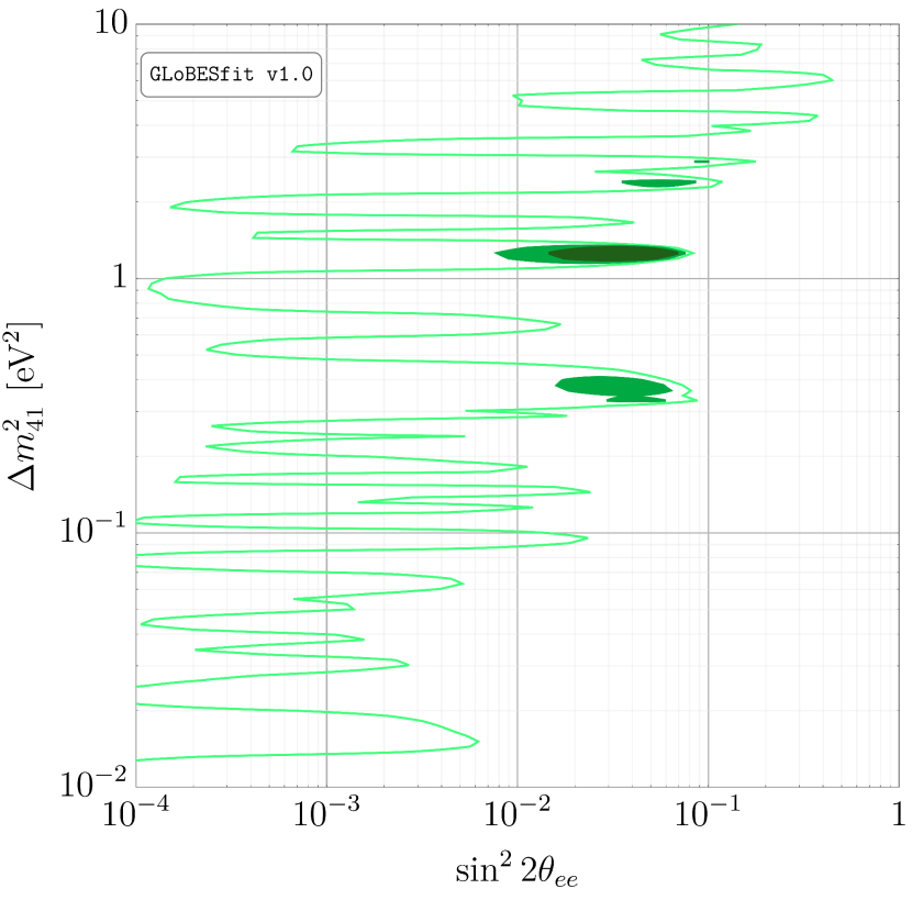
We emphasize that we know of no concrete reason why any experiment performed before 2010 (in this case, Bugey-3) should be disregarded in any of the fits we have performed. We mean merely to demonstrate that if one were suspicious of these data, for whatever reason, then their inclusion has not dramatically enhanced the preference for a sterile neutrino – the evidence is, in fact, largely driven by experiments from the past decade.
Energy Scale Uncertainties at Bugey-3, DANSS and NEOS
An important source of systematic uncertainty in these experiments is the energy scale of the detector. While the energy scale of liquid scintillator detectors is nonlinear, we assume in our analyses that the energy response is linear, and that the only uncertainty is on the slope of this energy response. This is precisely the meaning of the nuisance parameters in Sec. V.
Loosely speaking, the uncertainty on the energy scale translates into uncertainty on the inferred value of ; a systematic shift in reconstructed values of induces a corresponding offset in the measured value of . If the energy scales were changed at these experiments, then the fringe-like structures in the resulting confidence level contours would similarly be shifted up and down in Figs. 26-31.
As we have discussed, the evidence for a sterile neutrino is driven by the combination of DANSS and NEOS. This can be seen from Figs. 27 and 30 by looking at the fringes in the confidence level contours: the best-fit point resides in the region where the patterns of fringes line up and leave a gap in the sterile neutrino parameter space. One could then ask if the patterns of fringes can be moved relative to one another to produce an allowed region elsewhere. Conversely, we have also seen that Bugey-3 presents a mild challenge to the sterile-neutrino interpretation of modern spectral experiments. One could also ask if allowing the energy scale to vary at Bugey-3 allows for this tension to be mitigated.
Unsurprisingly, we find that shifting the energy scales within their stated error budgets does negligibly little to address either of these concerns – clearly, this would have already appeared in our analyses, wherein the energy scales are allowed to vary as nuisance parameters. One could, however, ask how increasing these uncertainties modifies our analyses. We have repeated these analyses with the energy scale uncertainties all increased to 20%.161616We do not claim that any of these experiments has underreported their energy scale uncertainty. We mean merely to isolate the effect of this particular contribution to the overall error budget. Even here, we find that the resulting patterns of fringes have not appreciably moved in the direction relative to the nominal analyses. Therefore, we are led to conclude that energy scale uncertainties do not contribute meaningfully to the preference for a sterile neutrino in these experiments.
VII Sterile Neutrinos and the 5 MeV Bump
The presence of an unexplained spectral feature at 5.0 MeV in the absolute prompt energy spectrum, independently observed by several experiments Choi et al. (2016); An et al. (2016); Abe et al. (2016), has caused significant interest in recent years. In a sense, the so-called 5 MeV bump is a microcosm of the current situation regarding reactor antineutrino anomalies: there is a lingering suspicion that some unaccounted-for nuclear physics effect is operative, but precisely how this filters into the hunt for sterile neutrinos is unclear. In Ref. Berryman et al. (2019), it was proposed that the bump could arise from the process 13CC in the presence of some new interaction. While this interaction could, in principle, explain the excess, it was found that concrete models of potential new physics that could provide such an interaction are already strongly constrained. This all suggests that nuclear physics effects are a much more likely explanation of the bump.
Still, if the bump is indeed the result of a misunderstanding of the antineutrino flux, then this does not imply that a sterile neutrino does not exist. However, it is important to understand the effect that the bump has on searches for sterile neutrinos; this is the subject of this section. In the first subsection, we study a subset of the global dataset indicating the existence of the bump to determine how strong the evidence for this bump is. In the second, we present sterile neutrino analyses of the global reactor dataset with a phenomenological parametrization of the bump, and discuss the results.
VII.1 The Evidence for the Bump
We begin by considering the most relevant subset of the evidence for the existence of the bump. In particular, we consider the following three measurements:
-
1.
The measurements of the isotopic prompt energy spectra for 235U and 239Pu inferred from Daya Bay burn-up measurements in Ref. Adey et al. (2019a). We ignore the first three and the last two bins for each of these spectra, where experimental systematic uncertainties can be large.
-
2.
The fractional excess of events in the region [3.8, 7.0] MeV (prompt energy) relative to the HM flux predictions, published by RENO in Fig. 5 of Ref. Bak et al. (2019).
-
3.
The 235U spectrum measured by PROSPECT in Ref. Ashenfelter et al. (2019).171717While we have included PROSPECT as a part of this analysis, we reiterate that we do not include this experiment as a part of our sterile neutrino exclusion.
We make extensive use of the supplementary material published by the Daya Bay and PROSPECT collaborations, as pertains to these measurements. For the RENO data, we have digitized Fig. 5 of Ref. Bak et al. (2019) for our analysis. More specifically, Daya Bay and PROSPECT have published covariance matrices for their measured spectra, including nontrivial correlations; for RENO, we assume that the data are uncorrelated in the absence of concrete information.
We ask how well these data are described by the HM fluxes and determine the extent to which introducing a bump affects the quality of this fit. To these ends, we use the Markov Chain Monte Carlo (MCMC) package emcee Foreman-Mackey et al. (2013) to perform two types of analyses. In the first, we allow only the magnitudes of the isotopic fluxes of 235U and 239Pu to vary – multiplied by quantities and , respectively – while maintaining the shapes given by the HM fluxes. In the second, we add a separate Gaussian feature to each of these isotopic fluxes. The Gaussians themselves are normalized to unit area, though we multiply them by and , respectively; we simplify our analysis by fixing the means of these Gaussians to 5.8 MeV antineutrino energy (corresponding to 5.0 MeV prompt energy), and we assume they share a common width . We scan over the appropriate parameter spaces and determine the posterior probability densities for each case, and compare the maximum likelihoods.
We have considered two combinations of the data mentioned above. For the first, we simultaneously analyze Daya Bay and RENO; for the second, we add PROSPECT into the analysis. The PROSPECT spectrum of Ref. Ashenfelter et al. (2019) has been presented with arbitrary normalization. To account for this, we introduce a free-floating parameter to rescale the predicted 235U spectrum at PROSPECT, independent of above. Table 11 shows relevant statistics from our analysis performed in the absence of a bump. We present the maximum value of the likelihood in terms of the minimum value of . Shown also are the number of degrees of freedom , and the -value derived assuming is Gaussian-distributed. Moreover, Table 11 shows the same quantities for our analyses in which bumps in the isotopic fluxes are introduced. Clearly, the current data greatly prefer this sort of bump over the pure HM fluxes.
| Analysis | |||
|---|---|---|---|
| Daya Bay + RENO | 172.3 | 40 | |
| ” + PROSPECT | 212.2 | 71 |
| Analysis | |||
|---|---|---|---|
| Daya Bay + RENO | 32.0 | 37 | 0.70 |
| ” + PROSPECT | 91.8 | 68 |
More of the structure of the fits in which a bump is invoked is shown in Figs. 40 and 41 in Appendix C for our analyses without and with PROSPECT, respectively. In the two-dimensional planes, the blue, orange and red contours represent the 68.3%, 95% and 99% credible regions (C.R.), respectively. Additionally, the one-dimensional plots also show the 90% C.R. curve in green. Firstly, both analyses prefer the HM fluxes to be rescaled downward in magnitude, particularly for . Secondly, while the data are largely consistent with the absence of a bump in 239Pu, nonzero is preferred at — the data unequivocally prefer a spectral distortion.
The fit to Daya Bay and RENO in the presence of a bump is fairly high quality () but degrades quite steeply () when PROSPECT is introduced. The reason is straightforward. The Daya Bay and RENO analyses prefer for the absolute IBD yields from 235U to be scaled down by %.181818The best-fit rescaling of the Daya Bay 235U flux that we calculate here () is smaller than that published by the collaboration (0.92) Adey et al. (2019a). Daya Bay has determined this value by fitting to the total number of events, whereas we have fit based on the measured spectrum; the systematics associated with these measurements differ, so one would not necessarily expect these procedures to yield the same result. This primarily stems from the deficit of events observed at low energies at Daya Bay, whereas the spectrum above MeV is largely consistent with the HM prediction (see Fig. 1(a)). On the other hand, the PROSPECT spectrum is reasonably consistent with the shape of the HM prediction for the 235U flux, to within modest-sized uncertainties, over the entire energy range, particularly in the low-energy region. Clearly, the fit cannot successfully reconcile these differing low-energy behaviors. The issue of the reactor bump may be a commentary on the low-energy spectrum as much as the high-energy spectrum.
For context, the PROSPECT data, unto themselves, yield ; for , this corresponds to . It bears mentioning that PROSPECT is still collecting data – the discrepancy between the PROSPECT and Daya Bay measured 235U spectra may well be resolved with increased statistics and improved analysis techniques.
VII.2 Sterile Neutrino Analyses with the Bump
We turn now to the issue of how the inclusion of a bump in the isotopic flux of 235U alters the evidence for the existence of a sterile neutrino. We will consider both rate and spectral analyses in turn.
We begin by considering the effect of the 5 MeV bump on our rate analyses in Secs. III and IV. Antineutrinos in the range [5.3, 6.3] MeV are predicted to constitute 13.5% of IBD events at these experiments. If the 235U flux is augmented with a Gaussian bump of the sort indicated by our Daya Bay/RENO/PROSPECT analysis, i.e, a Gaussian bump with height (cf. Fig. 41), then this factor becomes 14.4% — a 0.9% increase. Moreover, since many of the experiments considered here have fission fractions of the order , we see that adding this sort of Gaussian bump increases the predicted IBD rate by %. This will not be enough to explain the entire deficit with respect to the HM prediction, as we will see.
On the other hand, we have the measurements of ratios of spectra in Secs. V and VI. As argued previously, we expect these measurements to be largely insensitive to the details of the antineutrinos flux. Therefore, we do not expect the 5 MeV bump to significantly affect searches for sterile neutrinos in this channel, either.
We have confirmed this suspicion by calculating the distribution of over the – plane – precisely as has been done previously – with the additional contribution from a Gaussian bump in 235U. We vary the height of the bump between and in the units of Figs. 40 and 41, and have determined that the minimum value of the changes by less than one unit over this range. Specifically, we find 191919This does not agree with the equivalent value in Table 9 because we are using the HM fluxes as our baseline here, whereas before we had been using the ab initio fluxes. and . The bulk of this difference is attributable to NEOS, given their unconventional approach to normalizing their spectrum. Moreover, we find that the statistical significance, in terms of , does not vary meaningfully from .
We are led to conclude that the presence of the 5 MeV bump does not substantively impact searches for sterile neutrinos at reactor experiments, because (1) the contribution of events contained within the bump is at the sub-percent level, and (2) spectral ratios are, by design, largely insensitive to the particulars of the flux model employed.
VIII Regarding Neutrino-4
Neutrino-4 Serebrov et al. (2019); Serebrov is a liquid-scintillator antineutrino detector located at the SM-3 reactor in Dimitrovgrad, Russia. The moveable detector covers a range of distances – between 6 and 12 m – from a 100 MW core. Recently, the collaboration has reported Serebrov et al. (2019) results that imply 3.5 evidence for the existence of a sterile neutrino; preliminary results presented in December 2019 Serebrov suggest that this feature persists with the collection of more data.
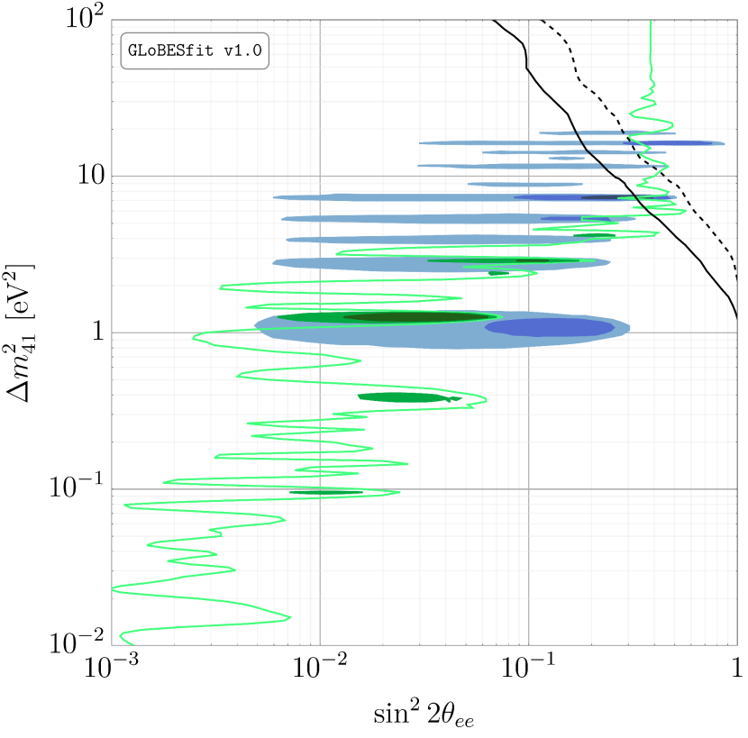
The data currently available to the public are insufficient to allow us to attempt to replicate the collaboration’s analysis. However, we can get a sense for how compatible Neutrino-4 is with the other experiments that we have considered by overlaying their respective allowed contours. We show precisely this in Fig. 37. The dark green, green and light green curves are, respectively the 95%, 99% and 99.9% C.L. contours from our combined analysis of measured spectral ratios from Bugey-3, DANSS, Daya Bay, Double Chooz, NEOS and RENO. The dark blue, blue and light blue curves are the , and allowed contours shown on slide 30 of Ref. Serebrov ; we caution that these results are preliminary, but proceed regardless. We also show the 90% (solid black) and 99% (dashed black) C.L. contours from the combined analysis of the Mainz, Troitsk and KATRIN tritium-endpoint experiments presented in Ref. Giunti et al. (2019b), where a similar comparison has been performed on the basis of Neutrino-4 results from Ref. Serebrov et al. (2019).
As observed in Ref. Giunti et al. (2019b), the best-fit point from Neutrino-4 ( = 0.31, = 7.32 eV2) is disfavored, to a moderate degree, by the tritium-endpoint experiments. Similarly, the best-fit point to Neutrino-4 data is inconsistent with the region preferred by reactor spectral ratios. Moreover, while not shown in Fig. 37, the Neutrino-4 best-fit point is also disfavored by the integrated rate measurements presented in Sec. VI – in particular, see Fig. 22. The degree of (in)compatibility has been tabulated in Table 12. For each of our three rate analyses and for our spectral analysis, we show the difference in between our best-fit point and that of Neutrino-4 (), as well as the corresponding -value and the equivalent number of .
| Analysis | |||
|---|---|---|---|
| Rates + HM | 25.9 | 4.7 | |
| Rates + AI | 63.5 | 7.7 | |
| Rates + HKSS | 17.9 | 3.8 | |
| Spectra | 13.9 | 3.3 |
Clearly, none of the four analyses are particularly tolerant of this result from Neutrino-4. Our spectral analysis disfavors the best-fit point at the level, but all three rate analyses disfavor this point at . It is perhaps imprudent for us to focus solely on the best-fit point from Neutrino-4: significant portions of the -preferred parameter space cannot be firmly refuted by the tritium-endpoint experiments or by our analyses. However, in the absence of enough information to perform our own analysis of Neutrino-4, it is difficult to precisely discuss the global compatibility of these results. Interestingly, the updated analysis of Ref. Serebrov contains a -preferred region around eV2 that was not present in Ref. Serebrov et al. (2019). If confirmed in an official publication, then this would be broadly consistent with the best-fit region from our analysis of spectral ratios. It is our hope that an extensive data release will allow us to study Neutrino-4 in more depth in the future.
IX Conclusions
In this work, we have studied the evidence for the existence of sterile neutrinos contained in the global reactor antineutrino dataset using a new open-source, GLoBES-based toolkit that we call GLoBESfit. We have demonstrated that inferences from IBD rate measurements are confounded by the necessary dependence on a particular flux model. In particular, while the evidence obtained using the traditional HM fluxes is at the level of , updated ab initio fluxes imply significance, while updated spectral-conversion fluxes yield significance. This discrepancy can only be resolved with continued improvements to predictions of reactor antineutrino fluxes, which in turn rely on the collection of improved data. Ratios of measured IBD spectral, on the other hand, seem to paint a more optimistic picture: taken together, the current dataset suggests that the evidence rises to the level of . This is certainly tantalizing, but is hardly ironclad. Therefore, we are led to conclude that that issue of the existence of additional species of neutrinos cannot be resolved one way or another with current data. We have also addressed the 5 MeV bump, and have found that the presence of this feature does not dramatically alter inferences about sterile neutrinos.
In addition to presenting our results, this manuscript is also intended to document GLoBESfit. This software is available for download from either GitHub Berryman or from our dedicated website Berryman and Huber . The function of making GLoBESfit publicly available is twofold:
-
1.
Publishing our code allows for members of the community to levy informed commentary on our techniques. Global fitting in an inherently tricky business; reproducing an experiment’s results can be challenging for those not involved in the collaboration. Invariably, there are aspects of this program that can be improved. Our hope is that public input, over time, will reinforce this work.
-
2.
Though we intend to revisit and expand on this work in the future, it is not possible for us to test every interesting physical hypothesis that could explain current neutrino anomalies. We have focused on the 3+1 scenario because of its simplicity, but Nature could certainly be far more interesting than this. If a user is interested in testing a particular model, then the tools we have developed ought to allow them to at least start that process. Because GLoBESfit is developed using pre-existing GLoBES architecture, it should lend itself to much a wider set of applications than the relatively simple scenario we have considered here.
Our hope is that making these tools available contributes meaningfully to the wider neutrino physics community.
Regarding The Use of Statistics
A common sin in global analyses is assuming that is chi-squared distributed. This issue has been discussed in detail in the literature; see, for instance, Refs. Feldman and Cousins (1998); Agostini and Neumair (2019); Silaeva and Sinev (2020). Analyses of spectral ratios are particularly susceptible to this statistical idiosyncrasy, as is demonstrated nicely in Fig. 5 of Ref. Agostini and Neumair (2019); we direct the interested reader to this work for more details. The primary issue is that while the expected ratio of spectra is flat in the absence of a sterile neutrino, statistical noise invariably results in a preference for oscillations with some nonzero amplitude. Failing to take this into account yields final results that are overconfident. In this work, we have been conservative in talking about the statistical significance of our findings, particularly those in Sec. VI. While the significance we have presented here ostensibly rises to the level, the true significance is certainly less than this. The actual preference for a sterile neutrino in the global reactor dataset, accounting for this effect, remains to be determined.
The difficulty is that the precise relationship between and a -value depends strongly on the experiment(s) under consideration. How is distributed – and thus the -value associated with a particular measurement – can be determined numerically as a function of and using Bayesian methods; this is the basis of the Feldman-Cousins technique Feldman and Cousins (1998). However, this requires the ability to reliably simulate the experiment(s) under consideration; the capacity to do so is limited for those not involved in a given collaboration. Even with perfect simulation capabilities, however, this sort of analysis can be prohibitively computationally demanding, particularly if considering multiple experiments simultaneously. We hope to address these concerns in future releases of GLoBESfit, but for the time being, we are left wanting for a more sophisticated statistical treatment.202020As this work neared completion, Ref. Giunti (2020) appeared on the preprint arXiv. In this work, the author performs precisely the sort of analysis advocated above. They find that such a Feldman-Cousins correction diminishes the overall significance from to . We note that the author has included data from PROSPECT Ashenfelter et al. (2018), as well as preliminary, updated data from DANSS Danilov (2019), but not from Daya Bay, Double Chooz nor RENO; this explains the difference in significance relative to our findings here.
While we believe that the results we have presented here are merited in their own right, our hope is that presenting the results as we have – and acknowledging the ways in which the underlying treatment is deficient – is sufficient to promote dialogue between experimentalists and theorists on how to best employ the available data. It is incumbent on theorists to ensure that experimental data is used correctly in their analyses; it is incumbent on experimentalists to follow good data preservation practices. Decisions for how to best commit the neutrino community’s finite resources ultimately rely on understanding what is (and is not) contained in current data.
Acknowledgments: We thank Pedro Ochoa-Ricoux and Liang Zhan (Daya Bay); Giorgio Gratta (Palo Verde); Karsten Heeger, Bryce Littlejohn and Pranava Teja Surukuchi (PROSPECT); Soo-Bong Kim (RENO); and David Lhuillier (STEREO) for providing data and useful discussions. We further thank Muriel Fallot for providing the ab initio fluxes in machine-readable format and Leendert Hayen for information on the HKSS model, as well as Carlo Giunti and Marco Laveder for discussions regarding Neutrino-4. JMB thanks the Fermilab Neutrino Physics Center for their hospitality during the completion of this work, as well as André de Gouvêa, Peter Denton, Kevin Kelly and Yue Zhang for helpful conversations. We again thank Bryce Littlejohn for pointing out bugs in a previous version of this analysis. This work is supported by DOE Office of Science awards DE-SC0018327 and DE-SC0020262. The work of JMB is also supported by NSF Grant PHY-1630782 and by Heising-Simons Foundation Grant 2017-228.
Appendix A Sterile Neutrinos in GLoBES
In this appendix, we outline how oscillations involving sterile neutrinos are calculated using existing GLoBES machinery. We begin by reviewing the basics of oscillations with sterile neutrinos before turning to our implementation thereof. We stress that this machinery can be modified to implement any new-physics scenario that the user wishes to probe; our discussion of how to create custom oscillation engines and probability matrices is completely generalizable.
A.1 Oscillations with a Sterile Neutrino
The generic expression for the vacuum oscillation probability – the probability for a neutrino produced in the flavor eigenstate to be observed in the flavor eigenstate () – is given as follows:
| (A.1) | ||||
where (; ) are the elements of the leptonic mixing matrix, is the distance propagated (i.e., the baseline), is the neutrino energy and we define , with the neutrino masses. For oscillations involving antineutrinos, we make the replacement ; this is equivalent to changing the sign of the last term in Eq. (A.1).
There are only four relevant elements of the leptonic mixing matrix, for our purposes here. We parametrize them as follows:
| (A.2) | ||||
| (A.3) | ||||
| (A.4) | ||||
| (A.5) |
one can easily verify the unitarity constraint . In our analyses, we have assumed that the values of and determined from global fits to oscillation data assuming three-neutrino oscillations Esteban et al. (2019) can be applied without alteration. Of course, what experiments actually measure is (some combinations of) the elements of the leptonic mixing matrix. Consequently, a determination of, say, is absolute, whereas the inferred value of will depend on values of and inferred elsewhere. However, as long as is small – which we find to be the case in our fits – the implied modifications to the three-neutrino mixing angles are also small.
When (anti)neutrinos propagate through matter, the background potential from ambient protons, neutrons and electrons modifies their propagation. The effects of this matter potential can be included via modifications to the mixing angles and mass-squared differences. Moreover, GLoBES does contain the functionality to calculate neutrino propagation in a matter background. Given the low energies under consideration here, however, we assume that the vacuum-oscillation formalism is sufficient.
For short-baseline experiments – experiments with baselines m – with point-like sources and a point-like detectors, we use the two-flavor approximation for the electron-type survival probability, :
| (A.6) |
where is the effective active-sterile mixing angle. We work in terms of even though this is equal to in our parametrization; the effective angle is parameterization independent and thus more appropriate for comparison with the broader literature.
For medium-baseline experiments, this two-flavor formalism is insufficient — we consider the full, four-flavor formalism. The electron-type survival probability is instead written as
| (A.7) |
this can be immediately derived from Eq. (A.1) by setting .
For the experiments we consider, we often cannot consider oscillations with one well-defined baseline: either (1) the experiment is sourced by multiple reactors, or (2) the physical extent of the core or detector (or both) is not much smaller than the distance between them. In either case, one must generalize the term to a flux-weighted average over baselines. The appropriate quantity is
| (A.8) |
where we define and introduce as the distribution of baselines in the experiment. The denominator is the mean-inverse-squared baseline, which we denote . We discuss our implementation of these integrals below.
A.2 Implementation in GLoBESfit
The survival probability is calculated in GLoBES with custom oscillation engines using the function glbDefineOscEngine, which is called in the main program file. A sample call of this has the following form:
glbDefineOscEngine(NUMP,
&<exp>_probability_matrix,
&glf_get_oscillation_parameters,
&glf_set_oscillation_parameters,
‘‘<engine_name>’’, user_data);
We explain the arguments of this function below.
NUMP: The maximum number of oscillation parameters used. For four-neutrino oscillations, this number should be 12; practically, we take it to be 6.
<exp>_probability_matrix: This is the function in which the oscillation probabilities are calculated for experiment <exp>. This function produces a three-by-three matrix P whose elements are the active-active oscillation probabilities (i.e., P[0][0] corresponds to , P[0][1] to , etc.). Currently, these functions only calculate ; all other probabilities are fixed to 0. We discuss the evaluation of the probabilities in the next subsection.
glf_get_oscillation_parameters: This function retrieves the current values of the oscillation parameters.
glf_set_oscillation_parameters: This function sets the values of the oscillation parameters.
‘‘<engine_name>’’: This is the internal name of the oscillation engine, which is called in the corresponding AEDL file via $oscillation_engine=‘‘<engine_name>’’.
user_data: A void pointer to user-specified data that are relevant for the evaluation of the probability. We discuss the use of this apparatus below.
A.3 Custom Probability Matrices
For most of the experiments we consider, it is sufficient to take the core to be point-like but to give the detector finite extent. We usually make the approximation that the detector constitutes a (portion of a) spherical shell centered around the core. The function is then flat over the extent of the detector, which we consider to be ; this leads to a relatively simple expression for ,
| (A.9) |
as well as the function in Eq. (A.8):
| (A.10) | ||||
where is the sine integral.
For each experiment of this sort, the width of the detector is specified in GLoBESfit as the sole element of an array typically named <exp>_wide. This is passed into the probability engine by setting “user_data” to be “(void *) <exp>_wide” in glbDefineOscEngine, above. The function in Eq. (A.10) is evaluated, using this input, with a helper function called lsin(q, La, Lb). Here, La and Lb are the nearest and further baseline at the experiment, determined from the width and the (average) baseline thereof. Note that all lengths in GLoBES are assumed to be in km. Moreover, since GLoBES also assumes all energies are in GeV, in this function is numerically given by
| (A.11) |
Occasionally, the experimental geometry results in a more complicated whose structure we must take into account. This distribution is estimated using a simple Monte Carlo routine. Pairs of points are randomly drawn from the core and detector, whose geometry we must specify by hand. One can then numerically integrate over this distribution to determine and ; this numerical integral is performed as a sum over these pairs.
To save computation time, is precomputed on a grid and is fed into GLoBESfit as a look-up table, whose elements are of the form { log_10 q, F(q)}, that resides in auxiliary header files. Linear interpolation in log_10 q is used to get intermediate values. If is less than some minimum specified value , then it is assumed that the integral scales quadratically and is determined by extrapolation. If is instead greater than some maximum specified value , then it is assumed that has averaged out to 0.5. The values of and depend on the experiment under consideration. We adopt this method for Daya Bay and RENO for both the rate and spectral analyses; moreover, we do this for Bugey-3,212121We do not use this technique for Bugey-3 or Bugey-4 for the rate-only analysis because we expect the antineutrino spectrum to be more sensitive to the specific experimental geometry than the total event rate. DANSS, Double Chooz and NEOS for our spectral analysis.
The precomputed is fed into the custom oscillation engine via the “user_data” option. This is handled by a custom data structure called “glf_distance_data”, whose elements are the length of the precomputed array and a pointer to the array itself. The structure for experiment <exp> is named “<exp>_s”; this is handled by by setting “user_data” to be “(void *) &<exp>_s” in the definition of the oscillation engine.
For medium-baseline experiments, each detector and reactor can be considered point-like, but these experiments are sourced by multiple reactors. The reactors generically have different average powers over the duration of the experiment; these weight their contributions. The integrals over baselines in and are replaced by sums:
| (A.12) | ||||
| (A.13) |
where indexes the reactors, of which there are , and the average power of each is .
For rate-only analyses, the multiple reactors at Chooz, Double Chooz and Palo Verde are handled using different AEDL experiment definitions; the resulting event rates are added at the analysis level. Meanwhile, for rate-only analyses of Daya Bay and RENO, as well as the spectral analyses at Daya Bay, Double Chooz and RENO, the contributions of multiple reactors are combined at the level of the AEDL file. This is purely a function of the development history of GLoBESfit and does not reflect differing physics in these cases.
Appendix B Structure of the Code
In this appendix, we document the component files of GLoBESfit and briefly describe the function and contents of each.
B.1 Common Files
We begin with files that are common to both the rate and spectral modules.
Pure_<isotope>.dat: The antineutrino fluxes for isotope <isotope> = U235, U238, Pu239, Pu241, written in the standard GLoBES format. These fluxes have been calculated from the Huber-Mueller (HM) predictions, linearly interpolated/extrapolated on a logarithmic scale (i.e., the logarithm of the flux has been linearly interpolated/extrapolated).
Pure_<isotope>_SM.dat: Antineutrino fluxes similar to Pure_<isotope>.dat, except that the HM fluxes have been replaced in favor of the ab initio fluxes. (Note that “SM” in the file name stands for “summation method,” which is an alternate name for the ab initio method.)
Pure_<isotope>_HKSS.dat: Antineutrino fluxes similar to Pure_<isotope>.dat, except that the HM fluxes have been replaced in favor of the HKSS fluxes.
IBDnew.dat: The IBD cross section calculated from the results of Ref. Vogel and Beacom (1999) (i.e., Eqs. (14) and (15) of that reference). This is the cross section calculation used in the analyses presented here.
glf_precomputed_probabilities.h: An auxiliary file that contains the look-up tables used to compute for Daya Bay, RENO, DANSS, Double Chooz, NEOS and Bugey. This is called by both glf_rate.c and glf_spectrum.c (see below).
glf_probability.c: A file that contains helper functions and probability engines (see Appendix A) for both the rate and spectral analysis. This file contains generic oscillation engines for point-like reactor cores and detectors of finite extent for both two-flavor (glf_probability_matrix) and four-flavor (glf_standard_probability_matrix) oscillations. Moreover, for experiments for which oscillation probabilities have been precomputed, there again exist functions for both two-flavor (glf_two_state_probability_matrix) and four-flavor (glf_four_state_probability_matrix) oscillations.
glf_probability.h: The header file associated with glf_probability.c. This is called by both glf_rate.c and glf_spectrum.c.
glf_type.h: The header file wherein the structure “glf_distance_data” is defined. This is called by several files.
Makefile: The file used to make the executables ./glf_rate and ./glf_spectrum (see below). The user may need to modify this file to link to their local GLoBES libraries – specifically, the “prefix” option may need to be set to the location of the user’s GLoBES directory.
B.2 Rate Files
We next consider files specific to the rate module.
rate_combo{2,3}.glb: The files containing the AEDL definitions of the experiments we will consider, described in Sec. III. These files employ the HM flux model. The order of the experiments is important in the evaluation of the chi-squared; we enumerate the experiments contained in each file below.
-
•
Short-baseline experiments are contained in rate_combo.glb:
-
0.
Bugey-4 & Bugey-3, 15 m
-
1.
Rovno 91
-
2.
Bugey-3, 40 m
-
3.
Bugey-3, 95 m
-
4.
Gösgen, 38 m
-
5.
Gösgen, 46 m
-
6.
Gösgen, 65 m
-
7.
ILL
-
8.
Krasnoyarsk 87, 33 m
-
9.
Krasnoyarsk 87, 92 m
-
10.
Krasnoyarsk 94
-
11.
Krasnoyarsk 99
-
12.
Savannah River, 18 m
-
13.
Savannah River, 24 m
-
14.
Rovno 88, All 18 m
-
15.
Rovno 88, 25 m
-
16.
Nucifer
-
0.
-
•
Medium-baseline, total-rate experiments are contained in rate_combo2.glb:
-
17.
Palo Verde, 750 m
-
18.
Palo Verde, 890 m
-
19.
Double Chooz, 355 m
-
20.
Double Chooz, 469 m
-
21.
Chooz, 998 m
-
22.
Chooz, 1115 m
-
17.
-
•
Medium-baseline, fuel-evolution experiments are contained in rate_combo3.glb:
-
23.
Daya Bay, EH1 AD1
-
24.
Daya Bay, EH1 AD2
-
25.
Daya Bay, EH2 AD3
-
26.
Daya Bay, EH2 AD8
-
27.
RENO, Near Detector
-
23.
These numberings correspond to the internal GLoBES ordering. Note that some AEDL files apply to more than one experiment. The ordering of these experiments is a function of the development history of GLoBESfit and is in no way a commentary of any of these experiments.
We define a GLoBES rule for each of the four main, fissile isotopes for each experiment. This allows the user to separate out contribution of each isotope in whatever calculation they are interested in. Moreover, it cuts down on the number of flux files that one must keep on hand; instead of defining a separate flux file for each experiment, one need only combine the fluxes from each isotope with the appropriate fuel fraction. Moreover, the theoretical uncertainties on the isotopic IBD yields for 235U, 238U, 239Pu and 241Pu are declared in the AEDL definition for Bugey-4/Bugey-3 (15 m) in the field @sys_on_errors. We have also made clones of this file that modify how these systematics are treated; see below.
Because the absolute numbers of events are not relevant for our analyses, @time, @power, @norm and $target_mass are all generally set to 1.0 in the AEDL definitions; we comment below on instances in which we deviate from this. The fluxes from each of the four main fissile isotopes for each experiment are considered separately and reweighted by the effective fuel fractions given by each experiment. Consequently, @time, @power and @norm are set to be the same for each component of the flux. The value of $length_tab is set to for each experiment;
Exceptions to this occur for medium-baseline experiments – namely, Palo Verde, Double Chooz, Chooz, Daya Bay and RENO – which are typically sourced by multiple reactors, or are comprised of multiple detectors, whose relative contributions must be taken account.
-
•
For Palo Verde and Chooz, @norm is set equal to the numerical value of the exposure, in GWyr, for each detector, which we have calculated in Sec. III.
-
•
We do something similar for Daya Bay. We set @power equal to the total power delivered to each detector, namely
(B.1) where indexes the eight reactor cores and indexes the periods of operation; the Daya Bay rate-evolution analysis is based on the 1230-day data set from Ref. An et al. (2017c), so we only consider the 6AD and 8 AD periods. We set @norm to be equal to each detectors total efficiency, and $target_mass to be equal to each detector’s mass in tons.
-
•
Since the relative contributions of the reactors used in Double Chooz near detector have not been specified, we assume them to be equal. This allows us to set @norm to 1.0 for each.
rate_combo_no_sys.glb: Similar to rate_combo.glb, except no systematic uncertainties are associated with the HM flux predictions. In this mode, GLoBESfit recycles the AEDL definitions in rate_combo2.glb and rate_combo3.glb.
rate_combo_unfix.glb: Similar to rate_combo.glb, except systematic uncertainties are only applied to 238U and 241Pu. The IBD yields from 235U and 239Pu are left unfixed to allow them to be scanned in our analysis. Note that in this mode, GLoBESfit recycles the AEDL definitions in rate_combo2.glb and rate_combo3.glb.
rate_combo_SM{2,3}.glb: Similar to rate_combo{2,3}.glb, except that the SM fluxes are used in lieu of the HM fluxes.
rate_combo_HKSS{2,3}.glb: Similar to rate_combo{2,3}.glb, except that the HKSS fluxes are used in lieu of the HM fluxes.
glf_rate_aux.h: Experimental inputs for our rate analyses. These include the fuel fractions and experimental IBD rates at each experiment, as well as the (inverses of the) covariance matrices that are used in the determination(s) of the chi-squared function(s). This is called in glf_rate_chi.c.
glf_rate_chi.c: The file containing the chi-squared functions to be used with the GLoBES files described above. There are five such functions – glf_rate_chi_nosys, glf_rate_chi, glf_rate_chi_SM, glf_rate_chi_HKSS and glf_rate_chi_unfix – each to be used in conjunction with a different set of GLoBES files, depending on how the antineutrino flux prediction is to be handled. The default is glf_rate_chi_nosys; we discuss how to change this below.
glf_rate_chi.h: The header file associated with glf_rate_chi.c. This is called in glf_rate.c.
glf_rate.c: The file that gets run by the executable ./glf_rate. The contents are as follows:
-
1.
Code for parsing command-line options. Options are discussed below.
-
2.
Oscillation engine definitions for each experiment.
-
3.
Initialization of the chi-squared functions. The chi-squared function is fed the list of experiments to include in its evaluation though the integer array YesNo.
-
4.
The calculation of the chi-squared. Here, GLoBESfit calculates the chi-squared over ranges of some parameters (described in the main text) and writes the output per the user’s specification. We simulate the rate at each experiment both with (using the GLoBES function glbGetSignalFitRatePtr) and without (glbGetRuleRatePtr) oscillations involving sterile neutrinos and take the ratio of these for each such flux model.
B.3 Spectrum Files
We conclude with files specific to the spectrum module.
spectra{2-6}.glb: The files containing the AEDL definitions. The implementations of these experiments are described in Sec. V; we provide here the internal ordering of experiments, decomposed into host .glb file:
-
•
spectra.glb
-
0.
DANSS, Upper Position
-
1.
DANSS, Lower Position
-
0.
-
•
spectra2.glb
-
2.
Daya Bay, EH1 AD1
-
3.
Daya Bay, EH1 AD2
-
4.
Daya Bay, EH2 AD3
-
5.
Daya Bay, EH2 AD8
-
2.
-
•
spectra3.glb
-
6.
Daya Bay, EH3 AD4
-
7.
Daya Bay, EH3 AD5
-
8.
Daya Bay, EH3 AD6
-
9.
Daya Bay, EH3 AD7
-
10.
NEOS
-
6.
-
•
spectra4.glb
-
11.
Double Chooz, Near Detector
-
12.
Double Chooz, Far Detector
-
11.
-
•
spectra5.glb
-
13.
Bugey-3, 15 m
-
14.
Bugey-3, 40 m
-
13.
-
•
spectra6.glb
-
15.
RENO, Near Detector
-
16.
RENO, Far Detector
-
15.
The indices used here correspond to the internal GLoBES indices for each experiment. As with rate experiments, we define separate GLoBES rules for each of the four main fissile isotopes.
glf_spectrum_aux_1.h: Covariance matrices used in our spectral analyses. This is called in glf_spectrum_chi.c.
glf_spectrum_aux_2.h: Experimental data for our spectral analyses, including the relevant measured spectral ratios and the stated fuel fractions. This is called in glf_spectrum_chi.c.
glf_spectrum_chi.c: The file containing the definition of the chi-squared function(s) detailed in Sec. V.
glf_spectrum_chi.h: The header file corresponding to glf_spectrum_chi.c. This is called by glf_spectrum.c.
glf_spectrum.c: The main file that gets run by the executable ./glf_spectrum. The structure of this file is similar to main_rate.c, above.
B.4 Executables and Options
./glf_rate: The main executable for the rate-only aspect of GLoBESfit.
./glf_spectrum: The main executable for the spectrum aspect of GLoBESfit.
We summarize particularly useful command-line options common to either executable.
-
•
-bN: Allows the user to turn off a particular block of experiments corresponding to the index N. (We call these “blocks” because “experiment” can be ambiguous in the parlance of GLoBES. Removing Daya Bay from the calculation, for instance, requires that we ignore several experiments in the AEDL file.) We comment on these blocks below.
-
•
-rN: Sets the number of points used in each direction in the parameter scan to be N. By default, N = 51.
-
•
-xM,N: Sets the range in direction x, corresponding to to be [M, N]. The default is , .
-
•
-yM,N: Sets the range in direction y, corresponding to to be [M, N]. The default is , .
-
•
-o [file_name] or … > [file_name]: Sets the output file of the parameter scan to be [file_name]. If left blank, then the output is set to stdout, i.e., it writes to screen.
Additionally, there are some options that are specific to the rate-only analysis.
-
•
-S: Turns on systematics stemming from the HM flux predictions. This changes the chi-squared function from glf_rate_chi_nosys to glf_rate_chi.
-
•
-M: Replaces the HM fluxes with the SM fluxes, using the systematic uncertainties of the former. This changes the chi-squared function from glf_rate_chi_nosys to glf_rate_chi_SM.
-
•
-H: Replaces the HM fluxes with the HKSS fluxes, including their own uncertainties. This changes the chi-squared function from glf_rate_chi_nosys to glf_rate_chi_HKSS.
-
•
-u: Turns on systematics stemming from 238U and 241Pu and scans over the normalizations of the 235U and 239Pu fluxes instead of considering a sterile neutrino. This changes the chi-squared function from glf_rate_chi_nosys to glf_rate_chi_unfix.
Note that these options are mutually exclusive and have been listed in order of priority – for instance, entering “-M -S -H” at the command line will be treated as if only “-S” has been entered. There is one further rate-specific option:
-
•
-w: In addition to the values of , and , this option toggles writing the best-fit values of the four nuisance parameters , , and to disk, in that order. This only works in conjunction with -S, -M and -H.
Finally, we list some options that are specific to the spectral-ratio analysis.
-
•
-T: In addition to scanning over and , this option triggers an additional scan over on the range .
-
•
-C: This option eschews the scan over the sterile neutrino parameter space altogether and instead scans over on the range and on the range eV2. (This option has been used to perform the calibration scan whose results are shown in Fig. 33.)
Experimental Blocks
Currently, glf_rate is not set up to isolate every individual experiment. However, given that the covariance matrix decomposes into blocks, this allows us to trivially remove blocks of experiments from the analysis. Most of these blocks consist of only one experiment, while the rest include multiple experiments. Here, we tabulate which experiments correspond to which of these blocks.
-
0.
Bugey-4 + Rovno 91
-
1.
Bugey-3 (15 m+ 40 m + 95 m)
-
2.
Gösgen (38 m + 46 m + 65 m) + ILL
-
3.
Krasnoyarsk 87 (33 m + 92 m)
-
4.
Krasnoyarsk 94
-
5.
Krasnoyarsk 99
-
6.
Savannah River (18 m)
-
7.
Savannah River (24 m)
-
8.
Rovno 88 (1I + 2I + 1S + 2S + 3S)
-
9.
Nucifer
-
10.
Palo Verde (750 m + 890 m)
-
11.
Double Chooz (355 m + 469 m)
-
12.
Chooz (998 m + 1115 m)
-
13.
Daya Bay (EH1 + EH2)
-
14.
RENO
The number associated to each block is the appropriate choice of N to be specified at the command line. As an example, if one wanted to remove Nucifer and RENO from the analysis, one would include “-b9 -b14” at the command line.
glf_spectrum uses similar options for toggling on/off experimental blocks. However, since we treat the six above-mentioned experiments as uncorrelated, each experiment resides in its own block, i.e., there is a one-to-one mapping of experiments to blocks.
Appendix C Supplementary Data
C.1 Data Tables
| D1 | D2 | L1 | L2 | L3 | L4 | |
|---|---|---|---|---|---|---|
| EH1 AD1 | 362.38 | 371.76 | 903.47 | 817.16 | 1353.62 | 1265.32 |
| EH1 AD2 | 357.94 | 368.41 | 903.35 | 816.90 | 1354.23 | 1265.89 |
| EH2 AD3 | 1332.48 | 1358.15 | 467.57 | 489.58 | 557.58 | 499.21 |
| EH2 AD8 | 1337.43 | 1362.88 | 472.97 | 495.35 | 558.71 | 501.07 |
| EH3 AD4 | 1919.63 | 1894.34 | 1533.18 | 1533.63 | 1551.38 | 1524.94 |
| EH3 AD5 | 1917.52 | 1891.98 | 1534.92 | 1535.03 | 1554.77 | 1528.05 |
| EH3 AD6 | 1925.26 | 1899.86 | 1538.93 | 1539.47 | 1556.34 | 1530.08 |
| EH3 AD7 | 1923.15 | 1897.51 | 1540.67 | 1540.87 | 1559.72 | 1533.18 |
| D1 | D2 | L1 | L2 | L3 | L4 | |
|---|---|---|---|---|---|---|
| [GWth] | 2.082 | 2.874 | 2.516 | 2.554 | 2.825 | 1.976 |
| [GWth] | 2.514 | 2.447 | 2.566 | 2.519 | 2.519 | 2.550 |
Tables 13-23 collect some supplementary data that are too cumbersome to have included in the main text of this manuscript.
| EH1 AD1 | EH1 AD2 | EH2 AD3 | EH2 AD8 | EH3 AD4 | EH3 AD5 | EH3 AD6 | EH3 AD7 | |
| Target Mass [ kg] | 19.941 | 19.967 | 19.891 | 19.944 | 19.917 | 19.989 | 19.892 | 19.931 |
| 0.8044 | 0.8013 | 0.8365 | 0.8363 | 0.9587 | 0.9585 | 0.9581 | 0.9588 | |
| [m] | 568.2 | 563.4 | 591.3 | 595.1 | 1633.3 | 1634.6 | 1638.7 | 1639.7 |
| 0.564 | 0.564 | 0.557 | 0.552 | 0.559 | 0.559 | 0.559 | 0.552 | |
| 0.076 | 0.076 | 0.076 | 0.076 | 0.076 | 0.076 | 0.076 | 0.076 | |
| 0.303 | 0.302 | 0.312 | 0.315 | 0.310 | 0.310 | 0.310 | 0.315 | |
| 0.056 | 0.056 | 0.055 | 0.057 | 0.055 | 0.055 | 0.055 | 0.057 |
| Bin | [cm2/fission] | ||||
|---|---|---|---|---|---|
| 1 | 0.5113 | 0.0767 | 0.3445 | 0.0675 | |
| 2 | 0.5279 | 0.0766 | 0.3326 | 0.0629 | |
| 3 | 0.5418 | 0.0764 | 0.3219 | 0.0599 | |
| 4 | 0.5553 | 0.0762 | 0.3113 | 0.0572 | |
| 5 | 0.5699 | 0.0760 | 0.2992 | 0.0549 | |
| 6 | 0.5849 | 0.0758 | 0.2878 | 0.0515 | |
| 7 | 0.6033 | 0.0757 | 0.2744 | 0.0466 | |
| 8 | 0.6304 | 0.0754 | 0.2525 | 0.0417 |
| Fuel Bin, | 0.5113 | 0.5279 | 0.5418 | 0.5553 | 0.5699 | 0.5849 | 0.6033 | 0.6304 |
|---|---|---|---|---|---|---|---|---|
| HM | 0.9430 | 0.9411 | 0.9398 | 0.9387 | 0.9404 | 0.9372 | 0.9361 | 0.9391 |
| Ab Initio | 0.9795 | 0.9786 | 0.9781 | 0.9778 | 0.9804 | 0.9779 | 0.9780 | 0.9827 |
| HKSS | 0.9342 | 0.9323 | 0.9310 | 0.9300 | 0.9316 | 0.9284 | 0.9273 | 0.930 |
| Reactor 1 | Reactor 2 | Reactor 3 | Reactor 4 | Reactor 5 | Reactor 6 | |
|---|---|---|---|---|---|---|
| Near Detector | 660.064 | 444.727 | 301.559 | 339.262 | 519.969 | 746.155 |
| Far Detector | 1563.771 | 1460.826 | 1397.813 | 1380.062 | 1409.389 | 1483.001 |
| Reactor 1 | Reactor 2 | Reactor 3 | Reactor 4 | Reactor 5 | Reactor 6 | |
|---|---|---|---|---|---|---|
| Near Detector | 2.381 | 2.084 | 2.224 | 2.060 | 2.315 | 2.248 |
| Far Detector | 2.363 | 2.082 | 2.144 | 2.111 | 2.387 | 2.319 |
| Operating Time [Days] | [km] | Total Average Power, [GWth] | Efficiency | |
|---|---|---|---|---|
| Near Detector | 1807.88 | 0.4331 | 13.312 | 60.3% |
| Far Detector | 2193.04 | 1.4469 | 13.406 | 68.7% |
| Bin | [cm2/fission] | ||||
|---|---|---|---|---|---|
| 1 | 0.527 | 0.074 | 0.333 | 0.066 | |
| 2 | 0.546 | 0.073 | 0.320 | 0.061 | |
| 3 | 0.557 | 0.075 | 0.310 | 0.058 | |
| 4 | 0.568 | 0.074 | 0.302 | 0.056 | |
| 5 | 0.579 | 0.074 | 0.295 | 0.052 | |
| 6 | 0.588 | 0.075 | 0.286 | 0.051 | |
| 7 | 0.599 | 0.073 | 0.278 | 0.050 | |
| 8 | 0.62 | 0.072 | 0.262 | 0.046 |
| Fuel Bin, | 0.527 | 0.546 | 0.557 | 0.568 | 0.579 | 0.588 | 0.599 | 0.620 |
|---|---|---|---|---|---|---|---|---|
| HM | 0.9348 | 0.9401 | 0.9362 | 0.9327 | 0.9374 | 0.9352 | 0.9364 | 0.9319 |
| Ab Initio | 0.9720 | 0.9787 | 0.9753 | 0.9723 | 0.9780 | 0.9761 | 0.9780 | 0.9746 |
| HKSS | 0.9261 | 0.9313 | 0.9274 | 0.9239 | 0.9286 | 0.9264 | 0.9276 | 0.9231 |
| Reactor 1 | Reactor 2 | Operating Time [Days] | Efficiency | Relative Proton Number | |
|---|---|---|---|---|---|
| Near Detector | 355 m | 469 m | 258.0 | 85.47% | 1.0044 |
| Far Detector | 998 m | 1115 m | 818.0 | 86.78% | 1 |
C.2 Experimental Measurements
We show plots of the ratios of spectra measured at Bugey-3, DANSS, Daya Bay, Double Chooz, NEOS and RENO, which underpin our analyses in Secs. V and VI, in Figs. 38 and 39. The black points and error bars represent the data and their statistical uncertainties. The colored curves represent the expectations assuming three-neutrino oscillations; when relevant, the value of used to calculate the line is the best-fit value as determined by that collaboration. The colored bands represent the total systematic uncertainties, given by the square root of the diagonal elements of the covariance matrix for each experiment.
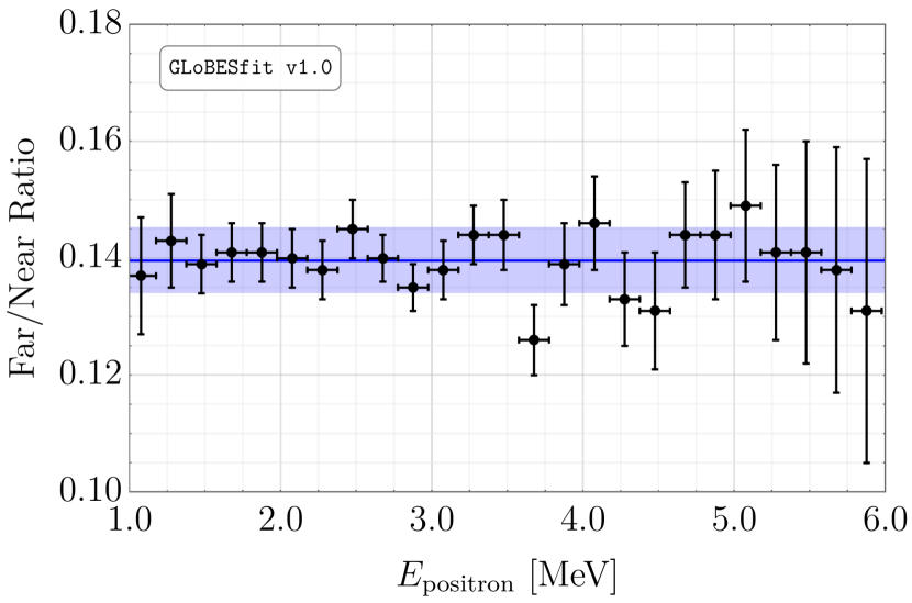
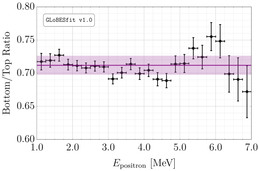
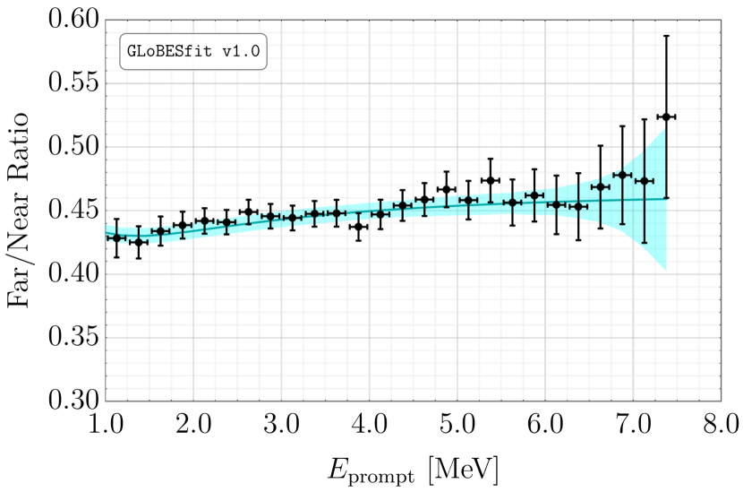
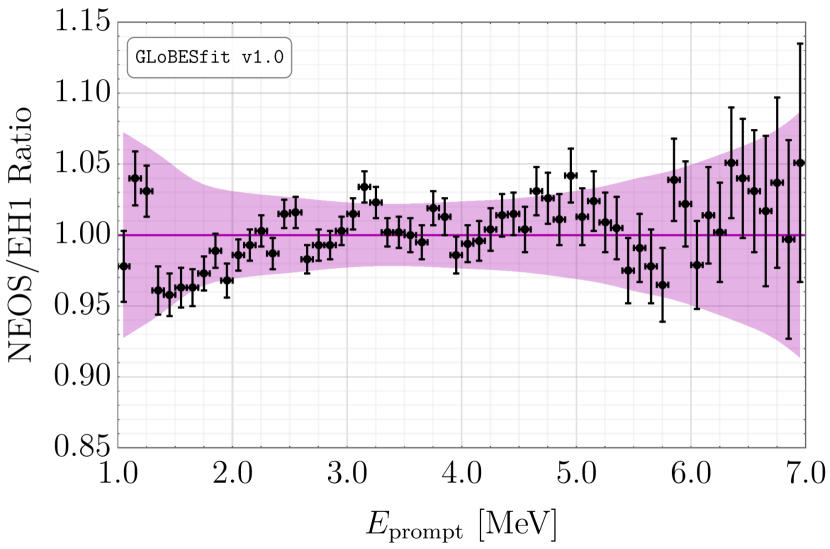
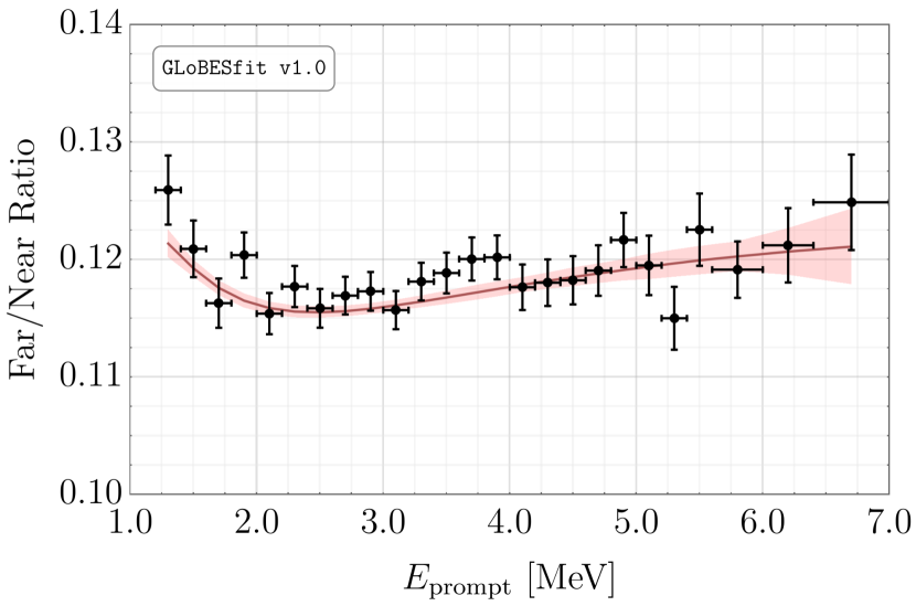
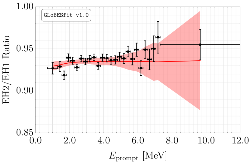
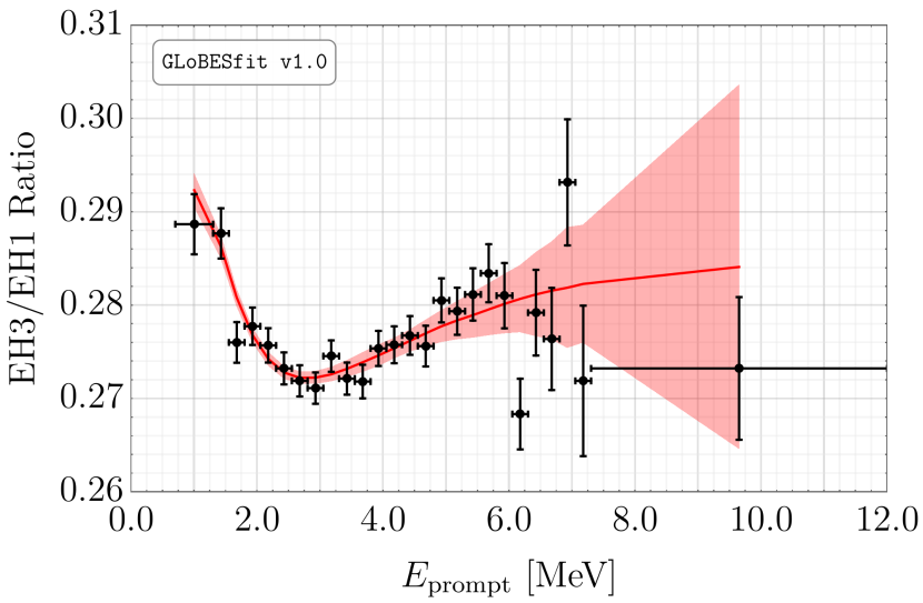
C.3 Markov Chain Monte Carlo Results
In Figs. 40 and 41, we show the result of our Markov-Chain Monte Carlo analyses described in Sec. VII. In the two-dimensional plots, the blue, orange and red contours represent the 68.3%, 95% and 99% credible regions (C.R.); the one-dimensional plots add to this list a green curve representing the 90% C.R. Above each one-dimensional figure is shown the best-fit value of the corresponding parameter, as well as extent of the 68.3% C.R. region. To determine the posterior probability, we use 100 chains of walkers with randomized starting points. Each walker takes 1500 steps, of which the first 500 are conservatively ignored for the purposes of burn-in. The calculations have been performed using emcee Foreman-Mackey et al. (2013).
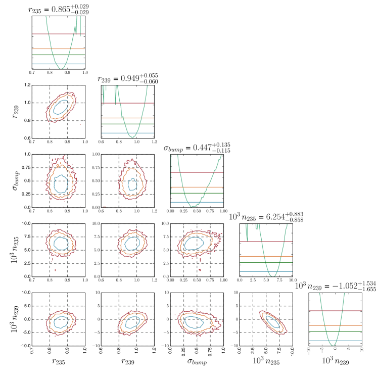
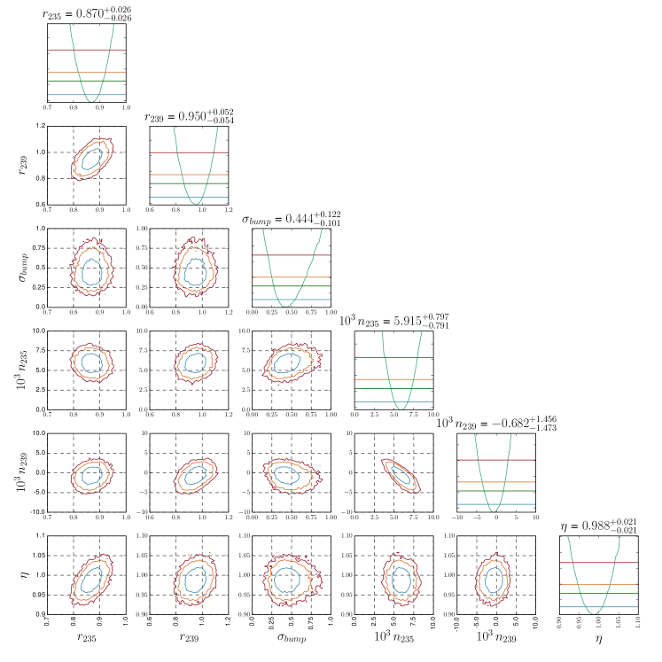
References
- Cowan et al. (1956) C. L. Cowan, F. Reines, F. B. Harrison, H. W. Kruse, and A. D. McGuire, “Detection of the free neutrino: A Confirmation,” Science 124, 103 (1956).
- Eguchi et al. (2003) K. Eguchi et al. (KamLAND), “First results from KamLAND: Evidence for reactor anti-neutrino disappearance,” Phys. Rev. Lett. 90, 021802 (2003), eprint hep-ex/0212021.
- An et al. (2012) F. P. An et al. (Daya Bay), “Observation of electron-antineutrino disappearance at Daya Bay,” Phys. Rev. Lett. 108, 171803 (2012), eprint 1203.1669.
- Ahn et al. (2012) J. K. Ahn et al. (RENO), “Observation of Reactor Electron Antineutrino Disappearance in the RENO Experiment,” Phys. Rev. Lett. 108, 191802 (2012), eprint 1204.0626.
- Abe et al. (2012) Y. Abe et al. (Double Chooz), “Indication of Reactor Disappearance in the Double Chooz Experiment,” Phys. Rev. Lett. 108, 131801 (2012), eprint 1112.6353.
- Carter et al. (1959a) R. E. Carter, F. Reines, J. J. Wagner, and M. E. Wyman, “Free anti-neutrino absorption cross-section. 2: Expected cross-section from measurements of fission fragment electron spectrum,” Phys. Rev. 113, 280 (1959a).
- Mention et al. (2011) G. Mention, M. Fechner, Th. Lasserre, Th. A. Mueller, D. Lhuillier, M. Cribier, and A. Letourneau, “The Reactor Antineutrino Anomaly,” Phys. Rev. D83, 073006 (2011), eprint 1101.2755.
- Mueller et al. (2011) Th. A. Mueller et al., “Improved Predictions of Reactor Antineutrino Spectra,” Phys. Rev. C83, 054615 (2011), eprint 1101.2663.
- Huber (2011) P. Huber, “On the determination of anti-neutrino spectra from nuclear reactors,” Phys. Rev. C84, 024617 (2011), [Erratum: Phys. Rev. C85, 029901 (2012)], eprint 1106.0687.
- Abazajian et al. (2012) K. N. Abazajian et al., “Light Sterile Neutrinos: A White Paper,” (2012), eprint 1204.5379.
- Hayes and Vogel (2016) A. C. Hayes and P. Vogel, “Reactor Neutrino Spectra,” Ann. Rev. Nucl. Part. Sci. 66, 219 (2016), eprint 1605.02047.
- Dentler et al. (2018) M. Dentler, A. Hernández-Cabezudo, J. Kopp, P. A. N. Machado, M. Maltoni, I. Martinez-Soler, and T. Schwetz, “Updated Global Analysis of Neutrino Oscillations in the Presence of eV-Scale Sterile Neutrinos,” JHEP 08, 010 (2018), eprint 1803.10661.
- Gariazzo et al. (2017) S. Gariazzo, C. Giunti, M. Laveder, and Y. F. Li, “Updated Global 3+1 Analysis of Short-BaseLine Neutrino Oscillations,” JHEP 06, 135 (2017), eprint 1703.00860.
- Aguilar-Arevalo et al. (2001) A. Aguilar-Arevalo et al. (LSND), “Evidence for neutrino oscillations from the observation of appearance in a beam,” Phys. Rev. D64, 112007 (2001), eprint hep-ex/0104049.
- Aguilar-Arevalo et al. (2013) A. A. Aguilar-Arevalo et al. (MiniBooNE), “Improved Search for Oscillations in the MiniBooNE Experiment,” Phys. Rev. Lett. 110, 161801 (2013), eprint 1303.2588.
- Diaz et al. (2019) A. Diaz, C. A. Argüelles, G. H. Collin, J. M. Conrad, and M. H. Shaevitz, “Where Are We With Light Sterile Neutrinos?,” (2019), eprint 1906.00045.
- Estienne et al. (2019) M. Estienne et al., “Updated Summation Model: An Improved Agreement with the Daya Bay Antineutrino Fluxes,” Phys. Rev. Lett. 123, 022502 (2019), eprint 1904.09358.
- Hayen et al. (2019) L. Hayen, J. Kostensalo, N. Severijns, and J. Suhonen, “First-forbidden transitions in the reactor anomaly,” (2019), eprint 1908.08302.
- Huber et al. (2005) P. Huber, M. Lindner, and W. Winter, “Simulation of long-baseline neutrino oscillation experiments with GLoBES (General Long Baseline Experiment Simulator),” Comput. Phys. Commun. 167, 195 (2005), eprint hep-ph/0407333.
- Huber et al. (2007) P. Huber, J. Kopp, M. Lindner, M. Rolinec, and W. Winter, “New features in the simulation of neutrino oscillation experiments with GLoBES 3.0: General Long Baseline Experiment Simulator,” Comput. Phys. Commun. 177, 432 (2007), eprint hep-ph/0701187.
- Berryman and Huber (2019) J. M. Berryman and P. Huber, “Reevaluating Reactor Antineutrino Anomalies with Updated Flux Predictions,” (2019), eprint 1909.09267.
- Choi et al. (2016) J. H. Choi et al. (RENO), “Observation of Energy and Baseline Dependent Reactor Antineutrino Disappearance in the RENO Experiment,” Phys. Rev. Lett. 116, 211801 (2016), eprint 1511.05849.
- An et al. (2016) F. P. An et al. (Daya Bay), “Measurement of the Reactor Antineutrino Flux and Spectrum at Daya Bay,” Phys. Rev. Lett. 116, 061801 (2016), [Erratum: Phys. Rev. Lett.118,no.9,099902(2017)], eprint 1508.04233.
- Abe et al. (2016) Y. Abe et al. (Double Chooz), “Measurement of θ13 in Double Chooz using neutron captures on hydrogen with novel background rejection techniques,” JHEP 01, 163 (2016), eprint 1510.08937.
- Carter et al. (1959b) R. E. Carter, F. Reines, J. J. Wagner, and M. E. Wyman, “Free antineutrino absorption cross section. ii. expected cross section from measurements of fission fragment electron spectrum,” Phys. Rev. 113, 280 (1959b), URL https://link.aps.org/doi/10.1103/PhysRev.113.280.
- Von Feilitzsch et al. (1982) F. Von Feilitzsch, A. A. Hahn, and K. Schreckenbach, “Experimental beta-spectra from 239Pu and 235U thermal neutron fission products and their correlated antineutrino spectra,” Phys. Lett. 118B, 162 (1982).
- Schreckenbach et al. (1985) K. Schreckenbach, G. Colvin, W. Gelletly, and F. Von Feilitzsch, “Determination of the antineutrino spectrum from 235U thermal neutron fission products up to 9.5 MeV,” Phys. Lett. 160B, 325 (1985).
- Hahn et al. (1989) A. A. Hahn, K. Schreckenbach, G. Colvin, B. Krusche, W. Gelletly, and F. Von Feilitzsch, “Antineutrino spectra from 241Pu and 239Pu thermal neutron fission products,” Phys. Lett. B218, 365 (1989).
- Adey et al. (2019a) D. Adey et al. (Daya Bay), “Measurement of Individual Antineutrino Spectra from and at Daya Bay,” (2019a), eprint 1904.07812.
- Ashenfelter et al. (2019) J. Ashenfelter et al. (PROSPECT), “Measurement of the Antineutrino Spectrum from 235U Fission at HFIR with PROSPECT,” Phys. Rev. Lett. 122, 251801 (2019), eprint 1812.10877.
- Vogel and Beacom (1999) P. Vogel and J. F. Beacom, “The angular distribution of the neutron inverse beta decay ,” Phys. Rev. D60, 053003 (1999), eprint hep-ph/9903554.
- (32) M. Fallot, Private Communication.
- Declais et al. (1994) Y. Declais et al., “Study of reactor anti-neutrino interaction with proton at Bugey nuclear power plant,” Phys. Lett. B338, 383 (1994).
- Giunti (2017) C. Giunti, “Precise determination of the 235U reactor antineutrino cross section per fission,” Phys. Lett. B764, 145 (2017), eprint 1608.04096.
- Kuvshinnikov et al. (1991) A. A. Kuvshinnikov, L. A. Mikaelyan, S. V. Nikolaev, M. D. Skorokhvatov, and A. V. Etenko, “Measuring the cross-section and beta decay axial constant in a new experiment at Rovno NPP reactor. (In Russian),” JETP Lett. 54, 253 (1991), [Sov. J. Nucl. Phys. 52, 300 (1990)].
- Declais et al. (1995) Y. Declais et al., “Search for neutrino oscillations at 15-meters, 40-meters, and 95-meters from a nuclear power reactor at Bugey,” Nucl. Phys. B434, 503 (1995).
- Zacek et al. (1986) G. Zacek et al. (CALTECH-SIN-TUM), “Neutrino Oscillation Experiments at the Gösgen Nuclear Power Reactor,” Phys. Rev. D34, 2621 (1986).
- Kwon et al. (1981) H. Kwon, F. Boehm, A. A. Hahn, H. E. Henrikson, J. L. Vuilleumier, J. F. Cavaignac, D. H. Koang, B. Vignon, F. Von Feilitzsch, and R. L. Mossbauer, “Search for Neutrino Oscillations at a Fission Reactor,” Phys. Rev. D24, 1097 (1981).
- Hoummada et al. (1995) A. Hoummada, S. Lazrak Mikou, M. Avenier, G. Bagieu, J. F. Cavaignac, and Dy. Holm Koan, “Neutrino oscillations I.L.L. experiment reanalysis,” Appl. Radiat. Isot. 46, 449 (1995).
- Vidyakin et al. (1987) G. S. Vidyakin, V. N. Vyrodov, I. I. Gurevich, Yu. V. Kozlov, V. P. Martemyanov, S. V. Sukhotin, V. G. Tarasenkov, and S. K. Khakimov, “Detection of Anti-neutrinos in the Flux From Two Reactors,” Sov. Phys. JETP 66, 243 (1987), [Zh. Eksp. Teor. Fiz. 93, 424 (1987)].
- Vidyakin et al. (1994) G. S. Vidyakin et al., “Limitations on the characteristics of neutrino oscillations,” JETP Lett. 59, 390 (1994), [Pisma Zh. Eksp. Teor. Fiz. 59, 364 (1994)].
- Kozlov et al. (2000) Yu. V. Kozlov, S. V. Khalturtsev, I. N. Machulin, A. V. Martemyanov, V. P. Martemyanov, S. V. Sukhotin, V. G. Tarasenkov, E. V. Turbin, and V. N. Vyrodov, “Antineutrino-Deuteron Experiment at the Krasnoyarsk Reactor,” Phys. Atom. Nucl. 63, 1016 (2000), [Yad. Fiz. 63, 1091 (2000)], eprint hep-ex/9912047.
- Greenwood et al. (1996) Z. D. Greenwood et al., “Results of a two position reactor neutrino oscillation experiment,” Phys. Rev. D53, 6054 (1996).
- Afonin et al. (1988) A. I. Afonin, S. N. Ketov, V. I. Kopeikin, L. A. Mikaelyan, M. D. Skorokhvatov, and S. V. Tolokonnikov, “A Study of the Reaction on a Nuclear Reactor,” Sov. Phys. JETP 67, 213 (1988), [Zh. Eksp. Teor. Fiz. 94 N2,1 (1988)].
- Kopeikin (2012) V. I. Kopeikin, “Flux and spectrum of reactor antineutrinos,” Phys. Atom. Nucl. 75, 143 (2012), [Yad. Fiz.75N2,165(2012)].
- Boireau et al. (2016) G. Boireau et al. (NUCIFER), “Online Monitoring of the Osiris Reactor with the Nucifer Neutrino Detector,” Phys. Rev. D93, 112006 (2016), eprint 1509.05610.
- Esteban et al. (2019) I. Esteban, M. C. Gonzalez-Garcia, A. Hernández-Cabezudo, M. Maltoni, and T. Schwetz, “Global analysis of three-flavour neutrino oscillations: synergies and tensions in the determination of , and the mass ordering,” JHEP 01, 106 (2019), eprint 1811.05487.
- Boehm et al. (2001) F. Boehm et al., “Final results from the Palo Verde neutrino oscillation experiment,” Phys. Rev. D64, 112001 (2001), eprint hep-ex/0107009.
- Miller (2001) L. H. Miller, Ph.D. thesis, Stanford U., Phys. Dept. (2001), URL http://wwwlib.umi.com/dissertations/fullcit?p3000068.
- (50) G. Gratta, Private Communication.
- Zhang et al. (2013) C. Zhang, X. Qian, and P. Vogel, “Reactor Antineutrino Anomaly with known ,” Phys. Rev. D87, 073018 (2013), eprint 1303.0900.
- Abe et al. (2014) Y. Abe et al. (Double Chooz), “Improved measurements of the neutrino mixing angle with the Double Chooz detector,” JHEP 10, 086 (2014), [Erratum: JHEP02,074(2015)], eprint 1406.7763.
- De Kerret et al. (2019) H. De Kerret et al. (Double Chooz), “First Double Chooz Measurement via Total Neutron Capture Detection,” (2019), eprint 1901.09445.
- Apollonio et al. (2003) M. Apollonio et al. (CHOOZ), “Search for neutrino oscillations on a long baseline at the CHOOZ nuclear power station,” Eur. Phys. J. C27, 331 (2003), eprint hep-ex/0301017.
- An et al. (2017a) F. P. An et al. (Daya Bay), “Improved Measurement of the Reactor Antineutrino Flux and Spectrum at Daya Bay,” Chin. Phys. C41, 013002 (2017a), eprint 1607.05378.
- An et al. (2017b) F. P. An et al. (Daya Bay), “Measurement of electron antineutrino oscillation based on 1230 days of operation of the Daya Bay experiment,” Phys. Rev. D95, 072006 (2017b), eprint 1610.04802.
- An et al. (2017c) F. P. An et al. (Daya Bay), “Evolution of the Reactor Antineutrino Flux and Spectrum at Daya Bay,” Phys. Rev. Lett. 118, 251801 (2017c), eprint 1704.01082.
- Adey et al. (2019b) D. Adey et al. (Daya Bay), “Improved Measurement of the Reactor Antineutrino Flux at Daya Bay,” Phys. Rev. D 100, 052004 (2019b), eprint 1808.10836.
- Giunti et al. (2019a) C. Giunti, Y. F. Li, B. R. Littlejohn, and P. T. Surukuchi, “Diagnosing the Reactor Antineutrino Anomaly with Global Antineutrino Flux Data,” Phys. Rev. D99, 073005 (2019a), eprint 1901.01807.
- (60) S.-B. Kim, Private Communication.
- Bak et al. (2019) G. Bak et al. (RENO), “Fuel-composition dependent reactor antineutrino yield at RENO,” Phys. Rev. Lett. 122, 232501 (2019), eprint 1806.00574.
- Bak et al. (2018) G. Bak et al. (RENO), “Measurement of Reactor Antineutrino Oscillation Amplitude and Frequency at RENO,” Phys. Rev. Lett. 121, 201801 (2018), eprint 1806.00248.
- Hayes et al. (2014) A. C. Hayes, J. L. Friar, G. T. Garvey, G. Jungman, and G. Jonkmans, “Systematic Uncertainties in the Analysis of the Reactor Neutrino Anomaly,” Phys. Rev. Lett. 112, 202501 (2014), eprint 1309.4146.
- Giunti et al. (2017) C. Giunti, X. P. Ji, M. Laveder, Y. F. Li, and B. R. Littlejohn, “Reactor Fuel Fraction Information on the Antineutrino Anomaly,” JHEP 10, 143 (2017), eprint 1708.01133.
- Gebre et al. (2018) Y. Gebre, B. Littlejohn, and P. Surukuchi, “Prospects for Improved Understanding of Isotopic Reactor Antineutrino Fluxes,” Phys. Rev. D 97, 013003 (2018), eprint 1709.10051.
- Gariazzo et al. (2018) S. Gariazzo, C. Giunti, M. Laveder, and Y. F. Li, “Model-independent short-baseline oscillations from reactor spectral ratios,” Phys. Lett. B782, 13 (2018), eprint 1801.06467.
- Alekseev et al. (2018) I. Alekseev et al. (DANSS), “Search for sterile neutrinos at the DANSS experiment,” Phys. Lett. B787, 56 (2018), eprint 1804.04046.
- Adey et al. (2018) D. Adey et al. (Daya Bay), “Measurement of the Electron Antineutrino Oscillation with 1958 Days of Operation at Daya Bay,” Phys. Rev. Lett. 121, 241805 (2018), eprint 1809.02261.
- Ko et al. (2017) Y.-J. Ko et al. (NEOS), “Sterile Neutrino Search at the NEOS Experiment,” Phys. Rev. Lett. 118, 121802 (2017), eprint 1610.05134.
- Almazán Molina et al. (2019) H. Almazán Molina et al. (STEREO), “Improved Sterile Neutrino Constraints from the STEREO Experiment with 179 Days of Reactor-On Data,” (2019), eprint 1912.06582.
- Ryder (2015) N. Ryder (SoLid), “First results of the deployment of a SoLid detector module at the SCK-CEN BR2 reactor,” PoS EPS-HEP2015, 071 (2015), eprint 1510.07835.
- Jacquemain et al. (2015) D. Jacquemain et al., Nuclear Power Reactor Core Melt Accidents: Current State of Knowledge (EDP Sciences, https://www.edp-open.org/images/stories/books/fulldl/Nuclear_Power_Reactor_Core_Melt_Accidents.pdf, 2015), ISBN 2759818358.
- (73) M. Danilov, “Search for sterile neutrinos at the DANSS experiment,”, URL http://www.solvayinstitutes.be/event/workshop/beyond_2018/slides/Danilov.pdf.
- Huber (2017) P. Huber, “NEOS Data and the Origin of the 5 MeV Bump in the Reactor Antineutrino Spectrum,” Phys. Rev. Lett. 118, 042502 (2017), eprint 1609.03910.
- Dentler et al. (2017) M. Dentler, A. Hernández-Cabezudo, J. Kopp, M. Maltoni, and T. Schwetz, “Sterile neutrinos or flux uncertainties? – Status of the reactor anti-neutrino anomaly,” JHEP 11, 099 (2017), eprint 1709.04294.
- Parke and Zukanovich-Funchal (2019) S. J. Parke and R. Zukanovich-Funchal, “Comment on Daya Bay’s Definition and Use of ,” (2019), eprint 1903.00148.
- Adey et al. (2019c) D. Adey et al. (Day Bay), “Comment on “Comment on Daya Bay’s Definition and Use of ” by S. Parke and R. Zukanovich Funchal,” (2019c), eprint 1905.03840.
- Maltoni and Schwetz (2003) M. Maltoni and T. Schwetz, “Testing the statistical compatibility of independent data sets,” Phys. Rev. D68, 033020 (2003), eprint hep-ph/0304176.
- Berryman et al. (2019) J. M. Berryman, V. Brdar, and P. Huber, “Particle physics origin of the 5 MeV bump in the reactor antineutrino spectrum?,” Phys. Rev. D99, 055045 (2019), eprint 1803.08506.
- Foreman-Mackey et al. (2013) D. Foreman-Mackey, D. W. Hogg, D. Lang, and J. Goodman, “emcee: The MCMC Hammer,” Publ. Astron. Soc. Pac. 125, 306 (2013), eprint 1202.3665.
- Serebrov et al. (2019) A. P. Serebrov et al. (NEUTRINO-4), “First Observation of the Oscillation Effect in the Neutrino-4 Experiment on the Search for the Sterile Neutrino,” Pisma Zh. Eksp. Teor. Fiz. 109, 209 (2019), [JETP Lett. 109, no. 4, 213 (2019)], eprint 1809.10561.
- (82) A. P. Serebrov, “Present status of Neutrino-4 experiment search for sterile neutrino,”, URL https://indico.cern.ch/event/833568/contributions/3655173/attachments/1957823/3252790/2-12_China_Serebrov_Neutrino-4.pdf.
- Giunti et al. (2019b) C. Giunti, Y. F. Li, and Y. Y. Zhang, “KATRIN bound on 3+1 active-sterile neutrino mixing and the reactor antineutrino anomaly,” (2019b), eprint 1912.12956.
- (84) J. M. Berryman, URL https://github.com/JMBerryman/GLoBESfit/releases.
- (85) J. M. Berryman and P. Huber, URL https://www.globesfit.org/.
- Feldman and Cousins (1998) G. J. Feldman and R. D. Cousins, “A Unified approach to the classical statistical analysis of small signals,” Phys. Rev. D57, 3873 (1998), eprint physics/9711021.
- Agostini and Neumair (2019) M. Agostini and B. Neumair, “Statistical Methods for the Search of Sterile Neutrinos,” (2019), eprint 1906.11854.
- Silaeva and Sinev (2020) S. V. Silaeva and V. V. Sinev, “Simulation of an experiment on looking for sterile neutrinos at nuclear reactor,” (2020), eprint 2001.10752.
- Giunti (2020) C. Giunti, “Statistical Significance of Reactor Antineutrino Active-Sterile Oscillations,” (2020), eprint 2004.07577.
- Ashenfelter et al. (2018) J. Ashenfelter et al. (PROSPECT), “First search for short-baseline neutrino oscillations at HFIR with PROSPECT,” Phys. Rev. Lett. 121, 251802 (2018), eprint 1806.02784.
- Danilov (2019) M. Danilov (DANSS), in 2019 European Physical Society Conference on High Energy Physics (2019), eprint 1911.10140.