Characterizing capacity of flexible loads for providing grid support

Abstract

Flexible loads are a resource for the Balancing Authority (BA) of the future to aid in the balance of supply and demand in the power grid. Consequently, it is of interest for a BA to know how much flexibility a collection of loads has, so to successfully incorporate flexible loads into grid level resource allocation. Loads’ flexibility is limited by all their Quality of Service (QoS) requirements. In this work we present a characterization of capacity for a collection of flexible loads. This characterization is in terms of the Power Spectral Density (PSD) of the reference signal. Two advantages of our characterization are: (i) it easily allows for a BA to use the characterization for resource allocation of flexible loads and (ii) it allows for precise definitions of the power and energy capacity for a collection of flexible loads.

I Introduction

The inherent variability in renewable generation sources such as solar and wind is a challenge for the power grid operators to balance demand and generation. Ramp rate constraints prevent conventional generation from handling this mismatch between demand and generation completely, while grid level storage from batteries is expensive. Thus a new resource is being investigated to help fill the mismatch: flexible loads. Flexible loads have the ability to vary power consumption over a baseline level without violating their Quality of Service (QoS). The baseline power consumption is the power consumed without grid interference. The requested amount from the grid authority, to deviate from baseline, is the reference signal. The tracking of a zero-mean reference signal guises, in the eyes of the grid operator, flexible loads as batteries providing storage services. This battery-like behavior of flexible loads is often referred as Virtual Energy Storage (VES) [1]. VES from flexible loads can be less expensive than energy storage from batteries [2]. Some examples of flexible loads include residential air conditioners [3], water heaters [4], refrigerators, commercial HVAC systems [5], pumps for irrigation [6], pool cleaning [7] or heating [8].

If the grid operator expects the flexible loads to track the reference signal accurately, then the reference must not cause the loads to violate their QoS. From the viewpoint of the grid operator, flexible loads not tracking a reference makes them appear unreliable. From the viewpoint of the load, reference signals that continually require QoS violation provide incentive for loads to stop providing VES. In either case, avoidance of the above scenarios is paramount to the long term success of VES. That is, reference signals must be designed to respect the capacity of the collection of flexible loads.

Informally, the capacity represents limitations in ensemble behavior (e.g., the ability to track a reference signal) due to QoS requirements at the individual load. Consequently, a key step in determining the capacity is relating the QoS requirements to requirements for the reference signal. Unfortunately, this is not a straight forward task and many varying approaches are present in the current literature [9, 10, 11, 12, 13, 14]. The most popular approach is to develop ensemble level necessary conditions [11, 9]; reference signals that satisfy these conditions ensure the ability of all loads in the collection to satisfy QoS while tracking the reference. Other approaches include geometry based characterizations [15] and characterizations through distributed optimization [16].

A limitation of the currently available capacity results is that a balancing authority requires a specific reference signal to perform resource allocation; only post-facto checking if the BA’s needs are within the capacity of the resource is possible. That is, these capacity characterizations cannot be used for long-term planning. The BA’s need are exogenous, so a useful capacity characterization should allow the BA to determine the portion of its needs that can be provided by a specific class and number of loads ahead of time.

Contrarily, if one develops constraints on the statistics of the reference signal, then a notion of capacity that is also useful for planning can be developed. For instance, consider Figure 1 where the Power Spectral Density (PSD) of a grid’s net demand is allocated to resources (precise definition of PSDs is provided later). This frequency based allocation does not require knowledge of a specific reference signal, but only of the statistics of the reference signal. To avoid possible confusion with electrical power (in Watt) we use Spectral Density (SD) instead of Power Spectral Density (PSD) in the rest of the paper.

In fact, it was introduced in [17] that the QoS requirements of flexible loads can be characterized as constraints in the frequency domain. That is, while primarily an illustrative example, it is possible to quantitatively develop the regions shown in Figure 1.

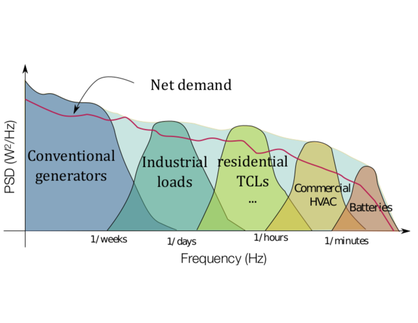
Figure 1: An example spectral allocation of resources to meet the grids needs.

In addition to [17, 18], there are many works that advocate for the specification of loads’ abilities [19, 5] and for resource allocation spectrally [20]. The results of real world VES experiments also suggest that specifying the spectral content of a reference signal is a feasible way to encapsulate the limitations in flexibility of a load [21]. A simplification of this concept is also widely used in today’s power grid; ancillary services are classified by their response times and ramp rates [22].

Motivated by the advantages of working in the frequency domain we extend the work in [17, 18] and characterize the capacity through the SD of the reference signal, for an entire collection of flexible loads, based on the QoS requirements of each flexible load. The QoS constraints considered here are quite general and encapsulate operating constraints for: (i) Commercial HVAC systems, (ii) batteries, and (iii) Thermostatically Controlled Loads (TCLs). The contribution over past work is threefold: (i) we characterize capacity through constraints on the statistics of the reference signal, rather than the reference signal itself, (ii) our characterization of capacity allows for a BA to easily perform resource allocation and (iii) our characterization allows for precise definitions of the power and energy capacity for a collection of flexible loads.

We corroborate the advantages of our capacity characterization through numerical experiments. A convex optimization problem is setup that ‘projects’ the needs of the grid authority onto the set of feasible SD’s. The needs of the grid is quantified as the SD of net-demand, as seen in Figure 1. In each simulation scenario, we determine the power and energy capacity of a collection of flexible loads based on the obtained SD.

The capacity characterization presented is for continuously varying loads, that is loads that can vary power consumption freely within an interval. The capacity characterization can be extended to handle discrete loads (e.g., TCLs), by applying it to the work [11].

A preliminary version of this work is published in [18], which dealt with a single load. In this work we extend the results to a collection of loads.

The paper proceeds as follows, Section II describes the QoS constraints of loads, Section III describes mathematical prerequisites and a characterization of individual load capacity, Section IV describe the spectral characterization of the constraints for the ensemble. Section V describes the method for determining how much of a grid’s needs can be satisfied by flexible loads. Numerical results are provided in Section VI.

II QoS Constraints of Individuals

Denote by $P(t)$ the power consumption of a VES system at time $t$, and let $P^{b}(t)$ its baseline demand. The demand deviation is $\tilde{P}:=P(t)-P^{b}(t)$, and for the load to provide VES service by controlling the deviation $\tilde{P}(t)$ to track some reference signal. The first constraint is simply an actuator constraint:

$$\text{QoS-1:}\quad\left|\tilde{P}(t)\right|\leq c_{1},\quad\forall\ t,$$ (1)

where the constant $c_{1}$, the maximum possible deviation of power consumption, depends on the rated power and the baseline demand. Second, define the demand increment $\tilde{P}_{\delta}(t):=\tilde{P}(t)-\tilde{P}(t-\delta)$, where $\delta>0$ is a predetermined (small) time interval. The second constraint is a ramping rate constraint:

$$\text{QoS-2:}\quad\left|\tilde{P_{\delta}}(t)\right|\leq c_{2},\quad \forall\ t.$$ (2)

Third, define the additional energy use during any time interval of length $T$:

$$\tilde{E}(t)=\int_{t-T}^{t}\tilde{P}(\sigma)d\sigma.$$ (3)

Since (3) is a linear system it has representation with Laplace variable: $\tilde{E}(s)=G(s)\tilde{P}(s)$ for some BIBO stable transfer function $G$. The third QoS constraint is that

$$\text{QoS-3:}\quad\left|\tilde{E}(t)\right|\leq c_{3},\quad \forall\ t.$$ (4)

The parameter $T$ in (3) can represent the length of a billing period. Ensuring (4) ensures that the energy consumed during a billing period close to the nominal energy consumed, although it is stronger than what is necessary.

To define the fourth and last QoS constraint, we associate with the VES system a storage variable $\theta$ that is related to the demand deviation through a stable linear time invariant system $H(s)$ as follows:

$$\tilde{\theta}(s)=H(s)\tilde{P}(s),$$ (5)

and impose the constraint

$$\text{QoS-4:}\quad\left|\tilde{\theta}(t)\right|\leq c_{4},\quad \forall\ t.$$ (6)

To understand the storage variable, imagine the VES system is a flexible HVAC system. A simple model of the indoor temperature of a building this HVAC system serves is:

$$C\dot{\theta}(t)=\frac{1}{R}\left(\theta_{0}(t)-\theta(t)\right)+\dot{q}_{\text{\scriptsize int}}(t)+\eta_{\text{\tiny COP}}P(t),$$ (7)

where $C$ and $R$ are thermal capacitance and resistance, $\theta_{0}(t)$ is the ambient temperature, $\eta_{\text{\tiny COP}}$ is the coefficient of performance, and $\dot{q}_{\text{\scriptsize int}}(t)$ is an internal disturbance.

In general, the baseline power consumption for a HVAC system is the value $P^{b}(t)$ that keeps the internal temperature of the load at a fixed value $\bar{\theta}$, which for (7) is

$$P^{b}(t)=-\frac{\left(\theta_{0}(t)-\bar{\theta}\right)}{\eta_{\text{\tiny COP}}R}-\frac{\dot{q}_{\text{\scriptsize int}}(t)}{\eta_{\text{\tiny COP}}}.$$ (8)

Since we are concerned with the flexibility in the load, we linearize (7) about the thermal setpoint $\bar{\theta}$ and the baseline power $P^{b}(t)$ yielding,

$$\dot{\tilde{\theta}}(t)=-\gamma\tilde{\theta}(t)+\beta\tilde{P}(t),\quad\gamma=\frac{1}{RC},\quad\beta=\frac{\eta_{\text{\tiny COP}}}{C},$$ (9)

where $\tilde{\theta}\triangleq\theta(t)-\bar{\theta}$ is the internal temperature deviation and $\tilde{P}$ is as defined at the beginning of this Section.

Taking the Laplace transform of (9), we get $\tilde{\theta}(s)=\frac{\beta}{s+\gamma}\tilde{P}(s)$. So, for the HVAC system example, the storage variable is simply the indoor temperature deviation from the baseline value, and $H(s)=\frac{\beta}{s+\gamma}$. A more complex model of HVAC dynamics would lead to a higher order $H(s)$. The model (7), while simplistic, has been shown to agree quite well with more realistic models for certain flexible loads [23].

Also, when the VES system is in fact a battery, $\tilde{\theta}(t)$ can be thought of a the amout of energy stored in the battery at time $t$, i.e., $\tilde{\theta}=E_{0}x_{\text{\scriptsize SoC}}(t)$, where $E_{0}$ is the nominal energy capacity in kWh and $x_{\text{\scriptsize SoC}}$ is the state of charge. A simple dynamic model of this variable is $\dot{\tilde{\theta}}(t)=-\alpha\tilde{\theta}(t)+\tilde{P}(t)$, where $-\alpha\tilde{\theta}(t)$ accounts for the leakage, self degradation, and non-unity round trip efficiency of the battery. In this case $H(s)=\frac{1}{s+\alpha}$

The four constraints QoS 1-4, with parameters $Q^{i}\triangleq\left(\{c_{i}\}_{i=1}^{4},T,\delta\right)^{i}$ specify the QoS set for the VES system. The concern now is, what is a feasible power deviation signal $\tilde{P}(t)$?

III Individual Load Capacity

III-A Stochastic Setting

To develop our capacity characterization, we switch from a deterministic to a stochastic setting. In this setting we model the power deviation, $\tilde{P}$ as a continuous time stochastic process. The mean and autocorrelation function for $\tilde{P}$ are,

$$\mu_{\tilde{P}}(t) \triangleq\mathbf{E}[\tilde{P}(t)],\quad\forall\ t,$$ (10)

$$R_{\tilde{P}}(s,t) \triangleq\mathbf{E}[\tilde{P}(s)\tilde{P}(t)],\ \forall\ s,t,$$ (11)

where $\mathbf{E}[\cdot]$ denotes mathematical expectation. We make the following assumption about the stochastic process $\tilde{P}$.

Assumption 1.

The stochastic process $\tilde{P}$ is wide sense stationary (WSS) with mean function $\mu_{\tilde{P}}=0$ for all $t$.

Since $\tilde{P}$ is expressed as the difference of the power consumption from a base value it is intuitive to set the expectation of this to zero. Otherwise, loads are not providing storage services. Furthermore, WSS requires the variance and mean of the process $\tilde{P}$ to be time invariant and the autocorrelation function to be a function of $\tau=s-t$. We denote the time invariant variance as $\sigma^{2}_{\tilde{P}}$; the time invariant mean is already specified in the assumption.

In addition, for a continuous time WSS stochastic process $\{X(t)\}$ we have, through the Fourier transform, an alternative expression for the autocorrelation function [24],

$$R_{X}(\tau)=\int_{-\infty}^{\infty}S_{X}(\omega)e^{(j\omega\tau)}d\frac{\omega}{2\pi},\ \text{and}$$ (12)

$$S_{X}(\omega)=\int_{-\infty}^{\infty}R_{X}(\tau)e^{(-j\omega\tau)}d\tau,$$ (13)

where $S_{X}(\omega)$ is the (power) Spectral Density (SD) of $X$, $\omega\in\mathbb{R}$ is the frequency variable, and $j$ is the imaginary unit. The above is based on the general definition for (power) SD of the signal $X$,

$$S_{X}(\omega)\triangleq\lim_{T\to\infty}\frac{1}{T}\mathbf{E}\bigg{[}\bigg{|}\int_{0}^{T}X(t)e^{-j\omega t}\bigg{|}^{2}\bigg{]}$$ (14)

the equivalence of definitions (14) and (13) for a WSS process is the Wiener-Khinchin theorem. Letting $\tau=0$ in (12) results in,

$$R_{X}(0)=\int_{-\infty}^{\infty}S_{X}(\omega)d\frac{\omega}{2\pi},$$ (15)

where, if the mean of $X$ is zero, $R_{X}(0)$ is the variance of the process $X$. We introduce the following proposition from [24] that will be useful in the developments to follow.

Proposition 1.

[24] Let X be a WSS stochastic process and input to the linear time invariant BIBO stable system $G(s)$ with output $Y$, then $Y$ is WSS, $X$ and $Y$ are jointly WSS, and

(i) $$\mathbf{E}[Y]=G\left(j\omega\right)\Big{|}_{\omega=0}\mathbf{E}[X],$$

(ii) $$S_{Y}(\omega)=\left|G(j\omega)\right|^{2}S_{X}(\omega),$$

where $S_{X}$ is the SD of $X$, $S_{Y}$ is the SD of $Y$, and $G(j\omega)$ is the frequency response of $G(s)$.

Furthermore, the Chebyshev inequality for a random variable $X$, will be useful:

$$\mathcal{P}\big{(}\left|X-\mu_{\tiny X}\right|\geq k\big{)}\leq\frac{\sigma^{2}_{X}}{k^{2}},\quad\forall\ k>0,$$ (16)

where $\mathcal{P}(\cdot)$ denotes probability.

III-B Inequality Constraints: Spectral Characterization

The QoS constraints QoS 1-4 are characterized probabilistically in the following way. The inequalities in QoS 1-4 turn into probabilistic inequalities; the probability of the QoS constraint not being met is required to be small:

$$\mathcal{P}\left(\left|{\tilde{P}(t)}\right|\geq c_{1}\right)\leq\epsilon_{1}, \forall\ t,$$ (17)

$$\mathcal{P}\left(\left|\tilde{P}_{\delta}(t)\right|\geq c_{2}\right)\leq\epsilon_{2}, \forall\ t,$$ (18)

$$\mathcal{P}\left(\left|\tilde{E}(t)\right|\geq c_{3}\right)\leq\epsilon_{3}, \forall\ t,$$ (19)

$$\mathcal{P}\left(\left|\tilde{\theta}(t)\right|\geq c_{4}\right)\leq\epsilon_{4}, \forall\ t,$$ (20)

The quantities $\{\epsilon_{i}\}_{i=1}^{4}$ set the tolerance level for satisfying the respective constraint and are chosen to be small.

In order to pose the inequality constraints (17)-(20) in terms of $S_{\tilde{P}}$, two steps are taken. The first step is to utilize the Chebyshev inequality (16) to bound the probabilities in (17)-(20) as a function of the variance of the given random variable. The second step is to then use the Wiener-Khinchin theorem (12) to express the variance as the integral of $S_{\tilde{P}}$.

Lemma 1.

Let $\tilde{P}$ satisfy Assumption 1, then for all $t$,

$$\mathbf{E}[\tilde{E}(t)]=0,\ \mathbf{E}[\tilde{P}_{\delta}(t)]=0,\ \text{and}\ \mathbf{E}[\tilde{\theta}(t)]=0.$$

Proof.

Apply the result of Proposition 1-(i) for $\mathbf{E}[\tilde{E}(t)]$ and $\mathbf{E}[\tilde{\theta}(t)]$. The linearity of expectation suffices for $\mathbf{E}[\tilde{P}_{\delta}(t)]$. ∎

With the result in Lemma 1 and Chebyshev’s inequality (16) we formulate sufficient conditions for the inequality constraints (17)-(19) as follows,

$$\sigma_{\tilde{P}}^{2}\leq{c_{1}^{2}}\epsilon_{1}, \sigma^{2}_{\tilde{P}_{\delta}}\leq{c_{2}^{2}}\epsilon_{2},$$ (21)

$$\sigma^{2}_{\tilde{E}}\leq{c_{3}^{2}}\epsilon_{3} \sigma^{4}_{\tilde{\theta}}\leq{c_{4}^{2}}\epsilon_{4},$$ (22)

so that the probability of exceeding the inequality constraints (17)-(20) will be less than the respective specified amount, $\{\epsilon_{i}\}_{i=1}^{4}$. The variance $\sigma^{2}_{\tilde{P}_{\delta}}$ is equivalently,

$$\sigma^{2}_{\tilde{P}_{\delta}}=\mathbf{E}\bigg{[}\left(\tilde{P}_{\delta}(t)\right)^{2}\bigg{]}=2\left(R_{\tilde{P}}(0)-R_{\tilde{P}}(\delta)\right),$$ (23)

Now applying the Wiener-Khinchin theorem (12) to the LHS of (21)-(22) we have,

$$\int_{0}^{\infty}S_{\tilde{P}}(\omega)d\frac{\omega}{\pi}\leq{c_{1}^{2}}\epsilon_{1},$$ (24)

$$\int_{0}^{\infty}S_{\tilde{P}}(\omega)\left(2-2\cos{(\omega\delta)}\right)d\frac{\omega}{\pi}\leq\epsilon_{2}c_{2}^{2},$$ (25)

$$\int_{0}^{\infty}S_{\tilde{E}}(\omega)d\omega=\int_{0}^{\infty}|G(j\omega)|^{2}S_{\tilde{P}}(\omega)d\frac{\omega}{\pi}\leq{c_{4}^{2}}\epsilon_{4},$$ (26)

$$\int_{0}^{\infty}S_{\tilde{\theta}}(\omega)d\frac{\omega}{\pi}=\int_{0}^{\infty}|H(j\omega)|^{2}S_{\tilde{P}}(\omega)d\frac{\omega}{\pi}\leq{c_{3}^{2}}\epsilon_{3}.$$ (27)

Definition 1.

(Individual load constraint set) The set of feasible SDs is,

$$\mathcal{S}=\{S_{\tilde{P}}\ :\ S_{\tilde{P}}\geq 0,\ \text{and}\ \eqref{eq:intPowerDev}-\eqref{eq:intEngDev}\}.$$

That is, if $\tilde{P}$ has SD in the set $\mathcal{S}$, then the loads power deviation can match $\tilde{P}$ while satisfying the constraints (17)-(20).

III-C Power and energy capacity

Utilizing the concept of SD, the definition of power and energy capacity of a flexible load can be characterized in terms of the SD of the power deviation.

Definition 2.

Let $\epsilon\in(0,1]$ and $\mathcal{S}_{\epsilon}$ be a set of SDs, then the power and energy capacity for a given SD $S\in\mathcal{S}_{\epsilon}$ are,

$$\textbf{Pow}(S) =\sqrt{\frac{1}{\pi\epsilon}\int_{0}^{\infty}S(\omega)d\omega}\quad(W),$$

$$\textbf{Eng}(S) =\sqrt{\frac{1}{\pi\epsilon}\int_{0}^{\infty}\left|G(j\omega)\right|^{2}S(\omega)d\omega}\quad(Wh),$$

The reason for these definitions is that for a signal $\tilde{P}(t)$ with SD $S$, the following inequalities follow from these definitions upon applying (3):

$$\mathcal{P}\left(\left|\tilde{P}(t)\right|\geq\textbf{Pow}(S)\right)\leq\epsilon,\forall t$$ (28)

$$\mathcal{P}\left(\left|\tilde{E}(t)\right|\geq\textbf{Eng}(S)\right)\leq\epsilon,\forall t.$$ (29)

The set $\mathcal{S}_{\epsilon}$ is given explicit dependence on $\epsilon$ to reflect the dependence of constraints (24)-(26) on $\epsilon$.

For clarity, we estimate these probabilities for a given $\epsilon$ and SD $S\in\mathcal{S}_{\epsilon}$. We denote the estimated probabilities as $\hat{P}_{i}(\cdot)$ which are estimated by obtaining a time series of length $N$ with the desired SD and computing,

$$\hat{\mathcal{P}}_{i}\left(\left|\tilde{P}\right|\geq\textbf{Pow}(S)\right)=\frac{1}{N}\sum_{k=1}^{N}\mathbf{1}\left(\left|\tilde{P}_{k}\right|\geq\textbf{Pow}(S)\right)$$

The results are repeated for $2\times 10^{4}$ trials, and are shown in Figures 3-3 as a histogram, with values typically well below the respective thresholds. In addition, we plot two generated time series sample paths in Figures 5-5. The two sample paths are typically within the power and energy capacity bounds defined.

Thus for a SD $S$, the power and energy capacity defined in Definition 2 encompass maximum probabilistic limits, i.e., the capacity, for a time series that is associated with the SD $S$.

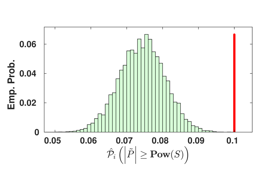
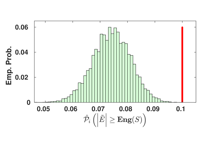
Figure 2: Empirically estimated probability bounds for the power capacity with $\epsilon_{1}=0.1$.

Figure 3: Empirically estimated probability bounds for the energy capacity with $\epsilon_{4}=0.1$.

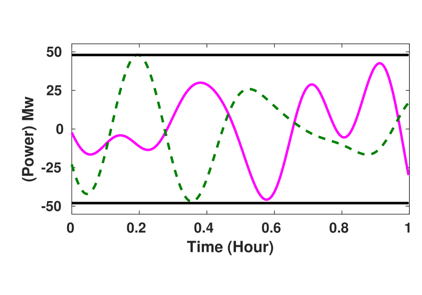
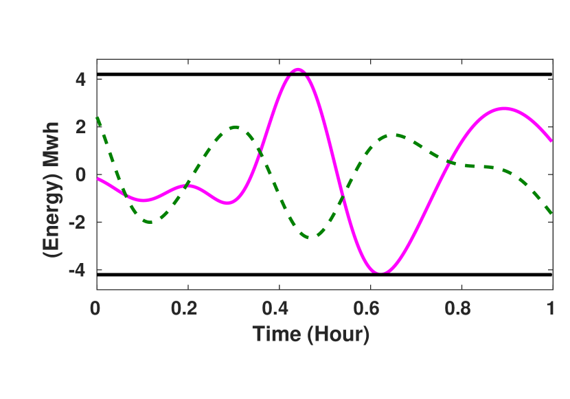
Figure 4: Two sample paths of a power consumption trajectory.

Figure 5: Two sample paths of an energy consumption trajectory.

Definition 3.

Let $\epsilon\in(0,1]$ and $S\in\mathcal{S}_{\epsilon}$ with power and energy capacity $\textbf{Pow}(S)$ and $\textbf{Eng}(S)$, respectively, then the un-used power and energy capacity is

$$\mathcal{U}_{\textbf{Pow}}(S) =c_{1}\left(1-\frac{\textbf{Pow}(S)}{c_{1}}\right)\quad(W),$$ (30)

$$\mathcal{U}_{\textbf{Eng}}(S) =c_{4}\left(1-\frac{\textbf{Eng}(S)}{c_{4}}\right)\quad(Wh),$$ (31)

where $c_{1}$ and $c_{4}$ are as used in (1) and (4), respectively.

IV Ensemble Capacity

Section III constructed constraints on the SD $S_{\tilde{P}}$ so to respect the capacity requirements for an individual load. In this section we do the same for $n$ loads. This is achieved by defining an “ensemble SD” and utilizing the constraints on the individuals to develop constraints for the ensemble SD. First, the ensemble power deviation is defined as

$$\bar{P}(t)\triangleq\sum_{i=1}^{n}\tilde{P}^{i}(t).$$ (32)

The ensemble SD is then the SD of $\bar{P}(t)$, that is,

$$S_{\bar{P}}(\omega)=\int_{-\infty}^{\infty}R_{\bar{P}}(\tau)e^{-j\omega\tau}d\tau,$$ (33)

where $R_{\bar{P}}(\tau)$ is the autocorreleation function of $\bar{P}$. With the requirement that each $\tilde{P}^{i}(t)$ is jointly WSS, the ensemble power deviation (32) is also WSS and the definition (33) is valid.

Figure 6: An example control architecture for flexible loads to assist the grid.

The SD of the sum, being the Fourier transform of the autocorrelation of the sum, depends on how the component signals $\tilde{P}^{i}$ are correlated to one another. In the limiting case when they are uncorrelated with one another, the autocorrelation of the sum is the sum of the autocorrelations since the cross correlations are 0. In that case the SD of the sum is also the sum of the SDs. Similarly, in the limiting cases of being perfectly anti-correlated or correlated, one can come up with precise relationship. However, the most interesting case from a practical point of view is when they signals are positively correlated but without having a perfect correlation of 1. To understand the reason, let us imagine how these signals $\tilde{P}^{i}$ will be generated. It is reasonable to assume a control architecture shows in Figure 6: a regulation signal from the balancing authority, $r(t)$, is split into $n$ distinct components, $r_{i}(t)$, $i=1,\dots,n$, so that $r_{i}(t)$ is within the capacity of load $i$, and some control system is used to ensure that $\tilde{P}^{i}$ tracks $r_{i}$. For instance, $r_{i}$ can be computed by band-pass filtering $r$ with a filter $F_{i}(j\omega)$. In a well designed system, these filters will ensure that the signals $r_{i}$ have sufficient positive correlation. Otherwise, each load - assuming they perfectly track their references - will be working against each other instead of working collaboratively to supply the total $r$. Although the design of the coordination architecture for the loads is beyond the scope of this work, we make the following assumption:

Assumption 2.

For any pair of loads $\ell,m$, $E[\tilde{P}_{\ell}(t)\tilde{P}_{m}(t+\tau)]=:R_{\ell,m}(\tau)\geq 0$ for every $\tau$.

Lemma 2.

The ensemble SD of $n$ loads, under Assumption 2, satisfies

$$\Sigma_{\bar{P}}\leq S_{\bar{P}}\leq n\Sigma_{\bar{P}},$$ (34)

where $\Sigma_{\bar{P}}:=\sum_{i=1}^{n}S_{\tilde{P}^{i}}$.

Proof.

Since the signals in the sum are jointly WSS, we have

$$R_{\bar{P}(t),\bar{P}(t)}(\tau)=\sum_{\ell=1}^{n}\sum_{m=1}^{n}R_{\ell,m}(\tau).$$ (35)

The cross correlation $R_{\ell,m}(\tau)$ when $\ell\neq m$ is non negative by Assumption 2 (the first one), $R_{\bar{P}(t),\bar{P}(t)}(\tau)\geq\sum_{\ell=1}^{n}R_{\ell,\ell}(\tau)$, from which the lower bound follows due to linearity of the Fourier transform. The upper bound is proven by considering the definition (14) for $S_{\bar{P}}(\omega)$. We have for all $\omega\in\mathbb{R}$, $S_{\bar{P}}(\omega)=$

$$\lim_{T\to\infty}\frac{1}{T}\mathbf{E}\bigg{[}\bigg{|}\sum_{i=1}^{n}\int_{0}^{T}\tilde{P}^{i}(t)e^{-j\omega t}\bigg{|}^{2}\bigg{]}$$ (36)

$$\leq\lim_{T\to\infty}\frac{n}{T}\sum_{i=1}^{n}\mathbf{E}\bigg{[}\bigg{|}\int_{0}^{T}\tilde{P}^{i}(t)e^{-j\omega t}\bigg{|}^{2}\bigg{]}=n\Sigma_{\bar{P}}(\omega),$$ (37)

where the bound is from Jensen’s inequality: $\left|\sum_{i=1}^{n}x_{i}\right|^{2}\leq n\sum_{i=1}^{n}\left|x_{i}\right|^{2}$ since $\left|\cdot\right|^{2}$ is convex. ∎

Corollary 1.

For a homogeneous collection of $n$ loads in which $P_{\ell}(t)=P_{m}(t)$ for every $\ell,m=1,\dots,n$, the ensemble SD is

$$S_{\bar{P}}=n\Sigma_{\bar{P}}.$$

The proof follows from the same argument used in establishing the upper bound case of Lemma 2.

In addition, for a heterogeneous ensemble the lower bound in Lemma 2 will be loose as $n$ increases. A better bound can be obtained by ‘binning’ the heterogeneous collection into several homogeneous ensembles and utilizing the result of Corollary 1.

Corollary 2.

For a heterogeneous collection of $n$ loads with $n_{\text{bin}}$ bins indexed by $\ell$ with $n_{\ell}$ loads in the $\ell^{th}$ bin, the ensemble SD is bounded as,

$$\sum_{\ell=1}^{n_{\text{bin}}}n_{\ell}\Sigma_{\bar{P}^{\ell}}\leq S_{\bar{P}}\leq n_{\text{bin}}\sum_{\ell=1}^{n_{\text{bin}}}n_{\ell}\Sigma_{\bar{P}^{\ell}},$$

with

$$\Sigma_{\bar{P}^{\ell}}\triangleq\sum_{(i\ \in\ \text{bin}\ \ell)}S_{\tilde{P}^{i}}.$$

Proof.

Apply directly the same procedure as in Lemma 2, except for $n_{\text{bin}}$ loads with the $\ell^{th}$ SD being $n$$\Sigma_{\bar{P}^{\ell}}$ (Corollary 1). ∎

IV-A Ensemble constraint set

We now develop a constraint set on $\Sigma_{\bar{P}^{\ell}}$  based on the set of constraints for the individual SDs that are in the definition of $\Sigma_{\bar{P}^{\ell}}$. In light of the results of Corollary 2, we assume a homogeneous collection of loads. The idea is to sum the individual constraints over $n_{\ell}$ so that the definition of $\Sigma_{\bar{P}^{\ell}}$ can be inserted. We do this for the rate constraint below,

$$\sum_{(i\ \in\ \text{bin}\ \ell)}\int_{0}^{\infty}\left(1-\cos(\omega\delta)\right)S_{\tilde{P}^{i}}(\omega)d\omega\leq n_{\ell}\frac{\pi\epsilon_{2}c^{2}_{2}}{2},$$

$$\iff\int_{0}^{\infty}\left(1-\cos(\omega\delta)\right)\Sigma_{\bar{P}^{\ell}}(\omega)d\omega\leq n_{\ell}\frac{\pi\epsilon_{2}c^{2}_{2}}{2}.$$

The other constraints are obtained in a similar fashion, and the full constraint set for $\Sigma_{\bar{P}^{\ell}}$ is: $\mathcal{S}(n_{\text{bin}},n_{\ell},\ell)\triangleq$

$$\bigg{\{} \Sigma_{\bar{P}^{\ell}}\ :\ \Sigma_{\bar{P}^{\ell}}\geq 0,$$

$$\int_{0}^{\infty}\Sigma_{\bar{P}^{\ell}}(\omega)d\omega\leq n_{\text{bin}}n_{\ell}\bigg{(}\pi\epsilon_{1}c_{1}^{2}\bigg{)},$$

$$\int_{0}^{\infty}(1-\cos{(\omega\delta)})\Sigma_{\bar{P}^{\ell}}(\omega)d\omega\leq n_{\text{bin}}n_{\ell}\bigg{(}\frac{\pi\epsilon_{2}c_{2}^{2}}{2}\bigg{)},$$

$$\int_{0}^{\infty}\left|G(j\omega)\right|^{2}\Sigma_{\bar{P}^{\ell}}(\omega)d\omega\leq n_{\text{bin}}n_{\ell}\bigg{(}\pi\epsilon_{3}c_{3}^{2}\bigg{)},$$

$$\int_{0}^{\infty}\left|H(j\omega)\right|^{2}\Sigma_{\bar{P}^{\ell}}(\omega)d\omega\leq n_{\text{bin}}n_{\ell}\bigg{(}\pi\epsilon_{4}c_{4}^{2}\bigg{)}\bigg{\}}.$$

The sets $\mathcal{S}(1,n_{\ell},\ell)$ and $\mathcal{S}(n_{\text{bin}},n_{\ell},\ell)$ represent the constraint set for the $\ell^{th}$ SD in the lower and upper bounds in Corollary 2, respectively. Additionally, $\mathcal{S}(1,n,1)$ exactly represents the constraint set for the single ensemble SD in Corollary 1 of a homogeneous ensemble with $n$ loads.

V Resource Allocation for Flexible Loads

We illustrate here how the ensemble constraint set in Section IV can be used by a Balancing Authority (BA) for resource allocation. Conceptually, our proposed method “projects” the needs of the BA onto the ensemble constraint set. We first describe how a BA can incorporate the ensemble constraint set into an optimization problem for resource allocation and then how a BA can determine its needs spectrally.

V-A Allocation through projection

We denote by $S^{\text{\scriptsize BA}}(\omega)$ a SD that represents the BA’s needs. Computation of this SD will be discussed in the next section. Resource allocation is performed by projecting the SD  $S^{\text{\scriptsize BA}}(\omega)$ - what the grid needs - onto the Cartesian product $\times_{\ell=1}^{n_{\text{bin}}}\mathcal{S}(n_{\text{bin}},n_{\ell},\ell)$ - what the ensemble of loads can provide. The projection problem for a given value of $n_{\text{bin}}$ is,

$$\min_{\{\Sigma_{\bar{P}^{\ell}}\}_{1}^{n_{\text{bin}}}}\quad \int_{0}^{\infty}\left(\Sigma^{\text{\scriptsize agg}}(\omega)-S^{\text{\scriptsize BA}}(\omega)\right)^{2}d\omega$$ (38)

$$\text{s.t.}\quad\forall\ \ell\in\{1,\dots,n_{\text{bin}}\},\quad\Sigma_{\bar{P}^{\ell}}\in\mathcal{S}(n_{\text{bin}},n_{\ell},\ell),$$

$$\qquad\Sigma^{\text{\scriptsize agg}}=\sum_{\ell=1}^{n_{\text{bin}}}\Sigma_{\bar{P}^{\ell}}$$ (39)

Doing so allocates the needs of the grid across all loads; the loads will cover as much of the needs of the BA as they can while maintaining their QoS. In other words, the projection computes the regions shown in Figure 1 corresponding to each class of flexible loads.

Comment 1.

If the ensemble of loads is heterogeneous, the BA can solve (38) twice. If the BA uses $\hat{n}$ bins, the first time the BA will set $n_{\text{bin}}=\hat{n}$ (upper bound) and the second time using $n_{\text{bin}}=1$ (lower bound). Consequently, for a purely homogeneous collection the BA only needs to solve (38) once with $n_{\text{bin}}=1$, and $n$₁ = $n$ (see Corollary 1). The LHS of (39) evaluated at the optimal solution of (38) then represents a bound on $S_{\bar{P}}$ for a heterogeneous ensemble, or is exactly $S_{\bar{P}}$ for a homogeneous ensemble.

V-B Spectral Needs of the BA

In the following we provide an example procedure for a BA to spectrally determine its needs, as illustrated in Figure 1. The BA first estimates the SD, $\Phi^{\text{\scriptsize ND}}$, of its net demand, i.e., demand minus renewable generation. It can estimate this quantity from time series data of demand and renewable generation, or through a modeling effort, or a combination thereof. The next step for the BA is to fit a parameterized model to $\Phi^{\text{\scriptsize ND}}$, which is termed $S^{\text{\scriptsize ND}}$. All controllable resources, including generators, flywheels, batteries, and flexible loads, together have to supply $\Phi^{\text{\scriptsize ND}}$ (or its parameterized model $S^{\text{\scriptsize ND}}$). The third step is obtain the portion of $S^{\text{\scriptsize ND}}$ that flexible loads have to provide (similar to what is shown in Figure 1) by “filtering” $S^{\text{\scriptsize ND}}$. Letting $F(j\omega)$ be an appropriate filter, then the SD of the signal the grid authority would like flexible loads to contribute is:

$$S^{\text{\scriptsize BA}}(\omega)=|F(j\omega)|^{2}S^{\text{\scriptsize ND}}(\omega).$$ (40)

In the numerical example in this paper, we empirically estimate $\Phi^{\text{\scriptsize ND}}$ from time series data (from BPA, a balancing authority in the Pacific Northwest), and then obtain $S^{\text{\scriptsize ND}}$ by fitting an ARMA$(p,q)$ model to $\Phi^{\text{\scriptsize ND}}$. An example of $S^{\text{\scriptsize ND}}$ is shown as the orange line in Figure 1, with $S^{\text{\scriptsize BA}}$ being any of the shaded regions in Figure 1.

Comment 2.

We have introduced a procedure for the BA to determine its needs in the spectral density domain. This procedure is completely independent from our characterization of capacity presented. The next step is to use the results of the procedure, the BA’s spectral needs, to find the closest SD of the loads to the grid’s need.

VI Numerical Examples

An example of determining the capacity of a collection of HVAC systems in commercial buildings is illustrated in this section. For the numerical experiments we construct homogeneous and heterogeneous ensembles from two types of HVAC systems. The parameters of each type are displayed in Table I, and are chosen so that the HVAC systems are representative of those in small and large commercial buildings (hence the large and small superscripts in Table I).

To aid exposition of the results, we define the following power and energy capacity indices,

$$\zeta^{\text{P}} =\frac{\textbf{Pow}(\Sigma^{\text{\scriptsize agg}})}{\textbf{Pow}(S^{\text{\scriptsize BA}})}\times 100\%,$$ (41)

$$\zeta^{\text{E}} =\frac{\textbf{Eng}(\Sigma^{\text{\scriptsize agg}})}{\textbf{Eng}(S^{\text{\scriptsize BA}})}\times 100\%,$$ (42)

so as to show the percentage of power and energy capacity required by the BA that can be covered by the loads. In the above, the numerator SD abstractly represents the LHS of (39) at the optimal solution of problem (38). In all scenarios we solve the discrete time finite dimensional version of the convex optimization problem (38) with CVX [25]. That is, to obtain a finite dimensional optimization problem we convert from continuous to discrete frequency and approximate the resulting integrals on $[0,\pi]$ with trapezoidal integration. All relevant simulation parameters, if not specified otherwise, can be found in Table I.

TABLE I: Simulation parameters

Par.	Unit	Value	Par.	Unit	Value
$c_{1}^{\text{\scriptsize Small}}$	kW	4	$\gamma^{\text{\scriptsize Small}}$	$1/$hour	2.78
$c_{2}^{\text{\scriptsize Small}}$	kW	0.8	$\beta^{\text{\scriptsize Small}}$	${}^{\circ}C/$kWh	0.3597
$c_{4}^{\text{\scriptsize Small}},c_{4}^{\text{\scriptsize Large}}$	${}^{\circ}C$	1.11	$\gamma^{\text{\scriptsize Large}}$	$1/$hour	177.6
$c_{3}^{\text{\scriptsize Small}}$	kWh	0.5	$\beta^{\text{\scriptsize Large}}$	${}^{\circ}C/$kWh	0.0450
$c_{1}^{\text{\scriptsize Large}}$	kW	40	$T$	Day	1
$c_{2}^{\text{\scriptsize Large}}$	kW	8	$\{\epsilon_{i}\}_{i=1}^{4}$	N/A	0.05
$c_{3}^{\text{\scriptsize Large}}$	kWh	5	$\delta$	Sec	10

VI-A BA’s spectral needs

The net demand data is collected from BPA (a BA in the pacific northwest United States). The SD of the net demand is determined using the method described in Section V-B. The empirical net demand SD $\Phi^{\text{\scriptsize ND}}$ is estimated by the pwelch command in MATLAB. We choose an ARMA(2,1) model to fit to the empirically estimated SD. Since the estimate $\Phi^{\text{\scriptsize ND}}$ will cap out at the Nyquist frequency $1/10$min, we extrapolate the net demand SD to the higher frequencies. The empirical SD (denoted $\Phi^{\text{\scriptsize ND}}$) and the extrapolated net demand SD (denoted $S^{\text{\scriptsize ND}}$) are shown in Figure 7.

We then choose two passbands to filter $S^{\text{\scriptsize ND}}$: (i) a low passband [$1/8$,$1/2$] (1/hour) and (ii) a high passband [$1/30$,$1$] (1/min). The results of “filtering” $S^{\text{\scriptsize ND}}$ (see eq. (40)) are also shown in Figure 7. The low passband SD is termed $S^{\text{\scriptsize BA}}_{\text{\scriptsize Low}}$ and roughly corresponds to the region for TCLs in Figure 1. The high passband SD is termed $S^{\text{\scriptsize BA}}_{\text{\scriptsize High}}$ and roughly corresponds to the region for HVAC systems in Figure 1.

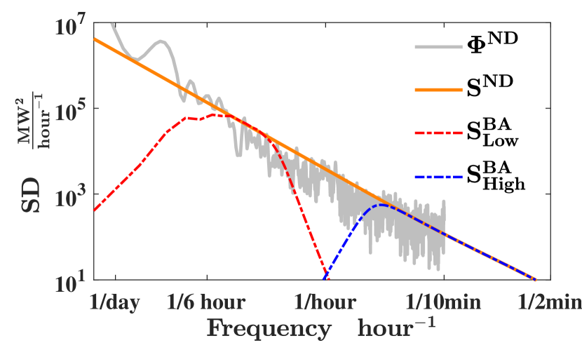
Figure 7: Empirical net demand SD , modeled SD for BPA’s net demand, and the two reference SD’s for the high and low frequency passband.

VI-B Meeting the BA’s needs with large buildings

In this scenario we consider a homogeneous collection of large commercial buildings. The idea is to illustrate how many of these large commercial buildings would be required to meet the grids needs as a function of frequency. To do this, the two reference SDs obtained from the previous section are projected (by solving (38)) onto the same ensemble constraint set with a varying number of large commercial buildings.

First, we show the results for $n=15000$ large commercial buildings in Figure 7. For the reference SD with high passband, the loads are able to meet the requirements of the grid, with an aggregate power and energy capacity index of $\zeta^{P}\approx 100\%$ and $\zeta^{E}\approx 100\%$. However, for the reference SD with low passband the loads are unable to meet the grids needs, with an aggregate power and energy capacity index of $\zeta^{P}=43\%$ and $\zeta^{E}=26\%$.

For a varying number of loads the power and energy capacity index are recorded and plotted as a function of $n$ in Figure 10. These results indicate that the BA would require $\approx$ 5000 large commercial buildings in the higher passband and $\approx$ 32000 large commercial buildings for the low passband, to fulfill its needs. We also see that the BAs energy capacity requirement is met with fewer loads (compared to its power capacity requirement) at the higher frequency range. In the lower frequency range, this conclusion is reversed.

In summary, this numerical experiment suggests that the commercial HVAC systems considered here are more suitable to assist the grid by tracking signals with SD in the higher passband. If a BA wanted the commercial HVAC systems to track reference signals in the lower frequency range, than significantly more large commercial HVAC systems would be required.

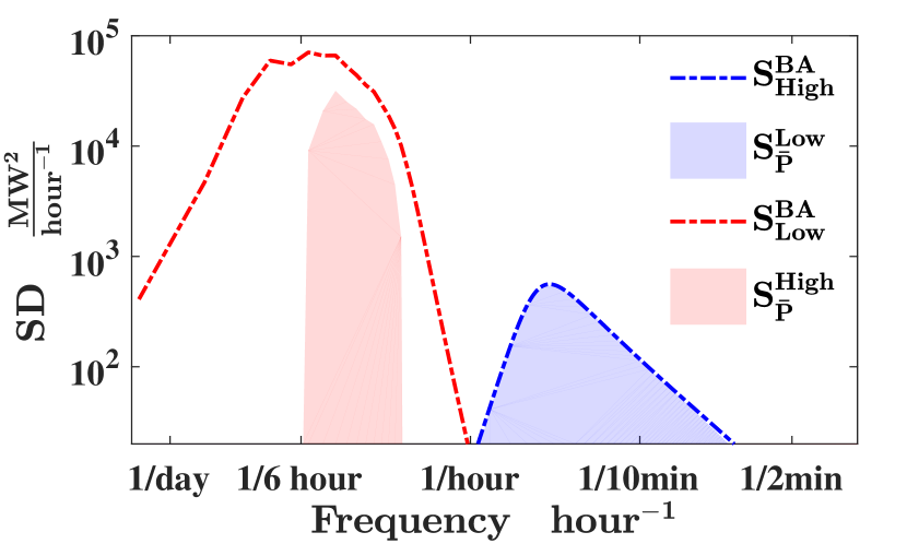
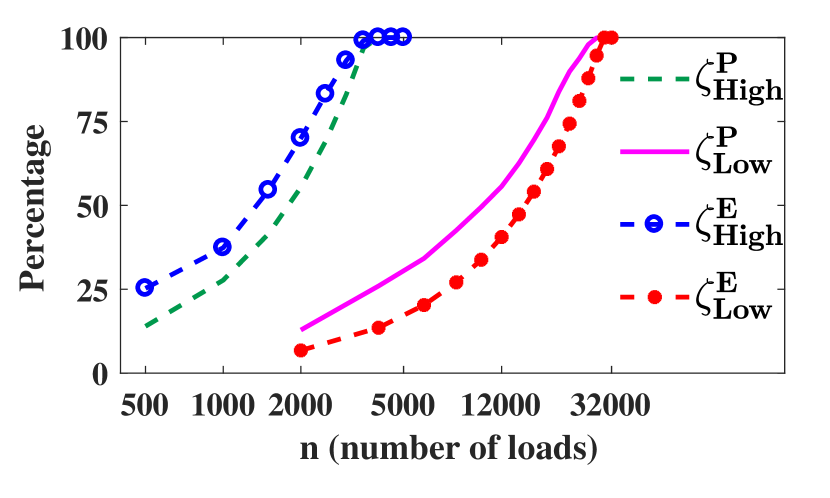
Figure 8: The two reference SDs and the ensembles SD (boundary of the shaded regions) obtained by solving (38) for a homogeneous collection of $n=15000$ loads.

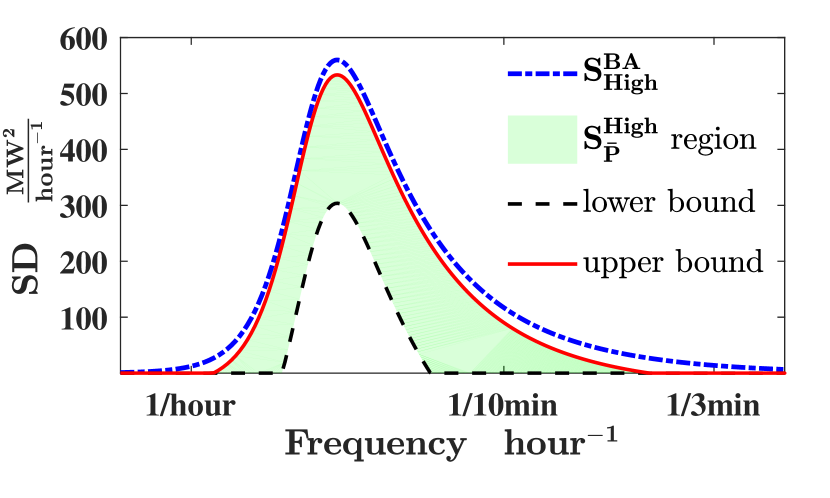
Figure 9: The aggregate power and energy capacity index for the two different reference SDs with a homogeneous collection of loads plotted against $n$.

Figure 10: The upper and lower bounds on the ensemble SD for a heterogeneous ensemble.

VI-C Effects of heterogeneity

We present a numerical experiment to illustrate the bounds in Corollary 2. We consider $n_{\text{bin}}=2$ bins with, $n_{1}=n_{S}=900$ small and $n_{2}=n_{L}=2100$ large commercial buildings. We solve the problem (38) twice, with the appropriate parameters detailed in Comment 1 for both times, so to obtain the upper and lower bounds in Corollary 2. This is done for the high passband in section VI-B and a low passband of $[\frac{1}{3}\text{1/hours},\frac{1}{15}\text{1/mins}]$.

The results of the high passband are shown in Figure 10, where ‘upper bound’ and ‘lower bound’ represent the upper and lower bounds in Corollary 2, respectively. Additionally, the shaded region in Figure 10 represents the region where the true ensemble SD lives. For this example, this gives us that the power capacity index is bounded as $17\%\leq\zeta^{P}\leq 69\%$ and the energy capacity index is bounded as $30\%\leq\zeta^{E}\leq 86\%$.

The results of the low passband are shown in Figure 11, where the outline of the shaded green regions represent the bounds in Corollary 2. Interestingly, the small and large buildings separate on the frequency axis. The large buildings cover the lower frequency components, whereas the small buildings cover the higher frequency components.

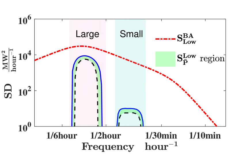
Figure 11: The upper and lower bounds on the ensemble SD for a heterogeneous ensemble with low passband.

VII Summary and conclusion

Our characterization of virtual energy storage capacity of flexible loads allows a balancing authority to quantify which loads can contribute how much to mitigating supply demand mismatch. In contrast to past work, our method can be used for long term planning. The key insight is to characterize capacity through statistics of the reference signal rather than on specific instances of the signal. This framework also has another benefit: it enables us to define power and energy capacity of virtual energy storage in language of real energy storage: kW’s and kWh’s.

An open problem is to extend the framework to non-stationary statistics of the grid’s demand-supply mismatch and/or loads’ demand deviation. Another open problem is the extension to the case of on/off loads. A key challenge for on/off loads will be to characterize their cycling constraint. Another avenue for future work is to consider a time of life QoS of the flexible load.

References

- [1] P. Barooah, Smart Grid Control: An Overview and Research Opportunities. Springer Verlag, 2019, ch. Virtual energy storage from flexible loads: distributed control with QoS constraints, pp. 99–115.
- [2] N. J. Cammardella, R. W. Moye, Y. Chen, and S. P. Meyn, “An energy storage cost comparison: Li-ion batteries vs Distributed load control,” in 2018 Clemson University Power Systems Conference (PSC), Sep. 2018, pp. 1–6.
- [3] A. Coffman, A. Bušić, and P. Barooah, “A study of virtual energy storage from thermostatically controlled loads under time-varying weather conditions,” in 5th International Conference on High Performance Buildings, July 2018, pp. 1–10.
- [4] M. Liu, S. Peeters, D. S. Callaway, and B. J. Claessens, “Trajectory tracking with an aggregation of domestic hot water heaters: Combining model-based and model-free control in a commercial deployment,” IEEE Transactions on Smart Grid, 2019.
- [5] H. Hao, A. Kowli, Y. Lin, P. Barooah, and S. Meyn, “Ancillary service for the grid via control of commercial building HVAC systems,” in American Control Conference, June 2013, pp. 467–472.
- [6] A. Aghajanzadeh and P. Therkelsen, “Agricultural demand response for decarbonizing the electricity grid,” Journal of Cleaner Production, vol. 220, pp. 827 – 835, 2019.
- [7] Y. Chen, A. Bušić, and S. Meyn, “State estimation for the individual and the population in mean field control with application to demand dispatch,” IEEE Transactions on Automatic Control, vol. 62, no. 3, pp. 1138–1149, March 2017.
- [8] Z. E. Lee, Q. Sun, Z. Ma, J. Wang, J. S. MacDonald, and K. Max Zhang, “Providing Grid Services With Heat Pumps: A Review,” ASME Journal of Engineering for Sustainable Buildings and Cities, vol. 1, no. 1, 01 2020, 011007.
- [9] H. Hao, B. M. Sanandaji, K. Poolla, and T. L. Vincent, “Aggregate flexibility of thermostatically controlled loads,” IEEE Transactions on Power Systems, vol. 30, no. 1, pp. 189–198, Jan 2015.
- [10] H. Hao, D. Wu, J. Lian, and T. Yang, “Optimal coordination of building loads and energy storage for power grid and end user services,” IEEE Transactions on Smart Grid, vol. PP, no. 99, pp. 1–1, 2017.
- [11] A. Coffman, N. Cammardella, P. Barooah, and S. Meyn, “Aggregate capacity of TCLs with cycling constraints,” arXiv preprint arXiv:1909.11497, 2019.
- [12] R. Yin, E. C. Kara, Y. Li, N. DeForest, K. Wang, T. Yong, and M. Stadler, “Quantifying flexibility of commercial and residential loads for demand response using setpoint changes,” Applied Energy, vol. 177, pp. 149 – 164, 2016.
- [13] H. Hao, J. Lian, K. Kalsi, and J. Stoustrup, “Distributed flexibility characterization and resource allocation for multi-zone commercial buildings in the smart grid,” in 2015 54th IEEE Conference on Decision and Control (CDC), Dec 2015, pp. 3161–3168.
- [14] J. T. Hughes, A. D. Domínguez-García, and K. Poolla, “Virtual battery models for load flexibility from commercial buildings,” in 2015 48th Hawaii International Conference on System Sciences, Jan 2015, pp. 2627–2635.
- [15] S. Kundu, K. Kalsi, and S. Backhaus, “Approximating flexibility in distributed energy resources: A geometric approach,” in 2018 Power Systems Computation Conference (PSCC), June 2018, pp. 1–7.
- [16] F. Lin and V. Adetola, “Flexibility characterization of multi-zone buildings via distributed optimization,” in 2018 Annual American Control Conference (ACC), June 2018, pp. 5412–5417.
- [17] P. Barooah, A. Bušić, and S. Meyn, “Spectral decomposition of demand side flexibility for reliable ancillary service in a smart grid,” in 48th Hawaii International Conference on Systems Science (HICSS), January 2015, invited paper.
- [18] A. Coffman, Z. Guo, and P. Barooah, “A spectral characterization of aggregate capacity of flexible loads for grid support,” in American Control Conference, July 2020, accepted.
- [19] E. M. Krieger, “Effects of variability and rate on battery charge storage and lifespan,” Ph.D. dissertation, Princeton University, 2013.
- [20] J. Apt, “The spectrum of power from wind turbines,” Journal of Power Sources, vol. 169, no. 2, pp. 369 – 374, 2007.
- [21] Y. Lin, P. Barooah, S. Meyn, and T. Middelkoop, “Experimental evaluation of frequency regulation from commercial building HVAC systems,” IEEE Transactions on Smart Grid, vol. 6, no. 2, pp. 776 – 783, 2015.
- [22] B. Kirby, “Ancillary services: Technical and commercial insights,” 2007, prepared for Wärtsilä North America Inc.
- [23] S. Huang and D. Wu, “Validation on aggregate flexibility from residential air conditioning systems for building-to-grid integration,” Energy and Buildings, vol. 200, pp. 58 – 67, 2019.
- [24] B. Hajek, Random processes for engineers. Cambridge university press, 2015.
- [25] M. Grant and S. Boyd, “CVX: Matlab software for disciplined convex programming, version 1.21,” http://cvxr.com/cvx, Feb. 2011.