Linear Instability of the Charged Massless Scalar Perturbation in Regularized 4D Charged Einstein-Gauss-Bonnet Anti de-Sitter Black Hole

Abstract

We study the linear instability of the charged massless scalar perturbation in regularized 4D charged Einstein-Gauss-Bonnet-AdS black holes by exploring the quasinormal modes. We find that the linear instability is triggered by superradiance. The charged massless scalar perturbation becomes more unstable when increasing the Gauss-Bonnet coupling constant or the black hole charge. Meanwhile, decreasing the AdS radius will make the charged massless scalar perturbation more stable. The stable region in parameter space $(\alpha,Q,\Lambda)$ is given. Moreover, we find that the charged massless scalar perturbation is more unstable for larger scalar charge. The modes of multipoles are more stable than that of the monopole.

I Introduction

The perturbations of black holes are powerful probes to disclose the stability of the black holes and have been studied intensively for decades. The linear (in)stability of the black hole can be characterized by the quasi-normal modes (QNMs). If the imaginary part of the QNMs are positive, the perturbation amplitude will grow exponentially and implies instability. The QNMs provide the finger-prints of black holes and are related to the gravitational wave observations Konoplya2011 . In four-dimensional spacetime, the black holes, such as the Schwarzschild black holes, Reissner–Nordström (RN) black holes and Kerr black holes, are stable under neutral scalar, electromagnetic field or gravitational perturbations in general Konoplya2011 , regardless of whether the black holes are in asymptotic flat, de Sitter (dS) or anti-dS (AdS) spacetimes. However, the four-dimensional black holes can be unstable provided superradiance occurs Brito2015 ; Zhu2014 ; Zhang2014 . The perturbations in higher dimensional spacetimes and alternative theories of gravity have also attracted a lot of attentions Li2019RNdS .

Recently, a regularized four-dimensional Einstein-Gauss-Bonnet (EGB) gravity theory was proposed Glavan20192019a , in which the Gauss-Bonnet coupling constant was rescaled with $\alpha\to\alpha/(D-4)$ in the limit $D\to 4$ and novel black hole solutions were found Fernandes2003 ; 4DEGBSolutions . This has stimulated a lot of studies, as well as doubts Kobayashi2004 ; Aoki2020 ; 4DStability ; Zhang2020Super ; Liu2020 ; 4DEGBShadow ; 4DEGBThermo ; 4DEGBOthers . Fortunately, some proposals have been raised to circumvent the issues of the regularized 4D EGB gravity, including adding an extra degree of freedom to the theory Kobayashi2004 , or breaking the temporal diffeomorphism invariance Aoki2020 , where a well-defined theory can be formulated. The regularized black hole solutions can still be derived from these more rigorous routes. Thus it is worth to study the perturbations of these black hole solutions. In fact, the stability of the regularized four-dimensional black hole has been studied from many aspects 4DStability , of which most focused only on the neutral cases. We studied the charged massless scalar perturbations in the regularized 4D charged EGB black holes with asymptotic flat and dS spacetimes in Zhang2020Super ; Liu2020 , respectively. It was found that the charged massless scalar perturbations in asymptotic flat spacetime are always stable, while those in asymptotic dS spacetime suffer from a new kind of test field instability where not all the modes satisfying the superradiant condition are unstable.

Since the boundary conditions in AdS spacetime are different from those in asymptotically flat or dS spacetimes, it can be expected that the behaviors of perturbations on the black holes in AdS spacetime would be different from those in flat or dS spacetime. Thus we study the charged scalar perturbation in the regularized 4D charged black hole in AdS spacetime in this paper. We find that the asymptotic iteration method used in Zhang2020Super ; Liu2020 does not work well here. Instead, we adopt another numerical method to calculate the frequencies of the perturbations. The QNMs are worked out as a generalized eigenvalue problem and the results are checked by the time-evolution method. We find that the charged massless scalar suffers from linear instability. However, unlike the dS case, all unstable modes here satisfy the superradiant condition. The effects of the Gauss-Bonnet coupling constant, the black hole charge, the scalar charge and cosmological constant were analyzed in detail.

This paper is organized as follows. In section II, we describe the regularized 4D charged EGB black hole in AdS spacetime and the parameter region allowing an event horizon of the black hole. In section III we elaborate the method to calculate the quasinormal modes of the charged scalar perturbation in regularized charged black hole. In sections IV, we study the effects of the Gauss-Bonnet coupling constant, the black hole charge, the scalar field charge and the cosmological constant on the QNMs in detail. Section V is our discussion.

II 4D Einstein-Gauss-Bonnet gravity

In spherically symmetric spacetime, the electrovacuum solution of the four-dimensional EGB gravity in AdS spacetime is given by Fernandes2003

$$ds^{2}=-f(r)dt^{2}+\frac{1}{f(r)}dr^{2}+r^{2}(d\theta^{2}+\sin^{2}\theta d\phi^{2}),$$ (1)

where the metric function

$$f(r)=1+\frac{r^{2}}{2\alpha}\left(1-\sqrt{1+4\alpha\left(\frac{M}{r^{3}}-\frac{Q^{2}}{r^{4}}{+}\frac{\Lambda}{3}\right)}\right),$$ (2)

and the gauge potential

$$A=-\frac{Q}{r}dt.$$ (3)

Here, $M,\,Q$ are the mass and charge of the black hole, respectively. In (2) the cosmological constant is $\Lambda=-3/l^{2}$, where $l$ is the cosmological radius. As $r\to\infty$, the solution approaches an asymptotic AdS spacetime if

$$\frac{1}{2\alpha}\left(1-\sqrt{1{+}\frac{4\alpha\Lambda}{3}}\right)>0.$$ (4)

This condition can be satisfied only for negative $\Lambda$ no matter $\alpha$ is positive or negative. When $\alpha\to 0$, the solution goes back to the RN-AdS black hole. Note that the solution (1) coincides formally with those obtained from conformal anomaly and quantum corrections Cai20019 and those from Horndeski theory Kobayashi2004 .

We fix the black hole event horizon $r_{+}=1$ in this paper. To ensure $f(r_{+})=0$, there should be $\alpha>-1/2$. The mass $M$ can be expressed as

$$M=\frac{1}{3}\left(3\alpha{-}\Lambda+3Q^{2}+3\right).$$ (5)

The parameter region that allows the existence of a black hole with positive Hawking temperature on the event horizon is determined by $f^{\prime}(r_{+})>0$. This leads to an inequality which is very similar to the case in dS spacetime Liu2020 .

$$Q^{2}+\alpha{+}\Lambda<1.$$ (6)

The region plot of the allowed parameter region is given in Fig. 1,

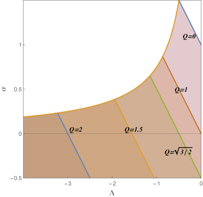
Figure 1: The parameter region that allows the existence of a black hole with metric function (2). The allowed region for a larger $Q$ is a subset of that for a smaller $Q$.

from which we can find that the allowed region (shaded region) shrinks when increasing $Q$. However, unlike the case in dS spacetime, the black hole charge $Q$ is unbounded in asymptotic AdS spacetime here.

III Quasinormal modes and numerical methods

We study the linear stability of a massless charged scalar perturbation $\psi$ in the black hole solution (1). It is known that fluctuations of order $O(\epsilon)$ in the scalar field in a given background induce changes in the spacetime geometry of order $O(\epsilon^{2})$ Brito2015 . To leading order, we can study the perturbations on the fixed background geometry that satisfies

$$D_{\mu}D^{\mu}\psi=0,$$ (7)

where $D_{\mu}\equiv\nabla_{\mu}-ieA_{\mu}$, and $e$ is the charge of the test scalar field.

It is more convenient to work under the ingoing Eddington-Finkelstein coordinate

$$v=t+r_{*},$$ (8)

when studying the time evolution of the perturbation. Here $r_{*}$ is the tortoise coordinate defined with $dr_{*}=dr/f$. In this coordinate, the line element becomes

$$ds^{2}=-fdv^{2}+2dvdr+r^{2}d\Omega^{2}_{2}.$$ (9)

The Maxwell field in Eddington-Finkelstein coordinates is

$$A=-\frac{Q}{r}dv,$$ (10)

where we get rid of the spatial component of the gauge field by a gauge transformation.

The equation of motion (7) is separable by taking the following form

$$\psi=\frac{\phi(v,r)Y_{lm}(\theta,\varphi)}{r},$$ (11)

where $Y_{lm}$ is the spherical harmonic function. Inserting (11) into (7) we have

$$f\partial_{r}^{2}\phi+f^{\prime}\partial_{r}\phi-2ieA_{v}\partial_{r}\phi-ieA^{\prime}_{v}\phi+2\partial_{v}\partial_{r}\phi+V(r)\phi=0,$$ (12)

where the prime ^′ denotes the derivative with respect to $r$, and the effective potential is

$$V(r)=-f^{\prime}(r)/r-l(l+1)/r^{2}.$$ (13)

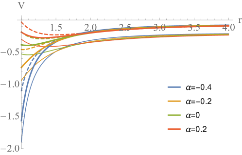
Figure 2: The effective potential when $l=0$. The thick lines for $Q=0.6,\Lambda={-}0.1$, the thin lines for $Q=0.6,\Lambda={-}0.3$, the dashed lines for $Q=0.8,\Lambda={-}0.1$.

We show the effective potential when $l=0$ in Fig. 2. When $Q$ and $\Lambda$ are fixed, the effective potential well becomes shallower as $\alpha$ increases. When $\Lambda$ and $\alpha$ are fixed (the thick lines and dashed lines), the effective potential well becomes shallower as $Q$ increases. When $Q$ and $\alpha$ are fixed (the thick lines and thin lines), the effective potential becomes deeper as $\Lambda$ increases. We will see that these behaviors of effective potential are related to the linear instability structure of the massless charged scalar perturbation on the black hole.

In order to implement the frequency analysis on (12), we consider the following mode

$$\phi(v,r)=\phi(r)e^{-i\omega v}.$$ (14)

Then equation (12) becomes

$$f\partial_{r}^{2}\phi+f^{\prime}\partial_{r}\phi-2ieA_{v}\partial_{r}\phi-ieA^{\prime}_{v}\phi-2i\omega\partial_{r}\phi+V(r)\phi=0.$$ (15)

A more convenient approach to implement the numerics is to work under $z\equiv r_{+}/r$ coordinate, such that we can solve the equation of motion in a bounded region $z\in[0,1]$. This coordinate has been widely adopted in solving gravitational background solutions and perturbations Lingbefore . Here the ingoing condition at horizon is satisfied by setting the time-dependent factor $e^{-i\omega v}$ and requiring a regular $\phi(r)$ near the horizon. The asymptotic AdS requires a vanishing $\phi(r)$ at the boundary, that can be realized by extracting $1/r$ from $\phi$.

The next step is to find the QNMs, i.e. the modes with complex frequency $\omega=\omega_{R}+i\omega_{I}$. When the imaginary part $\omega_{I}>0$, the perturbation amplitude grows exponentially with time. When the amplitude becomes large enough, the back reaction of the perturbation on the geometry can not be ignored and implies that the system may become unstable. However, at this stage, the linear approximation adopted in this paper is inadequate and the full nonlinear studies are required.

The radial equation (15) is generally hard to solve analytically, except for a few instances such as the pure (A)dS spacetimes and Nariai spacetime Konoplya2011 . Various numerical methods were developed to obtain the QNMs, such as the WKB method, perturbation method, and iteration methods qnmmethods .

Recently, a new method that re-casts the search for QNMs to a generalized eigenvalue problem by discretizing the equation of motion has been proposed newmethod . In this paper, we discretize the spatial coordinate with Gauss-Lobatto grid with $N$ collocation points. It has been shown that the Gauss-Lobatto grid is an efficient method for solving the eigenvalue problems Boyd:2001 . We examined this in our calculations and found that the Gauss-Lobatto collocation method requires significantly fewer points than the uniform collocation method to achieve the same accuracy. With the discretization, we arrive at a discretized version of (15),

$$\left(\mathcal{M}_{0}+\omega\mathcal{M}_{1}\right)\vec{\phi}=0,$$ (16)

where $\mathcal{M}_{0,1}$ are $N\times N$ complex-valued matrices and independent of $\omega$. The eigenvalues $\omega$ in (16) can be efficiently solved by Eigenvalues[-$\mathcal{M}_{0}$,$\mathcal{M}_{1}$] with Mathematica. Equivalently, one may also solve the roots of $\det\left(\mathcal{M}_{0}+\omega\mathcal{M}_{1}\right)=0$ to find the eigenvalues. Resultantly, a finite set $\{\omega\}$ with $N$ elements can be obtained, of which some are spurious QNMs. The results are reliable only if they are convergent when increasing the collocation density. The fundamental mode is the one with the largest imaginary part.

IV Results

We study the linear instability of the massless charged scalar field in 4D EGB model by showing the relation between the dominant QNMs and the system parameters. We first explore the effect of $\alpha,\,Q,\,\Lambda$ and $e$ on the QNMs, respectively. After that we study the comprehensive linear instability structure of the massless charged scalar perturbation by showing the stable region in the allowed parameter space.

IV.1 QNMs vs $\alpha$

In the asymptotic dS case, the effect of $\alpha$ on the linear instability depends on the specific values of $Q$ and $\Lambda$ Liu2020 . It is especially important to find out the role the GB coupling constant $\alpha$ plays in the linear instability structure of AdS case here.

As an example, we fix $\Lambda={-}2/3,\,e=1,\,l=0$ and demonstrate the QNMs vs $\alpha$ in Fig. 3. We can see that the real part of the fundamental mode $\omega_{R}$ decreases with $\alpha$ monotonically. By comparing the curves of different charges $Q$ we find that $\omega_{R}$ monotonically decreases with $Q$. Meanwhile, we can find that the imaginary part of the fundamental mode $\omega_{I}$ first decreases with $\alpha$ and then increases with $\alpha$. The imaginary part $\omega_{I}$ increases with $Q$, indicating that increasing $Q$ may lead to linear instability. However, in Fig. 3 where we have fixed $e=1$, the $\omega_{I}$ is always negative and no linear instability occurs.

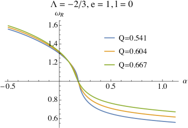
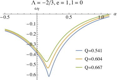
Figure 3: The left and the right plots are $\omega_{R}$ and $\omega_{I}$ of the fundamental modes vs $\alpha$ at $\Lambda={-}2/3,\,e=1,\,l=0$, respectively.

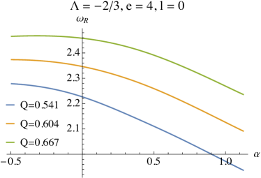
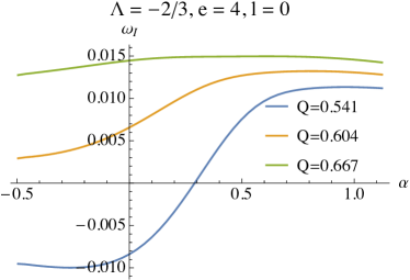
Figure 4: The left and the right plots are $\omega_{R}$ and $\omega_{I}$ vs $\alpha$ of the fundamental modes at $\Lambda={-}2/3,\,e=4,\,l=0$, respectively.

We show the fundamental modes vs $\alpha$ at larger scalar charge $e=4$ in Fig. 4. Apparently, the $\omega_{R}$ also monotonically decreases with $\alpha$, which is in accordance with that of the case when $e=1$. For the imaginary part, we find that when $Q$ is relatively small, $\omega_{I}$ first decreases with $\alpha$ and then increases with $\alpha$ (see the blue curve in the right plot of Fig. 4), this is similar to that of $e=1$. However, when $\alpha$ is relatively large, $\omega_{I}$ can become positive and lead to linear instability here. Therefore the linear instability occurs only at large enough value of perturbation charge $e$. For intermediate values of $Q$, we find that $\omega_{I}$ can increase with $\alpha$ monotonically. For large values of $Q$, the $\omega_{I}$ can decrease with $\alpha$ for relatively large $\alpha$. In addition to that, we can see that both $\omega_{R}$ and $\omega_{I}$ increases with $Q$ for $e=4$. The more comprehensive dependence of the linear instability on the scalar charge $e$ is given in subsection IV.4.

From the viewpoint of the effective potential shown in Fig. 2, increasing $\alpha$ makes the effective potential well shallower. An effective potential barrier appears near the horizon when $\alpha$ is large enough. The scalar perturbation is harder to be absorbed by the black hole and can accumulate in the effective potential well. As a consequence, the massless charged scalar field tends to be unstable as $\alpha$ increases and the imaginary part of the frequency $\omega_{I}$ tends to be positive.

It has been shown modes of $l>0$ are usually more stable than those of $l=0$ Liu2020 . In present model, similar phenomenon can also be observed. We show the fundamental modes vs $\alpha$ at $e=4,\,l=1$ in Fig. 5. Comparing Fig. 4 and Fig. 5 we see that $\omega_{I}$ for $l=1$ is smaller than that of $l=0$, which implies that $l=1$ perturbation mode is indeed more stable than that of $l=0$ mode. For the real part of the fundamental mode, we find that $\omega_{R}$ for $l=1$ is larger than that of $l=0$, which corresponds to a more rapidly oscillating mode.

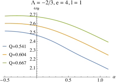
Figure 5: Fundamental modes vs $\alpha$ at $\Lambda={-}2/3,\,e=4,\,l=1$, where the left and the right plots are the real part and imaginary part of the fundamental modes, respectively.

In this subsection, we find that increasing the coupling constant $\alpha$ can lead to linear instability, and this instability occurs only at large enough perturbation charge $e$. Moreover, the stability is enhanced when increasing the degree $l$.

IV.2 QNMs vs $Q$

In the previous subsection, we find that $\omega_{I}$ increases with $Q$ by comparing several examples at different $Q$’s (Fig. 3 and Fig. 4). Here we explore more comprehensive relationship between the QNMs and the black hole charge $Q$. In Fig. 6 we show the dependence of QNMs on $Q$ when $\alpha=-\frac{99}{200},\,e=1,\,l=0$ as an example. We find that both $\omega_{R}$ and $\omega_{I}$ increase with $Q$. Especially, $\omega_{I}$ can become positive when increasing $Q$, this means that increasing $Q$ will render the system more unstable and more oscillating. This is in accordance with the observations in the previous subsection.

Comparing the thick lines and dashed lines in Fig. 2, we see that increasing the black hole charge makes the effective potential at the horizon larger. It is harder to absorb the perturbations by black holes with larger $Q$. The perturbations can be trapped more easily in the effective potential well. Thus increasing $Q$ makes the system more unstable.

Also, by comparing the data at different values of $\Lambda$ we find that $\omega_{R}$ decreases when increasing $\Lambda$, while $\omega_{I}$ increases when increasing $\Lambda$. This phenomenon suggests that decreasing $\Lambda$ will make the charged massless scalar perturbation more stable and less oscillating.

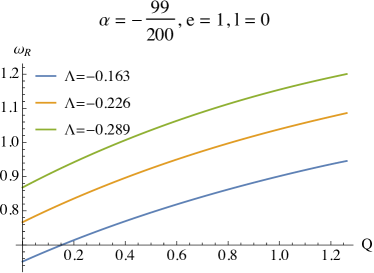
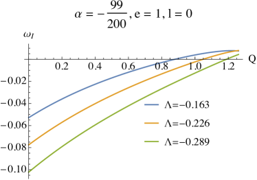
Figure 6: Fundamental modes vs $Q$ at $\alpha=-99/200,\,e=1,\,l=0$, where the left and the right plots are the real part and imaginary part of the fundamental modes, respectively.

IV.3 QNMs vs $\Lambda$

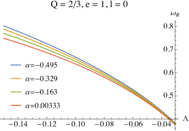
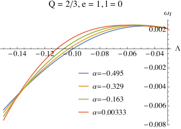
Figure 7: Fundamental modes vs $\Lambda$ at $Q=1/10,\,e=1,\,l=0$, where the left and the right plots are the real part and imaginary part of the fundamental modes, respectively.

We show the QNMs vs $\Lambda$ when $Q=1/10,\,e=1,\,l=0$ in Fig. 7. From the left plot we see that $\omega_{R}$ monotonically decreases with $\Lambda$. For the imaginary part, when $|\Lambda|$ is relatively small, $\omega_{I}$ is positive and decreases with $\Lambda$, the system is always unstable . However, when $\Lambda$ further decreases, $\omega_{I}$ reaches its local maximum and then starts to decrease. When decreasing the $\Lambda$ even further, $\omega_{I}$ becomes negative and the system becomes stable. This again certifies the observations in the last subsection that the system becomes more stable and more rapidly oscillating when decreasing $\Lambda$. From the potential behaviors in Fig. 2, we see that decreasing $\Lambda$ makes effective potential well deeper. The perturbations can be trapped more easily by black holes with larger $\Lambda$. Thus decreasing $\Lambda$ makes the system more stable. Observing the points where $\omega_{I}=0$ we can also find that the system becomes more stable when increasing $\alpha$.

IV.4 QNMs vs $e$

In this subsection, we systematically study the relationship between the linear instability of the charged massless scalar field and the scalar charge $e$. In principle, the scalar charge $e$ can be either positive or negative. However, here the linear instability structure with negative charge $-|e|$ is the same as that of the positive charge $|e|$. Inserting the Maxwell field (10) into (12), we have

$$f\partial_{r}^{2}\phi+f^{\prime}\partial_{r}\phi-2ieQ\partial_{r}\phi/r-ieQ\phi/r^{2}+2\partial_{v}\partial_{r}\phi+V(r)\phi=0,$$ (17)

from which we find that $e$ always appears in pairs with $iQ$, and the other terms contain only $Q^{2}$. Accordingly, by separating the real part and imaginary part, the discrete eigenvalue equation (16) can be decomposed into the following form

$$\left[({\mathcal{M}}^{R}_{0}+i\omega_{I}{\mathcal{M}}_{1})+i({\mathcal{M}}^{I}_{0}-i\omega_{R}{\mathcal{M}}_{1})\right]\vec{\phi}=0.$$ (18)

Here ${\mathcal{M}}_{1}$ is a pure imaginary matrix because $\omega$ always comes in pairs with $i$ in (15) and $\partial_{r}$ only contributes a real-valued differential matrix. The conjugate of (18) becomes,

$$\left[({\mathcal{M}}^{R}_{0}+i\omega_{I}{\mathcal{M}}_{1})+i(-{\mathcal{M}}^{I}_{0}+i\omega_{R}{\mathcal{M}}_{1})\right]\vec{\phi}^{*}=0.$$ (19)

Consequently, performing ${\mathcal{M}}^{I}_{0}\to-{\mathcal{M}}^{I}_{0}$, which can result from performing $e\to-e$ since $\mathcal{M}^{I}_{0}$ is linear in $e$, we obtain a root $-\omega^{*}=-\omega_{R}+i\omega_{I}$. Therefore, we proved that when we perform $e\to-e$, the imaginary part of the QNMs will be the same, while the real part of the QNMs becomes the opposite of itself. We have also verified this result in our numerics. Fig. 8 shows the properties of the QNMs when changing the sign of $e$. Therefore, we can safely focus on positive $e$ to reveal the linear instability. Next, we present the explicit effect of the perturbation charge $e$ on the QNMs, along $\alpha,\,Q,\,\Lambda$, respectively.

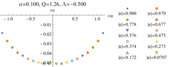
Figure 8: The fundamental modes for different values of $e$. Each color or marker corresponds to a pair of $e$’s with an absolute value $|e|$, where the left hand side is $e=-|e|$ and the right hand side $e=|e|$.

The phenomena are qualitatively the same along $\alpha,\,Q,\,\Lambda$, that we demonstrate in Fig. 9. The $\omega_{I}$ increases with the increase of $e$ for arbitrary parameter. Next, we study the comprehensive instability structure by locating the critical surfaces separating the stable regions and unstable regions.

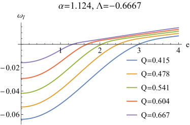
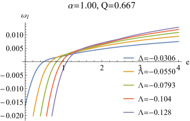
Figure 9: From top to bottom, the QNMs vs $e$ at several different values of $Q,\,\alpha,\,\Lambda$, respectively.

IV.5 Stable Region

In order to determine the linear instability structure, we need to locate the critical surfaces on which $\omega_{I}$ vanishes. By searching the parameter space subject to the allowed region, we show a comprehensive stable region in Fig. 10 when $e=1,\,l=0$. The linear instability structure in parameter space $(\alpha,\,Q,\,\Lambda)$ are much simpler than that of the dS case Liu2020 . Fig. 10 suggests that system becomes more unstable when increasing $Q$ or $\alpha$, while increasing $\Lambda$ will make the system more stable. Comparing the solid curves $(e=1)$ and the dashed curves $(e=1.263)$ in Fig. 10, we find that the stable region indeed shrinks when increasing $e$. These are consistent with the results from previous subsections.

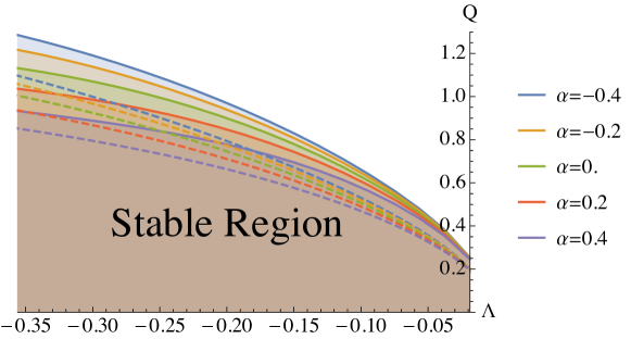
Figure 10: The shaded regions are the stable regions at $e=1,\,l=0$, where each solid line corresponds to different values of $\alpha$ marked by the plot legends. The dashed lines are the critical lines for $e=1.263$, with $\alpha$ specified by the plot legends with the same color.

In the unstable region, we find that the real part of the fundamental modes frequencies of the massless charged scalar perturbation always satisfy the superradiance condition,

$$\frac{eQ}{r_{+}}>\omega_{R}.$$ (20)

In the stable region, the fundamental modes violate the above condition. This suggests that the linear instability from the QNM analysis is triggered by the superradiance instability. We list the QNMs at several critical points of the linear stability/instability transitions in Table 1, from which we can find that $eQ/r_{+}$ matches perfectly with the real part of the QNMs. Remind that in the dS case Liu2020 , the superradiance condition is the necessary but not sufficient condition for linear instability.

$\alpha$	$\Lambda$	$\frac{eQ}{r_{+}}$	$\omega$
$-0.4$	${-}0.337501$	${1.25639}$	${1.25639}+3.56078\times 10^{-7}i$
$-0.4$	${-}0.356251$	${1.28588}$	${1.28588}+8.14388\times 10^{-8}i$
$-0.2$	${-}0.337501$	${1.19356}$	${1.19355}+6.51663\times 10^{-7}i$
$-0.2$	${-}0.356251$	${1.21722}$	${1.21722}+4.84345\times 10^{-7}i$
$0.$	${-}0.337501$	${1.11398}$	${1.11398}-1.03083\times 10^{-6}i$
$0.$	${-}0.356251$	${1.13248}$	${1.13248}+1.60832\times 10^{-7}i$
$0.2$	${-}0.337501$	${1.02122}$	${1.02122}+7.20995\times 10^{-7}i$
$0.2$	${-}0.356251$	${1.03673}$	${1.03673}-3.68094\times 10^{-7}i$
$0.4$	${-}0.337501$	${0.919189}$	${0.919191}-5.03797\times 10^{-7}i$
$0.4$	${-}0.356251$	${0.933379}$	${0.933378}+1.42506\times 10^{-7}i$

Table 1: The fundamental modes at several critical points of the stability-instability transitions corresponding to Fig. 10.

IV.6 Time Integral

In this subsection, we directly implement the time-evolution, i.e., the time integral, of the perturbation field subject to (12). This analysis is important since it can reveal the linear instability structure in a more transparent manner. Meanwhile, it can work as a double check of the frequency analysis.

On the event horizon, we set the ingoing boundary condition. On the AdS boundary, we set $\phi(v,z=0)=0$ as required by the asymptotic AdS geometry. We discretize the spatial direction $z$ with Gauss-Lobatto collocation; while on time direction $v$, we march with the fourth order Runge-Kutta method, which has been widely adopted in time evolution problem. Given certain initial profile of the scalar perturbation $\phi$, the time-evolution can be obtained.

We show the time evolution of the $\phi$ near critical lines in Fig. 11, where we can see that the $\log|\phi|$ quickly becomes linear with $t$. It seems like all curves are flat, but they have very small slope, as can be seen from Table. 1. The small slope (either positive or negative) is expected since the system is near the critical line for the linear stability/instability transition.

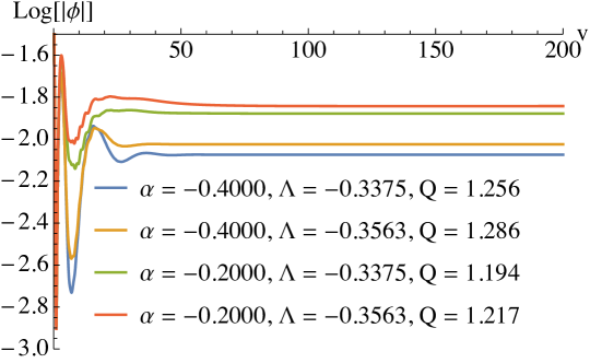
Figure 11: The time integral of the perturbation $\phi(z=0.997,v)$ at different values of $\alpha,\Lambda,Q$ in the critical region. The initial profile of $\phi$ is $\phi(z,v=0)=e^{-5{(z-0.5)^{2}}}$. The time step is $\Delta v=0.0025$, and we evolve the perturbation to $v=200$.

We worked out $\partial_{t}\log|\phi|$ at $t=1000$, which is large enough to obtain stable slopes, i.e., the imaginary part of the dominant modes. Apparently, the slopes should match the results from the frequency analysis. In our numerics we find that they are in good match indeed. For example, the slope for $\alpha=-0.2000,\Lambda={-}0.3375,Q=1.194$ is $6.50994\times 10^{-7}$, where the $\omega_{I}=6.51663\times 10^{-7}$, as we can see from the third row in Table. 1. These are results near the critical lines, where the numerical precision is hard to control since the $\omega_{I}$ tends to vanish in critical regions. For regions away from the critical region, the time integral results match much better with those of the frequency analysis. We show some examples in Fig. 12. For the unstable modes, the slopes are positive; while for stable modes, the slopes are negative. The stabilized slopes do not depend on the specific initial profiles and the locations where we sample the scalar perturbations $\phi$. The above results show that our frequency analysis is robust.

Figure 12: The time integral of the perturbation $\phi(z=0.997,v)$ at different values of $\alpha,\Lambda,Q$ away from the critical region. The initial profile of $\phi$ is $\phi(z,v=0)=e^{-5{(z-0.5)^{2}}}$. The time step is $\Delta v=0.01$, and we evolve the perturbation to $v=700$.

V Discussion

We studied the linear instability of the charged massless scalar field in regularized 4D charged EGB model with asymptotic AdS boundary by examining the QNMs. The detailed linear instability structure of the model was studied by the QNMs vs system parameters $(\alpha,\,Q,\,\Lambda)$ and the scalar charge $e$. We find that the system is unstable against the charged massless scalar when increasing $\alpha$ and $Q$, or increasing $\Lambda$. These phenomena have been explained intuitively from the viewpoint of the effective potential. Also, we find that the system is more unstable for larger perturbation charge $e$ and smaller values of $l$. Moreover, the superradiance condition starts to be satisfied across the critical line where linear instability occurs. Time evolution of the perturbation field matches perfectly with the results from the frequency analysis.

Finally, we point out several topics worthy of further study. First, it would be interesting to explore the linear instability structure of the present theory with a massive perturbation. In addition to the scalar perturbation, it is also desirable to reveal the linear instability for tensor perturbations and Dirac fields. Moreover, the instability of the background metric is also worthy of further studies.

References

-
(1)
E. Berti, V. Cardoso, A. O. Starinets, Quasinormal
modes of black holes and black branes, Class.Quant.Grav. 26 (2009)
163001, arXiv:0905.2975 [gr-qc].
R. A. Konoplya, A. Zhidenko, Quasinormal modes of black holes: From astrophysics to string theory, Rev.Mod.Phys. 83 (2011) 793-836, arXiv:1102.4014 [gr-qc]. -
(2)
P. Pani, E. Berti, L. Gualtieri, Gravitoelectromagnetic
Perturbations of Kerr-Newman Black Holes: Stability and Isospectrality
in the Slow-Rotation Limit. Phys. Rev. Lett. 110, 241103 (2013). arXiv:1304.1160
[gr-qc].
Dias O.J.C., Godazgar M., Santos J.R. Linear Mode Stability of the Kerr-Newman Black Hole and Its Quasinormal Modes. Phys. Rev. Lett. 114, 151101 (2015), arXiv:1501.04625 [gr-qc]. - (3) R. Brito, V. Cardoso, P. Pani, Superradiance – the 2020 Edition, Lect.Notes Phys. 906 (2015) pp.1-237, arXiv:1501.06570 [gr-qc].
-
(4)
Z. Zhu, S.-J. Zhang, C. E. Pellicer, B. Wang, Elcio
Abdalla, Stability of Reissner-Nordström black hole in de Sitter background
under charged scalar perturbation, Phys.Rev. D90 (2014) no.4, 044042,
Addendum: Phys.Rev. D90 (2014) no.4, 049904, arXiv:1405.4931 [hep-th].
R. A. Konoplya, A. Zhidenko, Charged scalar field instability between the event and cosmological horizons, Phys. Rev. D 90, 064048 (2014), arXiv:1406.0019 [hep-th]. - (5) C. Y. Zhang, S. J. Zhang, and B. Wang, Superradiant instability of Kerr-de Sitter black holes in scalar-tensor theory, JHEP 08 (2014) 011. arXiv:1405.3811.
-
(6)
R. A. Konoplya and A. Zhidenko, instability of higher dimensional charged black holes in
the de-Sitter world, Phys. Rev. Lett. 103 (2009) 161101, arXiv:0809.2822 [hep-th].
R. A. Konoplya and A. Zhidenko, instability of D-dimensional extremally charged Reissner Nordstrom(-de Sitter) black holes: Extrapolation to arbitrary D, Phys. Rev. D 89, no. 2, 024011 (2014) [arXiv:1309.7667 [hep-th]].
C. Y. Zhang, S. J. Zhang, and B. Wang, Charged scalar perturbations around Garfinkle–Horowitz–Strominger black holes, Nucl. Phys. B899, 37 (2015). arXiv:1501.03260.
C. Y. Zhang, S. J. Zhang, D. C. Zou, B. Wang, Charged scalar gravitational collapse in de Sitter spacetime, Phys.Rev. D93 (2016) no.6, 064036, arXiv:1512.06472 [gr-qc].
M. A. Cuyubamba, R. A. Konoplya and A. Zhidenko, Quasinormal modes and a new instability of Einstein-Gauss-Bonnet black holes in the de Sitter world, Phys.Rev. D 93 (2016) no.10, 104053, arXiv:1604.03604 [gr-qc]
C.-Y. Zhang, P.-C. Li, B. Chen, Greybody factors for Spherically Symmetric Einstein-Gauss-Bonnet-de Sitter black hole, Phys.Rev. D97 (2018) no.4, 044013, arXiv:1712.00620.
M. F. Wondrak, P. Nicolini and J. W. Moffat, Superradiance in Modified Gravity (MOG), JCAP 1812, 021 (2018) [arXiv:1809.07509 [gr-qc]].
P.-C. Li, C.-Y. Zhang, B. Chen, The Fate of instability of de Sitter Black Holes at Large D, JHEP 1911 (2019) 042, arXiv:1909.02685 [hep-th].
M. Khodadi, A. Talebian and H. Firouzjahi, Black Hole Superradiance in f(R) Gravities, arXiv:2002.10496 [gr-qc].
P.-C. Li, C.-Y. Zhang, Hawking radiation for scalar fields by Einstein-Gauss-Bonnet-de Sitter black holes, Phys.Rev. D99 (2019) no.2, 024030, arXiv:1901.05749 [hep-th]. - (7) D. Glavan and C. Lin, Einstein-Gauss-Bonnet gravity in 4-dimensional space-time, Phys. Rev. Lett. 124, no. 8, 081301 (2020), arXiv:1905.03601 [gr-qc].
- (8) P. G. S. Fernandes, Charged Black Holes in AdS Spaces in 4D Einstein Gauss-Bonnet Gravity, Phys.Lett.B 805 (2020) 135468. arXiv:2003.05491 [gr-qc].
-
(9)
A. Casalino, A. Colleaux, M. Rinaldi and
S. Vicentini, Regularized Lovelock gravity, arXiv:2003.07068 [gr-qc].
R. A. Konoplya and A. Zhidenko, Black holes in the four-dimensional Einstein-Lovelock gravity, Phys.Rev.D 101 (2020) 8, 084038. arXiv:2003.07788 [gr-qc].
R. A. Konoplya and A. Zhidenko, BTZ black holes with higher curvature corrections in the 3D Einstein-Lovelock theory, arXiv:2003.12171 [gr-qc].
S. W. Wei, Y. X. Liu, Testing the nature of Gauss-Bonnet gravity by four-dimensional rotating black hole shadow, arXiv:2003.07769 [gr-qc].
R. Kumar, S. G. Ghosh, Rotating black holes in the novel 4D Einstein-Gauss-Bonnet gravity, JCAP 07 (2020) 07, 053. arXiv:2003.08927 [gr-qc].
S. G. Ghosh and S. D. Maharaj, Radiating black holes in the novel 4D Einstein-Gauss-Bonnet gravity, Phys.Dark Univ. 30 (2020) 100687. arXiv:2003.09841 [gr-qc].
S. G. Ghosh and R. Kumar, Generating black holes in the novel Einstein-Gauss-Bonnet gravity, arXiv:2003.12291 [gr-qc].
A. Kumar and S. G. Ghosh, Hayward black holes in the novel Einstein-Gauss-Bonnet gravity, arXiv:2004.01131 [gr-qc].
A. Kumar and R. Kumar, Bardeen black holes in the novel Einstein-Gauss-Bonnet gravity, arXiv:2003.13104 [gr-qc].
D. D. Doneva and S. S. Yazadjiev, Relativistic stars in 4D Einstein-Gauss-Bonnet gravity, arXiv:2003.10284 [gr-qc].
P. Liu, C. Niu, X. Wang, C. Y. Zhang, Thin-shell wormhole in the novel 4D Einstein-Gauss-Bonnet theory, arXiv:2004.14267 [gr-qc].
K. Jusufi, A. Banerjee, S. G. Ghosh, Wormholes in 4D Einstein-Gauss-Bonnet Gravity, Eur.Phys.J.C 80 (2020) 8, 698. arXiv:2004.10750 [gr-qc].
L. Ma, H. Lu, Vacua and Exact Solutions in Lower-D Limits of EGB, arXiv:2004.14738 [gr-qc].
H. Lu, P. Mao, Asymptotic structure of Einstein-Gauss-Bonnet theory in lower dimensions, arXiv:2004.14400 [hep-th].
K. Yang, B. M. Gu, S. W. Wei, Y. X. Liu, Born-Infeld Black Holes in novel 4D Einstein-Gauss-Bonnet gravity, arXiv:2004.14468 [gr-qc].
S. G. Ghosh, S. D. Maharaj, Noncommutative inspired black holes in regularised 4D Einstein-Gauss-Bonnet theory, arXiv:2004.13519 [gr-qc]. -
(10)
T. Kobayashi, Effective scalar-tensor description
of regularized Lovelock gravity in four dimensions, JCAP 07 (2020) 013. arXiv:2003.12771
[gr-qc].
H. Lu and Y. Pang, Horndeski Gravity as Limit of Gauss-Bonnet, Phys.Lett.B 809 (2020) 135717. arXiv:2003.11552.
P. G. S. Fernandes, P. Carrilho, T. Clifton, D. J. Mulryne, Derivation of Regularized Field Equations for the Einstein-Gauss-Bonnet Theory in Four Dimensions, Phys.Rev.D 102 (2020) 2, 024025. arXiv:2004.08362.
Robie A. Hennigar, David Kubiznak, Robert B. Mann, Christopher Pollack, On Taking the limit of Gauss-Bonnet Gravity: Theory and Solutions, JHEP 07 (2020) 027. arXiv:2004.09472 [gr-qc].
S. Mahapatra, A note on the total action of 4D Gauss-Bonnet theory, arXiv:2004.09214.
W. Y. Ai, A note on the novel 4D Einstein-Gauss-Bonnet gravity, Commun.Theor.Phys. 72 (2020) 9, 095402. arXiv:2004.02858.
F. W. Shu, Vacua in novel 4D Einstein-Gauss-Bonnet Gravity: pathology and instability? arXiv:2004.09339 [gr-qc]. -
(11)
K. Aoki, M. A. Gorji and S. Mukohyama, A consistent theory of EinsteinGaussBonnet gravity, [arXiv:2005.03859 [gr-qc]].
K. Aoki, M. A. Gorji and S. Mukohyama, Cosmology and gravitational waves in consistent Einstein-Gauss-Bonnet gravity, [arXiv:2005.08428 [gr-qc]] -
(12)
R. A. Konoplya and A. F. Zinhailo, Quasinormal
modes, stability and shadows of a black hole in the novel 4D Einstein-Gauss-Bonnet
gravity, arXiv:2003.01188 [gr-qc].
R. A. Konoplya and A. Zhidenko, (In)stability of black holes in the 4D Einstein-Gauss-Bonnet and Einstein-Lovelock gravities, arXiv:2003.12492 [gr-qc].
R. A. Konoplya and A. F. Zinhailo, Grey-body factors and Hawking radiation of black holes in 4D Einstein-Gauss-Bonnet gravity, arXiv:2004.02248 [gr-qc].
M. S. Churilova, Quasinormal modes of the Dirac field in the novel 4D Einstein-Gauss-Bonnet gravity, arXiv:2004.00513 [gr-qc].
A. K. Mishra, Quasinormal modes and Strong Cosmic Censorship in the novel 4D Einstein-Gauss-Bonnet gravity, arXiv:2004.01243 [gr-qc].
S. L. Li, P. Wu and H. Yu, Stability of the Einstein Static Universe in 4D Gauss-Bonnet Gravity, arXiv:2004.02080 [gr-qc].
A. Aragón, R. Bécar, P. A. Gonzélez, Y. Vásquez, Perturbative and nonperturbative quasinormal modes of 4D Einstein-Gauss-Bonnet black holes, arXiv:2004.05632 [gr-qc].
S.-J. Yang, J.-J. Wan, J. Chen, J. Yang, Y.-Q. Wang, Weak cosmic censorship conjecture for the novel 4D charged Einstein-Gauss-Bonnet black hole with test scalar field and particle, arXiv:2004.07934.
C. Y. Zhang, P. C. Li and M. Guo, Greybody factor and power spectra of the Hawking radiation in the novel Einstein-Gauss-Bonnet de-Sitter gravity, Eur.Phys.J. C80 (2020) no.9, 874, arXiv:2003.13068.
S. Devi, R.v Roy, S. Chakrabarti, Quasinormal modes and greybody factors of the novel four-dimensional Gauss-Bonnet black holes in asymptotically de Sitter space time: Scalar, Electromagnetic and Dirac perturbations, arXiv:2004.14935 [gr-qc].
M. S. Churilova, Quasinormal modes of the test fields in the novel 4D Einstein-Gauss-Bonnet-de Sitter gravity, arXiv:2004.14172 [gr-qc].
Alessandro Casalino, Lorenzo Sebastiani, Perturbations in Regularized Lovelock Gravity, arXiv:2004.10229 [gr-qc].
M.A. Cuyubamba, Stability of asymptotically de Sitter and anti-de Sitter black holes in 4D regularized Einstein-Gauss-Bonnet theory, arXiv:2004.09025 [gr-qc].
K. Jusufi, “Nonlinear magnetically charged black holes in 4D Einstein-Gauss-Bonnet gravity,” [arXiv:2005.00360 [gr-qc]]. - (13) C. Y. Zhang, P. C. Li and M. Guo, Superradiance and stability of the regulized 4D charged Einstein-Gauss-Bonnet black hole, JHEP 2008 (2020) 105. arXiv:2004.03141 [gr-qc].
- (14) P. Liu, C. Niu, C. Y. Zhang, instability of the regulized 4D charged Einstein-Gauss-Bonnet de-Sitter black hole, arXiv:2004.10620 [gr-qc]
-
(15)
M. Guo and P. C. Li, The innermost stable circular
orbit and shadow in the novel Einstein-Gauss-Bonnet gravity, Eur.Phys.J.C 80 (2020) 6, 588.
arXiv:2003.02523 [gr-qc].
M. Heydari-Fard, M. Heydari-Fard and H. R. Sepangi, Bending of light in novel 4D Gauss-Bonnet-de Sitter black holes by Rindler-Ishak method, [arXiv:2004.02140[gr-qc]].
R. Roy, S. Chakrabarti, A study on black hole shadows in asymptotically de Sitter spacetimes, arXiv:2003.14107 [gr-qc].
X. h. Jin, Y.-x. Gao and D. j. Liu Strong gravitational lensing of a 4D Einstein-Gauss-Bonnet black hole in homogeneous plasma, Int.J.Mod.Phys.D 29 (2020) 09, 2050065. [arXiv:2004.02261[gr-qc]].
Y. P. Zhang, S. W. Wei and Y. X. Liu, Spinning test particle in four-dimensional Einstein-Gauss-Bonnet Black Hole, Universe 6 (2020) 8, 103. arXiv:2003.10960 [gr-qc].
S. U. Islam, R. Kumar and S. G. Ghosh, Gravitational lensing by black holes in $4D$ Einstein-Gauss-Bonnet gravity, arXiv:2004.01038 [gr-qc].
X. X. Zeng, H. Q. Zhang, H. Zhang, Shadows and photon spheres with spherical accretions in the four-dimensional Gauss-Bonnet black hole, arXiv:2004.12074 [gr-qc]. -
(16)
K. Hegde, A. N. Kumara, C. L. A. Rizwan, A.
K. M. and M. S. Ali, Thermodynamics, Phase Transition and Joule Thomson
Expansion of novel 4-D Gauss Bonnet AdS Black Hole, arXiv:2003.08778
[gr-qc].
S. W. Wei and Y. X. Liu, Extended thermodynamics and microstructures of four-dimensional charged Gauss-Bonnet black hole in AdS space, Phys.Rev.D 101 (2020) 10, 104018. arXiv:2003.14275 [gr-qc].
D. V. Singh and S. Siwach, Thermodynamics and P-v criticality of Bardeen-AdS Black Hole in 4-D Einstein-Gauss-Bonnet Gravity, Phys.Lett.B 808 (2020) 135658. arXiv:2003.11754 [gr-qc].
S. A. Hosseini Mansoori, Thermodynamic geometry of novel 4-D Gauss Bonnet AdS Black Hole, arXiv:2003.13382 [gr-qc].
B. Eslam Panah, Kh. Jafarzade, 4D Einstein-Gauss-Bonnet AdS Black Holes as Heat Engine, arXiv:2004.04058 [hep-th].
S. Ying, Thermodynamics and Weak Cosmic Censorship Conjecture of 4D Gauss-Bonnet-Maxwell Black Holes via Charged Particle Absorption, arXiv:2004.09480 [gr-qc]. -
(17)
C. Liu, T. Zhu and Q. Wu, Thin Accretion Disk
around a four-dimensional Einstein-Gauss-Bonnet Black Hole, arXiv:2004.01662
[gr-qc].
A. Naveena Kumara, C.L. Ahmed Rizwan, K. Hegde, Md Sabir Ali, Ajith K.M, Rotating 4D Gauss-Bonnet black hole as particle accelerator, arXiv:2004.04521 [gr-qc].
F.-W. Shu, Vacua in novel 4D Eisntein-Gauss-Bonnet Gravity: pathology and instability, arXiv:2004.09339 [gr-qc].
D. Malafarina, B. Toshmatov, N. Dadhich, Dust collapse in 4D Einstein-Gauss-Bonnet gravity, Phys.Dark Univ. 30 (2020) 100598. arXiv:2004.07089 [gr-qc]. -
(18)
R. G. Cai, L. M. Cao and N. Ohta, Black Holes
in Gravity with Conformal Anomaly and Logarithmic Term in Black Hole
Entropy, JHEP 1004, 082 (2010), arXiv:0911.4379.
Y. Tomozawa, Quantum corrections to gravity, arXiv:1107.1424 [gr-qc].
G. Cognola, R. Myrzakulov, L. Sebastiani and S. Zerbini, Einstein gravity with GaussBonnet entropic corrections, Phys. Rev. D 88, no. 2, 024006 (2013), arXiv:1304.1878. - (19) R. Li, H. Zhang and J. Zhao, “Time evolutions of scalar field perturbations in D-dimensional Reissner Nordström Anti-de Sitter black holes,” Phys. Lett. B 758 (2016), 359-364 [arXiv:1604.01267 [gr-qc]]. A. Jansen, “Overdamped modes in Schwarzschild-de Sitter and a Mathematica package for the numerical computation of quasinormal modes,” Eur. Phys. J. Plus 132 (2017) no.12, 546 [arXiv:1709.09178 [gr-qc]]. G. Fu and J. P. Wu, “EM Duality and Quasinormal Modes from Higher Derivatives with Homogeneous Disorder,” Adv. High Energy Phys. 2019, 5472310 (2019) [arXiv:1812.11522 [hep-th]]. J. P. Wu and P. Liu, “Quasi-normal modes of holographic system with Weyl correction and momentum dissipation,” Phys. Lett. B 780, 616 (2018) [arXiv:1804.10897 [hep-th]]. M. Baggioli and S. Grieninger, “Zoology of solid & fluid holography Goldstone modes and phase relaxation,” JHEP 10 (2019), 235 [arXiv:1905.09488 [hep-th]].
-
(20)
Y. Ling, P. Liu, C. Niu, J. P. Wu and Z. Y. Xian,
“Holographic Entanglement Entropy Close to Quantum Phase Transitions,”
JHEP 1604, 114 (2016)
Y. Ling, P. Liu and J. P. Wu, “Characterization of Quantum Phase Transition using Holographic Entanglement Entropy,” Phys. Rev. D 93, no. 12, 126004 (2016)
Y. Ling, P. Liu, J. P. Wu and Z. Zhou, “Holographic Metal-Insulator Transition in Higher Derivative Gravity,” Phys. Lett. B 766, 41 (2017) [arXiv:1606.07866 [hep-th]].
Y. Ling, P. Liu, J. P. Wu and M. H. Wu, “Holographic superconductor on a novel insulator,” Chin. Phys. C 42, no. 1, 013106 (2018) [arXiv:1711.07720 [hep-th]]. - (21) G. T. Horowitz and V. E. Hubeny, “Quasinormal modes of AdS black holes and the approach to thermal equilibrium,” Phys. Rev. D 62 (2000), 024027 [arXiv:hep-th/9909056 [hep-th]]. B. Wang, C. Lin and E. Abdalla, “Quasinormal modes of Reissner-Nordstrom anti-de Sitter black holes,” Phys. Lett. B 481 (2000), 79-88 [arXiv:hep-th/0003295 [hep-th]]. R. Konoplya, “Massive charged scalar field in a Reissner-Nordstrom black hole background: Quasinormal ringing,” Phys. Lett. B 550 (2002), 117-120 [arXiv:gr-qc/0210105 [gr-qc]]. G. Siopsis, “Low frequency quasi-normal modes of AdS black holes,” JHEP 05 (2007), 042 [arXiv:hep-th/0702079 [hep-th]]. J. Jing and Q. Pan, “Dirac quasinormal frequencies of the Kerr-Newman black hole,” Nucl. Phys. B 728 (2005), 109-120 [arXiv:gr-qc/0506098 [gr-qc]].
- (22) John P Boyd. Chebyshev and Fourier spectral methods. Courier Corporation, 2001.