LIMEtree: Consistent and Faithful Surrogate Explanations of Multiple Classes

Abstract.

Explainable machine learning provides tools to better understand predictive models and their decisions, but many such methods are limited to producing insights with respect to a single class. When generating explanations for several classes, reasoning over them to obtain a complete view may be difficult since they can present competing or contradictory evidence. To address this issue we introduce a novel paradigm of multi-class explanations. We outline the theory behind such techniques and propose a local surrogate model based on multi-output regression trees – called LIMEtree – which offers faithful and consistent explanations of multiple classes for individual predictions while being post-hoc, model-agnostic and data-universal. In addition to strong fidelity guarantees, our implementation supports (interactive) customisation of the explanatory insights and delivers a range of diverse explanation types, including counterfactual statements favoured in the literature. We evaluate our algorithm with a collection of quantitative experiments, a qualitative analysis based on explainability desiderata and a preliminary user study on an image classification task, comparing it to LIME. Our contributions demonstrate the benefits of multi-class explanations and wide-ranging advantages of our method across a diverse set scenarios.

Highlights

• The paper proposes a novel paradigm for coherently explaining more than one class of a selected instance.

• LIMEtree is a post-hoc, model-agnostic and data-universal surrogate based on multi-output regression trees.

• This operationalisation allows it to consistently explain multiple classes at the same time.

• The method achieves high – and in certain cases full – fidelity, thus offering trustworthy explanations.

Source Code https://github.com/So-Cool/bLIMEy/tree/master/ECML-PKDD_2023

1. Introduction

Explainability of predictive systems based on Artificial Intelligence (AI) and Machine Learning (ML) algorithms has become one of their most desirable properties (Sokol and Flach, 2021). While a wide array of explanation types – supplemented by numerous techniques to generate them – is available (Guidotti et al., 2018), contrastive statements dominate the research space (Miller, 2018; Wachter et al., 2017; Poyiadzi et al., 2020; Romashov et al., 2022; Waa et al., 2018). Their particular realisation taking the form of counterfactual examples is the most ubiquitous given its everyday usage among humans and strong foundation in social sciences (Miller, 2018) as well as its compliance with various legal regulations and requirements such as the European Union’s General Data Protection Regulation (GDPR) (Wachter et al., 2017). Such insights are most commonly of the form: “Had certain aspects of the given case been different, the predictive model would behave like so instead.” The conditional part of this proposition usually prescribes a change in the feature vector of a particular data point, whereas the hypothetical fragment of the statement tends to capture the resulting difference in class prediction. Notably, these explanations can either highlight an explicit contrast between two classes – “Why $P$ rather than $Q$?” – or be implicit instead – “Why $P$?” (as opposed to anything else) – where $P$ is the fact and $Q$ is the foil.

While offering a very specific and appealing recipe for changing the outcome of an automated decision-making process, these explanations are intrinsically restricted to a pair of events, which may impact their utility, effectiveness and comprehensibility. In human explainability this limitation can be overcome by follow-up questions, progressively narrowing down the reason responsible for lack of understanding until finally eliminating it. One could imagine generating multiple counterfactuals across all the foils to mimic this process, e.g., “Why $P$ (and not $Q_{1}$ or $Q_{2}$)?”, “Why $P$ rather than $Q_{1}$?” and “Why $P$ instead of $Q_{2}$?” for three classes $P$, $Q_{1}$ and $Q_{2}$. Alternatively, other explainability methods could be employed to provide a wider gamut of insights, varying in scope and complexity. In both cases, however, the lack of a single origin and shared context may yield insights that do not overlap or are outright contradictory – different conditionals used by counterfactuals and disparate pieces of evidence output by other techniques – preventing the explainees from drawing coherent conclusions and adversely affecting their trust (Weld and Bansal, 2019). Providing users with an opportunity to customise and personalise the explanations through interaction (Krause et al., 2016b; Weld and Bansal, 2019) – another nugget from social sciences (Miller, 2018) – can partially alleviate the challenge of investigating multiple classes by empowering people to explore their interrelation, albeit it may also exacerbate the incoherence problem. Regardless, methods with such capabilities do not appear to exist (Schneider and Handali, 2019).

To the best of our knowledge, the challenge of generating inherently consistent explanations of multiple classes has neither been addressed for counterfactuals nor any other eXplainable Artificial Intelligence (XAI) or Interpretable Machine Learning (IML) approach. Currently available explainers tend to generate independent insights, thus impeding efforts to capture and communicate a bigger picture of an opaque automated-decision making system. In this paper we address this gap by introducing a novel concept of multi-class explanations (Section 3), where individual insights pertaining to different predictions (of a selected instance) originate from a single explanatory source. In particular, we:

1. formalise an optimisation objective designed specifically for multi-class explainers;

2. operationalise it in the form of a local surrogate;

3. define the LIMEtree algorithm for building multi-class explainers;

4. implement it with multi-output regression trees; and

5. demonstrate the capabilities of LIMEtree with a collection of explanations in the visual domain.

We evaluate the explanatory power of our method (Section 5) on three fronts:

• quantitative experiments measuring fidelity on an image classification task;

• analytical assessment of properties expected of human-compatible explainers; and

• a (preliminary) qualitative user study investigating preference between LIMEtree and LIME (Ribeiro et al., 2016) explanations.

The Python source code needed to reproduce the experimental results and plots reported in this paper is hosted on GitHub.

One of the major advantages of our explainer is its surrogate design, which enables it to be post-hoc – i.e., capable to be retrofitted to pre-existing AI and ML systems – model-agnostic – i.e., compatible with any predictive algorithm – and data-universal – i.e., suitable for tabular, text and image domains. Given that the underlying surrogate model is a (multi-output regression) tree, LIMEtree offers a broad range of explanation types such as visualisation of the model structure, feature importance, exemplars, logical rules, what-ifs and, most importantly, counterfactuals (see Section 4 for examples). This suite of investigative mechanisms supports diverse explanation scopes, spanning across model simplification, sub-space approximation and individual prediction rationales. Our method is based upon the build LIME yourself framework (bLIMEy (Sokol et al., 2022a, 2019; Sokol and Flach, 2020b; Sokol, 2021)), which is a generalisation of the popular Local Interpretable Model-agnostic Explanations (LIME (Ribeiro et al., 2016)), and it is implemented using the FAT Forensics Python package (Sokol et al., 2020; Sokol et al., 2022b). LIMEtree offers solutions to many shortcomings of LIME and other surrogate explainers in addition to addressing limitations found across both social and technical dimensions of XAI and IML. Specifically, by using (shallow) regression trees as the surrogate models, we can guarantee full fidelity of the explanations with respect to the underlying predictive system under certain conditions, thus addressing one of the major criticisms of post-hoc approaches (Rudin, 2019). Furthermore, our operationalisation facilitates user-driven, interactive customisation and personalisation of selected explanation types – e.g., the class of the foil and feature conditionals for counterfactuals – which allows it to satisfy diverse expectations of users (Sokol and Flach, 2018, 2020c). This flexibility additionally enables us to comply with a range of desiderata such as feasibility and actionability (Poyiadzi et al., 2020) as well as facilitate algorithmic recourse (Karimi et al., 2021), to name just a few (Sokol and Flach, 2020a).

2. Background

LIMEtree builds upon two prominent findings in XAI and IML: (interactive, dialogue-based) counterfactual statements and surrogate explainers. As noted earlier, the former offer a wide gamut of benefits from the perspective of humans, and the latter exhibit numerous appealing technical properties that arguably make them one of the most universal explainability frameworks. In a nutshell, surrogates mimic the behaviour of a more complex, hence opaque, predictive system either locally (Ribeiro et al., 2016) or globally (Craven and Shavlik, 1996) with a simpler, inherently interpretable model, thereby providing human-comprehensible insights into its operations. LIME (Ribeiro et al., 2016) is a popular technique in this space designed for explaining predictions of data-driven systems; it expands the classic paradigm of surrogate explainers by introducing interpretable data representations, which make them compatible with a variety of data domains. Additionally, this concept extends the applicability of surrogates beyond the inherently interpretable raw features – such as height or weight for tabular data – allowing them to be used with sensory data such as images and structured data such as text.

While LIMEtree can be applied to any data type, in this paper we focus on image classification to offer intuitive explanation examples as well as enable their straightforward qualitative evaluation by means of visual inspection, alleviating the need for technical background knowledge during our preliminary user study. Furthermore, the interpretable representation used with this data domain exhibits properties (Sokol and Flach, 2020b) that are necessary for LIMEtree to achieve full fidelity. All of our technical contributions can nonetheless be generalised across different data types, with certain properties restricted to interpretable representations that satisfy the requirements outlined in Section 4.

2.1. Local Interpretable Model-agnostic Explanations (LIME)

The LIME algorithm composes a local surrogate model $g\in\mathcal{G}$ that is used to explain the prediction of an image $\mathring{x}\in\mathcal{X}$ output by a probabilistic model $f:\mathcal{X}\mapsto\mathcal{Y}$, where $\mathcal{Y}=[0,1]^{n}$ for $n$ classes, by first generating a human-interpretable representation $\mathring{x}^{\star}\in\mathcal{X}^{\star}$ of this instance using a predefined procedure $\mathit{IR}:\mathcal{X}\mapsto\mathcal{X}^{\star}$. Interpretable representations tend to be $d$-dimensional binary vectors, i.e., $\mathcal{X}^{\star}=\{0,1\}^{d}$, where $1$ encodes presence of a given human-comprehensible component and $0$ its absence (Sokol and Flach, 2020b). For images this can be achieved through super-pixel segmentation, with $d$ non-overlapping patches and the binary components indicating whether a particular segment is preserved or discarded; therefore, an all-$1$ vector $\mathit{IR}(\mathring{x})=\mathring{x}^{\star}=[1,\ldots,1]$ encodes the original image without any alterations. Since parts of an image cannot be removed directly, an occlusion proxy is usually employed to simulate absence of information within a given partition – it allows to hide the contents of each super-pixel from the predictive model being explained, which is a means for testing its sensitivity to the information contained therein (Sokol and Flach, 2020b). When combined with a surrogate linear model, this type of an interpretable representation yields explanations that quantify the influence of (the presence of) each human-comprehensible concept (image segment) on the prediction (probability) of a specific class (Ribeiro et al., 2016).

Since explanations are local to the selected instance, its neighbourhood is discovered by randomly sampling a fixed number of binary vectors $X^{\star}=\{x^{\star}:x^{\star}\in\mathcal{X}^{\star}\}$, where $X^{\star}$ captures (in the interpretable representation) variants of the original image with random subsets of its parts occluded. This sample $X^{\star}$ is then transformed into the original representation $\mathcal{X}$ using the inverse of the $\mathit{IR}$ function, i.e., $X=\{\mathit{IR}^{-1}(x^{\star}):x^{\star}\in X^{\star}\}$. This procedure is required to explore the influence of the information carried by pieces of the explained image on the (changes in) prediction offered by the model under investigation. By predicting variations of the explained image with its random segments occluded, we capture sensitivity of a given class towards them. Specifically, we can quantify this dependence by fitting a linear regression to the binary sample $X^{\star}$ and probabilities $Y_{\mathring{c}}=\{f_{\mathring{c}}(x):x\in X\}$ predicted by the explained model for a user-selected class $\mathring{c}\in[1,\ldots,n]$. This procedure can be focused on a specific aspect of the data sample $X^{\star}$ by computing the distance $L:\mathcal{X}^{\star}\times\mathcal{X}^{\star}\mapsto\mathbb{R}$ between the explained instance $\mathring{x}^{\star}$ and the sample $X^{\star}$ in the interpretable representation, next transformed into a similarity measurement by passing it through a kernel $k:\mathbb{R}\mapsto\mathbb{R}$ and used as weight factor when training the surrogate model. For the LIME image explainer, these particular components are the cosine distance $L_{\mathit{cos}}(x_{i}^{\star},x_{j}^{\star})=\frac{x_{i}^{\star}\cdot x_{j}^{\star}}{\sqrt{x_{i}^{\star}\cdot x_{i}^{\star}}\sqrt{x_{j}^{\star}\cdot x_{j}^{\star}}}$ and the exponential kernel $k_{\mathit{exp}}(s)=\sqrt{\mathit{exp}\left(-\left(\frac{s}{w}\right)^{2}\right)}$, where $w$ is the kernel width. This step allows the surrogate explainer to favour smaller changes to the image, i.e., assign more significance to samples with fewer segments occluded.

LIME is designed to optimise fidelity of the surrogate model, i.e., how well it approximates the predictive behaviour of the explained black box, and complexity of the resulting explanation, i.e., its human-comprehensibility. The mathematical formulation of this objective $\mathcal{O}$ is given in Equation 1, where $\mathcal{G}$ is the space of all the possible (sparse linear) surrogate models. Complexity $\Omega$, in case of linear models, is computed as the number of non-zero (or significantly larger than zero) coefficients $\Theta_{g}$ of the surrogate $g$ – see Equation 2. The fidelity desideratum translates into a small loss $\mathcal{L}$ calculated between the outputs of the black-box $f$ and the surrogate $g$ models. This characteristic is measured empirically in the vicinity of the explained instance $\mathring{x}$ by evaluating the loss function $\mathcal{L}$ given in Equation 3 for all the data points $X^{\star}$ sampled around it in the interpretable representation $\mathcal{X}^{\star}$. The locality of the metric is enforced by the (implicitly local) sampling strategy in $\mathcal{X}^{\star}$, which only covers a small region around $\mathring{x}$ (specifically, variations of the explained image); additionally, individual loss components are weighted by similarity scores $\omega(x^{\star};\;\mathring{x}^{\star})$ derived by kernelising distance between the explained instance $\mathring{x}^{\star}=\mathit{IR}(\mathring{x})$ and sampled data $x^{\star}\in X^{\star}$. This particular loss function is inspired by Weighted Least Squares, where the weights are similarity scores computed in the interpretable domain $\mathcal{X}^{\star}$.

(1) $$\mathcal{O}(\mathcal{G};\;f)=\operatorname*{arg\,min}_{g\in\mathcal{G}}\overbrace{\mathcal{L}(f,g)}^{\text{\makebox[42.0pt][c]{fidelity}}}+\overbrace{\Omega(g)}^{\text{\makebox[42.0pt][c]{complexity}}}$$

(2) $$\Omega(g)=\frac{\sum_{\theta\in\Theta_{g}}\mathbbm{1}(|\theta|>0)}{|\Theta_{g}|}$$

(3) $$\begin{gathered}\mathcal{L}(f,g;\;X^{\star},\mathring{x},\mathring{c})=\frac{1}{\sum_{x^{\star}\in X^{\star}}\omega\left(x^{\star};\;\mathit{IR}(\mathring{x})\right)}\;\sum_{x^{\star}\in X^{\star}}\omega\left(x^{\star};\;\mathit{IR}(\mathring{x})\right)\;\left(f_{\mathring{c}}\left(\mathit{IR}^{-1}(x^{\star})\right)-g(x^{\star})\right)^{2}\\ \text{where}\;\;\;\;\omega(x^{\star};\;\mathring{x}^{\star})=k\left(L\left(x^{\star},\;\mathring{x}^{\star}\right)\right)\end{gathered}$$

(a) Interpretable representation based on super-pixel segmentation with $d=8$ parts.

(b) LIME explanation of tennis ball (99.28%).

(c) LIME explanation of golden retriever (0.67%).

(d) LIME explanation of Labrador retriever (0.04%).

Figure 1. LIME explanations for the top three classes – tennis ball, golden retriever and Labrador retriever – predicted by a black-box model (Inception v3). Panel (1(a)) shows the interpretable representation of the explained image based on super-pixel segmentation. Panels (1(b)), (1(c)) and (1(d)) are LIME explanations depicted as bar plots; they capture the positive or negative influence of interpretable features – given by (the highest four) regression coefficients of the surrogate linear model – on the prediction (probability) of a selected class.

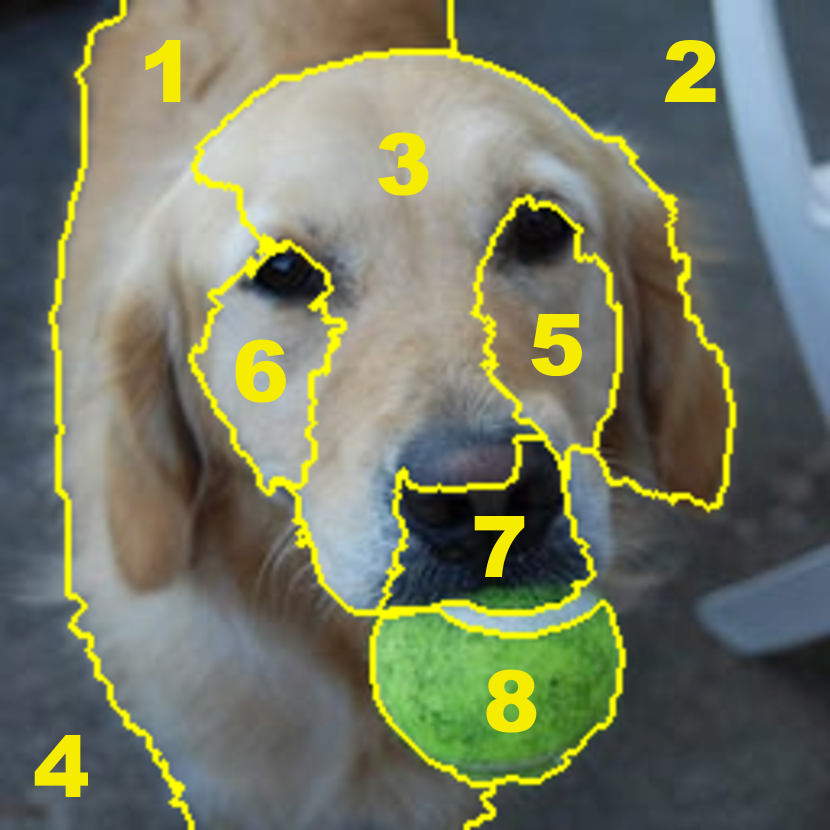
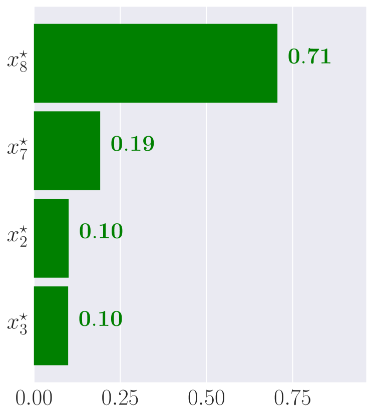
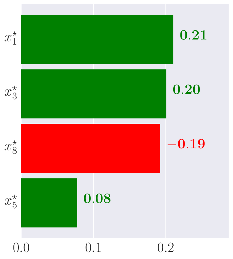
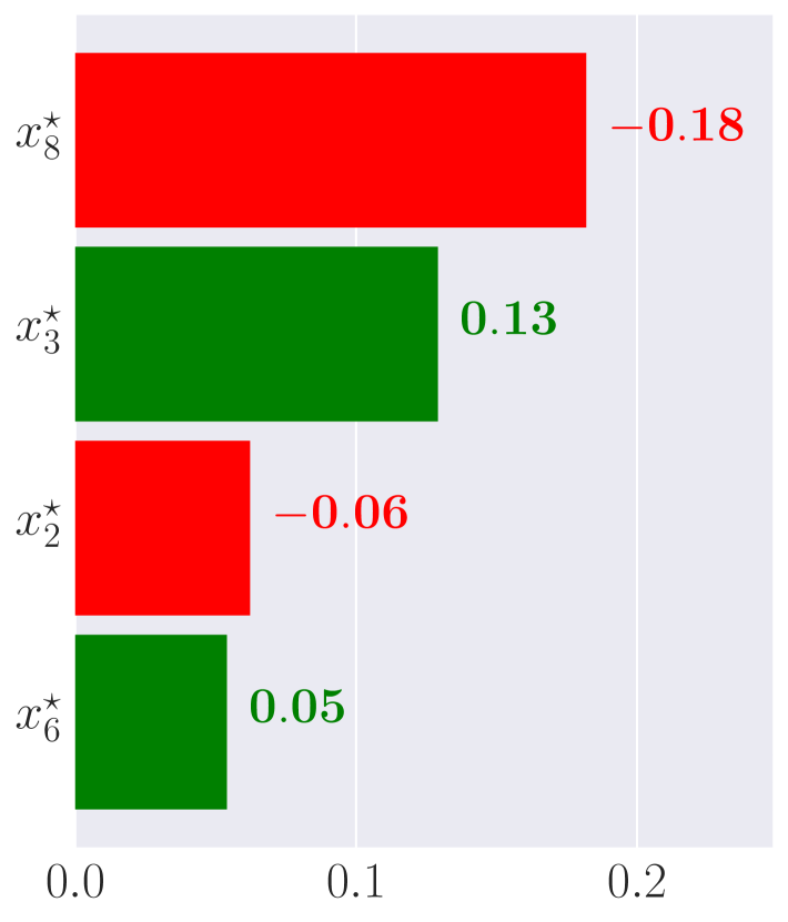
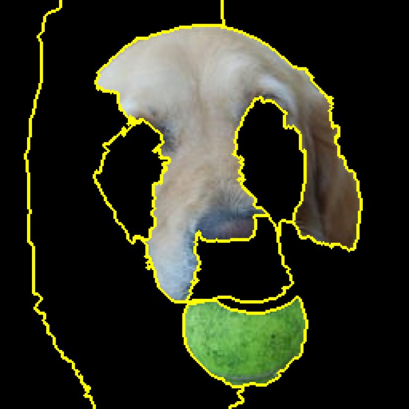
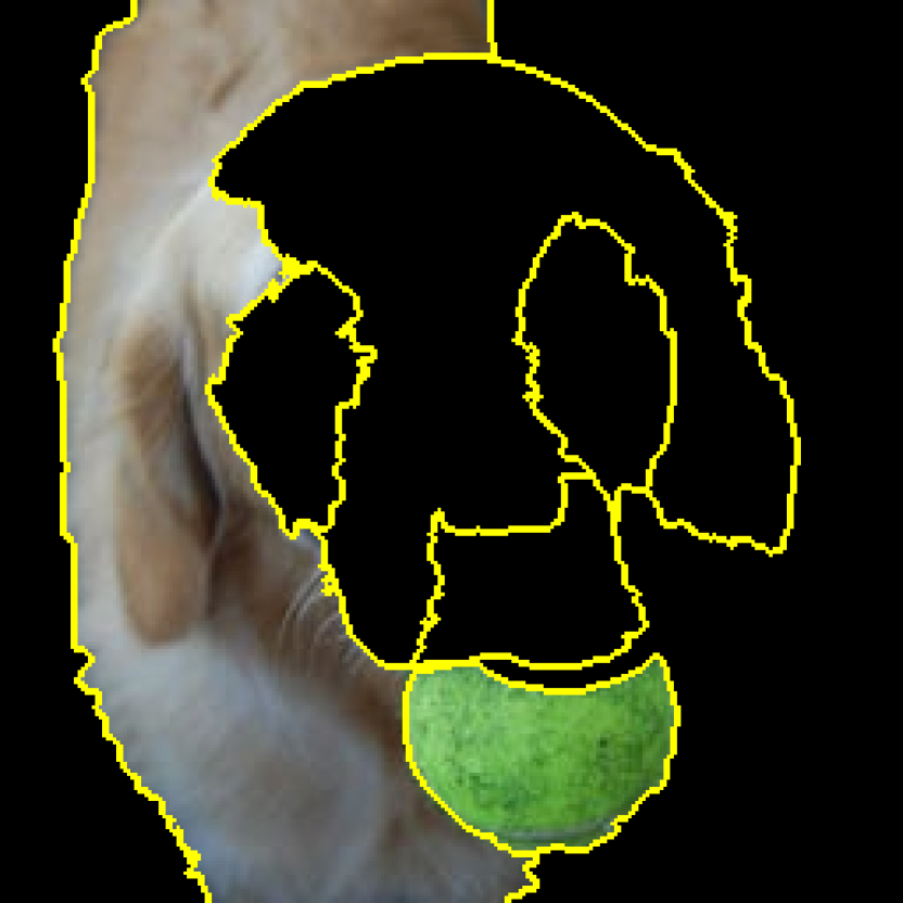
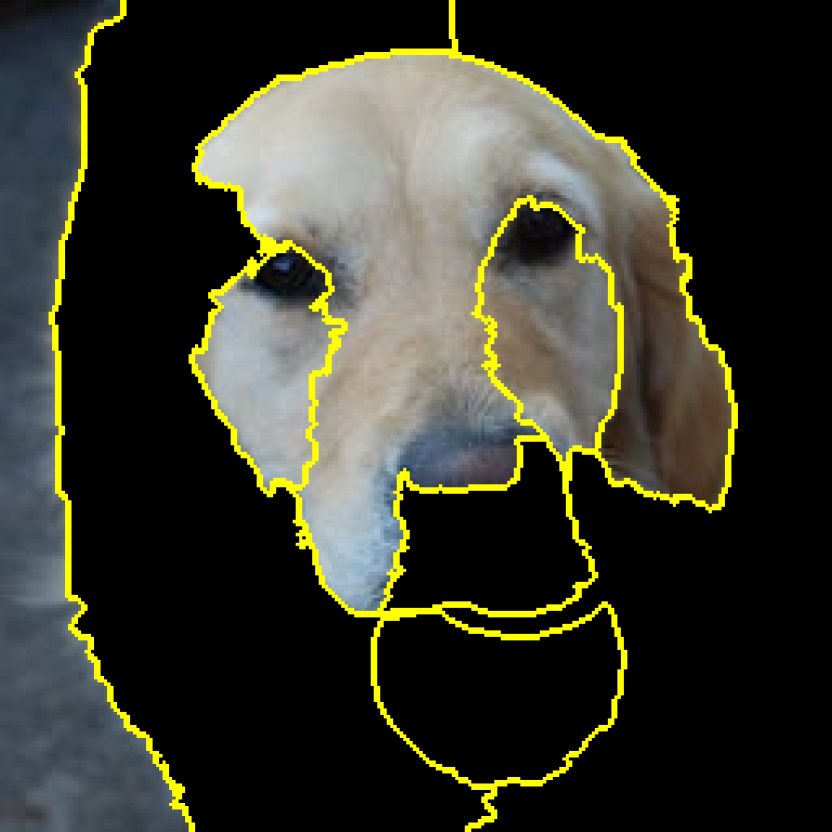
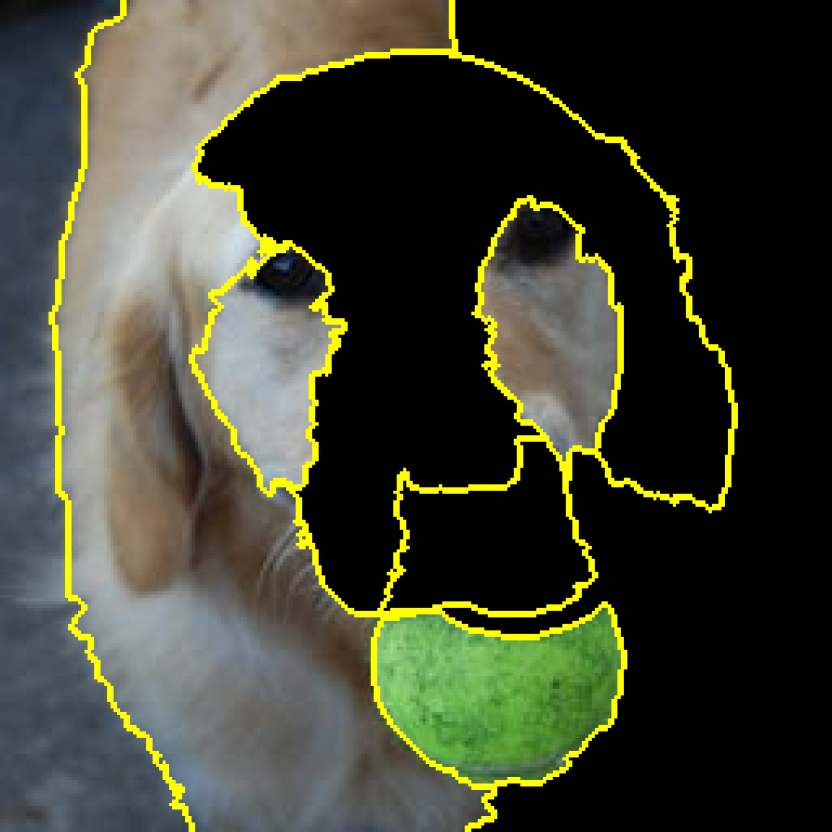
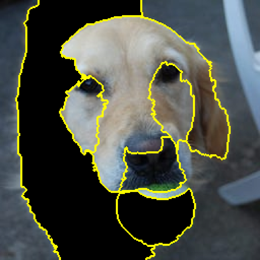
Figure 1 shows (1(a)) a segmentation-based interpretable representation of the image selected to be explained and (1(b), 1(c) & 1(d)) LIME explanations for the top three classes predicted for this data point by a black-box model. More details about the explanation process for image, text and tabular data domains can be found in the LIME paper (Ribeiro et al., 2016). Further analysis of surrogate explainers is offered by the bLIMEy framework (Sokol et al., 2019), which outlines a generic process for designing, building and testing bespoke surrogate explainers. An in-detail investigation of surrogate building blocks, their role, capabilities and limitations – concerning interpretable representations in particular – is also available (Sokol and Flach, 2020b). A more general discussion of surrogate explainers (Sokol, 2021) and their operationalisation (Sokol et al., 2022a) can be found as well. The following section summarises the most important limitations of surrogate linear models such as LIME.

2.2. LIME Trade-offs

The bLIMEy framework identifies three core components of surrogate explainers – interpretable representation, data sampling and explanation generation – which in this paper we consider in view of image data (Sokol et al., 2019). Specifically, LIME builds a sparse linear model as the surrogate used to generate explanations. In the image domain, instances are sampled in the interpretable representation – binary vectors encoding presence and absence of super-pixels – to ensure that the neighbourhood exploration offers meaningful data points. Since we are concern with explaining image predictions, we work with occlusion-based interpretable representations, whose properties and limitations are well studied (Sokol and Flach, 2020b).

Interpretable Representation Configuration

Choosing the granularity of segmentation and the operationalisation of the information removal proxy requires careful consideration. It is best to allow the explainee to tune the area and location of super-pixels, which allows for personalised and meaningful explanations (Sokol and Flach, 2020c); nonetheless, edge-based, algorithmic segmentation with a small number of regions can be useful whenever we need to automate this process (Sokol and Flach, 2020b). Selecting the occlusion colour – which acts as a reference point of the ensuing explanations (Mittelstadt et al., 2019) – is also crucial as it may bias the explanations; for example, using green for the image shown in Figure 1(a) is likely to prevent the surrogate from identifying the tennis ball super-pixel (#8) as an influential segment (Sokol and Flach, 2020b). LIME’s choice of occluding each partition with its mean colour (Ribeiro et al., 2016) is also subpar as it decreases the amount of information (by “blurring” the image) instead of removing it, thus making this proxy ineffective (Sokol and Flach, 2020b). This phenomenon is especially pronounced when working with a high number of segments, which results in them being smaller, hence their pixels being more colour-uniform – replacing such patches with their mean colour often yields patterns that preserve enough information for a predictive model to recognise the image class correctly.

Linear Model Assumptions

Using the family of linear models as surrogates propagates their assumptions and limitations onto the resulting explanations. Linear classifiers are unable to model target variables that are non-linear with respect to data features, a property that does not necessarily hold for high-level meta-features such as image segments. Correlations and interactions among data features may also have adverse effects on the quality of such explanations. The latter observation is particularly pertinent to interpretable domains whose features are highly inter-dependent, e.g., adjacent image segments. Given the nature of interpretable representations based on super-pixel segmentation and the intrinsic characteristics of linear models, addressing these shortcomings may be impossible without replacing either of these two components. Additionally, modelling probabilities of a class selected to be explained with a linear regression risks confusing the explainee who expects an output bounded between $0$ and $1$ but may be given a numerical prediction outside of this range.

Low Explanation Fidelity and Stability

The flexibility and generality of LIME – it is post-hoc and model-agnostic – also contribute to the instability and occasional unreliability of its explanations (Laugel et al., 2018; Zhang et al., 2019a; Sokol et al., 2019; Sokol and Flach, 2020b; Sokol et al., 2022a). If random sampling is employed, there are no guarantees with respect to reproducibility and stability of the explanations unless the random seed is fixed, which only provides an illusion of stability. A better approach may be to generate a full (binary) sample, which is often feasible given that interpretable representations of images tend to be small to ensure their human-comprehensibility (Sokol and Flach, 2020b). Good local fidelity of the surrogate model, i.e., its predictive coherence with respect to the underlying black box, is also not guaranteed and may be difficult to achieve. Notably, these problems are not limited to LIME or surrogate explainers but apply more broadly to post-hoc methods and are a major factor inhibiting their uptake (Rudin, 2019). High parameterisation and a wide array of possible component choices when building surrogates further contributes to their unreliability: number of samples, distance metric, kernel (width), interpretable representation (segmentation) and occlusion colour, to name a few (Garreau and von Luxburg, 2020; Sokol, 2021; Sokol et al., 2022a). Moreover, since surrogates only (locally) approximate the complex behaviour of a black-box model, such explanations may be misleading if their fidelity and limitations are miscommunicated to the explainee.

One Class Limitation

LIME explanations are confined to a single class – a separate linear regression needs to be fitted to (the probabilities of) each class of interest – which makes the process of discovering the dependencies between multiple classes challenging. For example, the same super-pixels may be influential – to different degrees – for two separate classes, leading to a potential confusion; a complete lack of overlap between influential segments may have the same effect. Since each explanation is derived from an independent linear model, the explanations need to be interpreted in isolation, forcing the user to relate them and draw conclusions that may lack theoretical grounding and validity.

3. Consistent Multi-class Explanations with LIMEtree

The major drawback of LIME and most other XAI and IML techniques is their limitation to explaining only one class at a time. Surrogates, for example, require us to fit a regression model to the probabilities predicted by the explained black box separately for each class, in which case the explainers produce implicit one-vs-rest insights. Beyond binary classification cases, a surrogate trained for class $A$ can only answer questions about the probability of this single class, with the complementary probability $p(\neg A)=1-p(A)$ modelling the union of all the other possible classes $\neg A=B\cup C\cup\dots$. Such explanations, e.g., counterfactuals, are thus limited to answering “Why $A$ rather than $\neg A$?” questions, which may have insufficient explanatory power for certain tasks. Interpreting the magnitude of the probability $p(A)$ output by a surrogate trained for class $A$ can also be problematic when explaining multi-class black boxes. If $p(A)$ is (much) greater than $0.5$, class $A$ is clearly dominant and by and large we do not need to worry about the remaining classes. If $p(A)\leq 0.5$, however, we cannot be certain whether there is a single class $B$ with $p(B)>p(A)$ or alternatively the combined probability of all the complementary classes $p(\neg A)$ is greater than or equal to $p(A)$ with no single class dominating over $p(A)$.

While per-class surrogate regressors prevent us from composing consistent multi-class explanations, this challenge can be overcome by employing surrogates that are multi-class classifiers. Using this model type allows us to explicitly answer both “Why $A$ rather than $\neg A$?” and “Why $A$ rather than $B$?” questions, thus uncover (coherent) relations between multiple classes albeit with some fundamental limitations. Such explanations are more powerful and natural to the explainee, but this approach confines us to black boxes that are crisp classifiers, or forces us to transform probabilities to class predictions when dealing with probabilistic models. The latter operation is sub-optimal as it results in a loss of important information about the confidence of the model’s predictions. For example, consider a situation in which the top two classes are almost equally likely – $p(A)=0.49$ and $p(B)=0.48$ – and a scenario where one of them is dominant – $p(A)=0.98$ – with both cases becoming indistinguishable. Additionally, deriving crisp predictions from probabilistic output prevents the explanations from simultaneously communicating the likelihood of all the classes. Addressing all of these challenges is important as most commonly used black-box predictive models in need of explainability deal with a large number of classes and are probabilistic, e.g., neural networks. This is especially true for image classification and object recognition tasks – e.g., the popular ImageNet data set (Deng et al., 2009) has 1,000 target labels – which we focus on in this paper.

3.1. LIMEtree: Surrogate Multi-output Regression Tree Explainer

We address the challenge of simultaneously explaining multiple classes of a prediction output by a probabilistic model by proposing a first-of-a-kind surrogate explainer based on a multi-output regression tree, which provides the best of both worlds. It simulates multi-class modelling in a regression setting, allowing the surrogate to capture interactions between multiple classes, hence explain them coherently – see the example shown in Figure 2. This is a significant improvement over training a separate one-vs-rest regression surrogate for each explained class, which may produce diverse, inconsistent, competing or contradictory explanations – thus risk confusing the explainees and put their trust at stake – whenever these models do not share a common tree structure or split on different feature subsets. Since class probabilities predicted by the black box and used as target variables for training the surrogate are highly correlated, independent one-vs-rest surrogates cannot easily capture their intricate dependencies. For example, an increase in the predicted probability of class $A$ causes the probability of another class $B$ to decrease, which plays an important role among the top classes predicted by a black box. Multi-output regression surrogates can model these relationships faithfully and transparently as each of their nodes displays the estimated probabilities of every explained class, thus reflecting how individual interventions in the interpretable domain affect these values. Our contributions establish a new direction in XAI and IML research – concerned with consistent and faithful explanations of multiple classes – and offer a first method to address this challenge.

Figure 2. Surrogate multi-output regression tree explaining the top three classes – tennis ball, golden retriever and Labrador retriever – predicted by a black-box model for the image shown in Figure 1(a). The segments shaded in blue do not influence the explanation at a given tree node, i.e., they can either be preserved or discarded for the explanation to hold. A super-pixel whose value is $0$ in the interpretable representation is “removed” by occluding it with a solid black colour. A super-pixel assigned $1$ in the interpretable representation is preserved. The class probabilities estimated by each node of the surrogate tree may not sum up to $1$ as these values capture a subset of the modelled classes and are a result of numerical regression, hence should not be treated as probabilities per se.

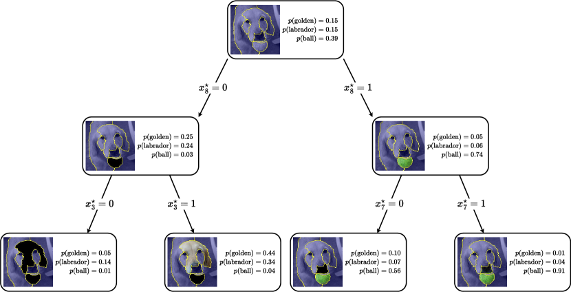
Using Classification And Regression Trees (CART (Breiman et al., 1984)) as our surrogates additionally allows us to address the shortcomings identified when linear models are used to this end (Sokol et al., 2019; Sokol and Flach, 2020b; Sokol, 2021) – refer to Section 2.2. Trees neither presuppose independence of (the interpretable) features nor existence of a linear relationship between (the interpretable) features and the target variable. The availability of a broad range of diverse explanation types – examples of which are provided in Section 4.1 – makes this family of models a particularly good candidate for surrogates (Sokol, 2021). Using them also allows us to achieve near full or full explanation fidelity – see Section 3.2 – which further adds to their appeal. While surrogate regression trees that approximate the probability of a single class are guaranteed to output a number within the $[0,1]$ range – the estimate is calculated as the mean value, which lies between the minimum and the maximum, of the training data targets assigned to a given tree node – this may not necessarily hold for multi-output trees. Approximating probabilities of multiple classes by averaging their values across a number of instances may yield estimates whose sum is greater than $1$, nonetheless these values can be easily rescaled to avoid confusing the explainees.

To ensure low complexity and high fidelity of our multi-output regression trees, we employ the same optimisation objective $\mathcal{O}$ as given in Equation 1. Since we are using surrogate trees, we modify the model complexity function $\Omega$ to measure either the depth of the tree or its width (number of leaves) as given by Equation 4, where $d$ is the dimensionality of the binary interpretable domain $\mathcal{X}^{\star}$. The choice between the two mostly depends on the type of the explanation that we want to extract from the surrogate tree; for example, depth may be preferred when visualising the tree structure or extracting decision rules. In certain cases, such as unbalanced trees with the extreme case being a one-sided tree, optimising for width or a combination of the two may be more desirable. We also adapt the loss function $\mathcal{L}$ to account for the surrogate tree $g$ outputting multiple values in a single prediction as shown in Equation 5, where $\mathring{C}$ are the classes to be explained by $g$, for which the $c$ subscript in $g_{c}(x^{\star})$ indicates prediction of a selected class $c\in\mathring{C}$ for the data point $x^{\star}$.

(4) $$\Omega(g;\;d)=\frac{\text{depth}(g)}{d}\;\;\;\;\text{or}\;\;\;\;\Omega(g;\;d)=\frac{\text{width}(g)}{2^{d}}$$

(5) $$\mathcal{L}(f,g;\;\mathcal{X}^{\star},\mathring{x},\mathring{C})=\frac{1}{\sum_{x^{\star}\in\mathcal{X}^{\star}}\omega(x^{\star};\;\mathring{x})}\;\sum_{x^{\star}\in\mathcal{X}^{\star}}\left(\omega(x^{\star};\;\mathring{x})\;\frac{1}{1+\mathbbm{1}(|\mathring{C}|>1)}\;\sum_{c\in\mathring{C}}\left(f_{c}\left(\mathit{IR}^{-1}(x^{\star})\right)-g_{c}(x^{\star})\right)^{2}\right)$$

Note that the inner sum over the explained classes $\sum_{c\in\mathring{C}}$ is normalised by $\frac{1}{1+\mathbbm{1}(|\mathring{C}|>1)}$, which becomes $1$ when the surrogate is built for a single class (i.e., $|\mathring{C}|=1$) and is $\frac{1}{2}$ for more classes (i.e., $|\mathring{C}|>1$). Therefore, the loss function given by Equation 5 is equivalent to the one given by Equation 3 in the former case, and in the latter the scaling factor ensures that the inner sum is between $0$ and $1$ since the biggest squared difference is $2$ – this happens when the predictions of $f$ and $g$ assign a probability of $1$ to two different classes, e.g., $[1,0,0]$ and $[0,0,1]$. An additional assumption is that the sum of values predicted by each leaf of the surrogate tree is smaller or equal to $1$, which as noted earlier may in some cases require normalisation. The outer sum $\sum_{x^{\star}\in\mathcal{X}^{\star}}$ is scaled by the sum of weights $\omega(x^{\star};\;\mathring{x})$ to ensure that the loss $\mathcal{L}$ is bounded between $0$ and $1$, facilitating a direct comparison of different surrogates and allowing for a meaningful user-defined stopping criterion when implementing this paradigm. In practice, this surrogate explainer is built by (re)training a multi-output regression tree while iteratively increasing the depth or width bound imposed upon it – thus rising its complexity $\Omega(g;\;d)$ but also improving its predictive power – which allows to further minimise the loss $\mathcal{L}$ and optimise the objective function $\mathcal{O}$. This procedure terminates when the loss $\mathcal{L}$ defined by Equation 5 reaches a certain, user-defined level $\epsilon\in[0,1]$, which corresponds to the fidelity of the local surrogate, i.e., $\mathcal{L}\left(f,g;\;\mathcal{X}^{\star},\mathring{x},\mathring{C}\right)\leq\epsilon$.

Data: $\bullet$ explained data point $\mathring{x}$ $\bullet$ set of classes to be explained $\mathring{C}\subseteq\mathcal{C}$ $\bullet$ black-box model $f$ $\bullet$ interpretable representation transformation function $\mathit{IR}$ and its inverse $\mathit{IR}^{-1}$ $\bullet$ samples number $n$ $\bullet$ distance function $L$ $\bullet$ kernel $k$ $\bullet$ tree depth bound $d$ $\bullet$ fidelity expected of the local surrogate $\epsilon$

Result: local surrogate multi-output regression tree

1 Build interpretable representation of the explained instance $\mathit{IR}(\mathring{x})=\mathring{x}^{\star}$;

2 $X^{\star}\leftarrow$ sample $n$ data points from the interpretable domain $\mathcal{X}^{\star}$ or generate a full sample;

3 Transform the sample into the original domain $\mathcal{X}$ with $\mathit{IR}^{-1}(X^{\star})=X$;

4 Predict the probabilities of $X$ with the black-box model $f$;

5Compute the distance between $\mathring{x}^{\star}$ and the sample $X^{\star}$ using $L$;

6Compute the weights by kernelising the distance with $k$;

7 for $i\in[1,\ldots,d]$ do

8       Fit a multi-output regression tree $g$ with a depth bound $i$ to the weighted data sample $X^{\star}$ using the specified subset $\mathring{C}$ of class probabilities predicted by the black box in step 1 as the target;

9      Evaluate the fidelity $\mathcal{L}$ of the surrogate;

10       Break the loop when the surrogate achieves the user-defined fidelity $\epsilon$, i.e., $\mathcal{L}\leq\epsilon$;

11 end for

12 Return the optimal multi-output regression tree surrogate;

Algorithm 1 LIMEtree.

Putting everything together leads to Algorithm 1, which we call LIMEtree. While it is relatively lightweight, manipulating images via the $\mathit{IR}$ and $\mathit{IR}^{-1}$ functions and querying the black-box model $f$ may become a bottleneck. The explainee has no control over the computational and memory complexity of querying the black box, which is executed $n$ times, where $n$ is the number of sampled data points. Given the recent advances in dedicated machine learning hardware, this step should not be a burden when utilising GPUs and manageable with just CPUs. Transforming the interpretable representation (binary vectors) into the original domain (images) requires a considerable amount of operational memory – the explained image has to be duplicated for every data point sampled from the interpretable domain and its pixel values need to be altered to reflect segment occlusions. The efficiency of these two steps can be significantly improved with batch processing and parallelisation, therefore reducing the use of memory and improving the processing time. Other steps in Algorithm 1 are relatively efficient: segmenting the explained image, sampling a binary matrix from the interpretable domain and fitting a multi-output regression tree to binary data with feature thresholds fixed at $0.5$.

3.2. LIMEtree Fidelity

Our multi-output regression trees can significantly improve the local fidelity of explanations, thus address a major criticism of surrogate explainers (Rudin, 2019). To this end, we identify the minimal interpretable representation $X^{\star}_{T}$, which is a set of instances unique to each tree, in Definition 3.1. It is composed of binary vectors $x^{\star}_{t}$ drawn from the interpretable representation $\mathcal{X}^{\star}$ – one for each leaf $t\in T$ of the surrogate decision tree – that have the least number of $0$ components while still being assigned to the leaf $t$. This can be understood as looking for the minimal possible occlusion of an image for each leaf of the tree since a $0$ component of a vector in the interpretable representation indicates segment occlusion.

Definition 3.1.

Assume a binary decision tree $g\in\mathcal{G}$ fitted to a binary $d$-dimensional data space $\mathcal{X}^{\star}=\{0,1\}^{d}$, with $T$ denoting its set of leaves. This tree assigns a leaf $t\in T$ to a data point $x^{\star}\in\mathcal{X}^{\star}$ with function $g_{\mathit{id}}(x^{\star})=t$. For a selected tree leaf $t$, the unique minimal data point $x^{\star}_{t}$ is given by:

$$x^{\star}_{t}=\operatorname*{arg\,max}_{x^{\star}\in\mathcal{X}^{\star}}\sum_{i=1}^{d}x^{\star}_{i}\;\;\;\;\text{s.t.}\;\;\;\;g_{\mathit{id}}(x^{\star})=t\text{,}$$

where $x^{\star}_{i}$ is the $i$^th component of the binary vector $x^{\star}$. We can further define a minimal set of data points $X^{\star}_{T}\subseteq\mathcal{X}^{\star}$, uniquely representing a tree $g$ and the set of its leaves $T$, which is composed of all the minimal data points for this tree:

$$X^{\star}_{T}=\{x^{\star}_{t}:t\in T\}\text{.}$$

Next, we transform this minimal representation set $X^{\star}_{T}$ from the interpretable into the original domain $\mathcal{X}$, i.e., images, using the inverse of the interpretable representation transformation function $X_{T}=\{\mathit{IR}^{-1}\left(x^{\star}_{t}\right):x^{\star}_{t}\in X^{\star}_{T}\}$. We then predict class probabilities for each image in $X_{T}$ with the black box $f$ and replace the values estimated by the surrogate tree with these probabilities for each leaf $t\in T$, i.e., modify the surrogate tree by overwriting its predictions. Doing so is only feasible for the tree leaves as the minimal data points for some of the splitting nodes are indistinguishable; for example, all of the nodes on the root-to-leaf path that decides every interpretable feature to be $1$ are non-unique and all would be represented by the original (non-occluded) image. This procedure – called LIMEtree and summarised by Algorithm 2 – ensures full local fidelity of the surrogate tree with respect to the explanations derived from the tree structure such as counterfactuals and root-to-leaf decision rules (see Section 4.1 for their examples). However, for this property to hold the function transforming data from the original domain into the interpretable representation $\mathit{IR}$ has to be deterministic (Sokol and Flach, 2020b) as outlined in Lemma 3.2, which follows from the discussion presented in the next paragraph.

Data: $\bullet$ black-box model $f$ $\bullet$ local surrogate multi-output regression tree $g$ $\bullet$ interpretable representation transformation function $\mathit{IR}$ and its inverse $\mathit{IR}^{-1}$ $\bullet$ set of classes to be explained $\mathring{C}\subseteq\mathcal{C}$

Result: surrogate multi-output regression tree with full local fidelity

1 $T\leftarrow$ identify the set of leaves of the surrogate model $g$;

2 $X_{T}^{\star}\leftarrow$ compose the set of data points constituting the minimal interpretable representation (see Definition 3.1);

3Transform this set into the original domain $\mathcal{X}$ with $\mathit{IR}^{-1}(X_{T}^{\star})=X_{T}$;

4 Predict the probabilities of $X_{T}$ with the black-box model $f$;

5for $t\in T$ do

6       Replace the probabilities predicted by the leaf $t$ of the surrogate $g$ with the black-box predictions (step 2) of this leaf’s minimal data point $x^{\star}_{t}\in X_{T}^{\star}$ (step 2) for the specified subset of classes $\mathring{C}$;

7 end for

8Return the multi-output surrogate regression tree $g$ with full local fidelity;

Algorithm 2 LIMEtree.

Lemma 3.2.

A decision tree surrogate can achieve full fidelity with respect to the explanations derived from the structure of this tree – model-driven explanations – if the function $\mathit{IR}:\mathcal{X}\mapsto\mathcal{X}^{\star}$ transforming data from their original domain $\mathcal{X}$ into an interpretable representation $\mathcal{X}^{\star}$ is deterministic. This means that $\mathit{IR}$ is a one-to-one mapping from $\mathcal{X}$ to $\mathcal{X}^{\star}$, with the corresponding unique inverse function defined as $\mathit{IR}^{-1}:\mathcal{X}^{\star}\mapsto\mathcal{X}$. Therefore, a data point $x\in\mathcal{X}$ can be translated into a unique data point $\mathit{IR}(x)=x^{\star}\in\mathcal{X}^{\star}$ and vice versa $\mathit{IR}^{-1}(x^{\star})=x$.

Lemma 3.2 guarantees that each leaf in the surrogate tree is associated with only one data point $x_{t}$ in the original representation $\mathcal{X}$. This instance is derived from the minimal interpretable data point $x^{\star}_{t}$ by applying the inverse of the interpretable representation transformation function $\mathit{IR}^{-1}$, i.e., $x_{t}=\mathit{IR}^{-1}(x^{\star}_{t})$. Therefore, $x_{t}$ represents the original image with the smallest possible number of occluded segments such that $g_{\mathit{id}}(x^{\star}_{t})=t$. By assigning the probabilities predicted by the explained black box for each data point $x_{t}$ to the corresponding leaf $t$ of the surrogate, it achieves full fidelity for the minimal representation set $X_{T}$, which is the backbone of model-driven explanations. The interpretable representation for images used in this paper and by LIME (Ribeiro et al., 2016) – super-pixel segmentation with solid colour occlusion as the information removal proxy – is deterministic since the segmentation and occlusion strategy are fixed (Sokol and Flach, 2020b).

While the procedure outlined in Algorithm 2 ensures full fidelity of model-driven explanations, the same is not guaranteed for data-driven explanations such as answers to what-if questions, e.g., “What if segments #3, #5 and #7 were absent?” Root-to-leaf paths that do not condition on all of the binary interpretable features allow for more than one data point to be assigned to that leaf, e.g., for three binary features $(x^{\star}_{1},x^{\star}_{2},x^{\star}_{3})\in\{0,1\}^{3}$, a root-to-leaf path with a $x^{\star}_{1}<0.5\land x^{\star}_{3}<0.5$ condition assigns $(0,0,0)$ and $(0,1,0)$ to this leaf. This observation prompted us to specify the minimal interpretable representation $X^{\star}_{T}$ (Definition 3.1) that selects a single data point to represent each leaf, thereby facilitating full fidelity of model-driven explanations without additional assumptions. However, to achieve full fidelity for data-driven explanations, the surrogate tree must faithfully model the entire interpretable feature space, i.e., have one leaf for every data point in this feature space, which can be thought of as extreme overfitting. Since the cardinality of a binary $d$-dimensional space $\mathbb{B}^{d}=\{0,1\}^{d}$ is equal to $|\mathbb{B}^{d}|=2^{d}$, and a complete and balanced binary decision tree of $2^{d}$ width (number of leaves) is $d$ deep, relaxing the tree complexity bound $\Omega$ accordingly guarantees full fidelity of all the explanations, which is expressed in Corollary 3.3.

Corollary 3.3.

If the complexity bound $\Omega$ (width) of a surrogate tree $g$ is relaxed to equal the cardinality of the binary interpretable domain $\mathcal{X}^{\star}$, i.e., $\Omega(g;\;|\mathcal{X}^{\star}|)=\frac{\text{width}(g)}{2^{|\mathcal{X}^{\star}|}}=\frac{2^{|\mathcal{X}^{\star}|}}{2^{|\mathcal{X}^{\star}|}}=1$, then the surrogate is guaranteed to achieve full fidelity. This property applies to explanations that are both:

data-driven:

derived from any data point in the interpretable representation, and

model-driven:

derived from the structure of the surrogate tree.

Therefore, a surrogate tree that guarantees faithfulness of model-driven explanations (Lemma 3.2 and Algorithm 2) can only deliver trustworthy counterfactuals and exemplar explanations sourced from the minimal representation set. For such surrogates we can also generate what-if explanations with full fidelity by bypassing the surrogate tree and directly querying the black-box model. This may be an attractive alternative to more complex surrogate trees that additionally guarantee faithfulness of data-driven explanations (Corollary 3.3) whenever the black-box predictive function is accessible and querying it is not prohibitively expensive (in time or compute). The latter surrogate type, which usually yields deeper trees, can deliver a broader spectrum of trustworthy explanations: tree structure-based explanations, feature importance, decision rules (root-to-leaf paths), answers to what-if questions and exemplar explanations based on any data point, in addition to counterfactuals.

4. Discussion: Examples, Analysis, Benefits and Guarantees

LIMEtree is highly flexible, supports different types of explanations and comes with strong fidelity guarantees. By tailoring the interpretable representation to a particular data set or data point – either statically or through user interaction – the explanations can be further personalised (Sokol and Flach, 2020b, c; Sokol, 2021). Additional customisation can be afforded by allowing the explainee to (dynamically) tweak the content of explanations (Sokol and Flach, 2020c). Notably, LIMEtree works equally well for data types other than image, e.g., tabular and text, and its full fidelity desideratum can be achieved in practice while maintaining low complexity of explanations. All of our design choices empower the users to build an explainer that best fits a particular use case (Sokol et al., 2022a), targeting a wide range of stakeholders and purposes, for example, model debugging, robustness analysis, fairness evaluation and explainability.

4.1. Diverse Explanation Types

While surrogate explainers based on linear models (such as LIME (Ribeiro et al., 2016)) are limited to producing insights based on influence of interpretable features – image segments in our case – employing trees offers us a selection of diverse explanation types. Specifically, we can generate high-fidelity artefacts such as:

1. visualisation of the tree structure;

2. tree-based (interpretable) feature importance;

3. logical conditions extracted from root-to-leaf paths;

4. exemplar explanations taken from training data falling into the same leaf;

5. answers to what-if questions generated based on the tree structure (i.e., by querying the tree); and

6. counterfactuals retrieved by comparing and applying logical reasoning to different tree paths.

The first two explanation types uncover the behaviour of a black box in a given data sub-space; the remainder targets specific predictions. Since all six explanation types are derived from a single (surrogate) model, they are guaranteed to be coherent and their diverse nature should appeal to a wide range of audience. While some of these explanations are inherently static, others can be embedded in an interactive explanatory dialogue, enabling the explainee to customise and personalise them in a natural way as we will explore in the following section. To better communicate LIMEtree’s explanatory power, we provide multiple examples of these explanation types for the top three classes predicted by a black box for the image shown in Figure 1(a) – tennis ball (99.28%), golden retriever (0.67%) and Labrador retriever (0.04%) – and compare them to the corresponding LIME explanations shown in Figure 1.

The LIME explanation for tennis ball – shown in Figure 1(b) – indicates that segment #8, which depicts the ball, has an overwhelmingly positive influence on predicting this class. Figure 1(b) also exemplifies the problem with high correlation of adjacent super-pixels: the next two most important segments are #2 and #7 – they are neighbours of #8 and mostly surround it – which is likely because they include pixels that belong to the tennis ball object, e.g., the characteristic white stripe (#2). The other two LIME explanations are for golden retriever (Figure 1(d)) and Labrador retriever (Figure 1(c)). In both cases the segment depicting the ball (#8) has a large negative influence, which is expected, and the segment capturing the dog’s face (#3) has a large positive effect. Predicting between these two dog breeds is determined by the positive effect of segment #1 on the golden retriever class (maybe because it reveals the long coat) and the negative influence of segment #2 on the Labrador retriever class (possibly since it includes the white stripe of the tennis ball). Based on this evidence alone, it is difficult to determine the model’s heuristic for telling apart these two classes; in particular, the role that segment #2 plays.

(a) Tree-based feature importance – all three classes share one explanation.

(b) What-if explanation: “What if the ball was not there?” $\rightarrow$ 97% golden retriever.

(c) Exemplar explanation: “Show me an example of a golden retriever.”

(d) Exemplar explanation: “Show me an example of a Labrador retriever.”

Figure 3. Three types of LIMEtree explanations: (3(a)) feature importance, (3(b)) what-if explanation and (3(c) & 3(d)) exemplar explanations.

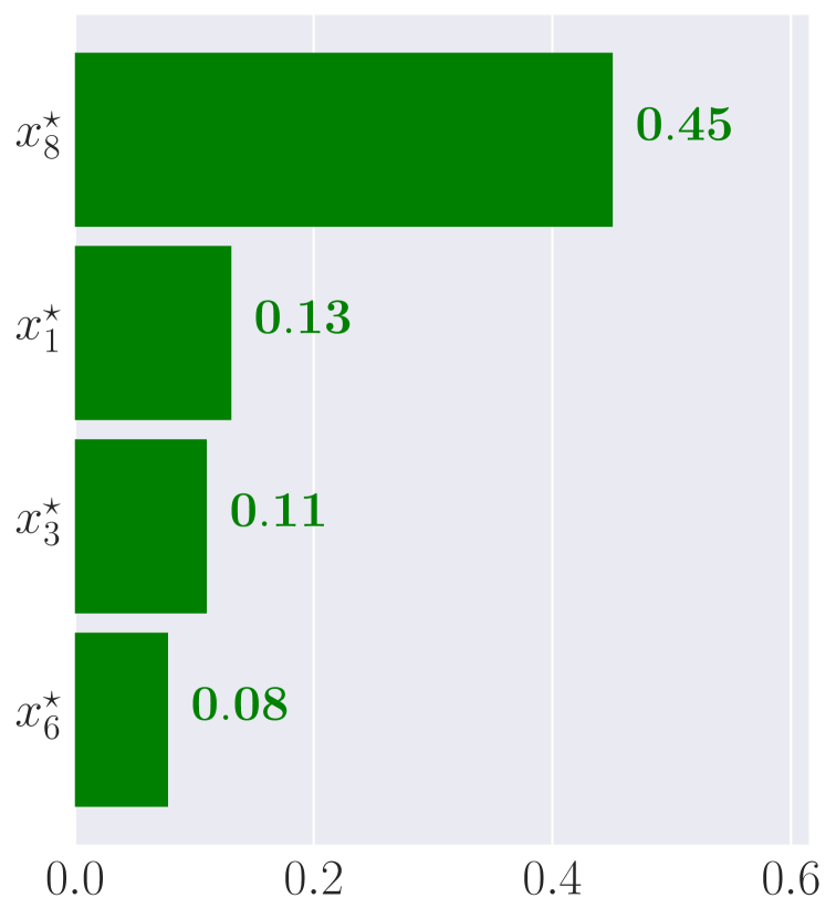
When it comes to LIMEtree, we can easily calculate the importance of interpretable features (Gini importance (Breiman, 2001)) – shown in Figure 3(a) – which closely resembles LIME insights. Since LIMEtree models all three classes simultaneously, the importance captures the segments that help to differentiate between these classes. Comparing Figure 3(a) with analogous LIME explanations shown in Figure 1 reveals a reassuring overlap, with each LIME explanation sharing at least two of its top four most important segments with the LIMEtree explanation. The tree-based feature importance indicates that segment #8 – depicting the ball – is the most important, owing to the dominant tennis ball prediction (99.28%), and is followed by segments #1, #3 and #6 – covering most of the dog. While informative, these insights cannot be explicitly attributed to any individual class and the feature importance values can only be positive, limiting their explanatory power.

Since all LIMEtree explanations are consistent – they are derived from the same surrogate tree – with some help of another explanation type, such as the tree structure visualisation shown earlier in Figure 2, we can discover the relation between each important feature (Figure 3(a)) and the three explained classes. It is important to note that these two explanations are derived from different trees since the depth of the surrogate shown in Figure 2 was limited to 2 for visualisation purposes; this also means that we can achieve full fidelity with respect to model-driven explanations (Lemma 3.2) but not data-driven explanations (Corollary 3.3). Comparing the two leftmost leaves with the two rightmost ones – the result of the root split on segment #8 – tells us that this segment has positive influence on the tennis ball prediction; additionally, when segment #7 is present this prediction is strengthened, nonetheless without it tennis ball is still the most likely prediction. On the other hand, when the ball is absent, i.e., segment #8 is occluded, both dog breeds are almost equally likely with the presence of segment #3 being the deciding factor: it is Labrador retriever if #3 is occluded and golden retriever if #3 is present (although Labrador retriever is nearly equally likely in this case).

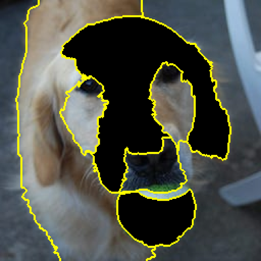
Arriving at these conclusions required us to inspect and reason over the tree structure, which cannot be expected of a lay explainee or when the surrogate tree is large or complex. In such cases we can use other types of explanations, for example, what-if questions. Since the tree presented in Figure 2 is not complete (see Lemma 3.2), we use the black-box model instead of the surrogate to evaluate the hypothetical scenarios. Because segment #8, depicting the ball, is the most important factor, we are interested in what if this segment was not there; the new prediction is 97% golden retriever – see Figure 3(b). We can also ask for exemplar explanations of the golden retriever and Labrador retriever classes, which are shown in Figures 3(c) and 3(d) respectively.

In order to take full advantage of LIMEtree explanations, we train a complete surrogate tree (see Corollary 3.3). We use it to retrieve the shortest possible explanation, i.e., with the highest number of occluded segments, of tennis ball. There are three such explanations of length two – shown in Figure 5 – with the following pairs of super-pixels preserved: #7 & #8, #3 & #8 and #1 & #8. We can also generate rule explanations of Labrador retriever based on the root-to-leaf paths found in the tree, selecting the one with the highest probability of this class. The resulting explanation is $x^{\star}_{1}=0\land x^{\star}_{2}=0\land x^{\star}_{3}=1\land x^{\star}_{4}=1\land x^{\star}_{5}=1\land x^{\star}_{6}=1\land x^{\star}_{7}=0\land x^{\star}_{8}=0$, yielding 98% confidence. Such a representation is not particularly appealing, especially to a lay audience, but we can improve its comprehensibility by transforming it to the visual domain – see Figure 5.

(a) Segments #8 and #7 preserved $\rightarrow$ 97% tennis ball.

(b) Segments #8 and #3 preserved $\rightarrow$ 92% tennis ball.

(c) Segments #8 and #1 preserved $\rightarrow$ 51% tennis ball.

Figure 4. The shortest (highest number of occlusions) LIMEtree explanations of tennis ball.

Figure 5. Visual representation of a LIMEtree rule explanation that maximises the probability of Labrador retriever (98%).

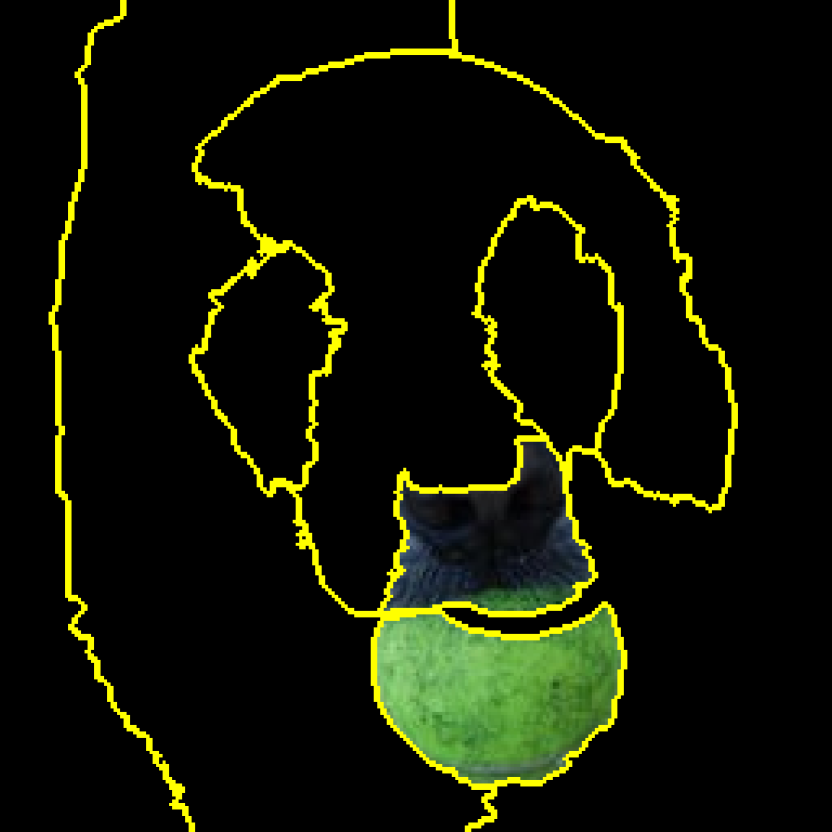
The biggest advantage of LIMEtree is its ability to output counterfactual explanations by using any method compatible with (regression) trees (Sokol, 2021). For example, we can ask the following question: “Given segment #8 (the ball), what would have to change for the image to be classified as golden retriever?” Therefore, we are looking for an image occlusion pattern that preserves the ball segment (#8) and yields golden retriever prediction. LIMEtree tells us that by discarding super-pixels #2, #3 and #7 – the smallest viable occlusion shown in Figure 6(a) – the model predicts golden retriever (54%). Since occluding segment #8, i.e., the ball, results in 97% golden retriever (see Figure 3(b)), another interesting question is: “Had segment #8 not been there, can the model still predict tennis ball?” LIMEtree indicates that this can be achieved by occluding segments #1 and #8 as shown in Figure 6(b).

(a) How we can get a golden retriever prediction (54%) given #8.

(b) Occluding segments #8 and #1 yields tennis ball (94%) according to the black box.

Figure 6. Customised counterfactual explanations generated by LIMEtree.

4.2. Personalised and Interactive Explainability

No matter how comprehensive an explanation is, it may not appeal to all explainees or answer all their questions (Sokol and Flach, 2020c, 2018). Humans are accustomed to an explanatory process that entails interactive questioning, arguing and rebutting, which arises naturally in a conversation; therefore, for explanations of predictive systems to be intuitive, they should imitate this process (Miller, 2018). While linear surrogates such as LIME are confined to static, one-off and one-size-fits-all insights, certain explanations produced by tree-based surrogates can be framed in an interactive explanatory process, giving explainees the control over their composition (Sokol and Flach, 2018, 2020c). By extension, LIMEtree supports dynamic personalisation of various aspects of its explanations, in particular the interpretable representation as well as the explanation type and its content. This approach enables the explainees to steer the explanatory process in a selected direction, thereby achieving an explanation that satisfies their curiosity or answers a specific question.

Interpretable Representation

The first step towards personalised surrogate explanations is tuning the interpretable data representation (Sokol and Flach, 2020b; Sokol et al., 2019). While, in case of images, computer generated segments may be good enough to produce meaningful explanations, supporting the explainee in either providing custom segmentation or personalising computer-generated super-pixels can yield even better results (Sokol and Flach, 2020c). This step aims to achieve an interpretable representation that conveys meaningful concepts, which may be different for individuals with distinct levels of domain expertise and background knowledge. For example, the segmentation used throughout the example explanations provided in this paper (see Figure 1(a)) is a result of merging user-specified collections of super-pixels produced with an edge-based segmentation algorithm. Similar reasoning applies to tabular and text data where the explainee can respectively customise binning of continuous features and tokenisation of sentences, e.g., match together selected words to form a tuple considered as a single token in the interpretable representation (Sokol and Flach, 2020b). Since personalised interpretable representations tend to be small in size (see Figure 1(a)), fitting a complete tree (as per Corollary 3.3) is often easily achievable, providing access to a diverse range of faithful and comprehensible explanations.

Explanation Content

As noted earlier, counterfactual explanations play an important role in XAI and IML. They are often simple “Why?” questions with either implicit or explicit class contrast, e.g., “Why is it a cat?” where the implicit contrast is interpreted as “Why is it a cat and not anything else?”, or “Why is it a cat and not a lion?” where the explainee provides the contrast explicitly. Nonetheless, the user can also ask more elaborate “Why given?” and “Why despite?” questions to additionally take control of and personalise the (interpretable) features appearing in the conditional part of the explanation (Sokol and Flach, 2018, 2020c). An explainee may prefer a counterfactual that, respectively, must and/or must not be conditioned on certain attributes, e.g., “Why is it a golden retriever and not a Labrador retriever, given occluded segment #3 and despite visible segments #1 and #6?”, which specifies both these conditions and uses an explicit class contrast. Counterfactual explanations are capable of supporting such customisation via an interactive explanatory dialogue (Sokol and Flach, 2018, 2020c) and a compatible process of their retrieval can be implemented efficiently for decision trees (Sokol, 2021). This opportunity for personalisation is by extension available with LIMEtree, which uses multi-output regression trees as its underlying surrogate model, and the examples of counterfactual explanations presented in Section 4.1 rely on this procedure.

Answers to what-if questions are another explanation type available for surrogate trees that can be personalised through interaction. The explainee can formulate conditions on the interpretable features of a data point, say pertaining to image segments, and ask for its prediction, e.g., “What if segments #1 and #5 were occluded?” Such questions can be answered using either the black-box or the surrogate model depending on the accessibility and computational efficiency of the former as well as completeness and fidelity of the latter. Their personalisation power can be seen in the examples shown in Section 4.1, which rely on this property.

Interface and Presentation Medium

Another, weaker, form of interaction can be had with decision rules, i.e., root-to-leaf paths, and exemplars, i.e., similar data points. The first type allows the explainees to inspect the influence of each logical condition from this path on the prediction. In the image domain, for example, each root-to-leaf path could be visualised as the original image with a subset of segments occluded, with an interactive interface allowing the explainee to click on each super-pixel to switch its occlusion on or off, thereby changing the tree path, to understand its influence on the prediction. Similar interactive approaches can be developed for tabular and text data by allowing the explainee to change feature values and add or remove word-based tokens. Since exemplars are generated by identifying all the data points (in the interpretable representation) that fall into the same and similar (however this is defined) leaves of the surrogate tree, the interactivity of these explanations can rely on the aforementioned principle. The explainee could select a leaf for which to generate exemplars and specify whether these should be data points that are assigned the same or a different prediction to the one of the selected leaf; providing constraints on leaf similarity can also be a part of this interactive process.

Among LIMEtree explanations, tree structure visualisation and interpretable feature importance are the least customisable and interactive, which properties can only be achieved by embedding these artefacts in a dynamic user interface, but are otherwise fixed and static. For example, the tree structure can be presented through an interface that allows the explainee to zoom in and out, thereby improving its comprehensibility by focusing only on one of its branches. This interface can also be a gateway to other, more interactive, explanations, e.g., selecting a leaf or a root-to-leaf path can give access to counterfactuals, exemplars and logical rules.

4.3. Generalisability and Applicability

LIMEtree explanations are versatile and appealing but – as outlined in Section 3.2 – achieving their full fidelity presupposes a deterministic interpretable representation transformation function $\mathit{IR}$ (Lemma 3.2) and a complete surrogate tree (Corollary 3.3). While these desiderata may seem strict and difficult to satisfy for a generic use case, thereby hampering the adoption of our method, we show how to overcome these challenges. We mainly focus on practical implications and requirements of our fidelity guarantees as many potential users will find this property the most important. Since achieving full fidelity entails increased complexity of the surrogate tree, we address the adverse influence (or rather lack thereof) of this phenomenon on the comprehensibility of the resulting explanations, showing that this ramification does not hold for the most desirable explanation types. We also discuss how to generalise LIMEtree to other data domains – tabular and text – while preserving its core properties. All of these insights strengthen the appeal of LIMEtree and show that our method can be easily adopted to and safely deployed in a variety of contexts without compromising its performance.

Text and Tabular Data

Our analysis of LIMEtree fidelity – presented in Section 3.2 – showed that making the interpretable representation transformation function deterministic is crucial for achieving full fidelity of all surrogate explanations. This is not only true for image, but also for text and tabular data. Interpretable representation of text is based on tokenisation, e.g., a bag of words, with the binary components encoding presence ($1$) or absence ($0$) of each token (Sokol and Flach, 2020b). A major advantage of this representation is its inherent support for explicit removal of interpretable components, i.e., text-based tokens, which procedure required an occlusion-based proxy in case of images. Notably, this is a consequence of the underlying black-box models rather than the interpretable domain itself – language models do not presuppose input of fixed length or shape – therefore finding an interpretable representation with such a property for images may be impossible. Given the similarity of image and text interpretable representations, guaranteeing that the latter is based on a deterministic transformation function, therefore complies with all of the properties necessary for LIMEtree to achieve full fidelity, is straight forward. Namely, any cleaning steps applied to the text, the mapping between words and tokens, and the order of words in the explained text excerpt all have to be memorised, which is equivalent to choosing an occlusion colour and preserving the adjacency of segments in the explained image as well as recording the structure of its pixels and their original values.

Achieving the same objective for tabular data with numerical features is more challenging as relevant interpretable representations rely on discretisation, making parts of the process non-deterministic (Sokol and Flach, 2020b; Sokol et al., 2019). Continuous attributes are first split into discrete categories and then binarised; for example, a numerical feature $x_{3}=7$ can be discretised into three bins: $(-\infty,-3)$, $[-3,8)$ and $[8,\infty)$, which based on the original attribute value are binarised as $x_{3}^{\star}\equiv\mathbbm{1}\left(x_{3}\in[-3,8)\right)$. While a number can be both uniquely mapped to a bin and transformed into the binary representation, the inverse procedure of reconstructing this number from a bin that spans a range of values is non-deterministic. A similar problem arises when dealing with categorical features that have more than two values since the complement of the corresponding interpretable concept will be a set with at least two elements. Even though uniquely for this type of data the non-deterministic transformation can be overcome algorithmically by first locally sampling data from their original feature space and then transforming them into the interpretable domain, thus connecting both representations of each instance, this procedure is insufficient for the surrogate to achieve full fidelity (Sokol et al., 2019; Sokol and Flach, 2020b). Without a deterministic interpretable representation transformation function it is simply impossible to build a complete surrogate tree (Corollary 3.3). Nonetheless, since uniquely for tabular data the tree can be fitted directly to their original representation, thus implicitly constructing a locally faithful and meaningful interpretable representation instead of relying on an external one (Sokol et al., 2019; Sokol and Flach, 2020b), we can overfit the surrogate to maximise its fidelity.

Full Fidelity in Practice

Assuming that the interpretable representation transformation function is deterministic (Lemma 3.2), full fidelity of the surrogate is achieved in practice by adjusting the sample size $n$ and relaxing the complexity bound $\Omega$ of the tree determined by the depth constrain $d$ in Algorithm 1. Recall the logic presented in Section 3.2 leading to Corollary 3.3: a $d$-dimensional binary interpretable representation $\mathcal{X}^{\star}\equiv\mathbb{B}^{d}=\{0,1\}^{d}$ has $|\mathcal{X}^{\star}|=2^{d}$ unique instances, and the width, i.e., the number of leaves, of a complete, balanced binary decision tree of depth $d$ is $2^{d}$. Therefore, if we use all of these data points – there is no benefit from oversampling – to train the local surrogate with its complexity bound $\Omega$ removed to allow trees of depth $d$, i.e., with one leaf per instance, the surrogate is guaranteed to have full fidelity. The depth bound and the sample size can be adjust dynamically prior to training the local surrogate tree to ensure its optimality since the size of the interpretable domain is known beforehand. This procedure is fully compatible with image and text data. While we cannot achieve trees with full fidelity for tabular data given the lack of a deterministic interpretable representation, LIMEtree provides a close approximation when fitted to data in their original domain as noted earlier.

For images and text each dimension of the interpretable representation can be treated as a human-comprehensible concept – e.g., ears, eyes and muzzle for a dog image – which will often yield relatively few concepts for an explained data point. Note that tokens in text or image segments do not have to be adjacent to be treated as a single concept in the interpretable domain, which can reduce their number; for example, scattered background segments in an image can be represented as one concept. For every additional feature in the interpretable space the number of sampled data points doubles and the tree depth is incremented by one in order to provide the interpretable domain and the surrogate tree with enough capacity to preserve the full fidelity guarantee. This exponential growth in the number of interpretable data points may seem overwhelming, however in our experience the number of concepts is usually relatively small and training decision trees on binary data is fast. The exponential growth of the width of the surrogate tree increases its complexity and can have adverse effect on the comprehensibility of some explanations, however it does not affect the most important and versatile explanation types.

Preserving Low Complexity of Explanations

Guaranteeing full fidelity of a surrogate tree requires relaxing its complexity bound $\Omega$, which the optimisation objective $\mathcal{O}$ tries to minimise (Equation 1). Since in this setting a moderate number of interpretable features may yield a relatively large tree, the increased complexity of the resulting explanations is concerning. While a complex surrogate tree may render the explanations based on its structure, e.g., model visualisations, incomprehensible, these are not the most appealing explanation types and their appreciation often requires machine learning expertise. The (interpretable) feature importance, what-if explanations, counterfactuals and exemplars are not affected by the tree size in any way and are still highly comprehensible, compact and accessible, with their interactive and customisable nature adding further to their appeal as discussed in Section 4.2. Notably, a surrogate tree with full fidelity will produce more counterfactual explanations for every data point, possibly leaking sensitive information about the underlying black-box model, which may be proprietary (Sokol and Flach, 2019).

The decision rules – logical conditions extracted from root-to-leaf paths – may indeed become overwhelmingly long, in fact as long as the tree depth, however this does not impact all the data types equally and an appropriate presentation medium can alleviate this issue regardless of the tree complexity. For image and text data, regardless of the rule length, its presentation will always be comprehensible. These rules cannot have more literals than the dimensionality of the underlying interpretable domain, i.e., the number of segments for images and word-based tokens for text. Presenting such a rule in the former case corresponds to displaying an image with various segments occluded (see Figure 5 for an example) and in the latter producing a text excerpt with selected tokens removed. For tabular data, however, these rules may become relatively long and incomprehensible, with the exception of root-to-leaf paths that impose multiple logical conditions on a single feature, allowing us to compress them. In this case visualisations are also not a viable alternative due to the inherent limitation of the human ocular system to three dimensions, with an additional capacity enabled by considering time, e.g., when explaining time series. Regardless of the presentation medium, a general criticism of rule-based explanations is the difficult of understanding how each logical condition affects the prediction, making them less appealing than the other explanation types.

In view of these observations, if explanations based on the structure of the surrogate tree are not required for image and text data, and additionally rule-based explanations are not needed for tabular data, the model complexity $\Omega$ does not have to be minimised. It can therefore be removed from the optimisation objective $\mathcal{O}$ given in Equation 1, and steps 1 to 1 in Algorithm 1 responsible for minimising the surrogate complexity can be replaced with a single training step, paving the way for full fidelity.

5. Experimental Results

To assess the explanatory power of LIMEtree we use a multi-tier evaluation approach that consists of an assessment based on explainability desiderata (Sokol and Flach, 2020a) (Section 5.1) as well as functionally-grounded (Section 5.2) and human-grounded (Section 5.3) experiments (Doshi-Velez and Kim, 2017). The first judges our approach against a number of criteria important for XAI and IML systems; the second involves a (synthetic) proxy task in which we compare the (numerical) fidelity of LIME with multiple variants of LIMEtree; the third reports results of a small-scale, preliminary user study. For all of our experiments we use the pre-trained Inception v3 neural network distributed with PyTorch (Paszke et al., 2019), and the surrogate explainers are built with FAT Forensics (Sokol et al., 2020; Sokol et al., 2022b) using the bLIMEy algorithmic framework (Sokol et al., 2019). Our implementations of LIME (referred to as LIME) and LIMEtree use an interpretable representation built upon SLIC (edge-based) segmentation (Achanta et al., 2012) and black colour occlusion as the information removal proxy (given its universal properties (Sokol and Flach, 2020b)). Additionally, instead of randomly sampling data to build the surrogates, we generate all the possible instances in the binary interpretable domain. The code necessary to reproduce our results is available on GitHub.1

5.1. LIMEtree Properties

The two core components of LIMEtree are:

1. the algorithm responsible for building a surrogate tree that is capable of generating truthful explanations; and

2. a collection of tools for extracting explanatory insights from tree-based models and presenting them to users in an accessible and intuitive format via an interface that ideally supports interactive personalisation of these explanations.

While this paper focuses predominantly on the former, we discuss the later in sufficient detail to demonstrate its feasibility and enable its implementation. This separation into explanation generation and presentation phases allows us to better identify, evaluate and report the unique desiderata important at each stage, thus thoroughly assess LIMEtree and its explanations.

Given that LIMEtree is a surrogate explainer, the insights that it generates are post-hoc, therefore they may not reflect the true behaviour of the underlying predictive model (Rudin, 2019). This discrepancy – measured as fidelity – is an important indicator of explanation truthfulness, which should always be communicated to the explainees, especially in high-stakes applications. While LIMEtree can achieve full fidelity without sacrificing explanation comprehensibility, this desideratum is limited to interpretable representations that are deterministic and it only holds with respect to the specific information removal strategy implemented by this surrogate component (Mittelstadt et al., 2019). To take advantage of this property it is therefore important to design an interpretable representation that addresses the explainability needs of each particular use case, which may require additional effort to build this bespoke module despite the explainer itself being model-agnostic (Sokol and Flach, 2020b; Sokol et al., 2022a). More broadly, the truthfulness is a major advantage of our approach given that it allows to retrofit explainability into pre-existing, black-box predictive models. Whatever explanation type, presentation format and communication medium are chosen, this property guarantees that the insights are based on an accurate reflection of the black-box model’s behaviour.

Before reviewing desiderata of specific explanation types, we discuss a set of general properties that are expected of all explanatory insights. LIMEtree excels when it comes to explanation plurality and diversity, which are further boosted by their consistency, allowing the explainees to explore distinct aspects of the underlying black box without running into spuriously contradictory observations (Sokol and Flach, 2021). This breadth of explanatory insights and access to their source – the surrogate tree structure – enables their contextualisation, thus further improving their trustworthiness (Sokol and Flach, 2020a). Additionally, our method accounts for multiple classes at the same time, offering a more complete picture of the explained model’s predictive behaviour. The interactive customisation and personalisation of selected explanation types is also beneficial to the explainee’s experience, allowing to serve diverse audiences (Sokol and Flach, 2020c; Miller, 2018; Sokol and Flach, 2020a). Since LIMEtree operates as a surrogate, we can tweak and tune the target, breadth and scope of its explanations (Sokol and Flach, 2020a) by adjusting the data sample coverage if the underlying interpretable representation does not restrict these aspects (Sokol et al., 2019, 2022a; Sokol and Flach, 2020b); this flexibility further adds to the comprehensiveness of our approach.

While our method offers a wide range of explanation types, we anticipate the counterfactual statements to be the most appealing given their dominance in XAI and IML (Miller, 2018). Notably, these insights are ante-hoc with respect to the surrogate tree, therefore their truthfulness is guaranteed in this regard (Sokol, 2021). Their generation procedure (Sokol, 2021; Sokol and Flach, 2020c, 2018) allows to account for plausibility and actionability of their conditional part as well as other properties that may be desired such as chronology (Sokol and Flach, 2020a). Counterfactual explanations are known to be intrinsically comprehensible given their parsimony and low complexity, making them an attractive choice in a diverse range of applications (Sokol and Flach, 2020a; Miller, 2018). Many of these properties can be optimised for either by incorporating them directly into the algorithm responsible for retrieving counterfactuals, or instead by customising the explanation search during user interaction, depending on the operationalisation of the underlying interpretable representation. Satisfying other desiderata specific to counterfactual explanations (Keane et al., 2021) is also possible, however this depends on the implementation of the algorithm extracting them from the decision tree structure.

5.2. Synthetic Experiments

To evaluate the trustworthiness and comprehensibility of LIMEtree explanations we use the two components of the optimisation objective $\mathcal{O}$ (Equation 1) – fidelity $\mathcal{L}$ and complexity $\Omega$ – as computational proxies. The former measures the faithfulness of the surrogate with respect to the black box, i.e., its ability to mimic the black box, which reports the reliability of explanations. To this end, we employ the formulation of fidelity used by LIME (Equation 3) and LIMEtree (Equation 5). We evaluate this property when modelling the top three classes predicted by the black box for LIME and three different configurations of LIMEtree. We additionally analyse the complexity of LIMEtree surrogates (Equation 4), i.e., the tree depth normalised by the dimensionality of the interpretable domain, and compare it to comprehensibility of LIME surrogates (Equation 2), which complements the discussion presented in Section 4.3.

Table 1. Per-class fidelity loss (smaller is better) computed separately for each of the top three black-box predictions using the LIME loss (Equation 3). The results are reported as mean and variance of fidelity for a sample of 1,659 surrogate explainers: LIME and three variants of LIMEtree.

nth top	LIME	LIMEt	LIMEt	LIMEt†
1st class	$0.0367\pm 0.0005$	$\boldsymbol{0.0320}\pm 0.0005$	$0.0324\pm 0.0008$	$\boldsymbol{0}\pm 0$
2nd class	$0.0114\pm 0.0003$	$\boldsymbol{0.0095}\pm 0.0002$	$0.0099\pm 0.0002$	$\boldsymbol{0}\pm 0$
3rd class	$0.0063\pm 0.0002$	$0.0062\pm 0.0001$	$\boldsymbol{0.0061}\pm 0.0002$	$\boldsymbol{0}\pm 0$

Table 2. Fidelity loss (smaller is better) computed for the top one, two and three black-box predictions using the LIMEtree loss (Equation 5). The results are reported as mean and variance of fidelity for a sample of 1,659 surrogate explainers: LIME and three variants of LIMEtree.

top n	LIME	LIMEt	LIMEt	LIMEt†
1 class	$0.0367\pm 0.0005$	$\boldsymbol{0.0320}\pm 0.0005$	$0.0324\pm 0.0008$	$\boldsymbol{0}\pm 0$
2 classes	$0.0241\pm 0.0002$	$\boldsymbol{0.0219}\pm 0.0002$	$0.0233\pm 0.0004$	$\boldsymbol{0}\pm 0$
3 classes	$0.0272\pm 0.0002$	$\boldsymbol{0.0250}\pm 0.0003$	$0.0264\pm 0.0005$	$\boldsymbol{0}\pm 0$

Fidelity

We study three variants of LIMEtree, all of which minimise fidelity but differ in complexity constraints and post-processing:

LIMEt:

optimises a surrogate tree for complexity, i.e., it determines the shallowest tree that offers a certain level of fidelity;

LIMEt:

builds a tree optimised for complexity – as in case of LIMEt – whose predictions are post-processed to guarantee full fidelity of model-driven explanations (see Algorithm 2); and

LIMEt^†:

constructs a surrogate tree without any complexity constraints, allowing the algorithm to learn a complete tree.

We compare the fidelity of these explainers with a version of LIME that does not use feature selection, which allows it to achieve maximal fidelity at the expense of explanation complexity, i.e., the number of (non-zero) parameters in the surrogate linear model. The results of our experiments are presented in Tables 1 and 2 respectively for LIME (Equation 3) and LIMEtree (Equation 5) loss formulations.

Table 1 reports fidelity with the LIME loss given in Equation 3 separately for each of the top three classes predicted by the black box. In this experiment the LIME explainer produces three independent linear surrogates – one per class – while each LIMEtree variant outputs a single surrogate that models all of the classes simultaneously. Measuring the fidelity of each class separately helps us to observe the disparity of the probabilities predicted by the black box. Since the explained model tends to be overconfident, most of the probability mass is usually assigned to the top prediction, with the probability of the other two classes being much smaller. Table 2 reports fidelity with the LIMEtree loss given in Equation 5 for the top one, two and three classes predicted by the black box. In this setup the LIME explainer produces three independent linear surrogates – one per class – and each LIMEtree variant outputs a separate surrogate for a one-class, two-class and three-class problem. The results are presented as fidelity mean and variance computed over a sample of surrogates built for 1,659 images from the ImageNet (Deng et al., 2009) validation set that are square and no smaller than 256$\times$256 pixels (and resized to these dimensions prior to processing).

(a) LIME loss for the 1^st class.

(b) LIME loss for the 2^nd class.

(c) LIME loss for the 3^rd class.

(d) LIMEtree loss for the top class.

(e) LIMEtree loss for the top 2 classes.

(f) LIMEtree loss for the top 3 classes.

Figure 7. Fidelity of a surrogate $\mathcal{L}$ (y-axis) plotted against its complexity $\Omega$ (x-axis) expressed as the ratio between the depth of the tree and its maximum depth determined by the number of features in the interpretable representation, which is equivalent to the depth of a complete tree (Equation 4). The complexity of a linear surrogate is fixed and given by the number of features found in the interpretable representation, i.e., 100%. Panels (7(a)), (7(b)) & (7(c)) depict fidelity measured with the LIME loss (Equation 3) and Panels (7(d)), (7(e)) & (7(f)) show the same property calculated with the LIMEtree loss (Equation 5) for different configurations of the top three classes predicted by a black box. Note different scales on the y-axes. The results are shown for three surrogate models: LIME – a linear surrogate fitted to all interpretable features; LIMEt – a tree surrogate optimised for fidelity and complexity; and LIMEt – a LIMEt surrogate post-processed to achieve full fidelity of model-driven explanations (Algorithm 2).

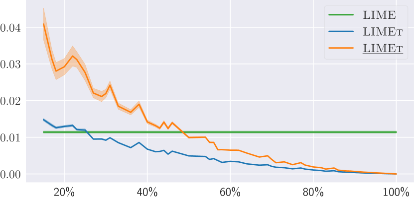
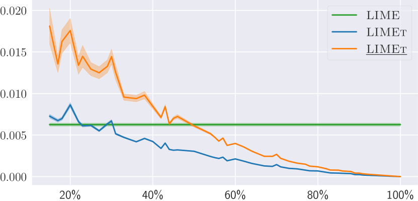
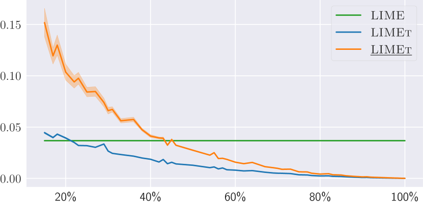
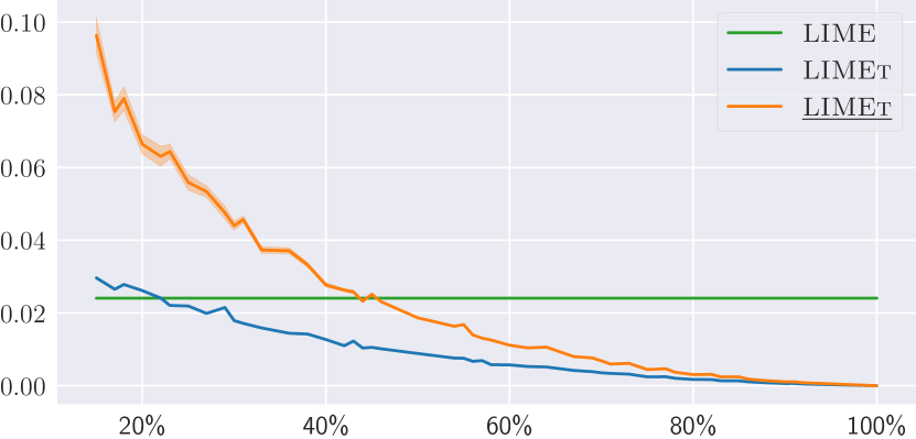
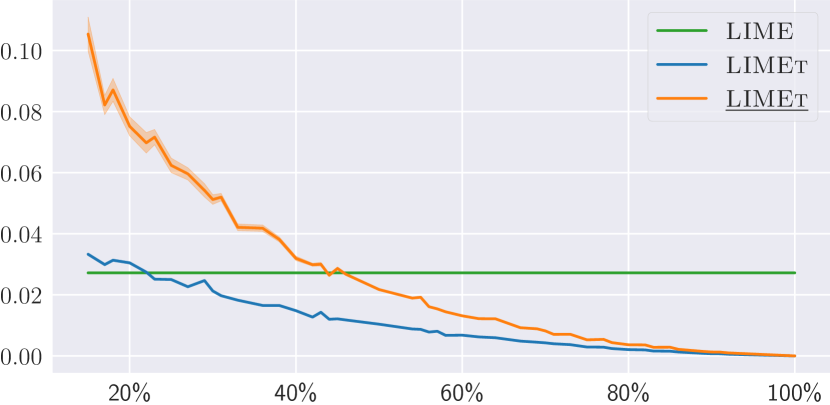
Tables 1 and 2 show that our base method – LIMEt – provides more faithful explanations than LIME. The variant of LIMEtree that boasts full fidelity for model-driven explanations – LIMEt – achieves performance somewhere between LIMEt and LIME. When compared to LIMEt, the fidelity drop suffered by LIMEt is due to sub-optimal predictions made by the tree leaves for the majority of the interpretable space since the surrogate is explicitly tuned to be faithful for the minimal interpretable data points. Surrogate trees without a depth bound – composed by LIMEt^† – achieve full fidelity across the board, which is expected since this variant of LIMEtree is expressive enough to model the entire interpretable data space, constructing one leaf for each instance if needed.

Complexity

Even though LIMEtree can offer explanations that are more truthful than those output by LIME, these may be generated by relatively convoluted trees. To better understand this phenomenon, we investigate the relation between the complexity of the surrogate trees and their fidelity. Since various images may have different number of super-pixels, i.e., interpretable features, our formulation of the depth-based tree complexity $\Omega$ given by Equation 4 accounts for that by scaling the tree depth in relation to the number of segments – this metric can be interpreted as tree completeness level. It allows us to study how building surrogate trees of higher complexity influences their fidelity, and how these properties compare to a baseline given by linear surrogates whose complexity is fixed. The results of our experiments are presented in Figure 7.

Regardless of the fidelity metric, number of explained classes and their evaluation setup, LIMEt relies on 20–30% and LIMEt needs at most 50% of all the interpretable features to perform on par with LIME. LIMEt requires deeper trees to achieve the same level of performance as LIMEt since the post-processing step applied to ensure full fidelity of model-driven explanations (Algorithm 2) causes the surrogate to be a sub-optimal predictor for most data points. By allowing deeper trees we reduce the impurity of their leaves, which improves the overall performance of the surrogates – an intuitive relation between the complexity of the trees and their fidelity. These empirical observations complement and support the discussion about explanation comprehensibility presented in Section 4.3.

5.3. User Study

To assess real-life usefulness of LIMEtree explanations, we ran a pilot user study comparing our approach with LIME, which is an established black-box surrogate explainer. To this end, we recruited eight participants with diverse skills and backgrounds, whom we served non-interactive insights based on surrogate multi-output trees. Specifically, the participants were shown the structure of the surrogate model similar to the visualisation displayed in Figure 2. The study subjects were also provided with a brief tutorial explaining how to manually parse the tree to obtain different kinds of explanations as well as a description of the meaning and purpose thereof.

The study consisted of two sections – one devoted to LIME and one concerning LIMEtree – displaying an image divided into three super-pixels, with each segment enclosing a unique object, e.g., a cat, a dog and a ball. The two most pertinent predictions for each object output by the underlying black-box model were explained with both methods and presented to the participants. For example, tabby and tiger cat for the cat object; golden retriever and Labrador retriever for the dog object; and tennis ball and croquet ball for the ball object. The explainee was exposed to six LIME explanations, each one showing the influence of the three segments (one per object), and a single multi-output tree of depth three modelling all six predictions simultaneously. The participants were asked about the expected behaviour of the black-box model in relation to any two out of the three displayed objects for each explainability method – six questions in total as the relations are assumed to be non-reflective. For example, “How does the presence of the cat object affect the model’s confidence of a presence of the dog object?”, with three possible answers: confidence decreases, confidence not affected and confidence increases.

This particular question formulation was chosen to avoid a bias towards either of the explainability methods since we could neither ask for the importance or influence of each object on a particular prediction (LIME’s domain), nor the relation between an object and a prediction, e.g., a counterfactual question (LIMEtree’s domain). Additionally, the participants were exposed to the explanations in a random order to mitigate one method affecting the perception of the other. We also did not disclose the name of the technique used to generate the explanations to avoid the familiarity of LIME influencing our results. Before viewing the explanations, the participants were asked to answer a similar set of questions using only their intuition. We used these responses to assess whether the explainees still relied on their intuition when explicitly asked to work with the explanations instead.

Our findings show that LIMEtree helped the participants to correctly answer 25% more of the questions in comparison to LIME. The negligible overlap between the responses based on the participants’ intuition and for either of the two explainability methods shows that the explainees relied on the provided insights when instructed to do so. Despite the majority of the participants having a machine learning background, and in a few cases some familiarity with XAI and IML concepts, all of our users found the process of manually extracting LIMEtree explanations challenging or daunting and rated the experience as either difficult or very difficult. This result is somewhat expected as these explanations are meant to be extracted algorithmically and presented via an interactive interface; nonetheless, despite this difficulty our method was still able to offer useful insights, showing great future potential. In contrast, all of the participants indicated that using LIME explanations was either easy or very easy, which in conjunction with poor user performance when compared to LIMEtree suggests that the explainees were overconfident in their judgement of the quality and usefulness of LIME explanations as well as prone to misinterpreting their meaning. We conclude that LIMEtree explanations are promising and when extracted algorithmically and delivered through an intuitive user interface (instead of leaving these tasks to the user) they can provide truthful and helpful insights that satisfy the needs of explainees.

6. Related Work

Multi-class explainability appears to be an under-explored area of research. The most prominent paper addressing this challenge expands Generalised Additive Models (GAMs (Hastie and Tibshirani, 1986)), which are inherently transparent and powerful predictors popular in high-stakes applications (Lou et al., 2012), to multiple classes (Zhang et al., 2019b). Surrogate explainability, one the other hand, has received considerable attention in the literature (Ribeiro et al., 2016; Sokol et al., 2019; Sokol, 2021; Sokol et al., 2022a; Sokol and Flach, 2020b). This suite of model-agnostic, post-hoc and often data-universal techniques can be used to explain:

• an individual prediction by building a local surrogate around the explained instance, e.g., LIME (Ribeiro et al., 2016), which uses a sparse linear regression;

• a collection of predictions by fitting a surrogate to a neighbourhood spanning a cohort of instances desired to be explained; or

• the inner workings of an entire black-box model by approximating its behaviour with a global surrogate, e.g., TREEPAN (Craven and Shavlik, 1996), which is based on a decision tree.

High modularity and flexibility of these explainers (Sokol et al., 2019) encouraged the research community to compose their different variant, some of which use decision trees as the (local) surrogate model (Waa et al., 2018; Shi et al., 2019; Sokol et al., 2019; Sokol, 2021). Waa et al. (2018) showed how a local one-vs-rest classification tree can be used to produce contrastive explanations; and Shi et al. (2019) fitted a local shallow regression tree and used its structure as an explanation. Both of these methods use a local tree surrogate, however none of them utilises the full explainability (and interactivity) potential that they enable. Explainability of decision trees (Sokol and Flach, 2018; Sokol, 2021) and their ensembles (Tolomei et al., 2017) have also been investigated outside of the surrogate deployment context. Sokol and Flach (2018, 2020c) showed how to extract personalised counterfactual explanations by interacting with a decision tree via a voice interface and Tolomei et al. (2017) introduced a method to explain predictions made by ensembles of decision tree classifiers with class-contrastive counterfactuals.

Research on personalised and interactive explainability has also been largely neglected up until recently. While the pivot in XAI and IML towards human-centred explainability (Miller, 2018; Miller et al., 2017) was premised on people’s preference for contrastive and social (dynamic, dialogue-like and bi-directional) explanations, since they occur naturally in human interactions, the former aspect received considerably more attention than the latter. Schneider and Handali (2019) have recently reviewed an array of explainability approaches accounting for their interactivity – which allows the explainees to guide the explainer, hence receive tailored explanations – leading them to conclude that personalised explanations are generally unavailable. While this is true for practical explainability approaches, extensive research has been undertaken to analyse theoretical properties and various frameworks to model explanatory interactions between two intelligent agents, be them humans, machines or one of each (Walton, 2007; Arioua and Croitoru, 2015; Madumal et al., 2019). An alternative line of work considered integrating multiple explanation modalities and hypothesised how interactions with such systems, as opposed to individual explanations, could look like in the real life (Weld and Bansal, 2019). On the algorithmic plane, otherwise static explainability approaches, such as partial dependence plots (Friedman, 2001), were fitted into interactive user interfaces (Krause et al., 2016b, a) to provide the explainee with a freedom to explore these insights; and a mixture of explainability and interactivity was used to refine, e.g., personalise, improve or debug, data modelling techniques such as clustering (Kim et al., 2015) and naïve Bayes classification (Kulesza et al., 2015).

7. Conclusions and Future Work

In this paper we introduced the novel concept of multi-class explainability and proposed a local surrogate explainer of black-box predictions based on multi-output regression trees – called LIMEtree – that addresses this challenge. We analysed various properties and guarantees of our technique and reported requirements necessary for it to achieve full fidelity, which makes it an attractive explainability tool. This discussion led to practical design recommendations and operationalisation guidelines outlining how these concepts can be realised in practice. We then demonstrated how LIMEtree improves upon LIME (Ribeiro et al., 2016) – in terms of both explanation quality and informativeness – by simultaneously modelling multiple classes, and discussed numerous benefits – with respect to the diversity of explanation types and their propensity for interactive personalisation – of using trees as the surrogate model. We supported these claims with an array of explanation examples produced by our method, an assessment of its properties based on XAI and IML desiderata as well as a collection of quantitative experiments and a preliminary user study.

At present, some explanation types showcased in this paper have to be manually extracted from the (surrogate) tree, which we will address in future work with appropriate algorithmic tools. Specifically, we will look into parsing the tree structure to generate ante-hoc counterfactual explanations that account for user-specified heuristics. We will further work on interactive explainability by supplementing LIMEtree with an interface via which the explainees could request, explore and personalise the explanations. Having implemented user-facing components, we will carry out user studies to empirically evaluate the influence of each explanation type on the perceived improvement in transparency and assess the benefits of the interactive explanatory process over static explanations. More generally, we will investigate other techniques capable of realising the multi-class explainability paradigm.